Horizons as boundary conditions in spherical symmetry

Abstract

We initiate the development of a horizon-based initial (or rather final) value formalism to describe the geometry and physics of the near-horizon spacetime: data specified on the horizon and a future ingoing null boundary determine the near-horizon geometry. In this initial paper we restrict our attention to spherically symmetric spacetimes made dynamic by matter fields. We illustrate the formalism by considering a black hole interacting with a) inward-falling, null matter (with no outward flux) and b) a massless scalar field. The inward-falling case can be exactly solved from horizon data. For the more involved case of the scalar field we analytically investigate the near slowly evolving horizon regime and propose a numerical integration for the general case.

I Introduction

This paper begins an investigation into what horizon dynamics can tell us about external black hole physics. At first thought this might seem obvious: if one watches a numerical simulation of a black hole merger and sees a post-merger horizon ringdown (see for example https://www.black holes.org (2018)) then it is natural to think of that oscillation as a source of emitted gravitational waves. However this cannot be the case. Neither event nor apparent horizons can actually send signals to infinity: apparent horizons lie inside event horizons which in turn are the boundary for signals that can reach infinityHawking and Ellis (2011). It is not horizons themselves that interact but rather the “near horizon” fields. This idea was (partially) formalized as a “stretched horizon” in the membrane paradigmThorne et al. (1986).

Then the best that we can hope for from horizons is that they act as a proxy for the near horizon fields with horizon evolution reflecting some aspects of their dynamics. As explored in Jaramillo et al. (2012a, b, 2011); Rezzolla et al. (2010); Gupta et al. (2018) there should then be a correlation between horizon evolution and external, observable, black hole physics.

Robinson-Trautman spacetimes (see for example Griffiths and Podolsky (2009)) demonstrate that this correlation cannot be perfect. In those spacetimes there can be outgoing gravitational (or other) radiation arbitrarily close to an isolated (equilibrium) horizonAshtekar et al. (2000a). Hence our goal is two-fold: both to understand the conditions under which a correlation will exist and to learn precisely what information it contains.

The idea that horizons should encode physical information about black hole physics is not new. The classical definition of a black hole as the complement of the causal past of future null infinity Hawking and Ellis (2011) is essentially global and so defines a black hole spacetime rather than a black hole in some spacetime. However there are also a range of geometrically defined black hole boundaries based on outer and/or marginally trapped surfaces that seek to localize black holes. These include apparentHawking and Ellis (2011), trappingHayward (1994a), isolated Ashtekar et al. (1999, 2000b, 2000a); Hayward (1994b) and dynamical Ashtekar and Krishnan (2003) horizons as well as future holographic screens Bousso and Engelhardt (2015). These quasilocal definitions of black holes have successfully localized black hole mechanics to the horizonAshtekar et al. (1999, 2000b); Ashtekar and Krishnan (2003); Booth and Fairhurst (2004); Bousso and Engelhardt (2015); Hayward (1994a) and been particularly useful in formalizing what it means for a (localized) black hole to evolve or be in equilibrium. They are used in numerical relativity not only as excision surfaces (see, for example the discussions in Baumgarte and Shapiro (2010); Thornburg (2007)) but also in interpreting physics (for example Dreyer et al. (2003); Cook and Whiting (2007); Chu et al. (2011); Jaramillo et al. (2012a, b, 2011); Rezzolla et al. (2010); Lovelace et al. (2015); Gupta et al. (2018); Owen et al. (2017)).

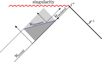
(a) Future and past domains of dependence for ${\cal H}_{\text{dynamic}}$: standard (3+1) IVP

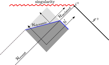
(b) Future and past domains of dependence for ${\cal H}_{\text{dynamic}}\cup{\cal N}$: characteristic IVP

Figure 1: Domains of dependence of initial data

In this paper we work to quantitatively link horizon dynamics to observable black hole physics. To establish an initial framework and build intuition we for now restrict our attention to spherically symmetric marginally outer trapped tubes (MOTTs) in similarly symmetric spacetimes. Matter fields are included to drive the dynamics. Our primary approach is to take horizon data as a (partial) final boundary condition that is used to determine the fields in a region of spacetime in its causal past. In particular these boundary conditions constrain the geometry and physics of the associated “near horizon” spacetime. The main application that we have in mind is interpreting the physics of evolving horizons that have been generated by either numerical simulations or theoretical considerations.

Normally, data on a MOTT by itself is not sufficient to specify any region of the external spacetime. As shown in FIG. 1(a) even for a spacelike MOTT (a dynamical horizon) the region determined by a standard (3+1) initial value formulation would lie entirely within the event horizon. More information is needed to determine the near-horizon spacetime and hence in this paper we work with a characteristic initial value formulation Rendall (1990); Sachs (1962); Winicour (2012, 2013); Mädler and Winicour (2016) where extra data is specified on a null surface $\mathcal{N}$ that is transverse to the horizon (FIG. 1(b)). Intuitively the horizon records inward-moving information while $\mathcal{N}$ records the outward-moving information. Together they are sufficient to reconstruct the spacetime.

There is an existing literature that studies spacetime near horizons, however it does not exactly address this problem. Most works focus on isolated horizons. Li and Lucietti (2016) and Li and Lucietti (2018) examine spacetime near an isolated extremal horizon as a Taylor series expansion of the horizon while Krishnan (2012) and Lewandowski and Li (2018) study spacetime near more general isolated horizons but in a characteristic initial value formulation with the extra information specified on a transverse null surface. Booth (2013) studied both the isolated and dynamical case though again as a Taylor series expansion off the horizon. In the case of the Taylor expansions, as one goes to higher and higher orders one needs to know higher and higher order derivatives of metric quantities at the horizon to continue the expansion. While the current paper instead investigates the problem as a final value problem, it otherwise closely follows the notation of and uses many results from Booth (2013).

It is organized as follows. We introduce the final value formulation of spherically symmetric general relativity in Sec.II. We illustrate this for infalling null matter in III and then the much more interesting massless scalar field in Sec.IV. We conclude with a discussion of results in Sec.V.

II Formulation

II.1 Coordinates and metric

We work in a spherically symmetric spacetime (${\cal M},g$) and a coordinate system whose non-angular coordinates are $\rho$ (an ingoing affine parameter) and $v$ (which labels the ingoing null hypersurfaces and increases into the future). Hence, $g_{\rho\rho}=0$ and the curves tangent to the future-oriented inward-pointing

$$N=\frac{\partial}{\partial\rho}$$ (1)

are null. We then scale $v$ so that $\mathcal{V}=\frac{\partial}{\partial v}$ satisfies

$$\mathcal{V}\cdot N=-1.$$ (2)

One coordinate freedom still remains: the scaling of the affine parameter on the individual null geodesics

$$\tilde{\rho}=f(v)\rho\,.$$ (3)

In subsection II.3 we will fix this freedom by specifying how $N$ is to be scaled along the $\rho=0$ surface $\Sigma$ (which we take to be a black hole horizon).

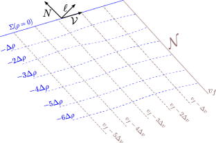
Figure 2: Coordinate system for characteristic evolution. We work with final boundary conditions so that in the region of interest $\rho<0$.

Next we define the future-oriented outward-pointing null normal to the spherical surfaces $S_{(v,\rho)}$ as $\ell^{a}$ and scale so that

$$\ell\cdot N=-1\,.$$ (4)

With this choice the four-metric $g_{ab}$ and induced two-metric $\tilde{q}_{ab}$ on the $S_{(v,\rho)}$ are related by

$$g^{ab}=\tilde{q}^{ab}-\ell^{a}N^{b}-N^{a}\ell^{b}\,.$$ (5)

Further for some function $C$ we can write

$${\cal V}=\ell-CN\,.$$ (6)

The coordinates and normal vectors are depicted in FIG.2 and give the following form of the metric:

$$ds^{2}=2C(v,\rho)\text{d}v^{2}-2\text{d}v\,\text{d}\rho+R(v,\rho)^{2}\text{d}\Omega^{2}$$ (7)

where $R(v,\rho)$ is the areal radius of the $S_{(v,\rho)}$ surfaces. Note the similarity to ingoing Eddington-Finkelstein coordinates for a Schwarzschild black hole. However $\nicefrac{{\partial}}{{\partial\rho}}$ points inwards as opposed to the outward oriented $\nicefrac{{\partial}}{{\partial r}}$ in those coordinates (hence the negative sign on the $\mbox{d}v\mbox{d}\rho$ cross-term).

Typically, as shown in FIG.2 we will be interested in regions of spacetime that are bordered in the future by a surface $\Sigma$ of indeterminate sign on which $\rho=0$ and a null $\mathcal{N}$ which is one of the $v$=constant surfaces (and so $\rho<0$ in the region of interest). We will explore how data on those surfaces determines the region of spacetime in their causal past.

II.2 Equations of motion

In this section we break up the Einstein equations relative to these coordinates, beginning by defining some geometric quantities that appear in the equations.

First the null expansions for the $\ell^{a}$ and $N^{a}$ congruences are

$$\theta_{(\ell)} =\tilde{q}^{ab}\nabla_{a}\ell_{b}=\frac{2}{R}{\cal L}\,_{\ell}R\quad\mbox{and}$$ (8)

$$\theta_{(N)} =\tilde{q}^{ab}\nabla_{a}N_{b}=\frac{2}{R}{\cal L}\,_{N}R=\frac{2}{R}R_{,\rho}.$$ (9)

while the inaffinities of the null vector fields are

$$\kappa_{N} =-N^{a}N_{b}\nabla_{a}\ell^{b}=0\quad\mbox{and}$$ (10)

$$\kappa_{\mathcal{V}} =\kappa_{\ell}-C\kappa_{N}=-\ell^{a}N_{b}\nabla_{a}\ell^{b}\,.$$ (11)

By construction $\kappa_{N}=0$ and so we can drop it from our equations and henceforth write

$$\kappa\equiv\kappa_{\mathcal{V}}=\kappa_{\ell}\,.$$ (12)

Finally the Gaussian curvature of $S_{(v,\rho)}$ is:

$$\tilde{K}=\frac{1}{R^{2}}\,.$$ (13)

Then these curvature quantities are related by constraint equations along the surfaces of constant $\rho$

$$\mathcal{L}_{\mathcal{V}}R= {\cal L}\,_{\ell}R-C{\cal L}\,_{N}R\quad\text{(by definition)}\,,$$ (14)

$$\mathcal{L}_{\mathcal{V}}\theta_{(\ell)}= \kappa\,\theta_{(\ell)}+C\left(\frac{1}{R^{2}}+\theta_{(N)}\theta_{(\ell)}-G_{\ell N}\right)$$

$$-\left(G_{\ell\ell}+\frac{1}{2}\theta_{(\ell)}^{2}\right)\,,$$ (15)

$$\mathcal{L}_{\mathcal{V}}\theta_{(N)}= -\kappa\,\theta_{(N)}-\left(\frac{1}{R^{2}}+\theta_{(N)}\theta_{(\ell)}-G_{\ell N}\right)$$

$$+C\left(G_{\!N\!N}+\frac{1}{2}\theta_{(N)}^{2}\right),$$ (16)

and “time” derivatives in the $\rho$ direction

$${\cal{L}}_{N}\theta_{(N)}= -\frac{\theta_{(N)}^{2}}{2}-G_{\!N\!N},$$ (17)

$${\cal{L}}_{N}\theta_{(\ell)}= -\frac{1}{R^{2}}-\theta_{(N)}\theta_{(\ell)}+G_{\ell N},$$ (18)

$${\cal{L}}_{N}\kappa= \frac{1}{R^{2}}+\frac{1}{2}\theta_{(N)}\theta_{(\ell)}-\frac{1}{2}G_{\tilde{q}}-G_{\ell N},$$ (19)

where by the choice of the coordinates

$$\kappa={\cal{L}}_{N}C\,.\\$$ (20)

These equations can be derived from the variations for the corresponding geometric quantities (see, for example, Booth and Fairhurst (2007) and Booth (2013)) and of course are coupled to the matter content of the system through the Einstein equations

$$G_{ab}=8\pi T_{ab}\;.$$ (21)

Using (8) and (9) we can rewrite the constraint and evolution equations in terms of the metric coefficients and coordinates as:

$$R_{,v}= \,R_{\ell}-CR_{N}\,,\quad$$ (22)

$$R_{\ell,v}= \,\kappa R_{\ell}+\frac{C\left(1+4R_{\ell}R_{N}\right)}{2R}-\frac{R}{2}\,(G_{\ell\ell}+CG_{\ell N})\,,$$ (23)

$$R_{N,v}= -\kappa R_{N}-\frac{\left(1+4R_{\ell}R_{N}\right)}{2R}+\frac{R}{2}\,(G_{\ell N}+CG_{N\!N}).$$ (24)

and

$$R_{,\rho\rho} =-\frac{R}{2}\,G_{\!N\!N},$$ (25)

$$({RR_{\ell}})_{,\rho} =-\frac{1}{2}+\frac{R^{2}}{2}G_{\ell N},$$ (26)

$$C_{,\rho\rho} =\frac{1}{R^{2}}+\frac{2R_{\ell}R_{N}}{R^{2}}-\frac{1}{2}G_{\tilde{q}}-G_{\ell N},$$ (27)

where

$$\kappa=C_{,\rho}.\\$$ (28)

For those who don’t want to work through the derivations of Booth and Fairhurst (2007) and Booth (2013), these can also be derived fairly easily (thanks to the spherical symmetry) from an explicit calculation of the Einstein tensor for (7).

II.3 Final Data

We will focus on the case where $\rho=0$ is an isolated or dynamical horizon $H$. Thus

$$\theta_{(\ell)}\overset{\scriptscriptstyle{H}}{=}0\quad\Longleftrightarrow\quad R_{\ell}\overset{\scriptscriptstyle{H}}{=}0\;.$$ (29)

The notation $\overset{\scriptscriptstyle{H}}{=}$ indicates that the equality holds on $H$ (but not necessarily anywhere else). Further we can use the coordinate freedom (3) to set

$$R_{N}\overset{\scriptscriptstyle{H}}{=}R_{,\rho}|\overset{\scriptscriptstyle{H}}{=}-1\,.$$ (30)

On $H$, the constraints (22)-(24) fix three of

$$\{C,\kappa,R,R_{\ell},R_{N},G_{\ell\ell},G_{\ell N},G_{NN}\}$$ (31)

given the other five quantities. For example if $R_{\ell}\overset{\scriptscriptstyle{H}}{=}0$ and $R_{N}\overset{\scriptscriptstyle{H}}{=}-1$ then (22) and (23) give

$$R_{,v}\overset{\scriptscriptstyle{H}}{=}C\overset{\scriptscriptstyle{H}}{=}\frac{R^{2}G_{\ell\ell}}{1-R^{2}G_{\ell N}}$$ (32)

and (24) gives

$$\kappa=C_{\rho}\overset{\scriptscriptstyle{H}}{=}\frac{1}{2R}-\frac{R}{2}\left(G_{\ell N}+CG_{\!N\!N}\right)\,.$$ (33)

Thus if $G_{\ell\ell}$ and $G_{\ell N}$ are specified for $v_{i}\leq v\leq v_{f}$ on $H$ and $R(v_{f})\overset{\scriptscriptstyle{H}}{=}R_{f}$ then one can solve (32) to find $R$ over the entire range. Equivalently one could take $R$ and one of $G_{\ell\ell}$ or $G_{\ell N}$ as primary and then solve for the other component of the stress-energy.

Of course, in general the matter terms will also be constrained by their own equations; these will be treated in later sections. Further data on $\rho=0$ will generally not be sufficient to fully determine the regions of interest and data will also be needed on an $\mathcal{N}$. Again this will depend on the specific matter model.

Nevertheless if there is a MOTT at $\rho=0$ then the constraints provide significant information about the horizon. If $G_{\ell\ell}=0$ (no flux of matter through the horizon) then we have an isolated horizon with $C=0$, a constant $R$ and a null $H$. This is independent of other components of the stress-energy.

Alternatively if $G_{\ell\ell}>0$ (the energy conditions forbid it to be negative) and $G_{\ell N}<1/R^{2}$ then we have a dynamical horizon with $C>0$, increasing $R$ and spacelike $H$. Note that this growth doesn’t depend in any way on $G_{\!N\!N}$: there is no sense in which the growing horizon “catches” outward moving matter and hence grows even faster. The behaviour of the coordinates relative to isolated and dynamical horizons along with $\mathscr{I}^{+}$ is illustrated in FIG.3.

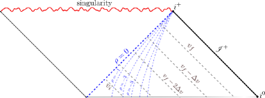
(a) Isolated horizon : $d\rho$ is timelike for all values of $\rho$

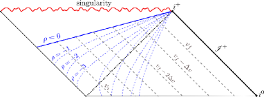
(b) Dynamical horizon : $d\rho$ is spacelike for small values of $\rho$ and eventually becomes timelike for large values of $\rho$

Figure 3: Spacetime foliation for isolated and dynamical horizons

The evolution equations are more complicated and depend on the matter field equations. We examine two such cases in the following sections.

III Traceless inward flowing null matter

As our first example consider matter that falls entirely in the inward $N$-direction with no outward $\ell$-flux. Then data on the horizon should be sufficient to entirely determine the region of spacetime traced by the horizon-crossing inward null geodesics: there are no dynamics that don’t involve the horizon.

Translating these words into equations, we assume that

$$T_{ab}N^{a}N^{b}=0$$ (34)

(no matter flows in the outward $\ell$-direction). Further, for simplicity we also assume that it is trace-free

$$g^{ab}T_{ab}=0\quad\Leftrightarrow\quad T_{\tilde{q}}=2T_{\ell N}\;.$$ (35)

Then we can solve for the metric using only the Bianchi identities

$$\nabla_{a}G^{ab}=0,$$ (36)

without any reference to detailed equations of motion for the matter field. Keeping spherical symmetry but temporarily suspending the other simplifying assumptions they may be written as:

$$\mathcal{L}_{\ell}(R^{2}G_{\!N\!N})+ \mathcal{L}_{N}(R^{2}G_{\ell N})+R^{2}(2\kappa_{\ell}G_{\!N\!N})$$

$$+\frac{1}{2}R^{2}\theta_{(N)}G_{\tilde{q}}=0,$$ (37)

$$\mathcal{L}_{N}(R^{2}G_{\ell\ell})+ \mathcal{L}_{\ell}(R^{2}G_{\ell N})+R^{2}(-2\kappa_{N}G_{\ell\ell})$$

$$+\frac{1}{2}R^{2}\theta_{(\ell)}G_{\tilde{q}}=0\,.$$ (38)

In terms of metric coefficients with $\kappa_{N}=0$ plus (34) and (35) these reduce to:

$$(R^{4}G_{\ell N})_{,\rho}=0\,\,\text{ and }$$ (39)

$$(R^{2}G_{\ell\ell})_{,\rho}+\frac{1}{R^{2}}(R^{4}G_{\ell N})_{,v}=0.$$ (40)

As we shall see, this class of matter includes interesting examples like Vaidya-Reissner-Nordström (charged null dust).

We now demonstrate that given knowledge of $G_{\ell\ell}$ and $G_{\ell N}$ over a region of horizon $\bar{H}=\{H:v_{i}\leq v\leq v_{f}\}$ as well as $R(v_{f})\overset{\scriptscriptstyle{H}}{=}R_{f}$ we can determine the spacetime everywhere out along the horizon-crossing inward null geodesics.

III.1 On the horizon

First consider the constraints on $\bar{H}$. In this case it is tidier to take $R$ and $G_{\ell N}$ as primary. Then we can specify

$$R\overset{\scriptscriptstyle{H}}{=}R_{H}(v)\quad\mbox{and}\quad G_{\ell N}\overset{\scriptscriptstyle{H}}{=}\frac{Q(v)}{R_{H}^{4}}$$ (41)

for some functions $R_{H}(v)$ (dimensions of length) and $Q_{H}(v)$ (dimensions of length squared) where the form of the latter is chosen for future convenience. Then

$$C\overset{\scriptscriptstyle{H}}{=}R_{H,v}$$ (42)

and by (32)

$$G_{\ell\ell}\overset{\scriptscriptstyle{H}}{=}R_{H,v}\left(\frac{1}{R_{H}^{2}}-\frac{Q}{R_{H}^{4}}\right)$$ (43)

Finally by (33),

$$\kappa\overset{\scriptscriptstyle{H}}{=}C_{\rho}\overset{\scriptscriptstyle{H}}{=}\frac{1}{2R_{H}}\left(1-\frac{Q}{R_{H}^{2}}\right)\,.$$ (44)

III.2 Off the horizon

Next, integrate away from $\bar{H}$. First with $G_{\!N\!N}=0$ (25) can be integrated with initial condition (30) to give

$$R(v,\rho)=R_{H}(v)-\rho\,.$$ (45)

Then with (41) we can integrate (39) to find

$$G_{\ell N} =\frac{Q}{R^{4}}$$ (46)

and use this result and (43) to integrate(40) to get

$$G_{\ell\ell} =\frac{\left(R_{H}^{2}-Q\right)R_{H,v}}{R_{H}^{2}R^{2}}+\frac{\rho\,Q_{,v}}{R_{H}R^{3}}\,.$$ (47)

With these results in hand and initial condition $R_{\ell}\overset{\scriptscriptstyle{H}}{=}0$ we integrate (26) to get

$$R_{\ell}=\frac{\rho(Q-R_{H}^{2}+\rho R_{H})}{2R^{2}R_{H}}$$ (48)

and finally with initial conditions (32) and (33) we can integrate (27) to find

$$C=R_{H,v}-R_{\ell}\,.$$ (49)

III.3 Comparison with Vaidya-Reissner-Nordström

We can now compare this derivation to a known example. The Vaidya-Reissner-Nordström (VRN) metric takes the form

$$\mbox{d}s^{2}=-\left(1-\frac{2m(v)}{r}+\frac{q(v)^{2}}{r^{2}}\right)\mbox{d}v^{2}+2\mbox{d}v\mbox{d}r+r^{2}\mbox{d}\Omega^{2}$$ (50)

where the apparent horizon $r_{H}=m+\sqrt{m^{2}-q^{2}}$ and $r$ is an affine parameter of the ingoing null geodesics. To put it into the form of (7) where the affine parameter measures distance off the horizon we make the transformation

$$r=r_{H}-\rho$$ (51)

whence the metric takes the form

$$\mbox{d}s^{2}= -\left(2r_{H,v}-\frac{\rho\left(q^{2}-r_{H}(r_{H}-\rho)\right)}{r_{H}(r_{H}-\rho)^{2}}\right)\mbox{d}v^{2}$$ (52)

$$-2\mbox{d}v\mbox{d}\rho+(r_{H}-\rho)^{2}\mbox{d}\Omega^{2}\,.$$

That is

$$C =r_{H,v}-\frac{\rho\left(q^{2}-r_{H}(r_{H}-\rho)\right)}{2r_{H}(r_{H}-\rho)^{2}}$$ (53)

$$R =r_{H}-\rho$$ (54)

and on the horizon

$$C\overset{\scriptscriptstyle{H}}{=}r_{H,v}\qquad\mbox{and}\qquad R\overset{\scriptscriptstyle{H}}{=}r_{H}$$ (55)

as expected.

To do a complete match we calculate the rest of the quantities. First appropriate null vectors are

$$\ell =\frac{\partial}{\partial v}+\left(r_{H,v}-\frac{\rho\left(q^{2}-r_{H}(r_{H}-\rho)\right)}{2r_{H}(r_{H}-\rho)^{2}}\right)\frac{\partial}{\partial\rho}$$ (56)

$$N =\frac{\partial}{\partial\rho}\,.$$ (57)

Then direct calculation shows that

$$R_{\ell} =-\frac{\rho\left(q^{2}-r_{H}(r_{H}-\rho)\right)}{2r_{H}(r_{H}-\rho)^{2}}$$ (58)

$$R_{N} =-1$$ (59)

and

$$G_{\ell\ell} =\frac{\left(r_{H}^{2}-q^{2}\right)r_{H,v}}{r_{H}^{2}r^{2}}+\frac{2\rho qq_{,v}}{r_{H}r^{3}}$$ (60)

$$G_{\ell N} =\frac{q^{2}}{(r_{H}-\rho)^{2}}$$ (61)

$$G_{NN} =0$$ (62)

$$G_{q} =\frac{2q^{2}}{(r_{H}-\rho)^{2}}\;.$$ (63)

It is clear that with $R_{H}=r_{H}$ and $Q=q^{2}$ our general results (41)-(49) give rise to the VRN spacetime (as they should).

As expected the data on the horizon is sufficient to determine the spacetime everywhere back out along the ingoing null geodesics: we simply solve a set of (coupled) ordinary differential equations along each curve. With the matter providing the only dynamics and that matter only moving inwards along the geodesics the problem is quite straightforward. In this case there is no need to specify extra data on $\mathcal{N}$.

We now turn to the more interesting case where the dynamics are driven by a scalar field for which there will be both inward and outward fluxes of matter.

IV Massless scalar field

Spherical spacetimes containing a massless scalar field $\phi(v,\rho)$ are governed by the stress energy tensor given by,

$$T_{ab} =\nabla_{a}\phi\nabla_{b}\phi-\frac{1}{2}g_{ab}\nabla^{c}\phi\nabla_{c}\phi$$ (64)

This system has nonvanishing inward and outward fluxes which are,

$$T_{\ell\ell} =(\phi_{\ell})^{2}$$ (65)

$$T_{NN} =(\phi_{N})^{2}.$$ (66)

Here and in the following keep in mind that $N=\frac{\partial}{\partial\rho}$ and so $\phi_{N}=\phi_{,\rho}$. We also observe from (64) that,

$$T_{\ell N}=0.$$ (67)

These fluxes are related by the wave equation

$$\Box_{g}\phi:=\nabla^{\alpha}\nabla_{\alpha}\phi=0\implies{\left(R\phi_{\ell}\right)_{,\rho}=-R_{\ell}\phi_{,\rho}}.$$ (68)

For our purposes we are not particularly interested in the value of $\phi$ itself but rather in the associated net flux of energies in the ingoing and outgoing null direction. Hence we define

$$\Phi_{\ell}=\sqrt{4\pi}R\phi_{\ell}\quad\mbox{and}\quad\Phi_{N}=\sqrt{4\pi}R\phi_{N}\,.$$ (69)

Respectively these are the square roots of the scalar field energy fluxes in the $N$ and $\ell$ directions. That is, over a sphere of radius $R$, $\Phi_{\ell}$ is the square root of the total integrated flux in the $N$-direction and $\Phi_{N}$ is the square root of the total integrated flux in the $\ell$-direction. Though not strictly correct, we will often refer to $\Phi_{\ell}$ and $\Phi_{N}$ themselves as fluxes.

Then (68) becomes

$$\Phi_{\ell,\rho}=-\frac{R_{\ell}\Phi_{N}}{R}\,$$ (70)

or, making use of the fact that $\phi_{,v\rho}=\phi_{,\rho v}$,

$$\Phi_{N,v}=-\kappa\Phi_{N}-C\Phi_{N,\rho}-\frac{R_{N}\Phi_{\ell}}{R}\,.$$ (71)

These can usefully be understood as advection equations with sources. Recall that a general homogeneous advection equation can be written in the form

$$\frac{\partial\psi}{\partial t}+C\frac{\partial\psi}{\partial x}=0$$ (72)

where $C$ is the speed of flow of $\psi$: if $C$ is constant then this has the exact solution

$$\psi=\psi(x-Ct)$$ (73)

and so any pulse moves with speed $\frac{dx}{dt}=C$. Any non-homogeneous term corresponds to a source which adds or removes energy from the system. Then (70) tells us that the flux in the $N$-direction ($\Phi_{\ell})$ is naturally undiminished as it flows along a (null) surface of constant $v$ and increasing $\rho$. However the interaction with the flux in the $\ell$ direction can cause it to increase or decrease. Similarly (71) describes the flow of the flux in the $\ell$-direction ($\Phi_{N}$) along a surface of constant $\rho$ and increasing $v$. Rewriting with respect to the affine derivative (see Appendix B) $D_{v}=\partial_{v}+\kappa$ it becomes

$$D_{v}\Phi_{N}+C\Phi_{N,\rho}=-\frac{R_{N}\Phi_{\ell}}{R}\,.$$ (74)

Then, as might be expected, $\Phi_{N}$ naturally flows with coordinate speed $C$ (recall that $\ell=\frac{\partial}{\partial v}+C\frac{\partial}{\partial\rho}$ so this is the speed of outgoing light relative to the coordinate system) but its strength can be augmented or diminished by interactions with the outward flux.

IV.1 System of first order PDEs

Together (70) and (71) constitute a first-order system of partial differential equations for the scalar field. We now restructure the gravitational field equations in the same way.

First with respect to $\Phi_{\ell}$ and $\Phi_{N}$ the constraint equations (14)-(16) on constant $\rho$ surfaces become:

$$R_{,v} =R_{\ell}-CR_{N}$$ (75)

$$R_{\ell,v} =\kappa R_{\ell}+\frac{C\left(1+2R_{\ell}R_{N}\right)}{2R}-\frac{\Phi_{\ell}^{2}}{R}$$ (76)

$$R_{N,v} =-\kappa R_{N}-\frac{\left(1+2R_{\ell}R_{N}\right)}{2R}+\frac{C\Phi_{N}^{2}}{R}$$ (77)

while the “time”-evolution equations (17)-(19) are:

$${R_{,\rho\rho}=-\frac{\Phi_{N}^{2}}{R}}$$ (78)

$${\left(RR_{\ell}\right)_{,\rho}=-\frac{1}{2}}$$ (79)

$${C_{,\rho\rho}}\,\,{=\frac{1+2R_{\ell}R_{N}}{R^{2}}-\frac{2\Phi_{\ell}\Phi_{N}}{R^{2}}}\,.$$ (80)

Two of these equations can be simplified. First, integrating (79) from $\rho=0$ on which $R_{\ell}\overset{\scriptscriptstyle{H}}{=}0$ we find

$$R_{\ell}=-\frac{\rho}{2R}\,.$$ (81)

This can be substituted into (76) to turn it into an algebraic constraint

$$C=2\Phi_{\ell}^{2}-2R_{\ell}\left(\kappa R+R_{\ell}\right)\,.$$ (82)

Despite these simplifications, the presence of interacting outward and inward matter fluxes means that in contrast to the dust examples, this is truly a set of coupled partial differential equations. Hence we can expect that the matter and spacetime dynamics will be governed by off-horizon data in addition to data at $\rho=0$.

We reformulate as a system of first order PDEs in the following way. First designate

$$\;\;\{R,R_{N},\kappa,\Phi_{\ell},\Phi_{N}\}$$ (83)

as the primary variables. The secondary variables $\{R_{\ell},C\}$ are defined by (81) and (82) in terms of the primaries.

Next on $\rho=\mbox{constant}$ surfaces the primary variables are constrained by

$$R_{,v} =R_{\ell}-CR_{N}\;\;\mbox{and}$$ (84)

$$R_{N,v} =-\kappa R_{N}-\frac{1}{2R}\left(1+2R_{\ell}R_{N}-2C\Phi_{N}^{2}\right)$$ (85)

along with scalar flux equation (71) while their time evolution is governed by

$$R_{,\rho} =R_{N}$$ (86)

$$R_{N,\rho} =-\frac{\Phi_{N}^{2}}{R}$$ (87)

$$\kappa_{,\rho} =\frac{1}{R^{2}}\left(1+2R_{\ell}R_{N}-2\Phi_{\ell}\Phi_{N}\right)$$ (88)

$${\Phi}_{\ell,\rho} =-\frac{R_{\ell}\Phi_{N}}{R}\,.\,$$ (89)

We now consider how all of these equations may be used to integrate final data. The scheme is closely related to that used in Winicour (2012).

IV.2 Final data on $\bar{H}$ and $\bar{\mathcal{N}}$

In line with the depiction in FIG.1(b), we specify final data on $H\cup{\cal N}$ or rather on the sections $\bar{H}\cup\bar{{\cal N}}$ where

$$\bar{H} =\{(0,v)\in H:v_{i}\leq v\leq v_{f}\}\;\;\mbox{and}$$ (90)

$$\bar{\mathcal{N}} =\{(\rho,v_{f})\in\mathcal{N}:\rho_{i}\leq\rho\leq 0\}\,.$$

Their intersection sphere is $\bar{H}\cap\bar{{\cal N}}=(0,v_{f})$. Here and in what follows we suppress the angular coordinates.

The final data is

$$\bar{H}: \;\;\Phi_{\ell}$$ (91)

$$\bar{{\cal N}}: \;\;\Phi_{N}\;\;\mbox{and}$$

$$\bar{H}\cap\bar{\cal N}: \;\;R=R_{o}\;.$$

$\Phi_{\ell}$ on $\bar{H}$ is a function of $v$ while $\Phi_{N}$ on $\mathcal{\bar{N}}$ is a function of $\rho$. $R_{o}$ is a single number.

Further on ${H}$ we have

$$R_{\ell}\overset{\scriptscriptstyle{H}}{=}0\;\;\mbox{and}\;\;R_{N}\overset{\scriptscriptstyle{H}}{=}-1$$ (92)

where the null vectors are scaled in the usual way and, as before, the notation $\overset{\scriptscriptstyle{H}}{=}$ indicates that all quantities on both sides of the equality are evaluated on $H$.

This data can be used to evaluate $C$ and $R$ on $\bar{H}$. From (82) and (84)

$$C\overset{\scriptscriptstyle{H}}{=} \,2\Phi_{\ell}^{2}\;\;\mbox{and}$$ (93)

$$R\overset{\scriptscriptstyle{H}}{=} \,R_{o}+2\int_{v_{f}}^{v}\!\!\Phi_{\ell}^{2}\,\mbox{d}v\,.$$ (94)

To find $\Phi_{N}$ on $\bar{H}$ we would need to solve

$$\Phi_{N,v}+\frac{1}{2R}\left(1-4\Phi_{\ell}^{2}\Phi_{N}^{2}\right)\Phi_{N}\overset{\scriptscriptstyle{H}}{=}-2\Phi_{\ell}^{2}\Phi_{N,\rho}+\frac{\Phi_{\ell}}{R}$$ (95)

which comes from (71) combined with the above results. However at this stage $\Phi_{N,\rho}$ isn’t known and so this can only be solved directly in the isolated $\Phi_{\ell}\overset{\scriptscriptstyle{H}}{=}0$ case. There

$$\Phi_{N}^{\mbox{\tiny{iso}}}\overset{\scriptscriptstyle{H}}{=}\Phi_{N_{f}}e^{-\nicefrac{{(v-v_{f})}}{{2R_{o}}}}$$ (96)

where $\Phi_{N_{f}}=\Phi_{N}(0,v_{f})$. Equivalently (see Appendix B) $\Phi_{N}$ is affinely constant on an isolated horizon.

With $R_{N}=-1$, (77) tells us that

$$\kappa\overset{\scriptscriptstyle{H}}{=} \,\frac{1}{2R}\left(1-2C\Phi_{N}^{2}\right)\,,$$ (97)

and so without $\Phi_{N}$ on $\bar{H}$ we also can’t determine this (away from isolation). However the corner $\bar{H}\cap\bar{\cal N}$ is an exception to that rule. There we know $\Phi_{\ell}$, $\Phi_{N}$ and $R_{o}$ and so

$$\kappa\overset{\scriptscriptstyle{\bar{H}\cap\bar{\cal N}}}{=}\,\frac{1}{2R_{o}}\left(1-4\Phi_{\ell}^{2}\Phi_{N}^{2}\right)\,.$$ (98)

The situation is less complicated on $\bar{\mathcal{N}}$. There with $\Phi_{N}$ as known data and final values known for all quantities on $\bar{H}\cap\bar{\mathcal{N}}$ all other quantities can be calculated in order

1. Solve (86) and (87) for $R$ and $R_{N}$.

2. Calculate $R_{\ell}$ from (81).

3. Solve (89) for $\Phi_{\ell}$.

4. Solve (88) for $\kappa$.

5. Calculate $C$ from (82).

We then have all data on $\bar{\cal N}$.

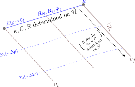
Figure 4: The constraint equations along with initial conditions on the horizon, i.e. $R_{\ell}\overset{\scriptscriptstyle{H}}{=}0,R_{N}\overset{\scriptscriptstyle{H}}{=}-1$ determine $\kappa$, $C$ and $R$ on $\bar{H}$

IV.3 Integrating from the final data

We now consider how that data can be integrated into the causal past of $\bar{H}\cup\bar{\mathcal{N}}$. The basic steps in the integration scheme are demonstrated in a simple numerical integration based on Euler approximations. This scheme alternates between using steps i)-v) to integrate data down the characteristics of constant $v$ followed by an application of (71) to calculate $\Phi_{N}$ on the next characteristic.

In more detail, assume a discretization $\{v_{m},\rho_{n}\}$ (with $m$ and $n$ at their maxima along the final surfaces) by steps $\Delta v$ and $\Delta\rho$. Then if all data is known along a surface $v_{m+1}$ and $R$ and $\Phi_{\ell}$ are known everywhere on $\bar{H}$:

1. Use the knowledge of $\Phi_{N}$ on $v_{m+1}$ to calculate $\Phi_{N,\rho}$.

2. Use (71) at $(v_{m},\rho_{n})$ to find $\Phi_{N,v}$. Then

   $$\Phi_{N}(v_{m},\rho_{n})\approx\Phi_{N}(v_{m+1},\rho_{n})-\Phi_{N,v}(v_{m+1},\rho_{n})\Delta v$$ (99)

3. Apply (97) to calculate $\kappa$ at $(v_{m},0)$.

4. Use (86)-(89) to integrate the values of $R_{N,\rho}$, $\kappa_{,\rho}$ and $\Phi_{\ell,\rho}$ out along the $v=v_{m}$ characteristic as for the initial data.

This can then be repeated marching all the way along $\bar{H}$ as shown in FIG.5.

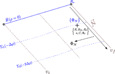
Figure 5: Evolving $\Phi$ in the $-\frac{\partial}{\partial v}$ direction.

This is how we would proceed for general cases. However those general studies will be left for a future paper. Here instead we will focus on spacetime near a slowly evolving horizon. There, as will be seen in the next section, $\Phi_{N,\rho}$ is negligible and it becomes possible to integrate along surfaces of constant $v$.

It may not be immediately obvious how this integration scheme obeys causality and what restricts it to determining points inside the domain of dependence. This is briefly discussed in Appendix A.

IV.4 Spacetime near a slowly evolving horizon

We now apply the formalism to a concrete example: weak scalar fields near the horizon. Physically the black hole will be close to equilibrium and hence the horizon slowly evolving in the sense of Booth and Fairhurst (2004, 2007).

“Near horizon” means that we expand all quantities as Taylor series in $\rho$ and keep terms up to order $\rho^{2}$. “Weak scalar field” means that we assume

$$\Phi_{N},\Phi_{\ell}\sim\frac{\varepsilon}{R}$$ (100)

and then expand the terms of the Taylor series up to order $\epsilon^{2}$. To order $\epsilon^{0}$ the spacetime will be vacuum (and Schwarzschild), order $\epsilon^{1}$ will be a test scalar field propagating on the Schwarzschild background and order $\epsilon^{2}$ will include the back reaction of the scalar field on the geometry.

IV.4.1 Expanding the equations

We expand all quantities as Taylor series in $\rho$. That is for $X\in\{R,R_{N},R_{\ell},\kappa,C,\Phi_{\ell},\Phi_{N}\}$

$$X(v,\rho)=\sum_{n=0}^{\infty}\frac{\rho^{n}X^{(n)}(v)}{n!}$$ (101)

with

$$R_{N}^{(n)}=R^{(n+1)}\;\;\mbox{and}\;\kappa^{(n)}=C^{(n+1)}\;.$$ (102)

The free final data is $\Phi_{\ell}^{(0)}$ on $\bar{H}$, $R_{o}$ on $\bar{H}\cap\bar{\mathcal{N}}$ and the Taylor expanded

$$\Phi_{N_{f}}(\rho)=\sum_{n=0}^{\infty}\frac{\rho^{n}}{n!}\Phi_{N_{f}}^{(n)}\,$$ (103)

on $\bar{\mathcal{N}}$. Following Frolov and Novikov (1998) we give names to special cases of this free data:

1. out-modes: no flux through $\bar{H}$ ($\Phi_{\ell}^{(0)}=0$),
   non-zero flux through $\bar{\mathcal{N}}$ ($\Phi^{(n)}_{N}\neq 0$ for some $n$)

2. down-modes: non-zero flux through $\bar{H}$ ($\Phi_{\ell}^{(0)}\neq 0$),
   zero flux through ${\bar{\mathcal{N}}}$ ($\Phi^{(n)}_{N}=0$ for all $n$)

From the free data we construct the rest of the final data on $\bar{H}$. Equations (93) and (97) give

$$C^{(0)} =2\Phi_{\ell}^{(0)^{\mbox{\scriptsize{2}}}}$$ (104)

$$C^{(1)} =\kappa^{(0)}\approx\frac{1}{2R^{(0)}}\,.$$ (105)

Here and in what follows the $\approx$ indicates that terms of order $\epsilon^{3}$ or higher have been dropped. Further by our gauge choice

$$R_{N}^{(0)}=R^{(1)}=-1$$ (106)

and so from (107)

$$R^{(0)}=R_{o}+\int_{v_{f}}^{v}\!\!C^{(0)}\,\mbox{d}v\,.$$ (107)

This is an order $\epsilon^{2}$ correction as long as the interval of integration is small relative to $\nicefrac{{1}}{{\epsilon}}$.

The last piece of final data on $\bar{H}$ is $\Phi_{N}^{(0)}$ and comes from the first order differential equation (95)

$$\frac{\mbox{d}\Phi_{N}^{(0)}}{\mbox{d}v}+\frac{\Phi_{N}^{(0)}}{2R_{o}}\approx\frac{\Phi_{\ell}^{(0)}}{R_{o}}\,$$ (108)

which has the solution

$$\Phi_{N}^{(0)}=\Phi_{N_{f}}^{(0)}e^{\nicefrac{{(v_{f}-v)}}{{2R_{o}}}}+e^{-\nicefrac{{v}}{{2R_{o}}}}\int_{v_{f}}^{v}e^{\nicefrac{{\tilde{v}}}{{2R_{o}}}}\Phi_{\ell}^{(0)}\mbox{d}\tilde{v}$$ (109)

in which the free data $\Phi_{N_{f}}^{(0)}$ came in as a boundary condition. Note that scalar fields that start small on the boundaries remain small in the interior, again as long as the integration time is short compared to $\nicefrac{{1}}{{\epsilon}}$. We assume that this is the case.

From the final data, the black hole is close to equilibrium and the horizon is slowly evolving to order $\epsilon^{2}$. That is, the expansion parameter Booth and Fairhurst (2004, 2007):

$$C\left(\frac{1}{2}\theta_{(N)}^{2}+G_{ab}N^{a}N^{b}\right)\approx\left(\frac{4\Phi_{\ell}^{2}}{R^{2}}\right)\sim\frac{4\epsilon^{2}}{R^{2}}\;.$$ (110)

Further we already have the first order expansion of $C$:

$$C\approx 2\Phi_{\ell}^{(0)^{\mbox{\scriptsize{2}}}}\!+\frac{\rho}{2R_{o}}\,.$$ (111)

That is (to first order) there is a null surface at

$$\rho_{\mbox{\tiny{EHC}}}\approx-4R_{o}\Phi_{\ell}^{(0)^{\mbox{\scriptsize{2}}}}\;.$$ (112)

This null surface is the event horizon candidate discussed in Booth (2013): if the horizon remains slowly evolving throughout its future evolution and ultimately transitions to isolation then the event horizon candidate is the event horizon.

Moving off the horizon to calculate up to second order in $\rho^{2}$, from (86) and (87) we find

$$R_{N}^{(1)}=R^{(2)} \approx-\frac{\Phi_{N}^{{(0)}^{\mbox{\scriptsize{2}}}}}{R_{o}}$$ (113)

$$R_{N}^{(2)} \approx-\frac{\Phi_{N}^{(0)}\left(\Phi_{N}^{(0)}+2R_{o}\Phi_{N}^{(1)}\right)}{R_{o}^{2}}\,$$ (114)

and so from (81)

$$R_{\ell}^{(0)} =0$$ (115)

$$R_{\ell}^{(1)} =-\frac{1}{2R^{(0)}}$$ (116)

$$R_{\ell}^{(2)} =-\frac{1}{R^{{(0)}^{\mbox{\scriptsize 2}}}}\,.$$ (117)

Note that the last two terms will include terms of order $\epsilon^{2}$ once the (107) integration is done to calculate $R^{(0)}$.

From (89) we can rewrite $\Phi_{\ell}^{(n)}$ terms with respect to $\Phi_{N}^{(n)}$ ones:

$$\Phi_{\ell}^{(1)} =0$$ (118)

$$\Phi_{\ell}^{(2)} \approx\frac{\Phi^{(0)}_{N}}{2R_{o}^{2}}\,.$$ (119)

The vanishing linear-order term reflects the fact that close to the horizon (where $R_{\ell}=0$) the inward flux decouples from the outward (89) and so freely propagates into the black hole. Physically this means that (to first order in $\rho$ near the horizon) the horizon flux is approximately equal to the “near-horizon” flux.

Next, from (88)

$$\kappa^{(1)} =C^{(2)}\approx\frac{1}{R^{{(0)}^{\mbox{\scriptsize 2}}}}-\frac{2\Phi_{\ell}^{(0)}\Phi_{N}^{(0)}}{R_{o}^{2}}\mbox{ and}$$ (120)

$$\kappa^{(2)} \approx\frac{3}{R^{{(0)}^{\mbox{\scriptsize 2}}}}-\frac{2\Phi_{\ell}^{(0)}\left(2\Phi_{N}^{(0)}+R_{o}\Phi_{N}^{(1)}\right)}{R_{o}^{2}}\,.$$ (121)

Again keep in mind that the $R^{(0)}$ terms will be corrected to order $\epsilon^{2}$ from (107).

Finally these quantities may be substituted into (71) to get differential equations for the $\Phi^{(n)}_{N}$:

$$\frac{\mbox{d}\Phi_{N}^{(1)}}{\mbox{d}v}+\frac{\Phi_{N}^{(1)}}{R_{o}} \approx\frac{\Phi_{\ell}^{(0)}}{R_{o}^{2}}-\frac{\Phi_{N}^{(0)}}{R_{o}^{2}}$$ (122)

$$\frac{\mbox{d}\Phi_{N}^{(2)}}{\mbox{d}v}+\frac{3\Phi_{N}^{(2)}}{2R_{o}} \approx\frac{2\Phi_{\ell}^{(0)}}{R_{o}^{3}}-\frac{5\Phi_{N}^{(0)}}{2R_{o}^{3}}-\frac{3\Phi_{N}^{(1)}}{R_{o}^{2}}\,.$$ (123)

Like (109) these are easily solved with an integrating factor and respectively have $\Phi_{N_{f}}^{(1)}$ and $\Phi_{N_{f}}^{(2)}$ as boundary conditions.

Note the important simplification in this regime that enables these straightforward solutions. The fact that $R_{\ell}\sim\rho$ has raised the $\rho$-order of the $\Phi_{N,\rho}$ terms. As a result we can integrate directly across the $\rho=\mbox{constant}$ surfaces rather than having to pause at each step to first calculate the $\rho$-derivative. The $\Phi_{N_{f}}^{(n)}$ are final data for these equations. They can be solved order-by-order and then substituted back into the other expressions to reconstruct the near-horizon spacetime.

It is also important that the matter and geometry equations decompose cleanly in orders of $\epsilon$: we can solve the matter equations at order $\epsilon$ relative to a fixed background geometry and then use those results to solve for the corrections to the geometry at order $\epsilon^{2}$.

IV.4.2 Constant inward flux

We now consider the concrete example of an affinely constant flux through $\bar{H}$ along with an analytic flux through $\bar{\mathcal{N}}$. Then by Appendix B

$$\Phi_{\ell}^{(0)}=\Phi_{\ell_{f}}^{(0)}{e}^{V}\,,$$ (124)

where $\Phi_{\ell_{f}}^{(0)}$ is the value of $\Phi_{\ell}^{(0)}$ at $v_{f}$ and $V=\frac{v-v_{f}}{2R_{o}}$ while $\Phi_{N_{f}}$ retains its form from (103).

We solve the equations for this data up to second order in $\rho$ and $\epsilon$. First for $\Phi_{N}^{(n)}$ equations we find:

$$\Phi_{N}^{(0)}\approx \;\left(e^{V}\!-e^{-V}\right)\Phi_{\ell_{f}}^{(0)}+e^{-V}\Phi_{N_{f}}^{(0)}$$ (125)

$$\Phi_{N}^{(1)}\approx \;\frac{2\Phi_{\ell_{f}}^{(0)}}{R_{o}}\left(1-e^{-2V}\right)+\frac{2\Phi_{N_{f}}^{(0)}}{R_{o}}\left(e^{-2V}-e^{-V}\right)$$ (126)

$$\!+\Phi_{N_{f}}^{(1)}e^{-2V}$$

$$\Phi_{N}^{(2)}\approx -\frac{\Phi_{\ell_{f}}^{(0)}}{4R_{o}^{2}}\left(e^{V}\!+14e^{-V}-48e^{-2V}\!+33e^{-3V}\right)$$ (127)

$$+\frac{\Phi_{N_{f}}^{(0)}}{2R_{o}^{2}}\left(7e^{-V}\!-24e^{-2V}+17e^{-3V}\right)$$

$$+\frac{6\Phi_{N_{f}}^{(1)}}{R_{o}}\left(e^{-3V}\!-e^{-2V}\right)+\Phi_{N_{f}}^{(2)}e^{-3V}$$ (128)

and so

$$\Phi_{\ell}^{(0)} =e^{V}\Phi_{\ell_{f}}^{(0)}\,$$ (129)

$$\Phi_{\ell}^{(1)} =0$$ (130)

$$\Phi_{\ell}^{(2)} \approx\frac{\Phi_{\ell_{f}}^{(0)}}{2R_{o}^{2}}\left(e^{V}\!-e^{-V}\right)+\frac{\Phi_{N_{f}}^{(0)}}{2R_{o}^{2}}e^{-V}\,.$$ (131)

The scalar field equations are linear and so it is not surprising that to this order in $\epsilon$ each solution can be thought of as a linear combination of down and out modes.

However for the geometry at order $\epsilon^{2}$, down and out modes no longer combine in a linear way. These quantities can be found simply by substituting the $\Phi_{\ell}^{(n)}$ and $\Phi_{N}^{(n)}$ into the expression for $R^{(n)}$, $R_{N}^{(n)}$, $R_{\ell}^{(n)}$, $C^{(n)}$ and $\kappa^{(n)}$ given in the last section. They are corrected at order $\epsilon^{2}$ by flux terms that are quadratic in combinations of $\Phi_{\ell_{f}}^{(m)}$ and $\Phi_{N_{f}}^{(n)}$. The terms are somewhat messy and the details not especially enlightening. Hence we do not write them out explicitly here.

IV.4.3 $\bar{H}-\bar{\mathcal{N}}$ correlations

From the preceding sections it is clear that there does not need to be any correlation between the scalar field flux crossing $\bar{H}$ and that crossing $\bar{\mathcal{N}}$. These fluxes are actually free data. Any correlations will result from appropriate initial configurations of the fields. In this final example we consider a physically interesting case where such a correlation exists.

Consider quadratic affine final data (Appendix B) on $\bar{H}=\{(v,0):v_{i}<v<v_{f}\}$:

$$\Phi_{\ell}^{(0)}=a_{0}e^{V}+a_{1}e^{2V}+a_{2}e^{3V}$$ (132)

for $V=\nicefrac{{v-v_{f}}}{{2R_{o}}}$ along with similarly quadratic affine data on $\bar{\mathcal{N}}$:

$$\Phi_{N_{f}}=\Phi_{N_{f}}^{(0)}+\rho\Phi_{N_{f}}^{(1)}+\frac{\rho^{2}}{2}\Phi_{N_{f}}^{(2)}.$$ (133)

A priori these are uncorrelated but let us restrict the initial configuration so that $\Phi_{N}^{(n)}(v_{i})=0$. That is, there is no $\Phi_{N}$ flux through $v=v_{i}$.

Then the process to apply these conditions is, given the free final data on $\bar{H}$:

1. Solve for the $\Phi_{N}^{(n)}$ from (108), (122) and (123).

2. Solve $\Phi_{N}^{(n)}(v_{i})=0$ to find the $\Phi_{N_{f}}^{(n)}$ in terms of the $a_{n}$. These are linear equations and so the solution is straightforward.

3. Substitute the resulting expressions for $\Phi_{N}^{(n)}$ into results from the previous sections to find all other quantities.

These calculations are straightforward but quite messy. Here we only present the final results for $\Phi_{N_{f}}$:

$$\Phi_{N_{f}}^{(0)}\approx (1\!-e^{2V_{i}})a_{0}+\frac{2a_{1}(1\!-e^{3V_{i}})}{3}+\frac{a_{2}(1\!-e^{4V_{i}})}{2}$$ (134)

$$\Phi_{N_{f}}^{(1)}\approx \frac{2a_{0}(e^{2V_{i}}-e^{3V_{i}})}{R_{o}}+\frac{a_{1}(1+8e^{3V_{i}}-9e^{4V_{i}})}{6R_{o}}$$ (135)

$$+\frac{a_{2}(1+5e^{4V_{i}}-6e^{5V_{i}})}{5R_{o}}$$

$$\Phi_{N_{f}}^{(2)}\approx -\frac{a_{0}(1+14e^{2V_{i}}-48e^{3V_{i}}+33e^{4V_{i}})}{4R_{o}^{2}}$$ (136)

$$-\frac{a_{1}(1+35e^{3V_{i}}-135e^{4V_{i}}+99e^{5V_{i}})}{15R_{o}^{2}}$$

$$+\frac{a_{2}(1-35e^{4V_{i}}+144e^{5V_{i}}-110e^{6V_{i}})}{20R_{o}^{2}}$$

where $V_{i}=V(v_{i})$. If $V_{i}$ is sufficiently negative that we can neglect the exponential terms:

$$\Phi_{N_{f}}^{(0)}\approx \;a_{0}+\frac{2a_{1}}{3}+\frac{a_{2}}{2}$$ (137)

$$\Phi_{N_{f}}^{(1)}\approx \frac{a_{1}}{6R_{o}}+\frac{a_{2}}{5R_{o}}$$

$$\Phi_{N_{f}}^{(2)}\approx -\frac{a_{0}}{4R_{o}^{2}}+-\frac{a_{1}}{15R_{o}^{2}}+\frac{a_{2}}{20R_{o}^{2}}\;.$$

In either case the flux through $\bar{H}$ fully determines the flux through $\bar{\mathcal{N}}$. The constraint at $v_{i}$ is sufficient to determine the Taylor expansion of the flux through $\bar{\mathcal{N}}$ relative to the expansion of the flux through $\bar{H}$. Though we only did this to second order in $\rho/v$ we expect the same process to fix the expansions to arbitrary order.

V Discussion

In this paper we have begun building a formalism that constructs spacetime in the causal past of a horizon $\bar{H}$ and an intersecting ingoing null surface $\bar{{\cal N}}$ using final data on those surfaces. It can be thought of as a specialized characteristic initial value formulation and is particularly closely related to that developed in Winicour (2013). Our main interest has been to use the formalism to better understand the relationship between horizon dynamics and off-horizon fluxes. So far we have restricted our attention to spherical symmetry and so included matter fields to drive the dynamics.

One of the features of characteristic initial value problems is that they isolate free data that may be specified on each of the initial surfaces. Hence it is no surprise that the corresponding data in our formalism is also free and uncorrelated. We considered two types of data: inward flowing null matter and massless scalar fields.

For the inward-flowing null matter, data on the horizon actually determines the entire spacetime running backwards along the ingoing null geodesics that cross $\bar{H}$. Physically this makes sense. This is the only flow of matter and so there is nothing else to contribute to the dynamics.

More interesting are the massless scalar field spacetimes. In that case, matter can flow both inwards and outwards and further inward moving radiation can scatter outwards and vice versa. For the weak field near-horizon regime that we studied most closely, the free final data is the scalar field flux through $\bar{H}$ and $\bar{\mathcal{N}}$ along with the value of $R$ at their intersection. Hence, as noted, these fluxes are uncorrelated. However we also considered the case where there was no initial flux of scalar field travelling “up” the horizon. In this case the coefficients of the Taylor expansion of the inward flux on $\bar{H}$ fully determined those on $\bar{\mathcal{N}}$ (though in a fairly complicated way). This constraint is physically reasonable: one would expect the dominant matter fields close to a black hole horizon to be infalling as opposed to travelling (almost) parallel to the horizon. It is hard to imagine a mechanism for generating strong parallel fluxes.

While we have so far worked in spherical symmetry the current work still suggests ways to think about the horizon-$\mathscr{I}^{+}$ correlation problem for general spacetimes. For a dynamic non-spherical vacuum spacetime, gravitational wave fluxes will be the analogue of the scalar field fluxes of this paper and almost certainly they will also be free data. Then any correlations will necessarily result from special initial configurations. However as in our example these may not need to be very exotic. It may be sufficient to eliminate strong outward-travelling near horizon fluxes. In future works we will examine these more general cases in detail.

Appendix A Causal past of $\bar{H}\cup\bar{\cal{N}}$

In this appendix we consider how the general integration scheme for the scalar field spacetimes of Section IV “knows” how to stay within the past domain of dependence of $\bar{H}\cup\bar{\mathcal{N}}$.

Figure 6: Causality restrictions on $\Delta v$: the CFL condition restricts the choice of $\Delta v$ to ensure that attempted numerical evolutions respect causality. In this figure the $\rho$ and $v$ coordinates are drawn to be perpendicular to clarify the connection with the usual advection equation: to compare to other diagrams rotate about $45^{\circ}$ clockwise and skew so coordinate curves are no longer perpendicular. The dashed lines are null and have slope $C$ in this coordinate system. If data at points $A$, $B$ and $C$ are used to determine $\Phi_{N,\rho}$ then the size of the discrete $v$-evolution is limited to lie inside the null line from point $C$. The largest $\Delta v$ allowed by the restriction evolves to $D$.

First, it is clear how the process develops spacetime up to the bottom left-hand null boundary ($v=v_{i}$) of the past domain of dependence. The bottom right-hand boundary is a little more complicated but follows from the advection form of the $\Phi_{N,v}$ equation (74). Details will depend on the exact numerical scheme but the general picture is as follows.

Assume that we have discretized the problem so that we are working at points $(v_{j},\rho_{k})$. Then in using (74) to move from a surface $v_{i}$ to $v_{i-1}$, the Courant-Friedrichs-Lewy (CFL) condition (common to many hyperbolic equations) tells us that the maximum allowed $\Delta v$ is

$$\Delta v<\frac{\Delta\rho}{C}\,,$$ (138)

where $\Delta\rho$ is the coordinate separation of the points that we are using to calculate the right-hand side of (74).

Then, as shown in FIG. 6, the discretization progressively loses points of the bottom right of the diagram: they are outside of the domain of dependence of the individual points being used to determine them. For example if we are using a centred derivative so that

$$\Phi_{N,\rho}\approx\frac{\Phi_{N}(v_{j},\rho_{k+1})-\Phi_{N}(v_{j},\rho_{k-1})}{2\Delta\rho}$$ (139)

then we need adjacent points as shown in FIG. 6.

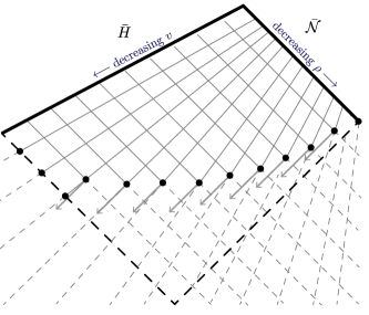
Figure 7: A cartoon showing the CFL-limited past domain of dependence of $\bar{H}\cup\bar{\mathcal{N}}$. Null lines are now drawn at $45^{\circ}$ so the analytic past domain of dependence is bound by the heavy dashed null lines running back from the ends of $\bar{H}$ and $\bar{\mathcal{N}}$. A (very coarse) discretization is depicted by the gray lines and the region that cannot be determined with dashed lines. The boundary points of that region are heavy dots.

The lower-right causal boundary of FIG. 1 is then enforced by a combination of the endpoints of $\bar{\mathcal{N}}$ and the CFL condition as shown in FiG. 7. Points are progressively lost as they require greater than the maximum allowed $\Delta v$. The numerical past-domain of dependence necessarily lies inside the analytic domain. The coarseness of the discretization in the figure dramatizes the effect: a finer discretization would keep the domains closer.

Appendix B Affine derivatives and final data

The off-horizon $\rho$-coordinate in our coordinate system is affine while $v$ is not. However, as seen in the main text, when considering the final data on $\bar{H}$ it is more natural to work relative to an affine parameter. This is somewhat complicated because $\Phi_{\ell}$ and $\Phi_{N}$ are respectively linearly dependent on $\ell$ and $N$ and the scaling of those vectors is also tied to coordinates via (1), (2) and (6). In this appendix we will discuss the affine parameterization of the horizon and the associated affine derivatives for various quantities.

Restricting our attention to an isolated horizon $\bar{H}$ with $\kappa=\frac{1}{2R_{o}}$, consider a reparameterization

$$\tilde{v}=\tilde{v}(v)\,.$$ (140)

Then

$$\frac{\partial}{\partial v}=\frac{\mbox{d}\tilde{v}}{\mbox{d}v}\frac{\partial}{\partial\tilde{v}}$$ (141)

and so

$$\ell=e^{V}\tilde{\ell}\;\;\mbox{and}\;N=e^{-V}\tilde{N}$$ (142)

where we have defined $V$ so that $\displaystyle e^{V}=\frac{\mbox{d}\tilde{v}}{\mbox{d}v}\,.$ Hence

$$\tilde{\kappa}=-\tilde{N}_{b}\tilde{\ell}^{a}\nabla_{a}\tilde{\ell}^{b}=e^{-V}\left(\kappa-\frac{\mbox{d}V}{\mbox{d}v}\right)\,$$ (143)

and so for an affine parameterization ($\kappa=\partial_{v}V$):

$$e^{V}=\exp\left(\frac{v-v_{f}}{2R_{o}}\right)$$ (144)

for some $v_{f}$ and

$$\tilde{v}-\tilde{v}_{o}=2R_{o}e^{V}$$ (145)

for some $\tilde{v}_{o}$. The $v_{f}$ freedom corresponds to the freedom to rescale an affine parameterization by a constant multiple while the $\tilde{v}_{o}$ is the freedom to set the zero of $\tilde{v}$ wherever you like.

Now consider derivatives with respect to this affine parameter. For a regular scalar field

$$\frac{\mbox{d}f}{\mbox{d}\tilde{v}}=e^{-V}\frac{\mbox{d}f}{\mbox{d}v}\,.$$ (146)

However in this paper we are often interested in scalar quantities that are defined with respect to the null vectors:

$$\Phi^{(0)}_{\ell}=e^{V}\Phi^{(0)}_{\tilde{\ell}}\;\;\mbox{and}\;\Phi^{(0)}_{N}=e^{-V}\Phi^{(0)}_{\tilde{N}}\,.$$ (147)

Then

$$\frac{\mbox{d}\Phi^{(0)}_{\tilde{\ell}}}{\mbox{d}\tilde{v}}\! =\!e^{-V}\!\frac{\mbox{d}}{\mbox{d}v}\left(e^{-V}\Phi^{(0)}_{\ell}\!\right)\!=\!e^{-2V}\!\!\left(\!\frac{\mbox{d}\Phi^{(0)}_{\ell}}{\mbox{d}v}\!-\kappa\Phi^{(0)}_{\ell}\!\!\right)$$ (148)

$$\frac{\mbox{d}\Phi^{(0)}_{\!\tilde{N}}}{\mbox{d}\tilde{v}}\! =e^{-V}\!\frac{\mbox{d}}{\mbox{d}v}\left(e^{V}\Phi^{(0)}_{N}\right)=\frac{\mbox{d}\Phi^{(0)}_{N}}{\mbox{d}v}\!+\kappa\Phi^{(0)}_{N}\,.$$ (149)

That is these quantities are affinely constant if

$$\Phi_{\ell}=e^{V}\Phi^{(0)}_{\ell_{f}}\;\;\mbox{and}\;\Phi_{N}=e^{-V}\Phi^{(0)}_{N_{f}}$$ (150)

for some constants $\Phi^{(0)}_{\ell_{f}}$ and $\Phi^{(0)}_{N_{f}}$.

In the main text we write this affine derivative on $\bar{H}$ as $D_{v}$ with its exact form depending on the $\ell$ or $N$ dependence of the quantity being differentiated.

Finally at (132) we consider a $\Phi_{\ell}$ that is “affinely quadratic”. By this we mean that:

$$\Phi_{\tilde{\ell}} =A_{o}+A_{1}\tilde{v}+A_{2}\tilde{v}^{2}$$

$$\mspace{70.0mu}\Updownarrow$$

$$\Phi_{\ell} =a_{o}e^{V}+a_{1}e^{2V}+a_{2}e^{3V}\,,$$ (151)

where for simplicity we have set $\tilde{v}_{o}$ to zero (so that $v=0$ is $\tilde{V}=2R_{o}$) and absorbed the extra $2R_{o}$s into the $a_{n}$.

References

- https://www.black holes.org (2018) https://www.black holes.org, “Simulating extreme spacetimes,” (2018).
- Hawking and Ellis (2011) S. W. Hawking and G. F. R. Ellis, The Large Scale Structure of Space-Time, Cambridge Monographs on Mathematical Physics (Cambridge University Press, 2011).
- Thorne et al. (1986) Kip S. Thorne, R.H. Price, and D.A. Macdonald, Black holes: the membrane paradigm, edited by Kip S. Thorne (Yale University Press, 1986).
- Jaramillo et al. (2012a) Jose Luis Jaramillo, Rodrigo Panosso Macedo, Philipp Moesta, and Luciano Rezzolla, “Black-hole horizons as probes of black-hole dynamics I: post-merger recoil in head-on collisions,” Phys. Rev. D85, 084030 (2012a), arXiv:1108.0060 [gr-qc] .
- Jaramillo et al. (2012b) Jose Luis Jaramillo, Rodrigo P. Macedo, Philipp Moesta, and Luciano Rezzolla, “Black-hole horizons as probes of black-hole dynamics II: geometrical insights,” Phys. Rev. D85, 084031 (2012b), arXiv:1108.0061 [gr-qc] .
- Jaramillo et al. (2011) J. L. Jaramillo, R. P. Macedo, P. Moesta, and L. Rezzolla, “Towards a cross-correlation approach to strong-field dynamics in Black Hole spacetimes,” Proceedings, Spanish Relativity Meeting : Towards new paradigms. (ERE 2011): Madrid, Spain, August 29-September 2, 2011, AIP Conf. Proc. 1458, 158–173 (2011), arXiv:1205.3902 [gr-qc] .
- Rezzolla et al. (2010) Luciano Rezzolla, Rodrigo P. Macedo, and Jose Luis Jaramillo, “Understanding the ’anti-kick’ in the merger of binary black holes,” Phys. Rev. Lett. 104, 221101 (2010), arXiv:1003.0873 [gr-qc] .
- Gupta et al. (2018) Anshu Gupta, Badri Krishnan, Alex Nielsen, and Erik Schnetter, “Dynamics of marginally trapped surfaces in a binary black hole merger: Growth and approach to equilibrium,” Phys. Rev. D97, 084028 (2018), arXiv:1801.07048 [gr-qc] .
- Griffiths and Podolsky (2009) Jerry B. Griffiths and Jiri Podolsky, Exact Space-Times in Einstein’s General Relativity, Cambridge Monographs on Mathematical Physics (Cambridge University Press, Cambridge, 2009).
- Ashtekar et al. (2000a) Abhay Ashtekar, Christopher Beetle, Olaf Dreyer, Stephen Fairhurst, Badri Krishnan, Jerzy Lewandowski, and Jacek Wisniewski, “Isolated horizons and their applications,” Phys. Rev. Lett. 85, 3564–3567 (2000a), arXiv:gr-qc/0006006 [gr-qc] .
- Hayward (1994a) S.A. Hayward, “General laws of black hole dynamics,” Phys.Rev. D49, 6467–6474 (1994a).
- Ashtekar et al. (1999) Abhay Ashtekar, Christopher Beetle, and Stephen Fairhurst, “Isolated horizons: A Generalization of black hole mechanics,” Class. Quant. Grav. 16, L1–L7 (1999), arXiv:gr-qc/9812065 [gr-qc] .
- Ashtekar et al. (2000b) Abhay Ashtekar, Christopher Beetle, and Stephen Fairhurst, “Mechanics of isolated horizons,” Class. Quant. Grav. 17, 253–298 (2000b), arXiv:gr-qc/9907068 [gr-qc] .
- Hayward (1994b) Sean A. Hayward, “General laws of black-hole dynamics,” Phys. Rev. D 49, 6467–6474 (1994b).
- Ashtekar and Krishnan (2003) Abhay Ashtekar and Badri Krishnan, “Dynamical horizons and their properties,” Phys. Rev. D68, 104030 (2003), arXiv:gr-qc/0308033 [gr-qc] .
- Bousso and Engelhardt (2015) Raphael Bousso and Netta Engelhardt, “Proof of a New Area Law in General Relativity,” Phys. Rev. D92, 044031 (2015), arXiv:1504.07660 [gr-qc] .
- Booth and Fairhurst (2004) Ivan Booth and Stephen Fairhurst, “The First law for slowly evolving horizons,” Phys. Rev. Lett. 92, 011102 (2004), arXiv:gr-qc/0307087 [gr-qc] .
- Baumgarte and Shapiro (2010) Thomas W. Baumgarte and Stuart L. Shapiro, Numerical Relativity: Solving Einstein’s Equations on the Computer (Cambridge University Press, 2010).
- Thornburg (2007) Jonathan Thornburg, “Event and apparent horizon finders for 3+1 numerical relativity,” Living Rev. Rel. 10, 3 (2007), arXiv:gr-qc/0512169 [gr-qc] .
- Dreyer et al. (2003) Olaf Dreyer, Badri Krishnan, Deirdre Shoemaker, and Erik Schnetter, “Introduction to isolated horizons in numerical relativity,” Phys. Rev. D67, 024018 (2003), arXiv:gr-qc/0206008 [gr-qc] .
- Cook and Whiting (2007) Gregory B. Cook and Bernard F. Whiting, “Approximate Killing Vectors on S**2,” Phys. Rev. D76, 041501 (2007), arXiv:0706.0199 [gr-qc] .
- Chu et al. (2011) Tony Chu, Harald P. Pfeiffer, and Michael I. Cohen, “Horizon dynamics of distorted rotating black holes,” Phys. Rev. D83, 104018 (2011), arXiv:1011.2601 [gr-qc] .
- Lovelace et al. (2015) Geoffrey Lovelace et al., “Nearly extremal apparent horizons in simulations of merging black holes,” Class. Quant. Grav. 32, 065007 (2015), arXiv:1411.7297 [gr-qc] .
- Owen et al. (2017) Robert Owen, Alex S. Fox, John A. Freiberg, and Terrence Pierre Jacques, “Black Hole Spin Axis in Numerical Relativity,” (2017), arXiv:1708.07325 [gr-qc] .
- Rendall (1990) A. D. Rendall, “Reduction of the characteristic initial value problem to the Cauchy problem and its applications to the Einstein equations,” Proc. Roy. Soc. London Ser. A 427, 221–239 (1990).
- Sachs (1962) R. K. Sachs, “On the characteristic initial value problem in gravitational theory,” Journal of Mathematical Physics 3, 908–914 (1962), https://doi.org/10.1063/1.1724305 .
- Winicour (2012) Jeffrey Winicour, “Characteristic Evolution and Matching,” Living Rev. Rel. 15, 2 (2012).
- Winicour (2013) J. Winicour, “Affine-null metric formulation of Einstein’s equations,” Phys. Rev. D87, 124027 (2013), arXiv:1303.6969 [gr-qc] .
- Mädler and Winicour (2016) Thomas Mädler and Jeffrey Winicour, “Bondi-Sachs Formalism,” Scholarpedia 11, 33528 (2016), arXiv:1609.01731 [gr-qc] .
- Li and Lucietti (2016) Carmen Li and James Lucietti, “Transverse deformations of extreme horizons,” Class. Quant. Grav. 33, 075015 (2016), arXiv:1509.03469 [gr-qc] .
- Li and Lucietti (2018) Carmen Li and James Lucietti, “Electrovacuum spacetime near an extreme horizon,” (2018), arXiv:1809.08164 [gr-qc] .
- Krishnan (2012) Badri Krishnan, “The spacetime in the neighborhood of a general isolated black hole,” Class. Quant. Grav. 29, 205006 (2012), arXiv:1204.4345 [gr-qc] .
- Lewandowski and Li (2018) Jerzy Lewandowski and Carmen Li, “Spacetime near Kerr isolated horizon,” (2018), arXiv:1809.04715 [gr-qc] .
- Booth (2013) Ivan Booth, “Spacetime near isolated and dynamical trapping horizons,” Phys. Rev. D87, 024008 (2013), arXiv:1207.6955 [gr-qc] .
- Booth and Fairhurst (2007) Ivan Booth and Stephen Fairhurst, “Isolated, slowly evolving, and dynamical trapping horizons: Geometry and mechanics from surface deformations,” Phys. Rev. D75, 084019 (2007), arXiv:gr-qc/0610032 [gr-qc] .
- Booth et al. (2006) Ivan Booth, Lionel Brits, Jose A. Gonzalez, and Chris Van Den Broeck, “Marginally trapped tubes and dynamical horizons,” Class. Quant. Grav. 23, 413–440 (2006), arXiv:gr-qc/0506119 [gr-qc] .
- Frolov and Novikov (1998) V. P. Frolov and I. D. Novikov, eds., Black hole physics: Basic concepts and new developments, Vol. 96 (1998).