On the primordial specific frequency of globular clusters in dwarf and giant elliptical galaxies
Abstract
Globular clusters (GC) are important objects for tracing the early evolution of a galaxy. We study the relation between the properties of globular cluster systems - as quantified by the GC specific frequency () - and the properties of their host galaxies. In order to understand the origin of the relation between the GC specific frequency () and galaxy mass, we devise a theoretical model for the specific frequency (). GC erosion is considered to be an important aspect for shaping this relation, since observations show that galaxies with low densities have a higher , while high density galaxies have a small . We construct a model based on the hypothesis that star-formation is clustered and depends on the minimum embedded star cluster mass (), the slope of the power-law embedded cluster mass function () and the relation between the star formation rate (SFR) and the maximum star cluster mass (). We find an agreement between the primordial value of the specific frequency () and our model for between 1.5 and 2.5 with .
keywords:
galaxies : elliptical – globular cluster : specific frequency – number of globular clusters.1 Introduction
Globular clusters (GCs) are collisional stellar-dynamical near-spherical systems of stars and among the first stellar systems to form in the early Universe. GCs are found within different morphological types of galaxies, from irregular to spiral and elliptical galaxies. Most of the GCs appear to have formed within a few Gyr after the Big Bang (Gratton et al. 2003) and the properties of GC systems can be considered as important tracers for the formation and evolution of galaxies.
One of the basic parameters to describe the globular cluster system of a galaxy is the specific frequency, , which is the number of globular clusters, , divided by the -band luminosity of the galaxy, normalized at an absolute magnitude of the galaxy in the -band () of -15 mag (Harris & van den Bergh 1981):
| (1) |
The specific frequency measures the richness of a GC system and varies between galaxies of different morphological types: is smaller in late-type spiral galaxies than in early-type elliptical (E) galaxies (e.g Miller et al. 1998). Spiral galaxies have a between 0.5 and 2 (Goudfrooij et al. 2003; Chandar et al. 2004; Rhode et al. 2007). For more luminous elliptical galaxies, ranges from about 2 to 10 and tends to increase with luminosity, while increases from a few to several dozen with decreasing galaxy luminosity for dE galaxies that posses GCs (Miller & Lotz 2007; Peng et al. 2008; Georgiev et al. 2010). This difference in between types of galaxies needs to be understood in terms of formation models of galaxies (Beasley et al. 2002).
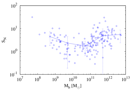
The relation between and total mass of a galaxy () reveals a ‘U’ -shape, i.e., higher for dwarfs galaxies and giant ellipticals (low and high- mass end of the scale, respectively), with a minimum for galaxies at an intermediate mass, as shown in Figure (1) (Harris et al. 2013).
There are many suggestions to explain the observed ‘U’ -shaped relation between and of the host galaxy. Forte et al. (1982) proposed a tidal stripping model of GCs from smaller galaxies to explain the increasing value of in cD galaxies (dominant ellipticals in the centers of clusters) and studies of the GC system around cD galaxies also supported this scenario (Forbes et al. 1997; Neilsen et al. 1997). Schweizer (1987) and Ashman & Zepf (1992) suggested elliptical galaxies formed from the mergers of spiral galaxies and lead to GC formation with a high efficiency which reflects the low of giant spiral galaxies.
Georgiev et al. (2010) investigated the trend of increasing above and below the absolute galaxy magnitude of mag and explain this trend by a theoretical model of GC specific frequency as a function of host galaxy dark matter halo mass with a universal specific GC formation efficiency . This is the total mass of GCs divided by the mass of the host dark matter halo, irrespective of galaxy morphology and which has a mean value of . Wu & Kroupa (2013) studied the apparent or phantom virial mass () of dark matter halos in Milgromian dynamics. They found and to be functions of . The number of GCs and increase for and decreases for .
Another ansatz to explain this ‘U’ -shape is for galaxies with a small and large mass to have been very inefficient at forming stars. Harris et al. (2013) suggested these galaxies formed their globular clusters before any other stars, then had a star formation shut off. Star formation is likely regulated by supernova feedback and virial shock-heating of the infalling gas for low and massive galaxies respectively, while intermediate mass galaxies have a maximum star formation efficiency (Dekel & Birnboim 2006).
GC destruction can be important for the relation between and (Mieske et al. 2014). Tidal erosion together with dynamical friction on the stellar component in different galaxies could produce different GC survival fractions, which may explain the present-day dependence of (cf with Mieske et al. 2014). Lamers et al. (2017) argue that is also consistently a strong function of metallicity.
In this paper, we present a model for the specific frequency of GCs. It is based on the notion that star formation occurs in correlated star formation events which arise in the density peaks in the molecular clouds that condense from the galaxy’s interstellar medium (ISM). These are spatially and temporally correlated with scales 1 pc and formation durations 1 Myr and can also be referred to as being embedded clusters.
This paper is organized as follows: in Section 2 we review that is reduced through erosion processes suggesting to be nearly constant. In Section 3 we determine the star cluster mass function population time-scales and the most-massive-cluster – SFR relation. The theoretical model of the specific frequency of globular clusters () is then presented in Section 4, which is based on the notion that star clusters are the basic building blocks of a galaxy (Kroupa 2005). Finally, Section 5 contains the conclusion.
2 GC populations and tidal erosion
The specific frequency of GCs () is an important tool to understand the evolution of galaxies (Harris 1991; Brodie & Strader 2006).
In this work, the data is taken from the Harris catalogue (Harris et al. 2013). We selected elliptical galaxies with masses ranging between and (with the exception of M32). These masses are dynamical masses of the galaxy, , where [pc Myr-1] is the velocity dispersion, [pc] the effective half light radius, and is the gravitational constant [ pc Myr-2]. We refer to these masses as total masses (), since the putative dark-matter halo has a small contribution to the mass within this radius (e.g. Graves & Faber 2010; Tiret et al. 2011; Harris et al. 2013; Smith & Lucey 2013), and stellar remnants from a top-heavy integrated galactic stellar initial mass function (IGIMF) account for this contribution (Weidner et al. 2013).
Figure (1) demonstrates a ‘U’ -shape relation between (calculated using equation 1) and (Harris et al. 2013). Mieske et al. (2014) explained this relation as an effect of tidal erosion. For the purpose of understanding how tidal erosion contributes to this relation, one has to study the relation between the 3D mass density () [pc3] within the half-light radius (3D half mass radius 1.35 times the projected half light radius) and [].
The relation between the 3D mass density and the total mass takes the same trend as the vs. relation as shown by Mieske et al. (2014). Near = is the highest mean density, while the density is lower for less and more massive galaxies. Galaxies with different densities appear to generate different GC survival times.
Mieske et al. (2014) arrived at two equations to calculate the GC survival fraction, , for initially isotropic () and radially anisotropic () GC orbital velocity distributions respectively. After 10 Gyr of evolution, GCs more massive than will have:
| (2) |
| (3) |
According to equations (2) and (3), more GCs get destroyed at higher densities for an initially radially anisotropic velocity distribution function.
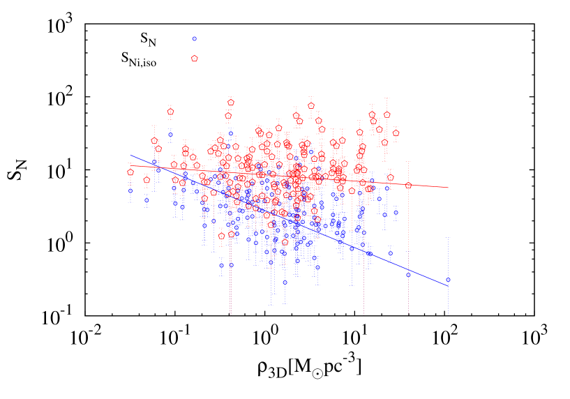
The correlation between the and is determined observationally: Figure (2) shows the observed present-day GC specific frequency and for the same sample as in Figure (1), which supports a high erosion of GCs at higher densities. The solid blue line is the bi-variate best fit to the observed data:
| (4) |
This supports the notion that the survival fractions of GCs may be an important aspect of the ‘U’ -shaped relation between and as suggested by Mieske et al. (2014).
In order to estimate the primordial value of the specific frequency, , for both cases, isotropic, , and radially anisotropic GC velocity distributions, , we divide by and by , respectively,
| (5) |
| (6) |
The primordial and the observed present-day specific frequency at different densities are illustrated in Figure (2). As already concluded by Mieske et al. (2014) it emerges that the initial specific frequency () is largely independent of . This result has potentially very important implication for our understanding of early galaxy assembly: being nearly constant with density, the efficiency of forming young GCs (i.e. the number of young clusters per mass) is about the same for all present-day early- type galaxies from dEs to Es, suggesting that the same fundamental principle was active, independent of the mass of the galaxy.
The primordial values of the number of globular clusters for the isotropic, , and anisotropic, , cases is calculated by dividing the observed number of globular clusters by the GC survival fractions and , respectively,
| (7) |
| (8) |
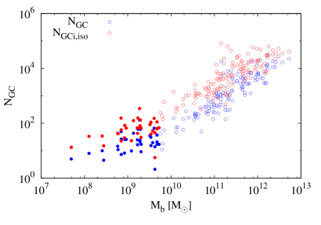
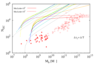
The primordial number of GCs increases monotonically with host galaxy mass. Figure (3) shows this relation for (red pentagons) and (blue circles) as a function of . Filled symbols are galaxies with a mass smaller than denoted by branch I (BI), while open symbols are galaxies with a mass larger than denoted by branch II (BII). Galaxies in branch I are dEs, while E galaxies are in branch II (Dabringhausen et al. 2008). The present-day number of GCs, , is lower than , especially for galaxies at intermediate-mass, because of the high destruction rates of GCs.
We now make the following ansatz: if the fundamental physical processes acting during the assembly of dE and E galaxies were the same, the former formed fewer GCs because their SFRs were much smaller than during the formation of E galaxies (Weidner et al. 2004; Randriamanakoto et al. 2013; Weidner et al. 2013). This ansatz is followed through a model in the next section.
3 The - correlation and the star cluster mass function population time-scale ()
An empirical relation has been derived by Recchi et al. (2009) for dE and E galaxies between the central velocity dispersion [km/s], which reflects the total stellar mass, and the stellar alpha-element abundance [/Fe]. The implied star formation duration, [yr], over which the galaxy assembled, inversely correlates with the mass [] of the galaxy (this is referred to as downsizing, see also Thomas et al. 1999),
| (9) |
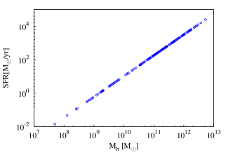
Knowing the total mass of a galaxy, , and , the star formation rate (SFR) follows as illustrated in Figure (4),
| (10) |
The time during which GCs formed () is part of the time scale of star formation in galaxies (), . Each part is divided into star cluster-population formation epochs of equal length , which we will calculate later (Figure 6). Assuming that all the stars form in embedded star clusters (Lada & Lada 2003; Kroupa 2005; Megeath et al. 2016), the total mass of the star cluster system formed during (), can be calculated using the SFR and ,
| (11) |
Observational studies suggest that the masses of young and embedded star-clusters are distributed as a power law:
| (12) |
where is the mass distribution function of the embedded clusters, is a normalization constant and is the stellar mass of the embedded cluster. The power law slope is found to be between 1.2 and 2.5 (Elmegreen & Efremov 1997; Lada & Lada 2003; Kroupa & Weidner 2003; Weidner et al. 2004; Whitmore et al. 2010; Chandar et al. 2011).
The total mass of a population of star clusters, , assembled within the time span can also be expressed as follows
| (13) |
where is the minimum mass of a star cluster and is the maximum star cluster mass depending on the SFR (Weidner et al. 2004). can be assumed to be 5 , which is about the lowest mass cluster observed to form in the nearby Taurus-Auriga aggregate (Briceño et al. 2002; Kroupa & Bouvier 2003; Weidner et al. 2004).
In order to determine the normalization constant in equation (12) we use the same assumption as in Weidner et al. (2004), that is the single most massive cluster formed in time . For and (equation 15 undefined) we get
|
||||
|---|---|---|---|---|
| 1.2 | 0.08 | 1.78 | ||
| 1.5 | 0.16 | 1.76 | ||
| 1.7 | 0.29 | 1.69 | ||
| 1.9 | 0.69 | 1.53 | ||
| 2.1 | 2.30 | 1.47 | ||
| 2.3 | 11.00 | 1.33 | ||
| 2.5 | 64.20 | 2.33 |
| (14) |
and equation (13) becomes,
| (15) |
In order to determine we correlate the theoretical upper mass limit of the star clusters and the most massive star cluster, using the same criteria as Schulz et al. (2015), which requires only one most massive cluster to exist (, where the theoretical upper mass limit, () ).
According to the conditions above and by combining equation (11) and (15) we obtain a relation between the SFR and for and :
| (16) |
with .
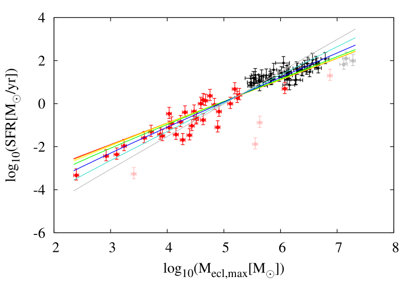
Observations indeed indicate that young massive star clusters follow a relation between the visual absolute magnitude of the brightest young cluster and the global SFR of the host galaxy (Larsen 2002). Based on this evidence Weidner et al. (2004) found a relation between the galaxy-wide SFR and the maximum star-cluster mass. As indicated in equation (11) the total mass depends on the current SFR at a certain , such that depends on the SFR (equation 16), which has also been determined observationally (Larsen & Richtler 2000; Weidner et al. 2004). It follows that galaxies with a high SFR are forming high-mass clusters.
The resulting relation between the SFR and the mass of the most massive cluster is illustrated in Figure (6). The data are from Weidner et al. (2004) and Randriamanakoto et al. (2013). Randriamanakoto et al. (2013) provide -band magnitudes which we converted to -band magnitudes using the colour-magnitude relation 111Randriamanakoto et al. (2013) use this relation to convert the data from Weidner et al. (2004) to the -band. It is also roughly the colour of a yr old population with solar metallicity (Bruzual & Charlot 2003).. We converted the luminosity of the brightest star cluster in the -band to the most massive star-cluster mass using equation (5) from Weidner et al. (2004). We used these data to determine the length of the formation epoch . The uncertainties in SFR were obtained from the uncertainties in conversion of the IR luminosity to a SFR. On the other hand the uncertainties in come from uncertainties in the conversion of luminosities to masses.
We exclude seven galaxies (faded colors) in Figure (6) from this population: The first four galaxies (in increasing values) are excluded since the SFRs of these dwarf galaxies do not represent the birth of these clusters (further details can be found in Weidner et al. 2004; Schulz et al. 2015). The last three galaxies (gray) have a luminosity distance from the NED database larger than 150 Mpc. Randriamanakoto et al. (2013) suggested that these brightest super star clusters might be a blend of many clusters.
The cluster-system mass function population time-scale, or the duration of the star formation ‘epoch’, , is determined by fitting equation (16) for = 1.2 - 2.5 to the data (Figure 6). The best value of as a function of is determined by the reduced chi-squared statistic . As can be seen in Table 1 and Figure (6), increases with . This result agrees with Schulz et al. (2015), who found by comparison with the literature that lies between 1.8 and 2.4. Also it is consistent with the analysis by Weidner et al. (2004). is minimized for , yr as already noted by Weidner et al. (2004). The typical time-scale of about yr has also been deduced from calculations of the Jeans time in molecular clouds (e.g. Egusa et al. 2004). The star formation time-scale can also be determined from examining offsets between and arms of a spiral galaxy as proposed by Egusa et al. (2009), who found the star formation time to be between 4 and 13 Myr. Independently of these arguments, Fukui & Kawamura (2010) review molecular cloud formation and find that on a time scale of 20-30 Myr the interstellar medium completes a cycle through the molecular phase with embedded star formation. This time scale is verified by Meidt et al. (2015). These time scale constraints are well consistent with Myr required to best match the data in Figure (6). We thus assume that every Myr a new population of star clusters hatches from the ISM of a star forming galaxy, follow the embedded cluster mass function (ECMF).
4 Theoretical specific frequency
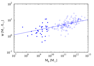
With equation (1), we can now derive an analytical model for , which is the theoretical number of globular clusters, , per unit galaxy luminosity in the V-band. The galaxy luminosity can be converted into a mass such that:
| (17) |
where is the stellar mass-to-light ratio of the galaxy in the appropriate photometric band. Figure (7) shows for the photometric band by using the same sample as in Figure (1). The best least square fit suggests,
| (18) |
with a = 0.80 0.13 and b = 0.15 0.01.
In order to estimate from equation (17), the number of globular clusters () is required. The GCs which formed during can be calculated using the ECMF,
| (19) |
to give
| (20) | ||||
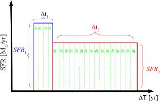
Note the difference between in equation (15) and in equation (20), since is the physical lower limit for the embedded cluster mass (Weidner & Kroupa 2004). From the SFR - relation (equation 16) and to calculate we assume two cases of SFR: in case one the SFR is constant and equal over the time scales , and ; in case two the SFR is not equal in the time scale and . While SFR1 is constant for t=t∘ until t=t and SFR2 is constant for t=(t) until t=(t). The minimum mass of clusters () which become after a few Gyr globular cluster is assumed to be and .
4.1 Constant and equal SFR over , and
In order to calculate the maximum mass of the old cluster systems in a galaxy , i.e., the clusters formed in the time span , we assume that the young stars formed in embedded clusters in time and the old cluster population formed with the same star-formation time scale, , which depends on for consistency with the data in Figure (6). That is, here we assume and that the whole galaxy including GCs formed during (i.e ). From this assumption for each galaxy in our sample we calculate the maximum masses of the old cluster systems at a given SFR (equation 16). In this model the SFR is supposed to be constant over different time scales, i.e., for , .
Having obtained and and using in the - band from equation (18), we can compute . By correcting the observed (equation 7) and (equation 5) for the erosion of GCs through tidal action or through dynamical friction, we obtain an estimate of the primordial values for each galaxy in our sample (as in Section 2).
4.1.1 Comparison between the theoretical model and primordial value of and
We investigate the influence of the two parameters and on and for each galaxy. For this purpose, we calculate the model for seven values of (1.2, 1.5, 1.7, 1.9, 2.1, 2.3 and 2.5), and for four different values of (, and ).
Since the overall distribution of and is similar (Mieske et al. 2014), we present the model only for the isotropic case.
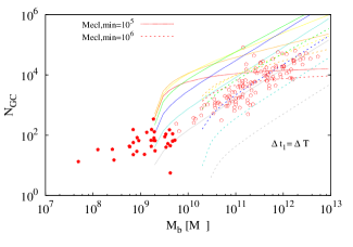
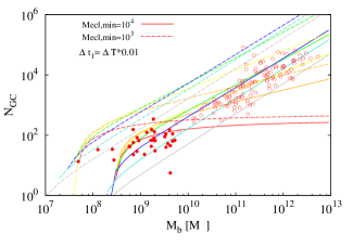
The E and dE galaxies formed under different physical boundary conditions (Okazaki & Taniguchi 2000; Dabringhausen & Kroupa 2013), which need different formation time-scales. We now also assume two values for : firstly we assume to be equal to and secondly we assume it to be . This is to represent the formation epoch of the GC population which is likely to have been much shorter than the assembly time of the entire galaxy. Figure (8) shows the comparison between the primordial number of globular clusters () and the theoretical number of globular clusters () for different and and for , =0. The model does not represent the observational data well for small , but agrees well with larger and only for galaxies in BII. On the other hand, by using a smaller , , we match the observational data in BI and BII at lower (Figure 9). Thus, from Figures (8) and (9) we conclude that solutions are degenerate, the model does not need to be fine-tuned to account for the data.
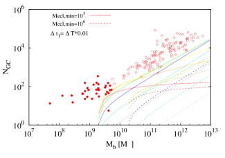
In Figure (10), we present a model for to match by setting to be with . It follows that dE galaxies are best represented by a model in which their GC population formed on a time scale with and . E galaxies require a similar short time for the formation of their GC population but and . Thus, the dE galaxies may have formed their GC population with a somewhat top-heavy ECMF, while massive star-bursting galaxies had an approximately Salpeter ECMF. However, this conclusion is not unique, because solution to the dE galaxies with are also possible by increasing the ratio .
4.2 SFR not equal over and
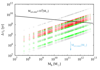
In the following we compute the initial or primordial value of the number of GCs as a function of galaxy mass. As shown in Figure (5), the SFRs need not be equal in the time (SFR1) and (SFR2). That is we assume SFR1 SFR2, but the SFR to be constant within time span and . By using equation (20) and the observational data (Figure 3) for , we can estimate . We set the minimum star cluster mass equal to , as Baumgardt & Makino (2003) suggested this as the minimum mass remaining bound as a cluster after 13 Gyr. We calculate the time scale for ranging between and and for different for clarity, we display only = 1.2, 1.9 and 2.5, see Figure (11). The solid black line indicates the star formation duration, , as defined by equation (9). Above this line, solutions become unphysical. increases with decreasing and the difference of the models for different increases with .
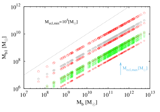
We calculate () and compare these results to . In Figure (12) we directly compare the total mass which forms in and the total mass of a galaxy. becomes unphysical above the dotted line, because larger than the total galaxy mass . As expected (total mass of stars formed during the GC formation epoch ) is smaller than (mass of galaxy).
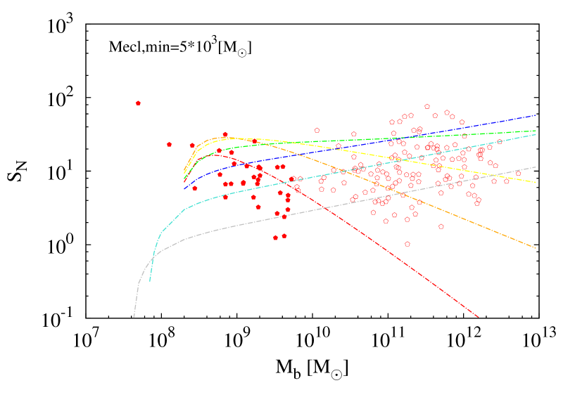
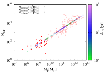
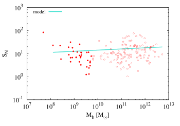
Weidner et al. (2004) suggested a star-cluster mass function population time scale of about yr. Using this and the galaxy formation time scale from downsizing (Recchi et al. 2009), we set between and yr. This is to obtain a physically realistic time scale for the formation of the GC system. By using equation (20), we obtain depending on and . In Figure (13) we compare the primordial and theoretical values of for and = 2.3 (since only equal to 2.3 can match for Branch I and II). Figure (13) indicates that increases with increasing , and yr represents most of the . The can be estimated using equation (17) after obtaining (Figure 14). This model is thus able to account for the observed variation of with for reasonable physical parameters.
5 Summary and conclusions
The specific frequency of GCs is a basic parameter to describe the GC system of a galaxy but remains poorly understood in the presently accepted galaxy formation framework (see also Kroupa 2015). The overall trend indicates high values of at opposite ends of the galaxy mass scale, while for a galaxy mass of around , becomes close to one. The idea developed here extends the notion raised by Mieske et al. (2014) to explain the ‘U’ -shaped relation between and through tidal erosion. The most important driver of the erosion process is a tidal field. We support this idea by showing the correlation between and (Figure 2). The GC survival fraction depends linearly on (), i.e., the observational data suggest that more GCs get destroyed in galaxies with a higher density which then have a smaller value of . It emerges that started approximately independently of galaxy mass, , but later changed to a ‘U’ -shape as a result of tidal erosion, which suggests that all early type galaxies had nearly the same efficiency to form young GCs. This in turn indicates that globular cluster formation is merely part of the universal star formation physics, which is evident in the solar neighborhood, and that it does not necessarily depend on the properties of the putative dark matter halos (see also Kroupa 2015).
The primordial number of clusters for the case is higher than that of , because the erosion rate of GCs depends on the degree of the radial velocity anisotropy of the GC system (Brockamp et al. 2014).
We constructed a model to explain the initial specific frequency of GCs in galaxies at constant SFR during different time scales and .
A model is suggested according to which a population of young clusters is formed following a cluster mass function which depends on the SFR. The theoretical specific frequency of the GC model explains the primordial value of , depending on the minimum star cluster mass and the slope of the cluster mass function. The models are reasonably well fit to for and . According to the models, we can infer that for a low SFR (low galaxy mass) we need a lower minimum cluster mass and smaller , while for a larger SFR (large galaxy masses) we need a higher minimum cluster mass.
For the model with shorter than , we can match the primordial for yr and = . The best explanation for dE galaxies is the model with = and = 2.3. The best model for E galaxies is for between and and between 1.5 and 2.5. The existence of this difference may indicate a different formation mechanism for dE and E galaxies, respectively (Okazaki & Taniguchi 2000; Dabringhausen & Kroupa 2013). We also see a possible hint that the embedded cluster mass function may become top-heavy (smaller ) in major galaxy-wide star burst, in support of the independent evidence found by Weidner et al. (2013)
Thus, by considering that all stars form in correlated star formation events (i.e. embedded clusters) it is naturally possible to account for the observed dependency of on galaxy mass . The large spread of values at a given and the difference of with for dE and E galaxies (Branch I and Branch II, respectively) suggest that the detailed star-formation events varied between these systems. But the overall can be understood in terms of the above assumption, that is, in terms of universal purely baryonic processes playing the same role in all systems.
Acknowledgments
We thank M. Kruckow, M. Brockamp, A. H. W. Küpper, M. Marks and A. Dieball for useful discussions and suggestions and Z. Randriamanakoto and C. Schulz for providing data. We used the publicly available data from W. E. Harris (http://physwww.mcmaster.ca/harris/Databases.html). R.A.G.L. acknowledges the financial support of DGAPA, UNAM (PASPA program and project IN108518).
References
- Ashman & Zepf (1992) Ashman, K. M. & Zepf, S. E. 1992, ApJ, 384, 50
- Baumgardt & Makino (2003) Baumgardt, H. & Makino, J. 2003, MNRAS, 340, 227
- Beasley et al. (2002) Beasley, M. A., Baugh, C. M., Forbes, D. A., Sharples, R. M., & Frenk, C. S. 2002, MNRAS, 333, 383
- Briceño et al. (2002) Briceño, C., Luhman, K. L., Hartmann, L., Stauffer, J. R., & Kirkpatrick, J. D. 2002, ApJ, 580, 317
- Brockamp et al. (2014) Brockamp, M., Küpper, A. H. W., Thies, I., Baumgardt, H., & Kroupa, P. 2014, MNRAS, 441, 150
- Brodie & Strader (2006) Brodie, J. P. & Strader, J. 2006, ARAA, 44, 193
- Bruzual & Charlot (2003) Bruzual, G. & Charlot, S. 2003, MNRAS, 344, 1000
- Chandar et al. (2004) Chandar, R., Whitmore, B., & Lee, M. G. 2004, ApJ, 611, 220
- Chandar et al. (2011) Chandar, R., Whitmore, B. C., Calzetti, D., Nino, D. D., Kennicutt, R. C., Regan, M., & Schinnerer, E. 2011, The Astrophysical Journal, 727, 88
- Dabringhausen et al. (2008) Dabringhausen, J., Hilker, M., & Kroupa, P. 2008, MNRAS, 386, 864
- Dabringhausen & Kroupa (2013) Dabringhausen, J. & Kroupa, P. 2013, MNRAS, 429, 1858
- Dekel & Birnboim (2006) Dekel, A. & Birnboim, Y. 2006, MNRAS, 368, 2
- Egusa et al. (2009) Egusa, F., Kohno, K., Sofue, Y., Nakanishi, H., & Komugi, S. 2009, ApJ, 697, 1870
- Egusa et al. (2004) Egusa, F., Sofue, Y., & Nakanishi, H. 2004, PASJ, 56, L45
- Elmegreen & Efremov (1997) Elmegreen, B. G. & Efremov, Y. N. 1997, ApJ, 480, 235
- Forbes et al. (1997) Forbes, D. A., Brodie, J. P., & Grillmair, C. J. 1997, AJ, 113, 1652
- Forte et al. (1982) Forte, J. C., Martinez, R. E., & Muzzio, J. C. 1982, AJ, 87, 1465
- Fukui & Kawamura (2010) Fukui, Y. & Kawamura, A. 2010, ARAA, 48, 547
- Georgiev et al. (2010) Georgiev, I. Y., Puzia, T. H., Goudfrooij, P., & Hilker, M. 2010, MNRAS, 406, 1967
- Goudfrooij et al. (2003) Goudfrooij, P., Strader, J., Brenneman, L., Kissler-Patig, M., Minniti, D., & Edwin Huizinga, J. 2003, MNRAS, 343, 665
- Gratton et al. (2003) Gratton, R. G., Bragaglia, A., Carretta, E., Clementini, G., Desidera, S., Grundahl, F., & Lucatello, S. 2003, A&A, 408, 529
- Graves & Faber (2010) Graves, G. J. & Faber, S. M. 2010, ApJ, 717, 803
- Harris (1991) Harris, W. E. 1991, ARAA, 29, 543
- Harris et al. (2013) Harris, W. E., Harris, G. L. H., & Alessi, M. 2013, ApJ, 772, 82
- Harris & van den Bergh (1981) Harris, W. E. & van den Bergh, S. 1981, AJ, 86, 1627
- Kroupa (2005) Kroupa, P. 2005, in ESA Special Publication, Vol. 576, The Three-Dimensional Universe with Gaia, ed. C. Turon, K. S. O’Flaherty, & M. A. C. Perryman, 629
- Kroupa (2015) Kroupa, P. 2015, Canadian Journal of Physics, 93, 169
- Kroupa & Bouvier (2003) Kroupa, P. & Bouvier, J. 2003, MNRAS, 346, 369
- Kroupa & Weidner (2003) Kroupa, P. & Weidner, C. 2003, ApJ, 598, 1076
- Lada & Lada (2003) Lada, C. J. & Lada, E. A. 2003, ARAA, 41, 57
- Lamers et al. (2017) Lamers, H. J. G. L. M., Kruijssen, J. M. D., Bastian, N., Rejkuba, M., Hilker, M., & Kissler-Patig, M. 2017, A&A, 606, A85
- Larsen (2002) Larsen, S. S. 2002, AJ, 124, 1393
- Larsen & Richtler (2000) Larsen, S. S. & Richtler, T. 2000, A&A, 354, 836
- Megeath et al. (2016) Megeath, S. T., Gutermuth, R., Muzerolle, J., Kryukova, E., Hora, J. L., Allen, L. E., Flaherty, K., Hartmann, L., Myers, P. C., Pipher, J. L., Stauffer, J., Young, E. T., & Fazio, G. G. 2016, AJ, 151, 5
- Meidt et al. (2015) Meidt, S. E., Hughes, A., Dobbs, C. L., Pety, J., Thompson, T. A., García-Burillo, S., Leroy, A. K., Schinnerer, E., Colombo, D., Querejeta, M., Kramer, C., Schuster, K. F., & Dumas, G. 2015, ApJ, 806, 72
- Mieske et al. (2014) Mieske, S., Küpper, A. H. W., & Brockamp, M. 2014, A&A, 565, L6
- Miller & Lotz (2007) Miller, B. W. & Lotz, J. M. 2007, ApJ, 670, 1074
- Miller et al. (1998) Miller, B. W., Lotz, J. M., Ferguson, H. C., Stiavelli, M., & Whitmore, B. C. 1998, ApJL, 508, L133
- Neilsen et al. (1997) Neilsen, Jr., E. H., Tsvetanov, Z. I., & Ford, H. C. 1997, ApJ, 483, 745
- Okazaki & Taniguchi (2000) Okazaki, T. & Taniguchi, Y. 2000, ApJ, 543, 149
- Peng et al. (2008) Peng, E. W., Jordán, A., Côté, P., Takamiya, M., West, M. J., Blakeslee, J. P., Chen, C.-W., Ferrarese, L., Mei, S., Tonry, J. L., & West, A. A. 2008, ApJ, 681, 197
- Randriamanakoto et al. (2013) Randriamanakoto, Z., Escala, A., Väisänen, P., Kankare, E., Kotilainen, J., Mattila, S., & Ryder, S. 2013, ApJL, 775, L38
- Recchi et al. (2009) Recchi, S., Calura, F., & Kroupa, P. 2009, A&A, 499, 711
- Rhode et al. (2007) Rhode, K. L., Zepf, S. E., Kundu, A., & Larner, A. N. 2007, AJ, 134, 1403
- Schulz et al. (2015) Schulz, C., Pflamm-Altenburg, J., & Kroupa, P. 2015, A&A, 2015.
- Schweizer (1987) Schweizer, F. 1987, in Nearly Normal Galaxies. From the Planck Time to the Present, ed. S. M. Faber, 18–25
- Smith & Lucey (2013) Smith, R. J. & Lucey, J. R. 2013, MNRAS, 434, 1964
- Thomas et al. (1999) Thomas, D., Greggio, L., & Bender, R. 1999, MNRAS, 302, 537
- Tiret et al. (2011) Tiret, O., Salucci, P., Bernardi, M., Maraston, C., & Pforr, J. 2011, MNRAS, 411, 1435
- Weidner & Kroupa (2004) Weidner, C. & Kroupa, P. 2004, MNRAS, 348, 187
- Weidner et al. (2004) Weidner, C., Kroupa, P., & Larsen, S. S. 2004, MNRAS, 350, 1503
- Weidner et al. (2013) Weidner, C., Kroupa, P., Pflamm-Altenburg, J., & Vazdekis, A. 2013, MNRAS, 436, 3309
- Whitmore et al. (2010) Whitmore, B. C., Chandar, R., Schweizer, F., Rothberg, B., Leitherer, C., Rieke, M., Rieke, G., Blair, W. P., Mengel, S., & Alonso-Herrero, A. 2010, AJ, 140, 75
- Wu & Kroupa (2013) Wu, X. & Kroupa, P. 2013, MNRAS, 435, 1536