Knowing The What But Not The Where in Bayesian Optimization

Abstract

Bayesian optimization has demonstrated impressive success in finding the optimum input $\mathbf{x}^{*}$ and output $f^{*}=f(\mathbf{x}^{*})=\max f(\mathbf{x})$ of a black-box function $f$. In some applications, however, the optimum output $f^{*}$ is known in advance and the goal is to find the corresponding optimum input $\mathbf{x}^{*}$. In this paper, we consider a new setting in BO in which the knowledge of the optimum output $f^{*}$ is available. Our goal is to exploit the knowledge about $f^{*}$ to search for the input $\mathbf{x}^{*}$ efficiently. To achieve this goal, we first transform the Gaussian process surrogate using the information about the optimum output. Then, we propose two acquisition functions, called confidence bound minimization and expected regret minimization. We show that our approaches work intuitively and give quantitatively better performance against standard BO methods. We demonstrate real applications in tuning a deep reinforcement learning algorithm on the CartPole problem and XGBoost on Skin Segmentation dataset in which the optimum values are publicly available.

1 Introduction

Bayesian optimization (BO) (Brochu et al., 2010; Shahriari et al., 2016; Oh et al., 2018; Ru et al., 2020) is an efficient method for the global optimization of a black-box function. BO has been successfully employed in selecting chemical compounds (Hernández-Lobato et al., 2017), material design (Frazier & Wang, 2016; Li et al., 2018), algorithmic assurance (Gopakumar et al., 2018), and in search for hyperparameters of machine learning algorithms (Snoek et al., 2012; Klein et al., 2017; Chen et al., 2018). These recent results suggest BO is more efficient than manual, random, or grid search.

Bayesian optimization finds the global maximizer $\mathbf{x}^{*}=\arg\max_{\mathbf{x}\in\mathcal{X}}f(\mathbf{x})$ of the black-box function $f$ by incorporating prior beliefs about $f$ and updating the prior with evaluations where $\mathcal{X}\subset\mathcal{\mathbb{R}}^{d}$ is the search domain. The model used for approximating the black-box function is called the surrogate model. A popular choice for a surrogate model is the Gaussian process (GP) (Rasmussen, 2006) although there are existing alternative options, such as random forests (Hutter et al., 2011), deep neural networks (Snoek et al., 2015), Bayesian neural networks (Springenberg et al., 2016) and Mondrian trees (Wang et al., 2018). This surrogate model is then used to define an acquisition function which determines the next query of the black-box function.

In some settings, the optimum output $f^{*}=f(\mathbf{x}^{*})$ is known in advance. For example, the optimal reward is available for common reinforcement learning benchmarks or we know the optimum accuracy is $100$ in tuning classification algorithm for specific datasets. As another example in inverse optimization, we retrieve the input resulting the given target (Ahuja & Orlin, 2001; Perdikaris & Karniadakis, 2016). The question is how to efficiently utilize such prior knowledge to find the optimal inputs using the fewest number of queries.

In this paper, we give the first BO approach to this setting in which we know what we are looking for, but we do not know where it is. Specifically, we know the optimum output $f^{*}=\max_{\mathbf{x}\in\mathcal{X}}f(\mathbf{x})$ and aim to search for the unknown optimum input $\mathbf{x}^{*}=\arg\max_{\mathbf{x}\in\mathcal{X}}f(\mathbf{x})$ by utilizing $f^{*}$ value.

We incorporate the information about $f^{*}$ into Bayesian optimization in the following ways. First, we use the knowledge of $f^{*}$ to build a transformed GP surrogate model. Our intuition in transforming a GP is based on the fact that the black-box function value $f(\mathbf{x})$ should not be above the threshold $f^{*}$ (since $f^{*}\geq f(\mathbf{x}),\forall\mathbf{x}\in\mathcal{X}$, by definition). As a result, the GP surrogate should also follow this property. Second, we propose two acquisition functions which make decisions informed by the $f^{*}$ value, namely confidence bound minimization and expected regret minimization.

We validate our model using benchmark functions and tuning a deep reinforcement learning algorithm where we observe the optimum value in advance. These experiments demonstrate that our proposed framework works both intuitively better and experimentally outperforms the baselines. Our main contributions are summarized as follows:

• a first study of Bayesian optimization for exploiting the known optimum output $f^{*}$;

• a transformed Gaussian process surrogate using the knowledge of $f^{*}$; and

• two novel acquisition functions to efficiently select the optimum location given $f^{*}$.

2 Preliminaries

In this section, we review some of the existing acquisition functions from the Bayesian optimization literature which can readily incorporate the known $f^{*}$ value. Then, we summarize the possible transformation techniques used to control the Gaussian process using $f^{*}$.

2.1 Available acquisition functions for the known $f^{*}$

Bayesian optimization uses an acquisition function to make a query. Among many existing acquisition functions (Hennig & Schuler, 2012; Hernández-Lobato et al., 2014; Wang et al., 2016; Letham et al., 2019; Astudillo & Frazier, 2019; Nguyen et al., 2019), we review two acquisition functions which can incorporate the known optimum output $f^{*}$ directly in their forms. We then use the two acquisition functions as the baselines for comparison.

Expected improvement with known incumbent $f^{*}$.

EI (Mockus et al., 1978) considers the expectation over the improvement function which is defined over the incumbent $\xi$ as $\mathbb{E}\left[I_{t}\left(\mathbf{x}\right)\right]=\mathbb{E}\left[\max\left\{0,f\left(\mathbf{x}\right)-\xi\right\}\right]$. One needs to define the incumbent to improve upon. Existing research has considered modifying this incumbent with various choices (Wang & de Freitas, 2014; Berk et al., 2018). The typical choice of the incumbent is the best observed value so far in the observation set $\xi=\max_{y_{i}\in\mathcal{D}_{t-1}}y_{i}$ where $\mathcal{D}_{t-1}$ is the dataset upto iteration $t$. Given the known optimum output $f^{*}$, one can readily use it as the incumbent, i.e., setting $\xi=f^{*}$ to have the following forms:

$$\alpha^{\textrm{EI}^{*}}\left(\mathbf{x}\right) =\sigma\left(\mathbf{x}\right)\phi\left(z\right)+\left[\mu\left(\mathbf{x}\right)-f^{*}\right]\Phi\left(z\right)$$ (1)

where $\mu(\mathbf{x})$ is the GP predictive mean, $\sigma(\mathbf{x})$ is the GP predictive variance, $z=\frac{\mu\left(\mathbf{x}\right)-f^{*}}{\sigma\left(\mathbf{x}\right)}$, $\phi$ is the standard normal p.d.f. and $\Phi$ is the c.d.f.

Output entropy search with known $f^{*}$.

The second group of acquisition functions, which are readily to incorporate the known optimum, include several approaches gaining information about the output, such as output-space PES (Hoffman & Ghahramani, 2015), MES (Wang & Jegelka, 2017) and FITBO (Ru et al., 2018). These approaches consider different ways to gain information about the optimum output $f^{*}$. When $f^{*}$ is not known in advance, Hoffman & Ghahramani (2015); Wang & Jegelka (2017) utilize Thompson sampling to sample $f^{*}$, or a collection of $f_{m}^{*},\forall m\leq M$, while Ru et al. (2018) consider $f^{*}$ as a hyperparameter. After generating optimum value samples, the above approaches consider different approximation strategies.

Since the optimum output $f^{*}$ is available in our setting, we can use it directly within the above approaches. We select to review the MES due to its simplicity and closed-form computation. Given the known $f^{*}$ value, MES approximates $I(\mathbf{x},y;f^{*})$ using a truncated Gaussian distribution such that the distribution of $y$ needs to satisfy $y<f^{*}$, to obtain,

$$I(\mathbf{x},y;f^{*}) =H\left[p(y|D_{t},\mathbf{x})\right]-\mathbb{E}[H\left(p(y|D_{t},\mathbf{x},f^{*})\right)]{p(f^{*}|D_{t})}.$$

Let $\gamma(\mathbf{x},f^{*})=\frac{f^{*}-\mu(\mathbf{x})}{\sigma(\mathbf{x})}$, we have the MES^∗ as

$$\alpha^{\textrm{MES}{}^{*}}(\mathbf{x}\mid f^{*})= \frac{\gamma(\mathbf{x},f^{*})\phi\left[\gamma(\mathbf{x},f^{*})\right]}{2\Phi\left[\gamma(\mathbf{x},f^{*})\right]}-\log\Phi\left[\gamma(\mathbf{x},f^{*})\right].$$

2.2 Gaussian process transformation for $f\leq f^{*}$

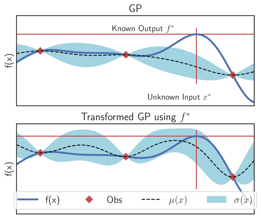
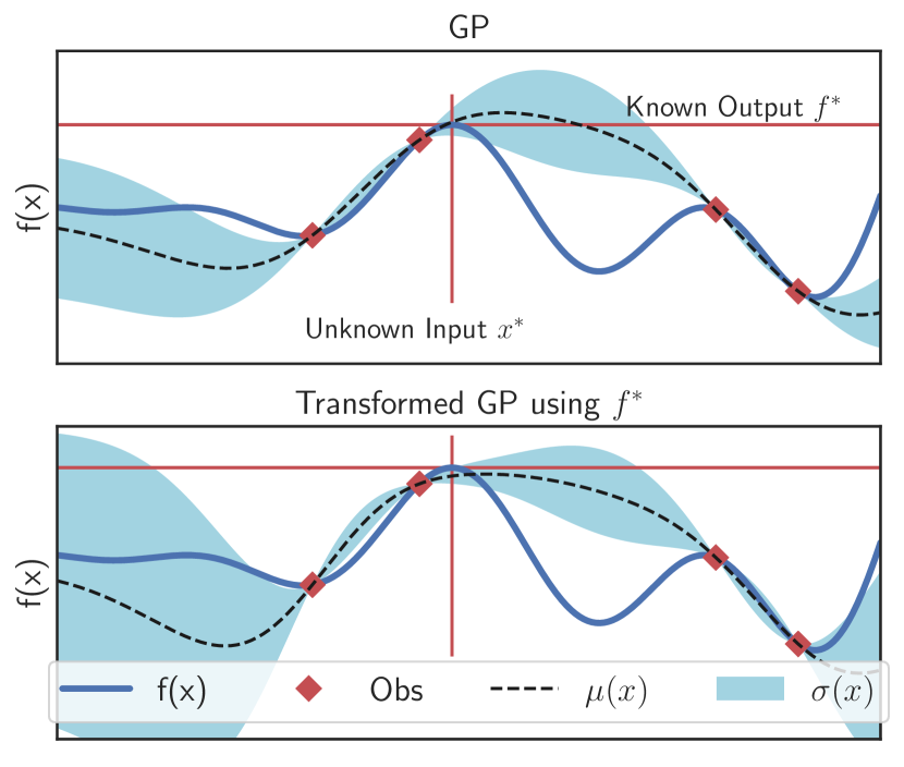
Figure 1: Comparison of the transformed GP with the GP using two different functions in left and right. The known $f^{*}$ output and unknown input $\mathbf{x}^{*}$ are highlighted by horizontal and vertical red lines respectively. Top: the GP allows $\mu(\mathbf{x})$ to go above and below $f^{*}$. Bottom: the transformed GP will lift up the surrogate model closer to the known optimum output $f^{*}$ (left) and not go above $f^{*}$ (right).

We summarize several transformation approaches which can be potentially used to enforce that the function $f$ is everywhere below $f^{*}$, given the upper bound $f^{*}=\max_{\forall\mathbf{x}}f(\mathbf{x})$.

The first category is to use functions such as sigmoid and tanh. However, there are two problems with such functions. The first problem is that they both require the knowledge of the lower bound, $\min f(\mathbf{x})$, and the upper bound, $\max f(\mathbf{x})$, for the normalization to the predefined ranges, i.e. $[0,1]$ for sigmoid and $[-1,1]$ for tanh. However, we do not know the lower bound in our setting. The second problem is that exact inference for a GP is analytically intractable under these transformations. Particularly, this will become the Gaussian process classification problem (Nickisch & Rasmussen, 2008) where approximation must be made, such as using expectation propagation (Kuss & Rasmussen, 2005; Riihimäki et al., 2013; Hernández-Lobato & Hernández-Lobato, 2016).

The second category is to transform the output of a GP using warping (MacKay, 1998; Snelson et al., 2004). However, the warped GP is less efficient in the context of Bayesian optimization. This is because a warped GP requires more data points to learn the mapping from original to transformed space while we only have a small number of observations in BO setting.

The third category makes use of a linearization trick (Osborne et al., 2012; Gunter et al., 2014) as GPs are closed under linear transformations. This linearization ensures that we arrive at another GP after transformation given our existing GP. In this paper, we shall follow this linearization trick to transform the surrogate model given $f^{*}$.

3 Bayesian Optimization When The True Optimum Output Is Known

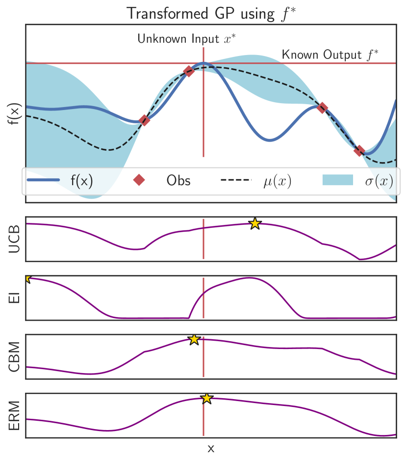
Figure 2: Illustration of the proposed acquisition functions CBM and ERM. A yellow star indicates the maximum of the acquisition function and thus is the selected point. Using the knowledge of $f^{*}$, CBM and ERM can better identify $\mathbf{x}^{*}$ while EI and UCB cannot.

We present a new approach for Bayesian optimization given situations where the knowledge of optimum output (value) $f^{*}=\max_{\mathbf{x}\in\mathcal{X}}f(\mathbf{x})$ is available. Our goal is to utilize this knowledge to improve BO performance in finding the unknown optimum input (location) $\mathbf{x}^{*}=\arg\max_{\mathbf{x}\in\mathcal{X}}f(\mathbf{x})$. We first encode $f^{*}$ to build an informed GP surrogate model through transformation and then we propose two acquisition functions which effectively exploit knowledge of $f^{*}$.

3.1 Transformed Gaussian process

We make use of the knowledge about the optimum output to control the GP surrogate model through transformation. Our transformation starts with two key observations that firstly the function value $f(\mathbf{x})$ should reach the optimum output; but secondly never be greater than the optimal value $f^{*}$, by definition of $f^{*}$ being a maximum value. Therefore, the desired GP surrogate should not go above this threshold. Based on this intuition, we propose the GP transformation given $f^{*}$ as follows

$$f(\mathbf{x}) =f^{*}-\frac{1}{2}g^{2}(\mathbf{x})$$

$$g(\mathbf{x}) \sim GP(m_{0},K).$$

Our above transformation avoids the potential issues described in Sec. 2.2. That is we don’t need a lot of samples to learn the transformation mapping for the desired property that the function is always held $f^{*}\geq f(\mathbf{x}),\forall\mathbf{x}\in\mathcal{X}$ as $g^{2}(\mathbf{x})\geq 0$. The prior mean for $g(\mathbf{x})$ can be used either $m_{0}=0$ or $m_{0}=\sqrt{2f^{*}}$. These choices will bring two different effects. A zero mean prior $m_{0}=0$ will tend to lift up the surrogate model closer to $f^{*}$ as $f(\mathbf{x})=f^{*}$ when $g(\mathbf{x})=0$. On the other hand, non-zero mean $m_{0}=\sqrt{2f^{*}}$ will encourage the mean prior of $f$ closer to zero – as a common practice in GP modeling where the output is standardized around zero $y\sim\mathcal{N}(0,1)$.

Given the observations $\mathcal{D}_{f}=(\mathbf{x}_{i},y_{i})_{i=1}^{N}$, we can compute the observations for $g$, i.e., $\mathcal{D}_{g}=(\mathbf{x}_{i},g_{i})_{i=1}^{N}$ where $g_{i}=\sqrt{2(f^{*}-y_{i})}$. Then, we can write the posterior of $p\left(g\mid\mathcal{D}_{g},f^{*}\right)\sim\mathcal{N}\left(\mu_{g}(\mathbf{x}),\sigma_{g}(\mathbf{x})\right)$ as $\mu_{g}(\mathbf{x})=m_{0}+\mathbf{k}_{*}\mathbf{K}^{-1}\left(\mathbf{g}-m_{0}\right)$ and $\sigma_{g}^{2}\left(\mathbf{x}\right)=k_{**}-\mathbf{k}_{*}\mathbf{K}^{-1}\mathbf{k}_{*}^{T}$ where $m_{0}$ is the prior mean of $g(\mathbf{x})$.

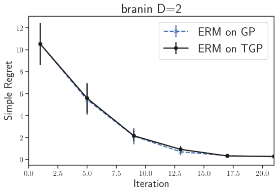
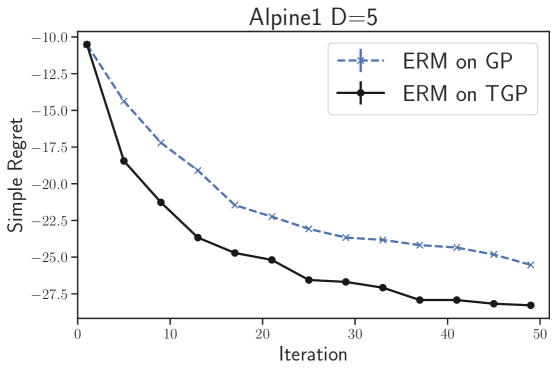
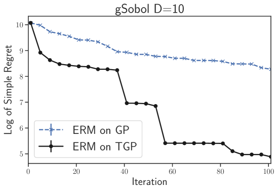
Figure 3: We show that our model performs much better using transformed Gaussian process (TGP) than the vanilla GP. The knowledge of $f^{*}$ is useful to inform the surrogate model for better optimization, especially in high dimensional functions.

We don’t introduce any extra parameter for the above transformation. However, the transformation causes the distribution for any $f$ to become a non-central $\chi^{2}$ process, making the analysis intractable. To tackle this problem and obtain a posterior distribution $p\left(f\mid\mathcal{D}_{f},f^{*}\right)$ that is also Gaussian, we employ an approximation technique presented in Gunter et al. (2014); Ru et al. (2018). That is, we perform a local linearization of the transformation $h(g)=f^{*}-\frac{1}{2}g^{2}(\mathbf{x})$ around $g_{0}$ and obtain $f\approx h\left(g_{0}\right)+h^{\prime}\left(g_{0}\right)\left(g-g_{0}\right)$ where the gradient $h^{\prime}(g_{0})=-g$. Following Gunter et al. (2014); Ru et al. (2018), we set $g_{0}=\mu_{g}$ to the mode of the posterior distribution $p\left(g\mid.\right)$ and obtain an expression for $f$ as

$$f(\mathbf{x}) \approx f^{*}-\frac{1}{2}\mu_{g}^{2}(\mathbf{x})-\mu_{g}(\mathbf{x})\left[g(\mathbf{x})\text{\textminus}\mu_{g}(\mathbf{x})\right]$$

$$=f^{*}+\frac{1}{2}\mu_{g}^{2}(\mathbf{x})-\mu_{g}(\mathbf{x})g(\mathbf{x}).$$

We have considered the mode $g_{0}$ of linear approximation to be the multivariate function $\mu_{g}(\mathbf{x}),\forall\mathbf{x}$. As the property of Taylor expansion, the approximation is very good at the mode $g_{0}$ and thus $\mu_{g}$. Since the linear transformation of a Gaussian process remains Gaussian, the predictive posterior distribution for $f$ now has a closed form for $p\left(f\mid.\right)=\mathcal{N}\left(f\mid\mu,\sigma\right)$ where the predictive mean and variance are given by

$$\mu(\mathbf{x}) =f^{*}-\frac{1}{2}\mu_{g}^{2}(\mathbf{x}),$$ (2)

$$\sigma(\mathbf{x}) =\mu_{g}(\mathbf{x})\sigma_{g}(\mathbf{x})\mu_{g}(\mathbf{x}).$$ (3)

These Eqs. (2) and (3) are the key to compute our acquisition functions in the next sections. As the effect of transformation, the predictive uncertainty $\sigma(\mathbf{x})$ of the transformed GP becomes larger than in the case of vanilla GP at the location where $\mu(\mathbf{x})$ is low. This is because $\mu_{g}(\mathbf{x})$ is high when $\mu(\mathbf{x})$ is low and thus $\sigma(\mathbf{x})$ is high in Eq. (3). This property may let other acquisition functions (e.g., UCB, EI) explore more aggressively than they should. We further examine these effects in the supplement.

We visualize the property of our transformed GP and compare with the vanilla GP in Fig. 1. By transforming the GP using $f^{*}$, we encode the knowledge about $f^{*}$ into the surrogate model, and thus are able to enforce that the surrogate model gets close to but never above $f^{*}$, as desired, unlike the vanilla GP. In the supplement, we provide further illustration that transforming the surrogate model can help to find the optimum faster. We present quantitative comparison of our transformed GP and vanilla GP in Fig. 3 and in the supplement.

3.2 Confidence bound minimization

In this section, we introduce confidence bound minimization (CBM) to efficiently select the (unknown) optimum location $\mathbf{x}^{*}$ given $f^{*}=f(\mathbf{x}^{*})$. Our idea is based on the underlying concept of GP-UCB (Srinivas et al., 2010). We consider the GP surrogate at any location $\mathbf{x}\in\mathcal{X}$ w.h.p.

$$\mu(\mathbf{x})-\sqrt{\beta_{t}}\sigma(\mathbf{x}) \leq f(\mathbf{x})\leq\mu(\mathbf{x})+\sqrt{\beta_{t}}\sigma(\mathbf{x})$$ (4)

where $\beta_{t}$ is a hyperparameter. Given the knowledge of $f^{*}$, we can express this property at the optimum location $\mathbf{x}^{*}$ where $f^{*}=f(\mathbf{x}^{*})$ to have w.h.p.

$$\mu(\mathbf{x}^{*})-\sqrt{\beta_{t}}\sigma(\mathbf{x}^{*}) \leq f^{*}\leq\mu(\mathbf{x}^{*})+\sqrt{\beta_{t}}\sigma(\mathbf{x}^{*}).$$

This is equivalent to write $|\mu(\mathbf{x}^{*})-f^{*}|\leq\sqrt{\beta_{t}}\sigma(\mathbf{x}^{*})$. Therefore, we can find the next point $\mathbf{x}_{t}$ by balancing the posterior mean being close to the known optimum $f^{*}$ with having low variance. That is

$$\alpha_{t}^{\textrm{CBM}}(\mathbf{x}) =|\mu(\mathbf{x})-f^{*}|+\sqrt{\beta_{t}}\sigma(\mathbf{x})$$

where $\mu(\mathbf{x})$ and $\sigma(\mathbf{x})$ are the GP mean and variance from Eq. (2) and Eq. (3) respectively. We select the next point by taking

$$\mathbf{x}_{t+1}= \underset{{}_{\mathbf{x}\in\mathcal{X}}}{\text{argmin}\ }\alpha_{t}^{\textrm{CBM}}(\mathbf{x}).$$ (5)

In the above objective function, we aim to quickly locate the area potentially containing an optimum. Since the acquisition function is non-negative, $\alpha^{\textrm{CBM}}(\mathbf{x})\geq 0,\forall\mathbf{x}\in\mathcal{X}$, it takes the minimum value at the ideal location where $\mu(\mathbf{x}_{t})=f^{*}$ and $\sigma(\mathbf{x}_{t})=0$. When these two conditions are met, we can conclude that $f(\mathbf{x}_{t})=f(\mathbf{x}^{*})$ and thus $\mathbf{x}_{t}$ is what we are looking for, as the property of Eq. (4).

Because the CBM involves a hyperparameter $\beta$ to which performance can be sensitive, we below propose another acquisition function incorporating the knowledge of $f^{*}$ using no hyperparameter.

3.3 Expected regret minimization

We next develop our second acquisition function using $f^{*}$, called expected regret minimization (ERM). We start with the regret function $r\left(\mathbf{x}\right)=f^{*}-f(\mathbf{x})$. The probability of regret $r\left(\mathbf{x}\right)$ on a normal posterior distribution is as follows

$$p\left(r\right)= \frac{1}{\sqrt{2\pi}\sigma\left(\mathbf{x}\right)}\exp\left(-\frac{1}{2}\frac{\left[f^{*}-\mu\left(\mathbf{x}\right)-r(\mathbf{x})\right]^{2}}{\sigma^{2}\left(\mathbf{x}\right)}\right).$$ (6)

As the end goal in optimization is to minimize the regret, we consider our acquisition function to minimize this expected regret as $\alpha^{\textrm{ERM}}\left(\mathbf{x}\right)=\mathbb{E}\left[r\left(\mathbf{x}\right)\right]$. Using the likelihood function in Eq. (9), we write the expected regret minimization acquisition function as

$$\mathbb{E}\left[r\left(\mathbf{x}\right)\right]= \int\frac{r}{\sqrt{2\pi}\sigma\left(\mathbf{x}\right)}\exp\left(-\frac{1}{2}\frac{\left[f^{*}-\mu\left(\mathbf{x}\right)-r(\mathbf{x})\right]^{2}}{\sigma^{2}\left(\mathbf{x}\right)}\right)dr.$$

Let $z=\frac{f^{*}-\mu\left(\mathbf{x}\right)}{\sigma\left(\mathbf{x}\right)}$, we obtain the closed-form computation as

$$\alpha^{\textrm{ERM}}\left(\mathbf{x}\right) =\sigma\left(\mathbf{x}\right)\phi\left(z\right)+\left[f^{*}-\mu\left(\mathbf{x}\right)\right]\Phi\left(z\right)$$ (7)

where $\phi\left(z\right)$ and $\Phi\left(z\right)$ are the standard normal p.d.f. and c.d.f., respectively. To select the next point, we minimize this acquisition function which is equivalent to minimizing the expected regret,

$$\mathbf{x}_{t+1} =\arg\min_{\mathbf{x}\in\mathcal{X}}\alpha^{\textrm{ERM}}\left(\mathbf{x}\right)=\arg\min_{\mathbf{x}\in\mathcal{X}}\mathbb{E}\left[r\left(\mathbf{x}\right)\right].$$ (8)

Our choice in Eq. (8) is where to minimize the expected regret. We can see that this acquisition function is always positive $\alpha^{\textrm{ERM}}(\mathbf{x})\geq 0,\forall\mathbf{x}\in\mathcal{X}$. It is minimized at the ideal location $\mathbf{x}_{t}$, i.e., $\alpha^{\textrm{ERM}}(\mathbf{x}_{t})=\mathbb{E}\left[r\left(\mathbf{x}\right)\right]=0$, when $f^{*}-\mu(\mathbf{x}_{t})=0$ and $\sigma(\mathbf{x}_{t})=0$. This case happens at the desired location where the GP predictive value is equal to the true $f^{*}$ with zero GP uncertainty.

Algorithm 1 BO with known optimum output.

  Input: #iter $T$, optimum value $f^{*}=\max_{\mathbf{x}\in\mathcal{X}}f(\mathbf{x})$

1:  while  $t\leq T$ and $f^{*}>\max_{\forall y_{i}\in D_{t}}y_{i}$  do

2:     Construct a transformed Gaussian process surrogate model from $\mathcal{D}_{t}$ and $f^{*}$.

3:     Estimating $\mu$ and $\sigma$ from Eqs. (2) and (3).

4:     Select $\mathbf{x}_{t}=\arg\min_{\mathbf{x}\in\mathcal{X}}\alpha_{t}^{\textrm{ERM}}(\mathbf{x})$, or $\alpha_{t}^{\textrm{CBM}}(\mathbf{x})$, using the above transformed GP model.

5:     Evaluate $y_{t}=f\left(\mathbf{x}_{t}\right)$, set $g_{t}=\sqrt{2(f^{*}-y_{t})}$ and augment $\mathcal{D}_{t}=\mathcal{D}_{t-1}\cup\left(\mathbf{x}_{t},y_{t},g_{t}\right)$.

6:  end while

Although our ERM is inspired by the EI in the way that we define the regret function and take the expectation, the resulting approach is different in the following. The original EI strategy is to balance exploration and exploitation, i.e., prefers high GP mean and high GP variance. On the other hand, ERM will not encourage such trade-off directly. Instead, ERM selects the point to minimize the expected regret $\mathbb{E}\left[f^{*}-f(\mathbf{x})\right]$ with $\mu(\mathbf{x})$ being closer to the known $f^{*}$ while having low variance to make sure that the GP estimation at our chosen location is correct. Then, if the chosen location turns out to be not expected (e.g., poor function value), the GP is updated and ERM will move to another place which minimizes the new expected regret. Therefore, these behaviors of EI and our ERM are radically different.

Algorithm.

We summarize all steps in Algorithm 1. Given the original observation $\left\{\mathbf{x}_{i},y_{i}\right\}_{i=1}^{N}$ and $f^{*}$, we compute $g_{i}=\sqrt{2(f^{*}-y_{i})}$, then build a transformed GP using $\{\mathbf{x}_{i},g_{i}\}_{i=1}^{N}$. Using a transformed GP, we can predict the mean $\mu(\mathbf{x})$ and uncertainty $\sigma(\mathbf{x})$ at any location $\mathbf{x}$ from Eqs. (2) and (3) which are used to compute the CBM and ERM acquisition functions in Eq. (5) and Eq. (8). Our formulas are in closed-forms and the algorithm is easy to implement. In addition, our computational complexity is as cheap as the GP-UCB and EI.

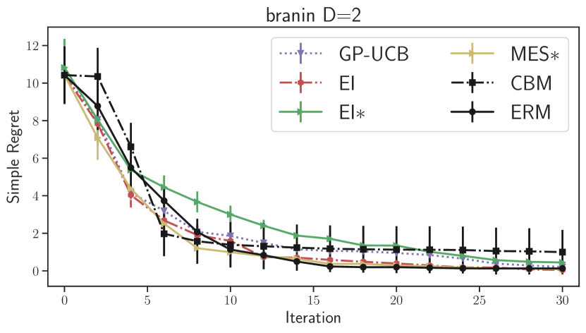
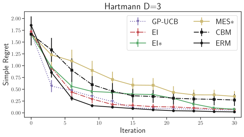
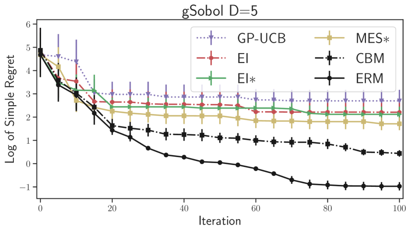
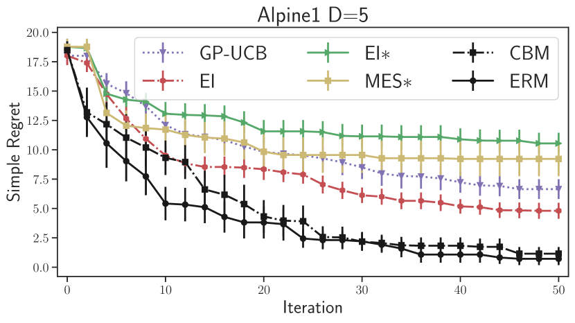
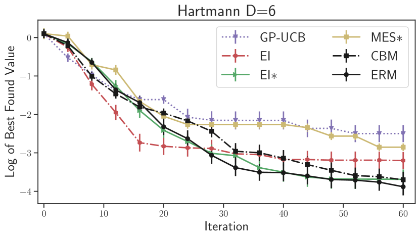
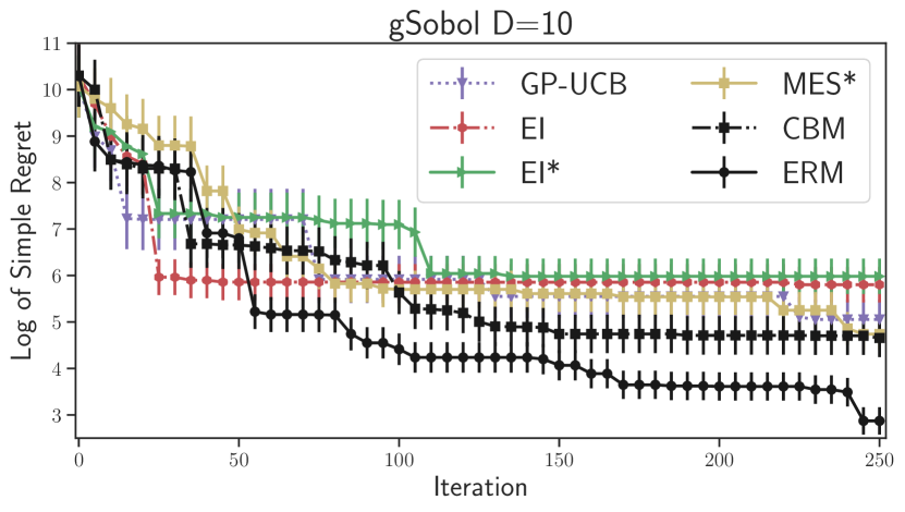
Figure 4: Optimization comparison using benchmark functions from $D=2$ to $D=10$ dimensions. We demonstrate that the known optimum output $f^{*}$ will significantly boost the performances in high dimensions, such as in Alpine1 $D=5$, gSobol $D=5$ and $D=10$.

Illustration of CBM and ERM

We illustrate in Fig. 2 our proposed CBM and ERM comparing to the standard UCB and EI with both vanilla GP and transformed GP settings. Our acquisition functions make use of the knowledge about $f^{*}$ to make an informed decision about where we should query. That is, CBM and ERM will select the location where the GP mean $\mu(\mathbf{x})$ is close to the optimal value $f^{*}$ and we are highly certain about it – or low $\sigma(\mathbf{x})$. On the other hand, GP-UCB and EI will always keep exploring as the principle of explore-exploit without using the knowledge of $f^{*}$. As the results, GP-UCB and EI can not identify the unknown location $\mathbf{x}^{*}$ efficiently as opposed to our acquisition functions.

4 Experiments

The main goal of our experiments is to show that we can effectively exploit the known optimum output to improve Bayesian optimization performance. We first demonstrate the efficiency of our model on benchmark functions. Then, we perform hyperparameter optimization for a XGBoost classification on Skin Segmentation dataset and a deep reinforcement learning task on CartPole problem where the optimum values are publicly available. We provide additional experiments in the supplement and the code is released at.

Settings.

All implementations are in Python. The experiments are independently performed $20$ times. We use the squared exponential kernel $k\left(x,x^{\prime}\right)=\exp\left(-||x-x^{\prime}||^{2}/\sigma_{l}\right)$ where $\sigma_{l}$ is optimized from the GP marginal likelihood, the input is scaled $x\sim\left[0,1\right]^{d}$ and the output is standardized $y\sim\mathcal{N}\left(0,1\right)$ for robustness. We follow Theorem 3 in Srinivas et al. (2010) to specify $\beta_{t}=2f^{*}+300\log^{3}(t/\delta)$.

To avoid our algorithms from the early exploitation, we use a standard BO (with GP and EI) at the earlier iterations and our proposed algorithms at later iterations once the $f^{*}$ value has been reached by the upper confidence bound. The reaching $f^{*}$ condition can be checked in each BO iteration using a global optimization toolbox, i.e., $\exists\mathbf{x}\mid f^{*}\leq\mu(\mathbf{x})+\sqrt{\beta_{t}}\sigma(\mathbf{x})$.

Our CBM and ERM use a transformed Gaussian process (Sec. 3.1) in all experiments. We learn empirically that using a transformed GP as a surrogate will boost the performance for our CBM and ERM significantly against the case of using vanilla GP. For other baselines, we use both surrogates and report the best performance. We present further details of experiments in the supplement.

Baselines.

To the best of our knowledge, there is no baseline in directly using the known optimum output for BO. We select to compare our model with the vanilla BO without knowing the optimum value including the GP-UCB (Srinivas et al., 2010) and EI (Mockus et al., 1978). In addition, we use two other baselines using $f^{*}$ described in Sec. 2.1.

4.1 Comparison on benchmark function given $f^{*}$

We perform optimization tasks on $6$ common benchmark functions. For these functions, we assume that the optimum value $f^{*}$ is available in advance which will be given to the algorithm. We use the simple regret for comparison, defined as $f^{*}-\max_{\forall i\leq t}f(x_{i})$ for maximization problem.

The experimental results are presented in Fig. 4 which shows that our proposed CBM and ERM are among the best approaches over all problems considered. This is because our framework has utilized the additional knowledge of $f^{*}$ to build an informed surrogate model and decision functions. Especially, ERM outperforms all methods by a wide margin. While CBM can be sensitive to the hyperparameter $\beta_{t}$, ERM has no parameter and is thus more robust.

Table 1: Hyperparameters for XGBoost.

Known $f^{*}=100$ (Accuracy)
Variables	Min	Max	Found $\mathbf{x}^{*}$
min child weight	$1$	$20$	$4.66$
colsample bytree	$0.1$	$1$	$0.99$
max depth	$5$	$15$	$9.71$
subsample	$0.5$	$1$	$0.77$
alpha	$0$	$10$	$0.82$
gamma	$0$	$10$	$0.51$

Particularly, our approaches with $f^{*}$ perform significantly better than the baselines in gSobol and Alpine1 functions. The results indicate that the knowledge of $f^{*}$ is particularly useful for high dimensional functions.

4.2 Tuning machine learning algorithms with $f^{*}$

A popular application of BO is for hyperparameter tuning of machine learning models. Some machine learning tasks come with the known optimal value in advance. We consider tuning (1) a classification task using XGBoost on a Skin dataset and (2) a deep reinforcement learning task on a CartPole problem (Barto et al., 1983). Further detail of the experiment is described in the supplement.

XGBoost classification.

We demonstrate a classification task using XGBoost (Chen & Guestrin, 2016) on a Skin Segmentation dataset where we know the best accuracy is $f^{*}=100$, as shown in Table 1 of Le et al. (2016).

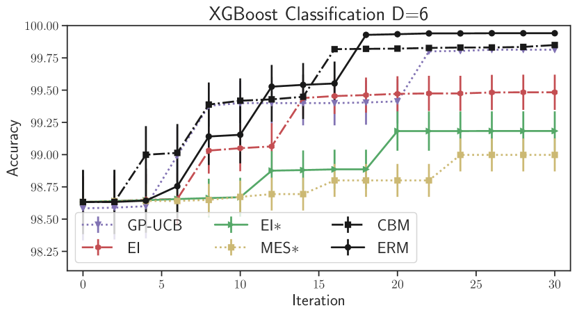
Figure 5: Tuning performance on Skin dataset.

The Skin Segmentation dataset is split into $15\%$ for training and $85\%$ for testing for a classification problem. There are $6$ hyperparameters for XGBoost (Chen & Guestrin, 2016) which is summarized in Table 1. To optimize the integer (ordinal) variables, we round the scalars to the nearest values in the continuous space. We present the result in Fig. 5. Our proposed ERM is the best approach, outperforming all the baselines by a wide margin. This demonstrates the benefit of exploiting the optimum value $f^{*}$ in BO.

Deep reinforcement learning.

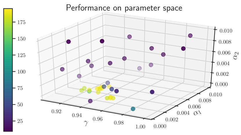
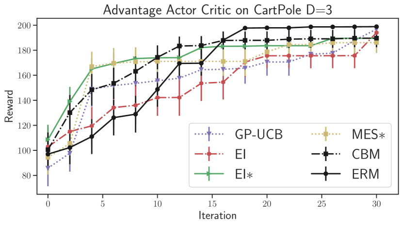
Figure 6: Hyperparameter tuning for a deep reinforcement learning algorithm. The optimum value is available $f^{*}=200$. Left: Selected points by our algorithm on tuning DRL. Color indicates the reward $f(x)$ value. Right: Performance comparison with the baselines.

CartPole is a pendulum with a center of gravity above its pivot point. The goal is to keep the cartpole balanced by controlling a pivot point. The reward performance in CartPole is often averaged over $100$ consecutive trials. The maximum reward is known from the literature as $f^{*}=200$.

We then use a deep reinforcement learning (DRL) algorithm to solve the CartPole problem and use Bayesian optimization to optimize the hyperparameters. In particular, we use the advantage actor critic (A2C) (Sutton & Barto, 1998) which possesses three sensitive hyperparameters, including the discount factor $\gamma$, the learning rate for actor model, $\alpha_{1}$, and the learning rate for critic model, $\alpha_{2}$. We choose not to optimize the deep learning architecture for simplicity. We use Bayesian optimization given the known optimum output of $200$ to find the best hyperparameters for the A2C algorithm. We present the results in Fig. 6 where our ERM reaches the optimal performance after $20$ iterations outperforming all other baselines. In Fig. 6 Left, we visualize the selected point $\{\mathbf{x}_{t}\}_{t=1}^{T}$ by our ERM acquisition function. Our ERM initially explores at several places and then exploits in the high value region (yellow dots).

4.3 What happens if we misspecify the optimum value

We now consider setting the $f^{*}$ to a value which is not the true optimum of the black-box function. We show that our model’s performance will drop with misspecified value of $f^{*}$ with different effects. Specifically, we both set $f^{*}$ larger (over-specify) and smaller (under-specify) than the true value in a maximization problem.

We experiment with our ERM using this misspecified setting of $f^{*}$ in Fig. 7.

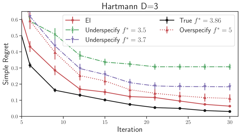
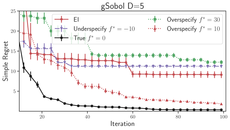
Figure 7: Experiments with ERM in the maximization problem. Over-specifying is when the value of $f^{*}$ is larger than the true optimal value and under-specifying is when the value of $f^{*}$ is smaller than the true. Top: the true $f^{*}=3.86$ for Hartmann. Bottom: the true $f^{*}=0$ for gSobol. Both cases of misspecifying $f^{*}$ will degrade the performance.

The results suggest that our algorithm using the true value ($f^{*}=3.86$ for Hartmann and $f^{*}=0$ for gSobol) will have the best performance. Both over-specifying and under-specifying $f^{*}$ will return worse performance. These misspecified settings slightly perform worse than the standard EI in Hartmann while it still performs better than EI for overspecifying $f^{*}=10$ in gSobol. In particular, the under-specifying case will result in worse performance than over-specifying. This is because our acquisition function will get stuck at the area once being found wrongly as the optimal. On the other hand, if we over-specify $f^{*}$, our algorithm continues exploring to find the optimum because it can not find the point where both conditions are met $\sigma(\mathbf{x}_{t})=0$ and $f^{*}=\mu(\mathbf{x}_{t})$.

Discussion.

We make the following observations. If we know the true value $f^{*}$, ERM will return the best result. If we do not know the exact $f^{*}$ value, the performance of our approach is degraded. Thus, we should use the existing BO approaches, such as EI, for the best performance.

5 Conclusion and Future Work

In this paper, we have considered a new setting in Bayesian optimization with known optimum output. We present a transformed Gaussian process surrogate to model the objective function better by exploiting the knowledge of $f^{*}$. Then, we propose two decision strategies which can exploit the function optimum value to make informed decisions. Our approaches are intuitively simple and easy to implement. By using extra knowledge of $f^{*}$, we demonstrate that our ERM can converge quickly to the optimum in benchmark functions and real-world applications.

In future work, we can expand our algorithm to handle batch setting for parallel evaluations or extend this work to other classes of surrogate functions such as Bayesian neural networks (Neal, 2012) and deep GP (Damianou & Lawrence, 2013). Moreover, we can extend the model to handle $f^{*}$ within a range of $\epsilon$ from the true output.

Appendix A Expected Regret Minimization Derivation

We are given an optimization problem $\mathbf{x}^{*}=\arg\max_{\mathbf{x}\in\mathcal{X}}f(\mathbf{x})$ where $f$ is a black-box function that we can evaluate pointwise. Let $\mathcal{D}_{t}=\left\{\mathbf{x}_{i}\in\mathcal{X},y_{i}\in\mathcal{R}\right\}_{i=1}^{t}$ be the observation set including an input $\mathbf{x}_{i}$, an outcome $y_{i}$ and $\mathcal{X}\in\mathcal{R}^{d}$ be the bounded search space. We define the regret function $r\left(\mathbf{x}\right)=f^{*}-f(\mathbf{x})$ where $f^{*}=\max_{\mathbf{x}\in\mathcal{X}}f(\mathbf{x})$ is the known global optimum value. The likelihood of the regret $r\left(\mathbf{x}\right)$ on a normal posterior distribution is as follows

$$p\left(r(\mathbf{x})\right)= \frac{1}{\sqrt{2\pi}\sigma\left(\mathbf{x}\right)}\exp\left(-\frac{1}{2}\frac{\left[\mu\left(\mathbf{x}\right)-f^{*}+r(\mathbf{x})\right]^{2}}{\sigma^{2}\left(\mathbf{x}\right)}\right).$$ (9)

The expected regret can be written using the likelihood function in Eq. (9), we obtain $\mathbb{E}\left[r\left(\mathbf{x}\right)\right]$

$$=\int_{0}^{\infty}\frac{r(\mathbf{x})}{\sqrt{2\pi}\sigma\left(\mathbf{x}\right)}\exp\left(-\frac{1}{2}\frac{\left[\mu\left(\mathbf{x}\right)-f^{*}+r(\mathbf{x})\right]^{2}}{\sigma^{2}\left(\mathbf{x}\right)}\right)dr(\mathbf{x}).$$

As the ultimate goal in optimization is to minimize the regret, we consider our acquisition function to minimize this expected regret as $\alpha^{\textrm{ERM}}\left(\mathbf{x}\right)=\mathbb{E}\left[r\left(\mathbf{x}\right)\right]$. Let $t=\frac{\mu\left(\mathbf{x}\right)-f^{*}+r(\mathbf{x})}{\sigma\left(\mathbf{x}\right)}$, then $r(\mathbf{x})=t\times\sigma\left(\mathbf{x}\right)-\mu(\mathbf{x})+f^{*}$ and $dt=\frac{dr}{\sigma\left(\mathbf{x}\right)}$. We write $\alpha^{\textrm{ERM}}\left(\mathbf{x}\right)$

$$= \int_{t=\frac{\mu\left(\mathbf{x}\right)-f^{*}}{\sigma\left(\mathbf{x}\right)}}^{\infty}\frac{t\times\sigma\left(\mathbf{x}\right)+f^{*}-\mu\left(\mathbf{x}\right)}{\sqrt{2\pi}}\exp(-\frac{1}{2}t^{2})dt$$

$$= \sigma\left(\mathbf{x}\right)\int_{t=\frac{\mu\left(\mathbf{x}\right)-f^{*}}{\sigma\left(\mathbf{x}\right)}}^{\infty}\frac{t}{\sqrt{2\pi}}\exp(-\frac{1}{2}t^{2})dt$$

$$+\left[f^{*}-\mu\left(\mathbf{x}\right)\right]\int_{t=\frac{\mu\left(\mathbf{x}\right)-f^{*}}{\sigma\left(\mathbf{x}\right)}}^{\infty}\frac{1}{\sqrt{2\pi}}\exp(-\frac{1}{2}t^{2})dt.$$ (10)

We compute the first term in Eq. (10) as

$$\sigma\left(\mathbf{x}\right)\int_{t=\frac{\mu\left(\mathbf{x}\right)-f^{*}}{\sigma\left(\mathbf{x}\right)}}^{\infty}\frac{t}{\sqrt{2\pi}}\exp(-\frac{1}{2}t^{2})dt$$

$$=\frac{\sigma\left(\mathbf{x}\right)}{\sqrt{2\pi}}\left[-\exp\left(-\frac{1}{2}\left[\frac{\mu\left(\mathbf{x}\right)-f^{*}+r(\mathbf{x})}{\sigma\left(\mathbf{x}\right)}\right]^{2}\right)\right]_{r=0}^{r=\infty}$$

$$=\sigma(\mathbf{x})\mathcal{N}\left(\frac{\mu\left(\mathbf{x}\right)-f^{*}}{\sigma\left(\mathbf{x}\right)}\mid 0,1\right).$$

Next, we compute the second term in Eq. (10) as

$$\left[f^{*}-\mu\left(\mathbf{x}\right)\right]\int_{t=\frac{\mu\left(\mathbf{x}\right)-f^{*}}{\sigma\left(\mathbf{x}\right)}}^{\infty}\frac{1}{\sqrt{2\pi}}\exp(-\frac{1}{2}t^{2})dt$$

$$=\left[f^{*}-\mu\left(\mathbf{x}\right)\right]\left\{\int_{-\infty}^{\infty}\mathcal{N}\left(t\mid 0,1\right)dt-\int_{-\infty}^{\frac{\mu\left(\mathbf{x}\right)-f^{*}}{\sigma\left(\mathbf{x}\right)}}\mathcal{N}\left(t\mid 0,1\right)dt\right\}$$

$$=\left[f^{*}-\mu\left(\mathbf{x}\right)\right]\left[1-\Phi\left(\frac{\mu\left(\mathbf{x}\right)-f^{*}}{\sigma\left(\mathbf{x}\right)}\right)\right]$$

$$=\left[f^{*}-\mu\left(\mathbf{x}\right)\right]\Phi\left(\frac{f^{*}-\mu\left(\mathbf{x}\right)}{\sigma\left(\mathbf{x}\right)}\right).$$

Let $z=\frac{f^{*}-\mu\left(\mathbf{x}\right)}{\sigma\left(\mathbf{x}\right)}$, we obtain the acquisition function

$$\alpha^{\textrm{ERM}}\left(\mathbf{x}\right) =\sigma\left(\mathbf{x}\right)\phi\left(z\right)+\left[f^{*}-\mu\left(\mathbf{x}\right)\right]\Phi\left(z\right)$$ (11)

where $\phi\left(z\right)=\mathcal{N}\left(z\mid 0,1\right)$ is the standard normal pdf and $\Phi\left(z\right)$ is the cdf. To select the next point, we minimize this acquisition function which is equivalent to minimize the expected regret $\mathbb{E}\left[r\left(\mathbf{x}\right)\right]$

$$\mathbf{x}_{t+1} =\arg\min_{\mathbf{x}\in\mathcal{X}}\alpha^{\textrm{ERM}}\left(\mathbf{x}\right)=\arg\min_{\mathbf{x}\in\mathcal{X}}\mathbb{E}\left[r\left(\mathbf{x}\right)\right].$$

We can see that this acquisition function is minimized $\alpha^{\textrm{ERM}}\left(\mathbf{x}_{t}\right)=\mathbb{E}[r(\mathbf{x}_{t})]=0$ when $f^{*}=\mu(\mathbf{x}_{t})$ and $\sigma(\mathbf{x}_{t})=0$. Our chosen point $\mathbf{x}_{t}$ is the one which offers the smallest expected regret. We aim to find the point with the desired property of $\mathbb{E}[r(\mathbf{x}_{t})]=0$.

Appendix B Additional Experiments

We first illustrate the BO with and without the knowledge of $f^{*}$. Then, we provide additional information about the deep reinforcement learning experiment in the main paper. Next, we compare the effect of using the vanilla GP and transformed GP with different acquisition functions.

B.1 Illustration per iteration

We provide the illustration of BO with and without the knowledge of $f^{*}$ for comparison in Figs. 8 and 9. We show the GP and EI in the left (without $f^{*}$) and the transformed GP and ERM in the right (with $f^{*}$). As the effect of transformation using $f^{*}$, the transformed GP (right) can lift up the surrogate model closer to the true value $f^{*}$ (red horizontal line) encouraging the acquisition function to select at these potential locations. On the other hand, without $f^{*}$, the GP surrogate (left) is less informative. As a result, the EI operating on GP (left) is less efficient as opposed to the transformed GP. We demonstrate visually that using TGP our model can finally find the optimum input within the evaluation budget while the standard GP does not.

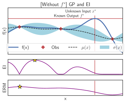
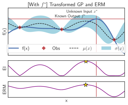
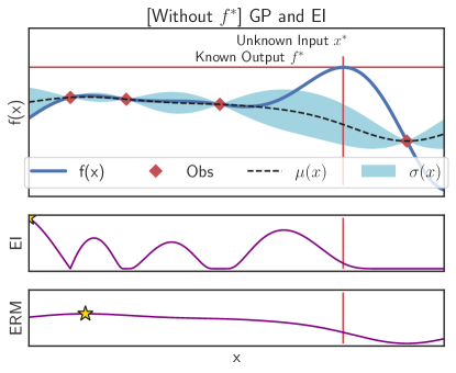
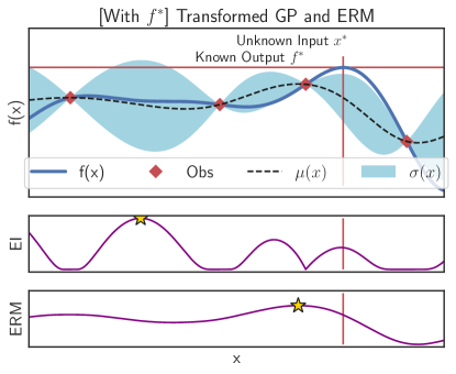
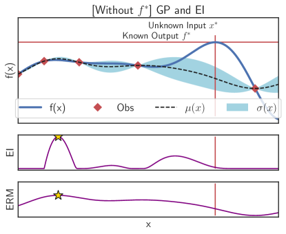
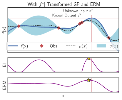
Figure 8: Illustration of the optimization process per iteration $1-3$ starting given the same initialization. Left: BO using GP as surrogate and EI as acquisition function. Right: BO using TGP as surrogate and ERM as acquisition function. Given the known optimum $f^{*}$ value, the transformed GP can lift up the surrogate model closer to the known value. Then, the ERM will make informed decision given $f^{*}$. We also show that the EI may not make the best decision as ERM. To be continue in the next figure.

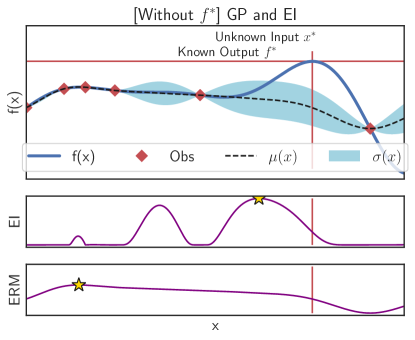
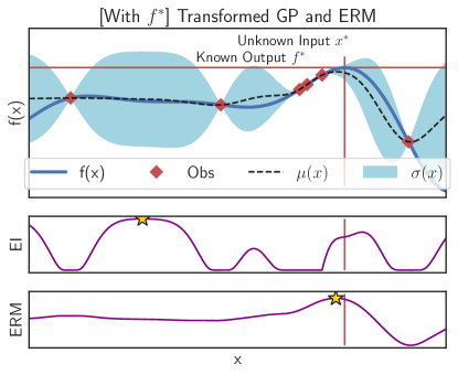
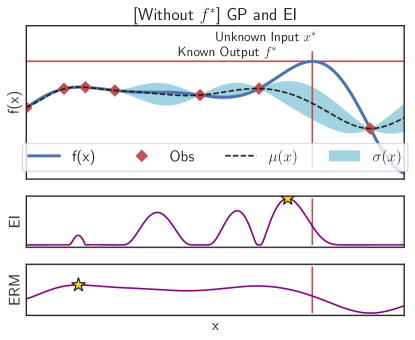
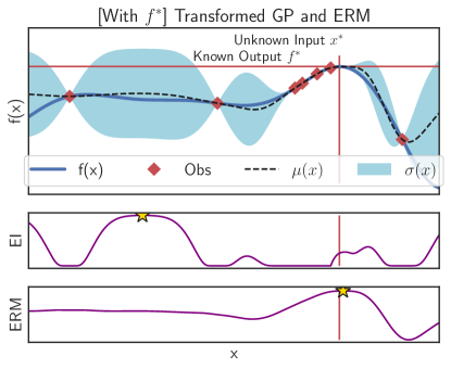
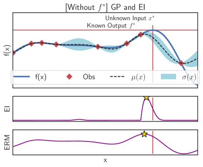
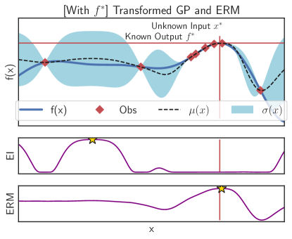
Figure 9: Continuing from the previous figure. Illustration of the optimization process per iteration $4-6$ starting given the same initialization. Left: BO using GP as surrogate and EI as acquisition function. Right: BO using TGP as surrogate and ERM as acquisition function. Given the known optimum $f^{*}$ value, the transformed GP can lift up the surrogate model closer to the known value. Then, the ERM will make informed decision given $f^{*}$. We also show that the EI may not make the best decision as ERM.

B.2 Details of A2C on CartPole problem

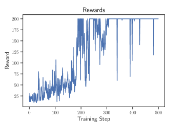
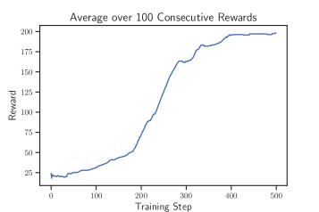
Figure 10: Left: visualization of a CartPole. Middle and Right: visualization of the reward curve using the best found parameter value $\mathbf{x}^{*}$. We have used the Advantage Actor Critic (A2C) algorithm to solve the CartPole problem. The known optimum value is $f^{*}=200$.

We use the advantage actor critic (A2C) (Sutton & Barto, 1998) as the deep reinforcement learning algorithm to solve the CartPole problem (Barto et al., 1983). This A2C is implemented in Tensorflow Abadi et al. (2016) and run on a NVIDIA GTX 2080 GPU machine. In A2C, we use two neural network models to learn $Q(s,a)$ and $V(s)$ separately. In particular, we use a simple neural network architecture with $2$ layers and $10$ nodes in each layer. The range of the used hyperparameters in A2C and the found optimal parameter are summarized in Table 2.

We illustrate the reward performance over $500$ training episodes using the found optimal parameter $\mathbf{x}^{*}=\underset{{}_{\mathbf{x}\in\mathcal{X}}}{\text{argmax}}f(\mathbf{x})$ value in Fig. 10. In particular, we plot the raw reward and the average reward over 100 consecutive episodes - this average score is used as the evaluation output. Our A2C with the found hyperparameter will take around $300$ episodes to reach the optimum value $f^{*}=200$.

Table 2: Hyperparameters of Advantage Actor Critic.

Variables	Min	Max	Best Parameter $\mathbf{x}^{*}$
$\gamma$ discount factor	$0.9$	$1$	$0.95586$
learning rate $q$ model	$1e^{-6}$	$0.01$	$0.00589$
learning rate $v$ model	$1e^{-6}$	$0.01$	$0.00037$

B.3 Comparison using vanilla GP and transformed GP

We empirically compare the proposed transformed Gaussian process (using the knowledge of $f^{*})$ and the vanilla Gaussian process (Rasmussen, 2006) as the surrogate model for Bayesian optimization. We then test our ERM and EI on the two surrogate models. After the experiment, we learn that the transformed GP is more suitable for our ERM while it may not be ideal for the EI.

ERM.

We perform experiments on ERM acquisition function using two surrogate models as vanilla Gaussian process (GP) and transformed Gaussian process (TGP). Our acquisition function performs better with the TGP. The TGP exploits the knowledge about the optimum value $f^{*}$ to construct the surrogate model. Thus, it is more informative and can be helpful in high dimension functions, such as Alpine1 $D=5$ and gSobol $D=5$, $D=10$, in which the ERM on TGP achieves much better performance than ERM on GP. On the simpler functions, such as branin and hartmann, the transformed GP surrogate achieves comparable performances with the vanilla GP. We visualize all results in Fig. 11.

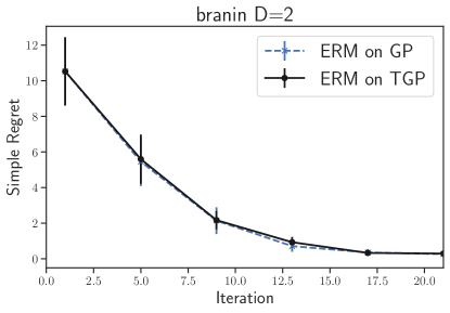
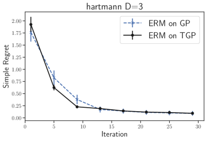
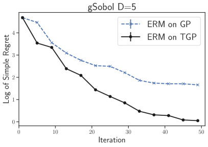
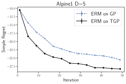
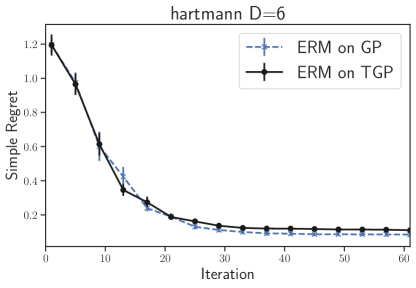
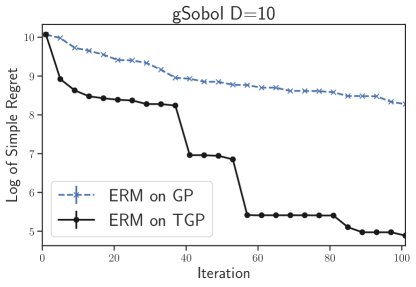
Figure 11: Experiments with ERM acquisition function on vanilla Gaussian process (GP) and transformed Gaussian process (TGP). Our acquisition function using the transformed GP consistently performs better than using the vanilla GP. Particularly, the TGP will be more useful in high-dimensional functions of Alpine1 $D=5$ and gSobol $D=5$, $D=10$ functions. In these functions, ERM on TGP will outperform ERM on GP by a wide margin.

Expected Improvement (EI).

We then test the EI acquisition function on two surrogate models of vanilla Gaussian process and our transformed Gaussian process (using $f^{*}$) in Fig. 12. In contrast to the case of ERM above, we show that the EI will perform well on the vanilla GP, but not on the TGP. This can be explained by the side effect of the GP transformation as follows. From Eq. (1) in the main paper, when the location has poor (or low) prediction value $\mu(\mathbf{x})=f^{*}-\frac{1}{2}\mu_{g}^{2}(\mathbf{x})$, we will have large value $\mu_{g}(\mathbf{x})$. As a result, this large value of $\mu_{g}(\mathbf{x})$ will make the uncertainty larger $\sigma(\mathbf{x})=\mu_{g}(\mathbf{x})\sigma_{g}(\mathbf{x})\mu_{g}(\mathbf{x})$ from Eq. (2) in the main paper. Therefore, TGP will make an additional uncertainty $\sigma(\mathbf{x})$ at the location where $\mu(\mathbf{x})$ is low.

Under the additional uncertainty effect of TGP, the expected improvement may spend more iterations to explore these uncertainty area and take more time to converge than the case of using the vanilla GP. We note that this effect will also happen to the GP-UCB and other acquisition functions, which rely on exploration-exploitation trade-off.

In high dimensional function of gSobol $D=10$, TGP will make the EI explore aggressively due to the high uncertainty effect (described above) and thus result in worse performance. That is, it keeps exploring at poor region in the first $100$ iterations (see bottom row of Fig. 12).

Discussion.

The transformed Gaussian process (TGP) surrogate takes into account the knowledge of optimum value $f^{*}$ to inform the surrogate. However, this transformation may create additional uncertainty at the area where function value is low. While our proposed acquisition function ERM and CBM will not suffer this effect, the existing acquisition functions of EI and UCB will. Therefore, we only recommend to use this TGP with our acquisition functions for the best optimization performance.

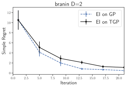
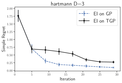
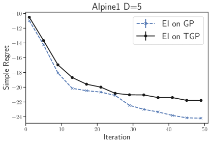
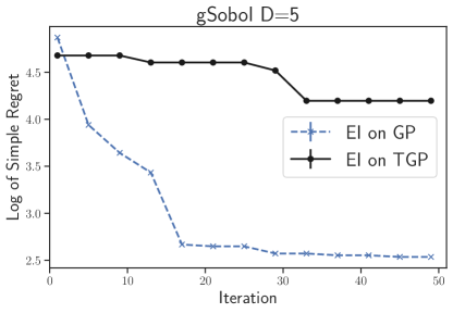
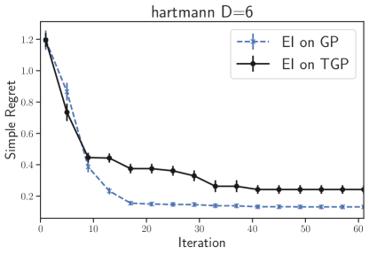
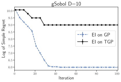
Figure 12: Experiments with EI acquisition function using the surrogate models as GP and TGP. Although the TGP exploits the knowledge about the optimum value $f^{*}$ to construct the informed surrogate model, it brings the side effect of transformation in making additional GP predictive uncertainty. As a result, the EI will explore more aggressively using TGP and thus obtain worse performance comparing to the case of using vanilla GP.

Appendix C Other known optimum value settings

To highlight the applicability of the proposed model, we list several other settings where the optimum values are known in Table 3.

Table 3: Examples of known optimum value settings.

Environment	$f^{*}$	Source
Pong	$18$	Gym.OpenAI
Frozen Lake	$0.79$	Gym.OpenAI
Inverted Pendulum v1	$135.91$	Gym.OpenAI
CartPole	$200$	Gym.OpenAI

References

- Abadi et al. (2016) Abadi, M., Barham, P., Chen, J., Chen, Z., Davis, A., Dean, J., Devin, M., Ghemawat, S., Irving, G., Isard, M., et al. Tensorflow: A system for large-scale machine learning. In 12th Symposium on Operating Systems Design and Implementation (OSDI 16), pp. 265–283, 2016.
- Ahuja & Orlin (2001) Ahuja, R. K. and Orlin, J. B. Inverse optimization. Operations Research, 49(5):771–783, 2001.
- Astudillo & Frazier (2019) Astudillo, R. and Frazier, P. Bayesian optimization of composite functions. In International Conference on Machine Learning, pp. 354–363, 2019.
- Barto et al. (1983) Barto, A. G., Sutton, R. S., and Anderson, C. W. Neuronlike adaptive elements that can solve difficult learning control problems. IEEE transactions on systems, man, and cybernetics, (5):834–846, 1983.
- Berk et al. (2018) Berk, J., Nguyen, V., Gupta, S., Rana, S., and Venkatesh, S. Exploration enhanced expected improvement for Bayesian optimization. In Machine Learning and Knowledge Discovery in Databases. Springer, 2018.
- Brochu et al. (2010) Brochu, E., Cora, V. M., and De Freitas, N. A tutorial on Bayesian optimization of expensive cost functions, with application to active user modeling and hierarchical reinforcement learning. arXiv preprint arXiv:1012.2599, 2010.
- Chen & Guestrin (2016) Chen, T. and Guestrin, C. Xgboost: A scalable tree boosting system. In Proceedings of the 22nd acm sigkdd international conference on knowledge discovery and data mining, pp. 785–794. ACM, 2016.
- Chen et al. (2018) Chen, Y., Huang, A., Wang, Z., Antonoglou, I., Schrittwieser, J., Silver, D., and de Freitas, N. Bayesian optimization in AlphaGo. arXiv preprint arXiv:1812.06855, 2018.
- Damianou & Lawrence (2013) Damianou, A. and Lawrence, N. Deep gaussian processes. In Artificial Intelligence and Statistics, pp. 207–215, 2013.
- Frazier & Wang (2016) Frazier, P. I. and Wang, J. Bayesian optimization for materials design. In Information Science for Materials Discovery and Design, pp. 45–75. Springer, 2016.
- Gopakumar et al. (2018) Gopakumar, S., Gupta, S., Rana, S., Nguyen, V., and Venkatesh, S. Algorithmic assurance: An active approach to algorithmic testing using Bayesian optimisation. In Advances in Neural Information Processing Systems (NeurIPS), pp. 5465–5473, 2018.
- Gunter et al. (2014) Gunter, T., Osborne, M. A., Garnett, R., Hennig, P., and Roberts, S. J. Sampling for inference in probabilistic models with fast Bayesian quadrature. In Advances in neural information processing systems, pp. 2789–2797, 2014.
- Hennig & Schuler (2012) Hennig, P. and Schuler, C. J. Entropy search for information-efficient global optimization. Journal of Machine Learning Research, 13:1809–1837, 2012.
- Hernández-Lobato & Hernández-Lobato (2016) Hernández-Lobato, D. and Hernández-Lobato, J. M. Scalable Gaussian process classification via expectation propagation. In Artificial Intelligence and Statistics, pp. 168–176, 2016.
- Hernández-Lobato et al. (2014) Hernández-Lobato, J. M., Hoffman, M. W., and Ghahramani, Z. Predictive entropy search for efficient global optimization of black-box functions. In Advances in Neural Information Processing Systems, pp. 918–926, 2014.
- Hernández-Lobato et al. (2017) Hernández-Lobato, J. M., Requeima, J., Pyzer-Knapp, E. O., and Aspuru-Guzik, A. Parallel and distributed Thompson sampling for large-scale accelerated exploration of chemical space. In International Conference on Machine Learning, pp. 1470–1479, 2017.
- Hoffman & Ghahramani (2015) Hoffman, M. W. and Ghahramani, Z. Output-space predictive entropy search for flexible global optimization. 2015.
- Hutter et al. (2011) Hutter, F., Hoos, H. H., and Leyton-Brown, K. Sequential model-based optimization for general algorithm configuration. In Learning and Intelligent Optimization, pp. 507–523. Springer, 2011.
- Klein et al. (2017) Klein, A., Falkner, S., Bartels, S., Hennig, P., and Hutter, F. Fast Bayesian optimization of machine learning hyperparameters on large datasets. In Artificial Intelligence and Statistics, pp. 528–536, 2017.
- Kuss & Rasmussen (2005) Kuss, M. and Rasmussen, C. E. Assessing approximate inference for binary Gaussian process classification. Journal of machine learning research, 6(Oct):1679–1704, 2005.
- Le et al. (2016) Le, T., Nguyen, V., Nguyen, T. D., and Phung, D. Nonparametric budgeted stochastic gradient descent. In Proceedings of the 19th International Conference on Artificial Intelligence and Statistics, pp. 654–572, 2016.
- Letham et al. (2019) Letham, B., Karrer, B., Ottoni, G., Bakshy, E., et al. Constrained Bayesian optimization with noisy experiments. Bayesian Analysis, 14(2):495–519, 2019.
- Li et al. (2018) Li, C., Santu, R., Gupta, S., Nguyen, V., Venkatesh, S., Sutti, A., Leal, D. R. D. C., Slezak, T., Height, M., Mohammed, M., and Gibson, I. Accelerating experimental design by incorporating experimenter hunches. In IEEE International Conference on Data Mining (ICDM), pp. 257–266, 2018.
- MacKay (1998) MacKay, D. J. Introduction to Gaussian processes. NATO ASI Series F Computer and Systems Sciences, 168:133–166, 1998.
- Mockus et al. (1978) Mockus, J., Tiesis, V., and Zilinskas, A. The application of Bayesian methods for seeking the extremum. Towards global optimization, 2(117-129):2, 1978.
- Neal (2012) Neal, R. M. Bayesian learning for neural networks, volume 118. Springer Science & Business Media, 2012.
- Nguyen et al. (2019) Nguyen, V., Gupta, S., Rana, S., Thai, M., Li, C., and Venkatesh, S. Efficient Bayesian optimization for uncertainty reduction over perceived optima locations. In IEEE 19th International Conference on Data Mining (ICDM), 2019.
- Nickisch & Rasmussen (2008) Nickisch, H. and Rasmussen, C. E. Approximations for binary Gaussian process classification. Journal of Machine Learning Research, 9(Oct):2035–2078, 2008.
- Oh et al. (2018) Oh, C., Gavves, E., and Welling, M. Bock: Bayesian optimization with cylindrical kernels. In International Conference on Machine Learning, pp. 3865–3874, 2018.
- Osborne et al. (2012) Osborne, M., Garnett, R., Ghahramani, Z., Duvenaud, D. K., Roberts, S. J., and Rasmussen, C. E. Active learning of model evidence using Bayesian quadrature. In Advances in neural information processing systems, pp. 46–54, 2012.
- Perdikaris & Karniadakis (2016) Perdikaris, P. and Karniadakis, G. E. Model inversion via multi-fidelity bayesian optimization: a new paradigm for parameter estimation in haemodynamics, and beyond. Journal of The Royal Society Interface, 13(118):20151107, 2016.
- Rasmussen (2006) Rasmussen, C. E. Gaussian processes for machine learning. 2006.
- Riihimäki et al. (2013) Riihimäki, J., Jylänki, P., and Vehtari, A. Nested expectation propagation for Gaussian process classification with a multinomial probit likelihood. Journal of Machine Learning Research, 14(Jan):75–109, 2013.
- Ru et al. (2018) Ru, B., McLeod, M., Granziol, D., and Osborne, M. A. Fast information-theoretic Bayesian optimisation. In International Conference on Machine Learning, pp. 4381–4389, 2018.
- Ru et al. (2020) Ru, B., Alvi, A. S., Nguyen, V., Osborne, M. A., and Roberts, S. J. Bayesian optimisation over multiple continuous and categorical inputs. In International Conference on Machine Learning, 2020.
- Shahriari et al. (2016) Shahriari, B., Swersky, K., Wang, Z., Adams, R. P., and de Freitas, N. Taking the human out of the loop: A review of Bayesian optimization. Proceedings of the IEEE, 104(1):148–175, 2016.
- Snelson et al. (2004) Snelson, E., Ghahramani, Z., and Rasmussen, C. E. Warped Gaussian processes. In Advances in neural information processing systems, pp. 337–344, 2004.
- Snoek et al. (2012) Snoek, J., Larochelle, H., and Adams, R. P. Practical Bayesian optimization of machine learning algorithms. In Advances in neural information processing systems, pp. 2951–2959, 2012.
- Snoek et al. (2015) Snoek, J., Rippel, O., Swersky, K., Kiros, R., Satish, N., Sundaram, N., Patwary, M., Prabhat, M., and Adams, R. Scalable Bayesian optimization using deep neural networks. In Proceedings of the 32nd International Conference on Machine Learning, pp. 2171–2180, 2015.
- Springenberg et al. (2016) Springenberg, J. T., Klein, A., Falkner, S., and Hutter, F. Bayesian optimization with robust bayesian neural networks. In Advances in Neural Information Processing Systems, pp. 4134–4142, 2016.
- Srinivas et al. (2010) Srinivas, N., Krause, A., Kakade, S., and Seeger, M. Gaussian process optimization in the bandit setting: No regret and experimental design. In Proceedings of the 27th International Conference on Machine Learning, pp. 1015–1022, 2010.
- Sutton & Barto (1998) Sutton, R. S. and Barto, A. G. Reinforcement learning: An introduction, volume 1. MIT press Cambridge, 1998.
- Wang & de Freitas (2014) Wang, Z. and de Freitas, N. Theoretical analysis of Bayesian optimisation with unknown Gaussian process hyper-parameters. arXiv preprint arXiv:1406.7758, 2014.
- Wang & Jegelka (2017) Wang, Z. and Jegelka, S. Max-value entropy search for efficient Bayesian optimization. In International Conference on Machine Learning, pp. 3627–3635, 2017.
- Wang et al. (2016) Wang, Z., Zhou, B., and Jegelka, S. Optimization as estimation with Gaussian processes in bandit settings. In Proceedings of the 19th International Conference on Artificial Intelligence and Statistics, pp. 1022–1031, 2016.
- Wang et al. (2018) Wang, Z., Gehring, C., Kohli, P., and Jegelka, S. Batched large-scale Bayesian optimization in high-dimensional spaces. In International Conference on Artificial Intelligence and Statistics, pp. 745–754, 2018.