High Frequency Residual Learning for Multi-Scale Image Classification

Abstract

We present a novel high frequency residual learning framework, which leads to a highly efficient multi-scale network (MSNet) architecture for mobile and embedded vision problems. The architecture utilizes two networks: a low resolution network to efficiently approximate low frequency components and a high resolution network to learn high frequency residuals by reusing the upsampled low resolution features. With a classifier calibration module, MSNet can dynamically allocate computation resources during inference to achieve a better speed and accuracy trade-off. We evaluate our methods on the challenging ImageNet-1k dataset and observe consistent improvements over different base networks. On ResNet-18 and MobileNet with $\alpha=1.0$, MSNet gains 1.5% accuracy over both architectures without increasing computations. On the more efficient MobileNet with $\alpha=0.25$, our method gains 3.8% accuracy with the same amount of computations.

1 Introduction

(a)	(b)	(c)	(d)

Figure 1: Frequency domain analysis. We visualize the magnitude of 2D discrete Fourier transform of final feature map of different networks. We plot the average magnitude of all feature maps from the last convolutional layer. (a): input image to the network. (b): mean magnitude for ResNet-18, it contains mostly the low frequency component. (c): mean magnitude for low resolution network of MS-ResNet-18, compared with ResNet-18, its low frequency component is more concentrated to the DC component. (d): mean magnitude for high resolution network of MS-ResNet-18, compared with ResNet-18 and its low resolution counterpart, it has far less low frequency component. The red ellipse partially covers the high frequency region. From ResNet-18, it shows strong high frequency magnitude. From lower resolution network of MS-ResNet-18, the covered frequency vanishes; while the higher resolution network recovers the high frequency.

Convolutional neural networks (CNNs) have become the dominant machine learning approach in solving computer vision problems such as, image classification [Krizhevsky et al.(2012)Krizhevsky, Sutskever, and Hinton, Simonyan and Zisserman(2014), Szegedy et al.()Szegedy, Liu, Jia, Sermanet, Reed, Anguelov, Erhan, Vanhoucke, Rabinovich, Rick Chang, et al., He et al.(2016)He, Zhang, Ren, and Sun, Cheng et al.(2018b)Cheng, Wei, Shi, Chang, Xiong, and Huang, Cheng et al.(2018e)Cheng, Xiao, Guo, Hu, Wang, and Zhang], object detection [Girshick et al.(2014)Girshick, Donahue, Darrell, and Malik, Girshick(2015), Ren et al.(2015)Ren, He, Girshick, and Sun, Cheng et al.(2018d)Cheng, Wei, Shi, Feris, Xiong, and Huang, Wei et al.(2018)Wei, Shen, Cheng, Shi, Xiong, Feng, and Huang, Cheng et al.(2018c)Cheng, Wei, Shi, Feris, Xiong, and Huang], semantic segmentation [Long et al.(2015)Long, Shelhamer, and Darrell, Chen et al.(2018a)Chen, Papandreou, Kokkinos, Murphy, and Yuille, Zhao et al.(2017)Zhao, Shi, Qi, Wang, and Jia, Chen et al.(2017a)Chen, Papandreou, Schroff, and Adam, Chen et al.(2018b)Chen, Zhu, Papandreou, Schroff, and Adam], etc. In the past several years, great progresses have been achieved in the study of developing large and computationally intensive networks [Simonyan and Zisserman(2014), He et al.(2016)He, Zhang, Ren, and Sun, Szegedy et al.(2017)Szegedy, Ioffe, Vanhoucke, and Alemi] to achieve higher accuracy with the cost of sacrificing speed and efficiency.

Meanwhile, there have been increasing needs of deploying convolutional neural networks into mobile devices with limited computational resources. To address the computational efficiency problem, works [Howard et al.(2017)Howard, Zhu, Chen, Kalenichenko, Wang, Weyand, Andreetto, and Adam, Zhang et al.(2017)Zhang, Zhou, Lin, and Sun, Sandler et al.(2018)Sandler, Howard, Zhu, Zhmoginov, and Chen] have been proposed to discover more efficient network structure. Common strategies such as replacing convolution operation with more efficient group or depth-wise separable convolutions, using less channels and using lower resolution input have been used.

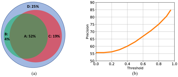
Among these strategies, reducing the input resolution by half is probably the simplest method with the advantage that it can be directly applied during inference. Without the need of re-training, it can reduce the computation cost quadratically. However, while it decreases the computational cost, it usually scarifies the overall accuracy. One question we want to ask and address is: can we do inference on low resolution images without losing accuracy? The answer is yes for some images but not for all the images. Recent works [Wang et al.(2016)Wang, Chang, Yang, Liu, and Huang, Cheng et al.(2017)Cheng, Wang, Zhang, Li, Liu, Yang, Huang, and Huang, Liu et al.(2017)Liu, Cheng, Wang, Zhang, and Huang, Cheng et al.(2018a)Cheng, Liu, Wang, Zhang, and Huang] propose to directly inference from low resolution input by integrating a super-resolution network with a classification network, but the gain is still marginal. We observe that there are some easy images that can be predicted correctly using both their low resolution and high resolution versions (Figure 2 (a)). A straightforward solution is to predict a low resolution image first. If the prediction is incorrect, we make another prediction using the high resolution image. This straightforward solution has a problem that we do not know when classifier fails on low resolution. However, based on the property of softmax function, we can make an assumption that when the prediction of a classifier has a high softmax score, it is more likely to be a correct prediction (Figure 2 (b)). Based on this assumption, we can develop a classifier calibration module: we first run prediction on low resolution images, if the softmax score of the prediction is higher than a threshold, we keep this prediction; if the softmax score of the prediction is lower than the threshold, we use the prediction on the high resolution image. Classifier calibration can be used dynamically during inference to save the average computation.

However, classifier calibration only solves the problem partially. While for an easy image we can use the low resolution predictor to save computational cost quadratically, for a hard image we need to use two predictors corresponding to low and high resolutions as we need the prediction score from the low resolution predictor to tell whether it is an easy or hard image. Checking this process closer, we can easily find that this naive solution does not reuse features of low resolution images anymore once it finishes the prediction on low resolution images, which leads to a waste of computation.

Therefore, the second question we want to ask and address is more intriguing: can low resolution features help high resolution predictions? This question is more interesting because reusing low resolution features will save more computational overheads.

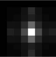
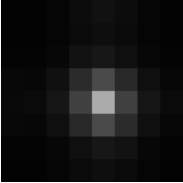
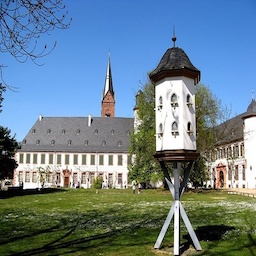
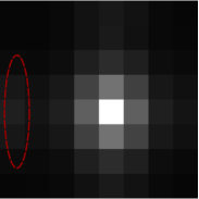
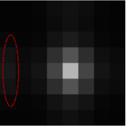
Inspired by the idea of wavelet transform and residual learning, we propose a novel network structure named High Frequency Residual Multi-Scale Network (MSNet) aiming at learning low frequency components and high frequency residuals separately. Note that a feature map normally contains both low frequency components and high frequency components (Figure 1 (b)). If we upsample a low resolution feature map, it contains mostly low frequency components (Figure 1 (c)). We find that by reusing the upsampled low resolution features, the network has the ability to learn high frequency residuals with less low frequency components (Figure 1 (d)). Formally, denoting the desired high resolution feature map by $\mathbf{y}_{H}$, we hope a lower scale network (a network takes as input low resolution images) learns mainly low frequency components $\mathbf{y}_{L}=\mathcal{L}(\mathbf{x}_{L})$ and a higher scale network (a network takes as input high resolution images) learns mainly high frequency residuals $\mathcal{H}(\mathbf{x}_{H})$. Then the combination of the upsampled low frequency components and high frequency residuals is the desired complete feature map $\mathbf{y}_{H}=\mathcal{H}(\mathbf{x}_{H})+u(\mathbf{y}_{L})$. Combining classifier calibration and high frequency residual learning, we achieve a much better computation and accuracy trade-off on multiple efficient networks.

Our contributions are threefold. 1) We propose the MSNet based on high frequency residual learning to efficiently reuse multi-scale features. 2) We propose a classifier calibration module that can dynamically allocate computations during inference. 3) Our proposed network achieves consistent gains over various architectures without increasing the amount of the computation.

2 Related Works

Efficient Networks. Much attention has been placed on efficient network design recently. Most common methods for designing efficient network or efficient inference are: to use more efficient model component, e.g. group convolutions or even depth-wise convolutions [Howard et al.(2017)Howard, Zhu, Chen, Kalenichenko, Wang, Weyand, Andreetto, and Adam, Zhang et al.(2017)Zhang, Zhou, Lin, and Sun, Sandler et al.(2018)Sandler, Howard, Zhu, Zhmoginov, and Chen]; to perform model compression to reduce parameters and computations [Iandola et al.(2016)Iandola, Han, Moskewicz, Ashraf, Dally, and Keutzer, Yu et al.(2018)Yu, Yang, Xu, Yang, and Huang, Yu and Huang(2019)]; to use quantization to reduce float32 operations to float16, integer or even binary operations [Rastegari et al.(2016)Rastegari, Ordonez, Redmon, and Farhadi]; to use knowledge distillation to transfer knowledge of a large network or an ensemble of networks to a small network [Hinton et al.(2015)Hinton, Vinyals, and Dean, Romero et al.(2014)Romero, Ballas, Kahou, Chassang, Gatta, and Bengio, Polino et al.(2018)Polino, Pascanu, and Alistarh]. In this work, we focus on the efficient network learning, especially, we target at reducing the computation by reducing the input resolution but preserve the accuracy at the same time. The other model compression/acceleration methods are orthogonal to our method and can further boost the performance.

Residual Learning. The idea of ResNet [He et al.(2016)He, Zhang, Ren, and Sun] is to add the bypass connection between components in a feed-forward network. It makes deeper networks easier to optimize and has been applied in a wide variety of works [Rastegari et al.(2016)Rastegari, Ordonez, Redmon, and Farhadi, Chollet(2016), Szegedy et al.(2017)Szegedy, Ioffe, Vanhoucke, and Alemi, Xie et al.(2017)Xie, Girshick, Dollár, Tu, and He]. [Chen et al.(2017b)Chen, Li, Xiao, Jin, Yan, and Feng] shows the equivalence of residual networks [He et al.(2016)He, Zhang, Ren, and Sun] and densely connected networks [Huang et al.(2017)Huang, Liu, Weinberger, and van der Maaten] and the authors propose a general form of residual learning with enhanced performance. Compared with ResNet, we explicitly focus on learning the high frequency residual information in a multi-scale network architecture, which allows us to easily allocate the computational cost to trade-off the accuracy. Another perspective is that ResNet learns residual in the image domain while our method targets to learn residual in the frequency domain.

Cascade Classifiers. Cascade classifiers have been widely use for efficient inference. The high level idea of cascade classifiers to classify an image with a sequence of classifiers where the earlier classifiers reject easier images which is called an “early exit”. The Viola Jones Algorithm [Viola and Jones(2004)] for face detection uses a hard cascade by Adaboost [Freund and Schapire(1997)], where multiple week classifiers take different features in a cascade manner. If any of the classifier in the sequence rejects a region, then the region will be classified as a non-facial region. A soft cascade classifier [Bourdev and Brandt(2005)] builds each weak classifier based on the output of all previous classifiers. In the context of deep learning, multiple works have studied the problem of “early exit” in a deep model [Teerapittayanon et al.(2016)Teerapittayanon, McDanel, and Kung, Bolukbasi et al.(2017)Bolukbasi, Wang, Dekel, and Saligrama, Huang et al.(2018)Huang, Chen, Li, Wu, van der Maaten, and Weinberger]. The idea is to inference using early stage features based on the computation budget, however, the problem is early stage features usually do not have high level semantics. In our work, we use the idea of “early exit”, but instead of building weak classifiers at early stage features, we build a weak classifier on a low resolution input. In this way, our method achieves a good trade-off between speed and high-level features.

Multi-Scale Network Design. Network designs, either by human [Simonyan and Zisserman(2014), He et al.(2016)He, Zhang, Ren, and Sun, Huang et al.(2017)Huang, Liu, Weinberger, and van der Maaten] or by architecture search [Zoph et al.(2018)Zoph, Vasudevan, Shlens, and Le, Real et al.(2018)Real, Aggarwal, Huang, and Le], mainly focus on finding more powerful building blocks, e.g. residual blocks in [He et al.(2016)He, Zhang, Ren, and Sun], densely connected blocks in [Huang et al.(2017)Huang, Liu, Weinberger, and van der Maaten] and machine searched blocks in [Zoph et al.(2018)Zoph, Vasudevan, Shlens, and Le, Real et al.(2018)Real, Aggarwal, Huang, and Le]. However, all these works use a single resolution input (e.g. $224\times 224$ or $299\times 299$), we find less works study the effect of using features with different resolutions in classification. Recently, there are works [Zhang et al.(2007)Zhang, Zelinsky, and Samaras, Pedersoli et al.(2015)Pedersoli, Vedaldi, Gonzalez, and Roca, Huang et al.(2018)Huang, Chen, Li, Wu, van der Maaten, and Weinberger, Newell et al.(2016)Newell, Yang, and Deng, Yang et al.(2017)Yang, Li, Ouyang, Li, and Wang, Xie et al.(2018)Xie, Wang, Zhang, Lai, Hong, and Qi, Sun et al.(2019)Sun, Xiao, Liu, and Wang] focusing on multi-scale design. Although MSDNet [Huang et al.(2018)Huang, Chen, Li, Wu, van der Maaten, and Weinberger] claims to be “multi-scale”, we find it is more similar to [Saxena and Verbeek(2016)] which is a wrapping of different networks into a single network. As far as we know, our work is one of the first to show that reusing low resolution feature helps high resolution prediction. We will give a more detailed comparison in the next section.

Figure 2: Multi-resolution inference results. The model is ResNet-18. (a): accuracy distribution from the input of $128\times 128$ and $256\times 256$. Region A: correctly predicted by both $128\times 128$ and $256\times 256$; Region B: correctly predicted by $128\times 128$ but incorrectly predicted by $256\times 256$; Region C: incorrectly predicted by $128\times 128$ but correctly predicted by $256\times 256$; Region D: incorrectly predicted by both $128\times 128$ and $256\times 256$. (b): precision vs thresholds. The threshold is used to select images to be predicted using low resolution input ($128\times 128$), precision is the accuracy of the selected image. The higher the threshold, the less images are selected and the accuracy becomes higher.

3 High Frequency Residual Learning

3.1 Analysis of Multi-Resolution Inference

Nowadays, most CNN model architecture are fully convolutional with a global average pooling as the last feature layer, making it straightforward to do inference at arbitrary resolution. Given a well-trained model, we can evaluate its inference accuracy over different scales. Figure 2 shows the experiment results. The dataset is ImageNet 2012 [Deng et al.(2009)Deng, Dong, Socher, Li, Li, and Fei-Fei], and the model is trained and tested on the standard train split and val split, respectively. If the test image size is $128\times 128$, $56\%$ of the images could be correctly predicted, within which a majority ($52\%/56\%=93\%$) of the images can also be correctly classified if the test size is $256\times 256$. Among the incorrectly predicted images by $128\times 128$, $19\%/44\%=43\%$ of the images can be corrected by the larger input size of $256\times 256$.

In single scale inference, $128\times 128$ input leads to lower computing cost, but only achieves $56\%$ accuracy, while $256\times 256$ can achieve a higher accuracy but with a penalty of higher cost. If we apply the traditional multi-scale inference, where each image is tested twice, the accuracy could be even higher, but leads to a potential waste of computation. For example, $56\%$ of the images can be handled well by using only smaller scale and testing with both scales gives little benefit (4%).

This motivates us to apply the network first onto the small scale to save the cost in the target of the $56\%$ correctly predicted images. If the smaller scale fails, we resort to the higher scale prediction. Ideally, the upper bound of the accuracy is $56\%+19\%=75\%$.

The challenging problem is how to properly decide when the lower input size fails. In this paper, we adopt a simple strategy to apply a threshold on the maximum value of the probability output of the network. The intuition is that if the network is confident on the prediction (the probability is larger than a pre-defined threshold), the accuracy should also be high, which is verified in Figure 2 (b), illustrating the monotonic increasing relation of accuracy over the thresholds. The accuracy is calculated over the samples whose highest prediction score is larger than the threshold. As the threshold increases, the number of predictions decreases but their accuracy increases. When the threshold is 0, all the predictions are handled by the lower input scale. If the threshold is 1, effectively all the images are evaluated by the larger input scale.

The next question is how to learn the network such that the lower scale and the higher scale can be cooperated efficiently. A naive solution is to learn two networks independently. One is for the smaller scale, while the other is for the larger scale. However, this is inferior because the features learned for the smaller scale network are discarded in the feature learning for the larger scale network. Instead of learning two networks independently, we propose a high frequency residual building block to jointly learn a multi-scale network.

Figure 3: Residual learning block vs. high frequency residual learning block. (a) a building block for residual learning, $\mathbf{x}$ is the input feature, $\mathcal{F}(\mathbf{x})$ is the learned residual and $\mathbf{y}=\mathcal{F}(\mathbf{x})+\mathbf{x}$ is the output feature. (b) a building block for high frequency residual learning in Equation 1.

3.2 High Frequency Residual Learning

Figure 3 (b) depicts the proposed building block. The input is $\mathbf{x}_{L}$ and $\mathbf{x}_{H}$ in the real domain for lower scale and higher scale, respectively. Passing the two signals each through several linear layers interleaved with nonlinear activations, we can have more abstract feature representations of $\mathcal{L}(\mathbf{x}_{L})$, and $\mathcal{H}(\mathbf{x}_{H})$. Instead of learning them separately, we enrich the larger scale pass by the upsampled lower signal $\mathbf{y}_{L}=\mathcal{L}(\mathbf{x}_{L})$. That is, the output of the higher scale is $\mathbf{y}_{H}=\mathcal{H}(\mathbf{x}_{H})+u(\mathbf{y}_{L})$, where $u(\cdot)$ is an upsampling function. Formally, the building block can be written as

$$\mathbf{y}_{L} =\mathcal{L}(\mathbf{x}_{L})$$ (1)

$$\mathbf{y}_{H} =\mathcal{H}(\mathbf{x}_{H})+u(\mathbf{y}_{L}).$$ (2)

The upsampling operation helps match the spatial resolution between two different scales to make the aggregation feasible. Meanwhile, the function is a low-pass filter, which reduces the high-frequency information to pass through. For example, if we implement the upsampling by a nearest neighbor interpolation, the impulse response is a rectangle function and the corresponding frequency function is a sinc function, which allows more lower frequency to pass and blocks more higher frequency.

Since the flowing information from the bottom to the top is mostly the low frequency information, the higher scale is expected to focus on the high frequency information learning. This intuition can also be verified in Figure 1 (d), which contains less lower frequency information than 1 (b). Thus, we call it high frequency residual learning.

Figure 3 (a) shows the residual learning [He et al.(2016)He, Zhang, Ren, and Sun] for comparison. Since we explicitly split the signal into different frequency bands, it is easier to cooperatively apply the multi-scale inference efficiently. Besides, the residual learning block can be part of the high frequency learning block by inserting it into $\mathcal{H}$ and $\mathcal{L}$.

Figure 4: Multi-Scale Network (MSNet) network structure. (a) MSNet structure for training: MSNet is composite of a higher scale network (Network-H in upper dashed box) and a lower scale network (Network-L in lower dashed box). Both networks can make prediction and are trained jointly. (b) MSNet with calibration in inference: if the calibration module produces “Y” (softmax score higher then the threshold), MSNet only use Network-L prediction (pred-L); it the calibration module produces “N” (softmax score lower then the threshold), MSNet use Network-H prediction (pred-H). Note that when using Network-H, features in Network-L are reused and passed into Network-H together with the input image.

3.3 High Frequency Residual Multi-Scale Network

By stacking multiple high frequency residual learning blocks, we construct a multi-scale network (MSNet) as shown in Figure 4 (a). It consists of a lower scale network, a higher scale network and a calibration module. The raw image serves as the input to the higher scale network, while the downsampled version to the smaller scale network. We use the superscript to distinguish different blocks. Within the $i$-th block, let $\mathbf{x}_{L}^{i}$ and $\mathbf{x}_{H}^{i}$ be the input to the lower scale and higher scale networks, respectively. Within each feature extraction module $\mathcal{L}^{i}$ and $\mathcal{H}^{i}$, we first apply a convolutional layer with stride as 2 to reduce the feature map size. Instead of using $\mathbf{y}$ in Eq. 1, we use $\mathbf{x}_{L}^{i+1}$ and $\mathbf{x}_{H}^{i+1}$ to denote outputs, which are also the input of the next block. After the last block, a global average pooling layer is added before we apply a linear layer and the softmax layer to output the classification result.

The inference stage of MSNet is shown in Figure 4 (b), the test image is first downsampled and then fed into the lower scale network. The classification result is sent to the calibration module. If the maximum probability is larger than a pre-defined threshold, the calibration module outputs this result and terminates the inference process. Otherwise, it enables the upsampling of low resolution features from the lower scale network and the forward pass of the higher scale network. In this case, the calibration module takes the output from the higher scale network as the final prediction.

During training, we remove the calibration module and add the cross entropy loss to each of the classifier. Since all the components are differentiable, we can apply the off-the-shelf gradient descent algorithm to update the parameters.

4 Experiments

Figure 5: Our MSNet calibration results with different networks. (a) MS-ResNet-18 vs. ResNet-18. (b)-(e) MS-MobileNet vs. MobileNet. The black curves (our results) are obtained by varying threshold values.

4.1 Settings

We evaluate our method on the widely-used ImageNet 2012 classification dataset [Deng et al.(2009)Deng, Dong, Socher, Li, Li, and Fei-Fei]. All the models are trained on the 1.28 million training images, and we report the top-1 accuracy of a single center crop on the 50k validation set. If the crop size is $224\times 224$, we first resize the shorter side of the image to 256 before doing the center crop. If the crop size is $256\times 256$, we resize the shorter side to 300. We use standard data augmentation in [He et al.(2016)He, Zhang, Ren, and Sun, Howard et al.(2017)Howard, Zhu, Chen, Kalenichenko, Wang, Weyand, Andreetto, and Adam] and train the model for 120 epochs with initial learning rate 0.1, reduced by 0.1 at 30, 60, 90 epochs.

Given a base model, e.g. ResNet, to construct its MSNet version, we extract each stage of the base model and use it as the feature abstraction part of $\mathcal{H}$ and $\mathcal{L}$. We conduct experiments on ResNet-18 and MobileNet, and the corresponding MSNet version is called MS-ResNet-18 and MS-MobileNet, respectively. For the calibration module, we use different threshold to trade-off the computation and the accuracy. The computation cost is measured by the FLOPS as in [He et al.(2016)He, Zhang, Ren, and Sun, Howard et al.(2017)Howard, Zhu, Chen, Kalenichenko, Wang, Weyand, Andreetto, and Adam]. In MSNet, different images could have different FLOPS cost, and we report the average cost. Without explicitly explaining, the higher scale is $256\times 256$ and the lower scale is $128\times 128$.

4.2 Results

4.2.1 MS-ResNet-18 vs ResNet-18

Table 1 shows the experiment results. First, we reproduce the ResNet-18 network and get an accuracy of 69.8% over the $224\times 224$ input. By setting the threshold as 0.48, our MS-ResNet-18 can achieve similar accuracy of $69.9\%$, but consumes only $77\%$ ($1413/1827$) FLOPS. If the threshold is 0.66, the computation cost is similar, but the accuracy of our MS-ResNet-18 is boosted to $71.3\%$ with an absolute gain of $1.5\%$.

If the input size of ResNet-18 is $256\times 256$, the accuracy is 70.7%. Still, with similar accuracy, the FLOPS cost can be reduced to $68\%$ ($1625/2386$) with our MS-ResNet-18.

Next, we perform the traditional multi-scale testing by averaging prediction results of different resolution (128 and 256) inputs for ResNet-18, which achieves 71.2% accuracy but consumes 25% more computations. Using our proposed MS-ResNet-18, we achieve 71.9% accuracy and consumes only $79\%$ ($2358/2983$) computations.

Table 1: Experiment results between our MS-ResNet-18 and ResNet-18.

Method	Million FLOPs	Top-1 Accuracy
ResNet-18 (224)	1827	69.8%
MS-ResNet-18 (128/256), thresh=0.48	1413	69.9%
MS-ResNet-18 (128/256), thresh=0.66	1811	71.3%
ResNet-18 (256)	2386	70.7%
MS-ResNet-18 (128/256), thresh=0.57	1625	70.7%
ResNet-18 (multi-scale test)	2983	71.2%
MS-ResNet-18 (128/256), thresh=0.90	2358	71.9%

Table 2: Experiment results between our MS-MobileNet and MobileNet.

Method	Million FLOPs	Top-1 Accuracy	Accuracy Gain
1.0 MobileNet (128)	186	64.4%
1.0 MS-MobileNet (128/256), thresh=0.06	186	64.5%	+0.1%
1.0 MobileNet (192)	418	69.1%
1.0 MS-MobileNet (128/256), thresh=0.46	417	69.8%	+0.7%
1.0 MobileNet (224)	569	70.9%
1.0 MS-MobileNet (128/256), thresh=0.67	566	71.9%	+1.0%
1.0 MobileNet (256)	743	71.2%
1.0 MS-MobileNet (128/256), thresh=0.90	739	72.7%	+1.5%
0.75 MobileNet (224)	325	68.4%
0.75 MS-MobileNet (128/256), thresh=0.57	321	69.3%	+0.9%
0.75 MobileNet (256)	425	69.1%
0.75 MS-MobileNet (128/256), thresh=0.83	425	70.8%	+1.7%
0.5 MobileNet (224)	149	63.7%
0.5 MS-MobileNet (128/256), thresh=0.47	148	64.6%	+0.9%
0.5 MobileNet (256)	195	64.2%
0.5 MS-MobileNet (128/256), thresh=0.71	195	67.0%	+2.8%
0.25 MobileNet (224)	41	50.6%
0.25 MS-MobileNet (128/256), thresh=0.28	41	52.5%	+1.9%
0.25 MobileNet (256)	54	52.6%
0.25 MS-MobileNet (128/256), thresh=0.46	54	56.4%	+3.8%

4.2.2 MS-MobileNet vs MobileNet

Following [Howard et al.(2017)Howard, Zhu, Chen, Kalenichenko, Wang, Weyand, Andreetto, and Adam], we shrink the number of channels by a factor of $\alpha$ to achieves different trade-offs on the MobileNet. The corresponding MSNet version is also shrunk accordingly. We pre-fix the network name with $\alpha$ in the experiment results, shown in Table 2. For MobileNet with $\alpha=1.0$ where $\alpha$ is the width multiplier to thin a network uniformly at each layer, we change the input scale to obtain different accuracies. As the input resolution increases, our MS-MobileNet shows larger advantages under the same computational cost over the MobileNet. This clearly demonstrates that the lower scale in our MS-MobileNet could identify correctly a certain amount of images without resorting to the higher scale network.

When $\alpha$ becomes smaller, we observe that our MS-MobileNet achieves even higher accuracy relatively under the same amount of computations, e.g. comparing the MobileNet with $256\times 256$ input, the gain is 1.7% for $\alpha=0.75$, 2.8% for $\alpha=0.5$ and 3.8% for $\alpha=0.25$. This clearly demonstrates our approach shows superior advantages for small models and promising applications in mobile and embedded devices.

4.2.3 MS-DenseNet-121 vs DenseNet-121

When applying our method to DenseNet, we use crop $224\times 224$ as input and use cropping or zero-padding to align upsampled low resolution feature maps to the corresponding high resolution feature maps if their spatial resolution does not match exactly.

Table 3 shows our experimental results on DenseNet-121. The original DenseNet-121 has an accuracy of 75% with 2.8 Billion floating point operations. By setting the threshold to 0.6, out MS-DenseNet-121 achieves similar accuracy (75%) but with less computation (1.7 Billion FLOPs). That is, when combined with DenseNet, our method is on par with state-of-the-art method [Huang et al.(2018)Huang, Chen, Li, Wu, van der Maaten, and Weinberger]. With the same computation (2.8 BFLOPs), our method achieves a much higher accuracy (76.1%) than the original DenseNet with a margin of 1.1%.

Table 3: Experiment results between our MS-DenseNet-121 and DenseNet-121.

Method	Billion FLOPs	Top-1 Accuracy
DenseNet-121 (224)	2.8	75.0%
MSDNet [Huang et al.(2018)Huang, Chen, Li, Wu, van der Maaten, and Weinberger]	1.7	75.0%
MS-DenseNet-121 (112/224), thresh=0.60	1.7	75.0%
MS-DenseNet-121 (112/224), thresh=0.95	2.8	76.1%

4.3 Speed-Accuracy Trade-off

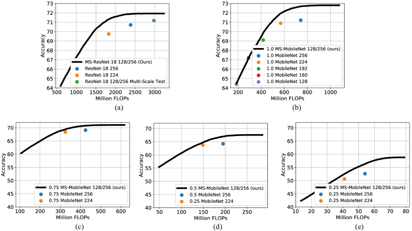
Since different thresholds lead to different computation costs and accuracies, we can achieve a speed-accuracy trade-off by varying the threshold values. We illustrate the relationship by enumerating multiple thresholds in Figure 5 for MS-ResNet-18 and MS-MobileNet (the black curve). The baseline approaches (colored dots) are also shown in the figure. We can easily observe the advantages of the MSNet over the baselines.

5 Conclusions

In this paper, we have presented a novel high frequency residual learning framework that decouples the learning of low frequency feature and high frequency feature. We demonstrate that computations can be saved by using a low resolution network to approximate the process of learning low frequency features. We have also proposed a classifier calibration module which can dynamically allocate computation resources during inference and lead to a better speed and accuracy trade-off. In our future work, we will design more flexible high frequency residual networks that can take as input arbitrary size of images. We will also demonstrate the effectiveness of high frequency residual learning in other recognition task, e.g. object detection and semantic segmentation, in the future.

Acknowledgements.

Bowen Cheng and Thomas Huang are in part supported by IBM-Illinois Center for Cognitive Computing Systems Research (C3SR) - a research collaboration as part of the IBM AI Horizons Network. The authors thank Bin Xiao for helpful discussions.

References

- [Bolukbasi et al.(2017)Bolukbasi, Wang, Dekel, and Saligrama] Tolga Bolukbasi, Joseph Wang, Ofer Dekel, and Venkatesh Saligrama. Adaptive neural networks for efficient inference. ICML, 2017.
- [Bourdev and Brandt(2005)] Lubomir Bourdev and Jonathan Brandt. Robust object detection via soft cascade. In IEEE CVPR, volume 2, pages 236–243. IEEE, 2005.
- [Chen et al.(2017a)Chen, Papandreou, Schroff, and Adam] Liang-Chieh Chen, George Papandreou, Florian Schroff, and Hartwig Adam. Rethinking atrous convolution for semantic image segmentation. arXiv preprint arXiv:1706.05587, 2017a.
- [Chen et al.(2018a)Chen, Papandreou, Kokkinos, Murphy, and Yuille] Liang-Chieh Chen, George Papandreou, Iasonas Kokkinos, Kevin Murphy, and Alan L Yuille. Deeplab: Semantic image segmentation with deep convolutional nets, atrous convolution, and fully connected crfs. IEEE TPAMI, 40(4):834–848, 2018a.
- [Chen et al.(2018b)Chen, Zhu, Papandreou, Schroff, and Adam] Liang-Chieh Chen, Yukun Zhu, George Papandreou, Florian Schroff, and Hartwig Adam. Encoder-decoder with atrous separable convolution for semantic image segmentation. In ECCV, 2018b.
- [Chen et al.(2017b)Chen, Li, Xiao, Jin, Yan, and Feng] Yunpeng Chen, Jianan Li, Huaxin Xiao, Xiaojie Jin, Shuicheng Yan, and Jiashi Feng. Dual path networks. In NIPS, pages 4470–4478, 2017b.
- [Cheng et al.(2017)Cheng, Wang, Zhang, Li, Liu, Yang, Huang, and Huang] Bowen Cheng, Zhangyang Wang, Zhaobin Zhang, Zhu Li, Ding Liu, Jianchao Yang, Shuai Huang, and Thomas S Huang. Robust emotion recognition from low quality and low bit rate video: A deep learning approach. In 2017 Seventh International Conference on Affective Computing and Intelligent Interaction (ACII), pages 65–70. IEEE, 2017.
- [Cheng et al.(2018a)Cheng, Liu, Wang, Zhang, and Huang] Bowen Cheng, Ding Liu, Zhangyang Wang, Haichao Zhang, and Thomas S Huang. Visual recognition in very low-quality settings: Delving into the power of pre-training. In Thirty-Second AAAI Conference on Artificial Intelligence, 2018a.
- [Cheng et al.(2018b)Cheng, Wei, Shi, Chang, Xiong, and Huang] Bowen Cheng, Yunchao Wei, Honghui Shi, Shiyu Chang, Jinjun Xiong, and Thomas S Huang. Revisiting pre-training: An efficient training method for image classification. arXiv preprint arXiv:1811.09347, 2018b.
- [Cheng et al.(2018c)Cheng, Wei, Shi, Feris, Xiong, and Huang] Bowen Cheng, Yunchao Wei, Honghui Shi, Rogerio Feris, Jinjun Xiong, and Thomas Huang. Decoupled classification refinement: Hard false positive suppression for object detection. arXiv preprint arXiv:1810.04002, 2018c.
- [Cheng et al.(2018d)Cheng, Wei, Shi, Feris, Xiong, and Huang] Bowen Cheng, Yunchao Wei, Honghui Shi, Rogerio Feris, Jinjun Xiong, and Thomas Huang. Revisiting rcnn: On awakening the classification power of faster rcnn. In ECCV, 2018d.
- [Cheng et al.(2018e)Cheng, Xiao, Guo, Hu, Wang, and Zhang] Bowen Cheng, Rong Xiao, Yandong Guo, Yuxiao Hu, Jianfeng Wang, and Lei Zhang. Revisit multinomial logistic regression in deep learning: Data dependent model initialization for image recognition. arXiv preprint arXiv:1809.06131, 2018e.
- [Chollet(2016)] François Chollet. Xception: Deep learning with depthwise separable convolutions. arXiv preprint, 2016.
- [Deng et al.(2009)Deng, Dong, Socher, Li, Li, and Fei-Fei] Jia Deng, Wei Dong, Richard Socher, Li-Jia Li, Kai Li, and Li Fei-Fei. Imagenet: A large-scale hierarchical image database. In IEEE CVPR, pages 248–255. IEEE, 2009.
- [Freund and Schapire(1997)] Yoav Freund and Robert E Schapire. A decision-theoretic generalization of on-line learning and an application to boosting. Journal of computer and system sciences, 55(1):119–139, 1997.
- [Girshick(2015)] Ross Girshick. Fast r-cnn. In IEEE ICCV, pages 1440–1448. IEEE, 2015.
- [Girshick et al.(2014)Girshick, Donahue, Darrell, and Malik] Ross Girshick, Jeff Donahue, Trevor Darrell, and Jitendra Malik. Rich feature hierarchies for accurate object detection and semantic segmentation. In IEEE CVPR, pages 580–587, 2014.
- [He et al.(2016)He, Zhang, Ren, and Sun] Kaiming He, Xiangyu Zhang, Shaoqing Ren, and Jian Sun. Deep residual learning for image recognition. In IEEE CVPR, pages 770–778, 2016.
- [Hinton et al.(2015)Hinton, Vinyals, and Dean] Geoffrey Hinton, Oriol Vinyals, and Jeff Dean. Distilling the knowledge in a neural network. arXiv preprint arXiv:1503.02531, 2015.
- [Howard et al.(2017)Howard, Zhu, Chen, Kalenichenko, Wang, Weyand, Andreetto, and Adam] Andrew G Howard, Menglong Zhu, Bo Chen, Dmitry Kalenichenko, Weijun Wang, Tobias Weyand, Marco Andreetto, and Hartwig Adam. Mobilenets: Efficient convolutional neural networks for mobile vision applications. arXiv preprint arXiv:1704.04861, 2017.
- [Huang et al.(2017)Huang, Liu, Weinberger, and van der Maaten] Gao Huang, Zhuang Liu, Kilian Q Weinberger, and Laurens van der Maaten. Densely connected convolutional networks. In IEEE CVPR, volume 1, page 3, 2017.
- [Huang et al.(2018)Huang, Chen, Li, Wu, van der Maaten, and Weinberger] Gao Huang, Danlu Chen, Tianhong Li, Felix Wu, Laurens van der Maaten, and Kilian Q Weinberger. Multi-scale dense networks for resource efficient image classification. ICLR, 2018.
- [Iandola et al.(2016)Iandola, Han, Moskewicz, Ashraf, Dally, and Keutzer] Forrest N Iandola, Song Han, Matthew W Moskewicz, Khalid Ashraf, William J Dally, and Kurt Keutzer. Squeezenet: Alexnet-level accuracy with 50x fewer parameters and< 0.5 mb model size. arXiv preprint arXiv:1602.07360, 2016.
- [Krizhevsky et al.(2012)Krizhevsky, Sutskever, and Hinton] Alex Krizhevsky, Ilya Sutskever, and Geoffrey E Hinton. Imagenet classification with deep convolutional neural networks. In NIPS, pages 1097–1105, 2012.
- [Liu et al.(2017)Liu, Cheng, Wang, Zhang, and Huang] Ding Liu, Bowen Cheng, Zhangyang Wang, Haichao Zhang, and Thomas S Huang. Enhance visual recognition under adverse conditions via deep networks. arXiv preprint arXiv:1712.07732, 2017.
- [Long et al.(2015)Long, Shelhamer, and Darrell] Jonathan Long, Evan Shelhamer, and Trevor Darrell. Fully convolutional networks for semantic segmentation. In IEEE CVPR, pages 3431–3440, 2015.
- [Newell et al.(2016)Newell, Yang, and Deng] Alejandro Newell, Kaiyu Yang, and Jia Deng. Stacked hourglass networks for human pose estimation. In European Conference on Computer Vision, pages 483–499. Springer, 2016.
- [Pedersoli et al.(2015)Pedersoli, Vedaldi, Gonzalez, and Roca] Marco Pedersoli, Andrea Vedaldi, Jordi Gonzalez, and Xavier Roca. A coarse-to-fine approach for fast deformable object detection. Pattern Recognition, 48(5):1844–1853, 2015.
- [Polino et al.(2018)Polino, Pascanu, and Alistarh] Antonio Polino, Razvan Pascanu, and Dan Alistarh. Model compression via distillation and quantization. arXiv preprint arXiv:1802.05668, 2018.
- [Rastegari et al.(2016)Rastegari, Ordonez, Redmon, and Farhadi] Mohammad Rastegari, Vicente Ordonez, Joseph Redmon, and Ali Farhadi. Xnor-net: Imagenet classification using binary convolutional neural networks. In ECCV, pages 525–542. Springer, 2016.
- [Real et al.(2018)Real, Aggarwal, Huang, and Le] Esteban Real, Alok Aggarwal, Yanping Huang, and Quoc V Le. Regularized evolution for image classifier architecture search. 2018.
- [Ren et al.(2015)Ren, He, Girshick, and Sun] Shaoqing Ren, Kaiming He, Ross Girshick, and Jian Sun. Faster r-cnn: Towards real-time object detection with region proposal networks. In NIPS, pages 91–99, 2015.
- [Romero et al.(2014)Romero, Ballas, Kahou, Chassang, Gatta, and Bengio] Adriana Romero, Nicolas Ballas, Samira Ebrahimi Kahou, Antoine Chassang, Carlo Gatta, and Yoshua Bengio. Fitnets: Hints for thin deep nets. arXiv preprint arXiv:1412.6550, 2014.
- [Sandler et al.(2018)Sandler, Howard, Zhu, Zhmoginov, and Chen] Mark Sandler, Andrew Howard, Menglong Zhu, Andrey Zhmoginov, and Liang-Chieh Chen. Inverted residuals and linear bottlenecks: Mobile networks for classification, detection and segmentation. arXiv preprint arXiv:1801.04381, 2018.
- [Saxena and Verbeek(2016)] Shreyas Saxena and Jakob Verbeek. Convolutional neural fabrics. In Advances in Neural Information Processing Systems, pages 4053–4061, 2016.
- [Simonyan and Zisserman(2014)] Karen Simonyan and Andrew Zisserman. Very deep convolutional networks for large-scale image recognition. arXiv preprint arXiv:1409.1556, 2014.
- [Sun et al.(2019)Sun, Xiao, Liu, and Wang] Ke Sun, Bin Xiao, Dong Liu, and Jingdong Wang. Deep high-resolution representation learning for human pose estimation. arXiv preprint arXiv:1902.09212, 2019.
- [Szegedy et al.()Szegedy, Liu, Jia, Sermanet, Reed, Anguelov, Erhan, Vanhoucke, Rabinovich, Rick Chang, et al.] Christian Szegedy, Wei Liu, Yangqing Jia, Pierre Sermanet, Scott Reed, Dragomir Anguelov, Dumitru Erhan, Vincent Vanhoucke, Andrew Rabinovich, Jen-Hao Rick Chang, et al. Going deeper with convolutions. In IEEE CVPR.
- [Szegedy et al.(2017)Szegedy, Ioffe, Vanhoucke, and Alemi] Christian Szegedy, Sergey Ioffe, Vincent Vanhoucke, and Alexander A Alemi. Inception-v4, inception-resnet and the impact of residual connections on learning. In AAAI, volume 4, page 12, 2017.
- [Teerapittayanon et al.(2016)Teerapittayanon, McDanel, and Kung] Surat Teerapittayanon, Bradley McDanel, and HT Kung. Branchynet: Fast inference via early exiting from deep neural networks. In Pattern Recognition (ICPR), 2016 23rd International Conference on, pages 2464–2469. IEEE, 2016.
- [Viola and Jones(2004)] Paul Viola and Michael J Jones. Robust real-time face detection. IJCV, 57(2):137–154, 2004.
- [Wang et al.(2016)Wang, Chang, Yang, Liu, and Huang] Zhangyang Wang, Shiyu Chang, Yingzhen Yang, Ding Liu, and Thomas S Huang. Studying very low resolution recognition using deep networks. In Proceedings of the IEEE Conference on Computer Vision and Pattern Recognition, pages 4792–4800, 2016.
- [Wei et al.(2018)Wei, Shen, Cheng, Shi, Xiong, Feng, and Huang] Yunchao Wei, Zhiqiang Shen, Bowen Cheng, Honghui Shi, Jinjun Xiong, Jiashi Feng, and Thomas Huang. Ts2c: Tight box mining with surrounding segmentation context for weakly supervised object detection. In ECCV, 2018.
- [Xie et al.(2018)Xie, Wang, Zhang, Lai, Hong, and Qi] Guotian Xie, Jingdong Wang, Ting Zhang, Jianhuang Lai, Richang Hong, and Guo-Jun Qi. Interleaved structured sparse convolutional neural networks. In Proceedings of the IEEE Conference on Computer Vision and Pattern Recognition, pages 8847–8856, 2018.
- [Xie et al.(2017)Xie, Girshick, Dollár, Tu, and He] Saining Xie, Ross Girshick, Piotr Dollár, Zhuowen Tu, and Kaiming He. Aggregated residual transformations for deep neural networks. In IEEE CVPR, pages 5987–5995. IEEE, 2017.
- [Yang et al.(2017)Yang, Li, Ouyang, Li, and Wang] Wei Yang, Shuang Li, Wanli Ouyang, Hongsheng Li, and Xiaogang Wang. Learning feature pyramids for human pose estimation. In Proceedings of the IEEE International Conference on Computer Vision, pages 1281–1290, 2017.
- [Yu and Huang(2019)] Jiahui Yu and Thomas Huang. Universally slimmable networks and improved training techniques. arXiv preprint arXiv:1903.05134, 2019.
- [Yu et al.(2018)Yu, Yang, Xu, Yang, and Huang] Jiahui Yu, Linjie Yang, Ning Xu, Jianchao Yang, and Thomas Huang. Slimmable neural networks. arXiv preprint arXiv:1812.08928, 2018.
- [Zhang et al.(2007)Zhang, Zelinsky, and Samaras] Wei Zhang, Gregory Zelinsky, and Dimitris Samaras. Real-time accurate object detection using multiple resolutions. In 2007 IEEE 11th International Conference on Computer Vision, pages 1–8. IEEE, 2007.
- [Zhang et al.(2017)Zhang, Zhou, Lin, and Sun] Xiangyu Zhang, Xinyu Zhou, Mengxiao Lin, and Jian Sun. Shufflenet: An extremely efficient convolutional neural network for mobile devices. arXiv preprint arXiv:1707.01083, 2017.
- [Zhao et al.(2017)Zhao, Shi, Qi, Wang, and Jia] Hengshuang Zhao, Jianping Shi, Xiaojuan Qi, Xiaogang Wang, and Jiaya Jia. Pyramid scene parsing network. In Proceedings of the IEEE conference on computer vision and pattern recognition, pages 2881–2890, 2017.
- [Zoph et al.(2018)Zoph, Vasudevan, Shlens, and Le] Barret Zoph, Vijay Vasudevan, Jonathon Shlens, and Quoc V Le. Learning transferable architectures for scalable image recognition. In IEEE CVPR, 2018.