Field-induced dissociation of two-dimensional excitons in transition-metal dichalcogenides

Abstract

Generation of photocurrents in semiconducting materials requires dissociation of excitons into free charge carriers. While thermal agitation is sufficient to induce dissociation in most bulk materials, an additional push is required to induce efficient dissociation of the strongly bound excitons in monolayer transition-metal dichalcogenides (TMDs). Recently, static in-plane electric fields have proven to be a promising candidate. In the present paper, we introduce a numerical procedure, based on exterior complex scaling, capable of computing field-induced exciton dissociation rates for a wider range of field strengths than previously reported in literature. We present both Stark shifts and dissociation rates for excitons in various TMDs calculated within the Mott-Wannier model. Here, we find that the field induced dissociation rate is strongly dependent on the dielectric screening environment. Furthermore, applying weak-field asymptotic theory (WFAT) to the Keldysh potential, we are able to derive an analytical expression for exciton dissociation rates in the weak-field region.

I Introduction

Interest in two-dimensional transition-metal dichalcogenide (TMD) semiconductors has increased substantially in recent years due to their exceptional electronic and optical properties. They have a wide range of applications, including photodetectors Wang et al. (2015); Lopez-Sanchez et al. (2013); Yin et al. (2012), light-emitting diodes Withers et al. (2015), solar cells Lopez-Sanchez et al. (2014); Bernardi et al. (2013), and energy storage devices Du et al. (2010); Chhowalla et al. (2013); Soon and Loh (2007), to name a few. One of the most important implications of the reduced screening in two-dimensional TMDs is the comparatively large exciton binding energy Ramasubramaniam (2012); Latini et al. (2015); Berkelbach et al. (2013); Pedersen et al. (2016a). Such excitons may significantly reduce the efficiency of solar cells and photodetectors, as these devices require the dissociation of excitons into free charge carriers to generate an electrical current. Excitons in bulk semiconductors will usually dissociate by thermal agitation alone due to their low binding energies. This is not the case for their two-dimensional counterparts, however, and it is therefore of great interest to obtain efficient methods of inducing exciton dissociation in TMD monolayers. Dissociation induced by in-plane static electric fields has gained attraction lately. For instance, dissociation rates for two-dimensional excitons in MoS₂ and $h$BN/MoS₂ were theoretically investigated in Ref. Haastrup et al. (2016) and for various bulk TMDs in Pedersen et al. (2016a).
Recently, the first systematic experimental study of field-induced dissociation of two-dimensional excitons in monolayer WSe₂ encapsulated by $h$BN was carried out Massicotte et al. (2018). It was found that the limiting factor in generating photocurrents when a weak in-plane field was present was the dissociation rate of electron-hole pairs. That work also showed that the photocurrent generated in fields weaker than $15\,\mathrm{V/\mu m}$ was accurately predicted by the Mott-Wannier model Wannier (1937); Lederman and Dow (1976). Nevertheless, these weak-field dissociation rates proved troublesome to obtain numerically Massicotte et al. (2018), and they were therefore extrapolated by fitting to the rate of a two-dimensional hydrogen atom Pedersen et al. (2016b). In the present paper, we introduce a numerical method capable of computing exciton dissociation rates for significantly weaker fields with no compromise on the accuracy for stronger fields. It is based on the complex scaling approach Balslev and Combes (1971); Aguilar and Combes (1971) that was used in Refs. Haastrup et al. (2016) and Massicotte et al. (2018), but, rather than rotating the entire spatial region into the complex plane, we rotate the radial coordinate only in an exterior region $r>R$. For sufficiently weak fields, we show that the rates can be obtained analytically based on the recently developed weak-field asymptotic theory (WFAT) Tolstikhin et al. (2011), which greatly simplifies their calculation. Furthermore, we show that the weak-field ionization rate of two-dimensional hydrogen is a special case of a more general formula for dissociation of a two-dimensional two-particle system.

II TMD Exciton in Electrostatic Field

Throughout the present paper, excitons will be modeled as electron-hole pairs described by the two-dimensional Wannier equation Wannier (1937); Lederman and Dow (1976), which reads (atomic units are used throughout)

$$\left[-\frac{1}{2\mu}\nabla^{2}-w\left(\kappa\boldsymbol{r}\right)\right]\psi\left(\boldsymbol{r}\right)=E\psi\left(\boldsymbol{r}\right)\thinspace,$$ (1)

where $\mu$ is the reduced exciton mass, $\boldsymbol{r}=\boldsymbol{r}_{e}-\boldsymbol{r}_{h}$ is the relative in-plane coordinate of the electron-hole pair, $\kappa=\left(\kappa_{a}+\kappa_{b}\right)/2$ is the average dielectric constant of the materials above and beneath the TMD sheet, and $w$ is a screened Coulomb attraction. It is well known that screening in two-dimensional semiconductors, such as TMDs, is inherently nonlocal Cudazzo et al. (2010); Keldysh (1979), i.e. momentum-dependent, and can be approximated by the linearized form $\epsilon\left(\boldsymbol{q}\right)=\kappa+r_{0}q$ , where $\boldsymbol{q}$ is the wave vector and the so-called screening length $r_{0}$ can be related to the polarizability of the sheet Cudazzo et al. (2010). The interaction $w$ may then be obtained as the inverse Fourier transform of $2\pi\left[\epsilon\left(\boldsymbol{q}\right)q\right]^{-1}$, where $2\pi/q$ is the 2D Fourier transform of $1/r$. The resulting interaction is given by the Keldysh Keldysh (1979); Trolle et al. (2017) form

$$w\left(\boldsymbol{r}\right)=\frac{\pi}{2r_{0}}\left[\mathrm{H}_{0}\left(\frac{r}{r_{0}}\right)-Y_{0}\left(\frac{r}{r_{0}}\right)\right]\thinspace,$$ (2)

where $\mathrm{H}_{0}$ is the zeroth order Struve function and $Y_{0}$ is the zeroth order Bessel function of the second kind Abramowitz (1974).

When an in-plane electrostatic field is applied to the exciton, Eq. 1 is modified to include a perturbation term

$$\left[-\frac{1}{2\mu}\nabla^{2}-w\left(\kappa\boldsymbol{r}\right)+\boldsymbol{\varepsilon}\cdot\boldsymbol{r}\right]\psi\left(\boldsymbol{r}\right)=E\psi\left(\boldsymbol{r}\right)\thinspace.$$ (3)

In the present paper, we will restrict ourselves to electric fields pointing along the $x$-axis, i.e., $\boldsymbol{\varepsilon}=\varepsilon\boldsymbol{e}_{x}$. As is evident, the form of Eq. 3 is the same as that of the two-dimensional hydrogen atom in a static electric field Pedersen et al. (2016b), albeit with a different potential. It should therefore come as no surprise that excitons perturbed by an electrostatic field will eventually dissociate. An important distinction, however, is that the excitons will recombine if they are not dissociated Koch et al. (2006); Massicotte et al. (2018). This field-free recombination rate is in competition with the field-induced dissociation. For practical applications, recombination Palummo et al. (2015); Wang et al. (2016); Poellmann et al. (2015) and other forms of exciton decay (such as defect-assisted recombination Shi et al. (2013) and exciton-exciton annihilation Sun et al. (2014)) that do not yield free charge carriers, are often undesired.

The field-induced dissociation rate $\Gamma$ is connected to the non-vanishing imaginary part of the energy eigenvalue in the presence of an electric field by the relation $\Gamma=-2\mathrm{Im}\,E$ Haastrup et al. (2016); Pedersen et al. (2016a); Massicotte et al. (2018); Pedersen et al. (2016b). The desired eigenvalues are therefore unobtainable through conventional Hermitian methods. Rather, one should solve Eq. 3 subject to regularity and outgoing boundary conditions Tolstikhin et al. (2011); Siegert (1939). This is a nontrivial task in all but the simplest cases, and in practice, one usually computes the resonance energies by complex scaling the Hamiltonian Balslev and Combes (1971); Aguilar and Combes (1971).

III Exciton Dissociation

Figure 1: Sketch of the two-dimensional exciton in the $xy$-plane with the radial coordinate rotated into the complex plane by an angle of $\phi$ for $r>R$.

In its simplest form, complex scaling corresponds to rotating the radial coordinate into the complex plane uniformly Balslev and Combes (1971); Aguilar and Combes (1971) $r\to\exp\left(i\phi\right)r$ , where $\phi$ is a fixed real-valued angle (note that if $\phi$ is chosen complex the coordinate will simply be stretched as well as rotated). This transformation, referred to as uniform complex scaling (UCS), turns the outgoing waves mentioned above into exponentially decaying waves, provided that $\phi$ is chosen large enough McCurdy et al. (2004). Thus, the complex scaled resonance wave functions are square integrable, and the resonance energies can be obtained by solving Eq. 3 with the scaled operator and the boundary condition $\psi\left(r\to\infty\right)=0$. This approach has been used to obtain the dissociation rates of two-dimensional TMD excitons in Refs. Haastrup et al. (2016) and Massicotte et al. (2018). Nevertheless, as was discussed briefly in Ref. Massicotte et al. (2018), numerical difficulties arise when the electric field becomes sufficiently weak. This is because the important region for weak fields is sufficiently far from the origin that the uniformly complex scaled resonance wave function has (numerically) vanished prior to reaching this region. By utilizing the so-called exterior complex scaling (ECS) approach Simon (1979); McCurdy et al. (2004, 1991); Rescigno and McCurdy (2000), combined with a finite element (FE) representation of the wave function, we are able to compute dissociation rates for significantly weaker fields, as we now demonstrate.

As the name suggests, ECS transforms the radial coordinate outside a scaling radius $R$

$$r\to\begin{cases}r\quad&\mathrm{for}\,\,r<R\\ R+\left(r-R\right)e^{i\phi}\quad&\mathrm{for}\,\,r>R\thinspace,\end{cases}$$ (4)

where $\phi$ is the angle of rotation, as illustrated in Fig. 1. The partitioning of the radial coordinate is efficiently dealt with by an FE basis representation, the details of which can be found in App. A. The Stark shift and dissociation rate as functions of in-plane field strength for four important materials in various dielectric environments are shown in Fig. 2. The screening lengths and reduced masses used in the calculations are obtained from Ref. Olsen et al. (2016). As is evident, the dissociation rate increases rapidly with increasing field strength. The rates can also be seen to be strongly dependent on the screening environment, which is to be expected as increased screening leads to reduced binding energies. It is therefore possible to tune the dissociation rates of the TMDs as desired within a certain range. For example, encapsulating the TMDs in $h$BN (with $\kappa=4.9$ Latini et al. (2015)) increases the dissociation rates by several orders of magnitude compared to their free-space counterparts. Rates for MoS₂, MoS₂/$h$BN, and $h$BN/MoS₂/$h$BN were presented in Ref. Haastrup et al. (2016) for fields stronger than $50\,\mathrm{V/\mu m}$. However, the experimental study of $h$BN/WSe₂/$h$BN in Ref. Massicotte et al. (2018) suggests that exciton dissociation rates are the limiting factor in generation of photocurrents for applied fields weaker than $15\,\mathrm{V/\mu m}$ in this material. For stronger fields, the photocurrent measurements deviate from the field-induced rates predicted by the Wannier model, and other limitations dominate Massicotte et al. (2018). We expect to see the same effect for the other TMDs, and we furthermore expect this threshold field to increase as the screening is reduced.
In weak fields, the Stark shifts in Fig. 2 can be seen to vary approximately as $\varepsilon^{2}$, in agreement with the lowest order perturbation theory expansion of the energy $E\approx E_{0}-\frac{1}{2}\alpha\varepsilon^{2}$ , where $E_{0}$ is the unperturbed ground-state energy and $\alpha$ is the exciton polarizability. The shape of the shift is in agreement with those observed for similar systems; the energy initially decreases rapidly with field strength and then levels off as the field strength increases Pedersen et al. (2016b). A more detailed analysis of the shift in the weak-field region will be made in Sec. V.

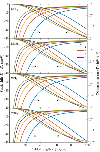
Figure 2: Exciton Stark shift and dissociation rate for four important materials in various dielectric environments.

IV Weak-field Asymptotic Theory

Even with our improved numerical procedure, the dissociation rates for extremely weak fields are unobtainable. In fact, any numerical procedure with finite-precision arithmetic fails for sufficiently weak fields, when the ratio $\Gamma/\left|E_{0}\right|$ approaches the round-off error Trinh et al. (2013); Batishchev et al. (2010). Fortunately, with the recent development of weak-field asymptotic theory (WFAT) Tolstikhin et al. (2011), we are able to take advantage of the simple asymptotic form of the Keldysh potential and calculate the weak-field dissociation rates analytically. To this end, we first simplify Eq. 3 by introducing the scaling relations

$$\tilde{r}_{0}=\frac{\mu}{\kappa^{2}}r_{0}\thinspace,\quad\tilde{\boldsymbol{r}}=\frac{\mu}{\kappa}\boldsymbol{r},\quad\mathrm{and}\quad\tilde{\boldsymbol{\varepsilon}}=\frac{\kappa^{3}}{\mu^{2}}\boldsymbol{\varepsilon}\thinspace,$$ (5)

which lead to

$$E\left(\mu,\kappa,r_{0},\varepsilon\right)=\frac{\mu}{\kappa^{2}}E\left(1,1,\tilde{r}_{0},\tilde{\varepsilon}\right)\thinspace.$$ (6)

Thus, the only nontrivial parameters are $\tilde{r}_{0}$ and $\tilde{\varepsilon}$ , and the analysis in the following will therefore be restricted to the simplified problem

$$\left[-\frac{1}{2}\nabla^{2}-w\left(\boldsymbol{r}\right)+\boldsymbol{\varepsilon}\cdot\boldsymbol{r}\right]\psi\left(\boldsymbol{r}\right)=E\psi\left(\boldsymbol{r}\right)\thinspace,$$ (7)

from which Stark shifts and dissociation rates can be obtained using Eq. 6. Note that in order to simplify the notation the tilde has been omitted in Eq. 7 as well as in the following. Therefore, unless explicitly stated otherwise, $r$, $r_{0}$, $\varepsilon$, and $E$ in the following refer to the scaled parameters.

The potential in Eq. 7 has the large-$r$ behavior Abramowitz (1974)

$$w\left(\boldsymbol{r}\right)=\frac{1}{r}+O\left(\frac{r_{0}^{2}}{r^{3}}\right)\thinspace,$$ (8)

which has the form required to use WFAT. A leading order expression for the weak-field dissociation rate was derived for a three-dimensional system in Ref. Tolstikhin et al. (2011) and extended to first order in $\varepsilon$ in Ref. Trinh et al. (2013). We shall only consider the leading order approximation here. By modifying the approach in Ref. Tolstikhin et al. (2011) to two dimensions, we find that the weak-field dissociation rate for the ground-state of Eq. 7 is given by

$$\Gamma\approx\left|g_{0}\right|^{2}W_{0}\left(\varepsilon\right)\thinspace,$$ (9)

with the asymptotic coefficient and field factor Madsen et al. (2012, 2013) given by

$$g_{0}=\lim_{v\to\infty}v^{1/2-1/k}e^{kv/2}\\ \times\int_{0}^{\infty}\varphi_{0}\left(u\right)\psi_{0}\left(\frac{u+v}{2}\right)\frac{1}{\sqrt{u}}du$$ (10)

and

$$W_{0}\left(\varepsilon\right)=k\left(\frac{4k^{2}}{\varepsilon}\right)^{2/k-1/2}\exp\left(-\frac{2k^{3}}{3\varepsilon}\right)\thinspace,$$ (11)

respectively. Here, $k=\sqrt{-2E_{0}}$, and $u$ and $v$ are the parabolic cylindrical coordinates defined by

$$u=r+x\thinspace,\quad u\in\left[0,\infty\right)$$ (12)

$$v=r-x\thinspace,\quad v\in\left[0,\infty\right)\thinspace.$$ (13)

The functions appearing in Eq. 10 are the unperturbed ground state $\psi_{0}$ and

$$\varphi_{n}\left(u\right)=\left[\frac{\sqrt{k}n!}{\left(n-1/2\right)!}\right]^{1/2}L_{n}^{\left(-1/2\right)}\left(ku\right)e^{-ku/2}\thinspace,$$ (14)

with $L_{n}^{\left(\alpha\right)}\left(x\right)$ a generalized Laguerre polynomial Abramowitz (1974). To obtain the weak field dissociation rate from Eq. 9, one therefore needs the unperturbed binding energy $E_{0}$ and the asymptotic coefficient $g_{0}$ of the simplified problem. Once they have been obtained, the physical weak-field dissociation rate for arbitrary monolayer TMDs can be obtained by scaling back to the original units, cf. Eq. 6,

$$\Gamma\left(\mu,\kappa,r_{0},\varepsilon\right)=\frac{\mu}{\kappa^{2}}\Gamma\left(1,1,\tilde{r}_{0},\tilde{\varepsilon}\right)\thinspace.$$ (15)

We now turn to computing the asymptotic coefficient $g_{0}$.

IV.1 Computing the asymptotic coefficient

Table 1: Binding energy $E_{0}\left(1,1,\tilde{r}_{0}\right)$ and asymptotic coefficient $g_{0}$ of the simplified problem for four important materials in different dielectric environments.

	MoS2			MoSe2			WS2			WSe2
$\kappa$	$E_{0}$	$g_{0}$		$E_{0}$	$g_{0}$		$E_{0}$	$g_{0}$		$E_{0}$	$g_{0}$
$1$	$0.0714$	$0.00098$		$0.0659$	$0.00057$		$0.0921$	$0.0044$		$0.0801$	$0.0020$
$2$	$0.1907$	$0.0889$		$0.1773$	$0.0707$		$0.2392$	$0.1671$		$0.2113$	$0.1200$
$3$	$0.3200$	$0.3210$		$0.2995$	$0.2805$		$0.3928$	$0.4650$		$0.3512$	$0.3829$
$4$	$0.4474$	$0.5695$		$0.4210$	$0.5195$		$0.5392$	$0.7323$		$0.4870$	$0.6420$
$5$	$0.5680$	$0.7796$		$0.5370$	$0.729$		$0.6740$	$0.9380$		$0.6142$	$0.8515$

Finding $g_{0}$ given by Eq. 10 requires an accurate representation of the wave function for large $v$. Note that a traditional basis expansion (e.g. a Gaussian basis) is generally not accurate enough, as only the most slowly decaying functions will contribute in this region. This problem was partially circumvented in Ref. Madsen et al. (2013) by using a Guassian basis with optimized exponents. Here, we will implement Numerov’s finite difference scheme, which can accurately and efficiently construct the unperturbed wave function in the asymptotic region. The technical details can be found in App. B. As a preliminary, it is convenient to relate $g_{0}$ to the radial wave function. The ground state of a potential with cylindrical symmetry satisfies

$$\psi_{0}\left(r\right)\sim C_{0}r^{1/k-1/2}e^{-kr}\quad\mathrm{for}\,r\to\infty\thinspace,$$ (16)

where $C_{0}$ is a constant. Using Eq. 16 in Eq. 10 leads to the relation

$$g_{0}=\frac{2^{1/2-1/k}\pi^{1/4}C_{0}}{k^{1/4}}\thinspace.$$ (17)

The problem of finding $g_{0}$ has therefore been reduced to obtaining the asymptotic coefficient of the radial wave function. It can be found by taking the limit

$$C_{0}=\lim_{r\to\infty}\psi_{0}r^{1/2-1/k}e^{kr}.$$ (18)

Note that in the unscreened limit ($r_{0}\to 0$) $k=2$ and $\psi_{0}=2^{3/2}\pi^{-1/2}\exp\left[-\left(u+v\right)\right]$ Yang et al. (1991) which leads to $g_{0}=2^{5/4}\pi^{-1/4}$, and Eq. 9 is therefore in agreement with the expression found in Ref. Pedersen et al. (2016b) for the two-dimensional hydrogen atom. In practice, we find $C_{0}$ by fitting Eq. 18 to the asymptotic expansion

$$D\left(r\right)=\sum_{n=0}^{4}\frac{d_{n}}{r^{n}}\thinspace,$$ (19)

in a stable region (see App. B), as described in Ref. Madsen et al. (2013). The asymptotic coefficient $C_{0}$ is then obtained by taking the limit $\lim_{r\to\infty}D=d_{0}$.

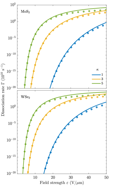
Figure 3: Exciton dissociation rates for MoS₂ (upper) and WSe₂ (lower) encapsulated by various dielectric media. The circles are the numerically exact results obtained by the method in App. A (same as those in Fig. 2). The solid lines correspond to the weak-field formula Eq. 9 with the parameters found in Tbl. 1.

The computational method above takes advantage of the fact that a high-order finite-difference scheme is able to accurately reproduce the wave function for large $r$. Recently, however, integral representations for the asymptotic coefficient that are insensitive to the wave function tail have been derived for a three-dimensional system Dnestryan and Tolstikhin (2016); Madsen et al. (2017). This suggests that one may get away with using a sufficiently accurate representation of the wave function only in an interior region. We shall use the integral equations as a check to ensure the accuracy of the scheme presented above. To derive the corresponding equation for our two-dimensional system we introduce the reference function $\Omega$ as a solution to

$$\left[-\frac{1}{2}\nabla^{2}-\frac{1}{r}+\frac{k^{2}}{2}\right]\Omega_{n}\left(r\right)=0\thinspace.$$ (20)

The relevant function for the asymptotic coefficient of the ground state is

$$\Omega_{0}\left(r\right)=-2^{\frac{1}{k}+\frac{1}{2}}k^{\frac{1}{k}-\frac{1}{2}}\Gamma\left(\frac{1}{2}-\frac{1}{k}\right)\\ \times\,e^{-kr}M\left(\frac{1}{2}-\frac{1}{k};1;2kr\right)\thinspace,$$ (21)

where $\,M$ is a confluent hypergeometric function Abramowitz (1974). If the exciton energy coincides with one of the energies of the two-dimensional hydrogen atom

$$E_{n}^{\left(\mathrm{hydr.}\right)}=\frac{1}{2\left(n-1/2\right)^{2}}\thinspace,$$ (22)

where $n=1,2,...$ Yang et al. (1991), the confluent hypergeometric function in Eq. 21 reduces to a polynomial of finite degree and $\Omega_{0}$ will vanish as $r$ tends to infinity. In practical calculations, this is hardly ever the case and the reference function will therefore be exponentially increasing (see Ref. Dnestryan et al. (2018) for a discussion of the case where $E_{0}\approx E_{n}^{\left(\mathrm{hydr.}\right)}$)

$$\Omega\left(r\right)\sim-k^{-1}r^{-1/2-1/k}e^{kr}\quad\mathrm{for}\,r\to\infty\thinspace.$$ (23)

Integrating by parts and using Eqs. 16 and 23 when $r$ tends to infinity, we find

$$C_{0}=\int_{0}^{\infty}\Omega_{0}\left(r\right)\left[\frac{1}{2}\nabla^{2}+\frac{1}{r}-\frac{k^{2}}{2}\right]\psi_{0}\left(r\right)rdr\thinspace,$$ (24)

which, using Eq. 7 with $\varepsilon=0$, can be reduced to

$$C_{0}=\int_{0}^{\infty}\Omega_{0}\left(r\right)\left[\frac{1}{r}-w_{s}\left(r\right)\right]\psi_{0}\left(r\right)rdr\thinspace.$$ (25)

The integrand in Eq. 25 is a product of an exponentially increasing function $\Omega_{0}$ and an exponentially decreasing function $\psi_{0}$. Such an integral need not be convergent. Nevertheless, as is evident from the large-$r$ behavior of these functions (see Eqs. 16 and 23), the exponential terms cancel for $r$ tending to infinity, resulting in the integrand tending to zero sufficiently quickly for the integral to converge. We have checked that Eqs. 18 and 25 agree when using the numerically exact wave function. The asymptotic coefficients and binding energies of the simplified Wannier problem for four important materials are presented in Tbl. 1. Note that these binding energies increase with $\kappa$. This is because the binding energies of the simplified problem increase when $\tilde{r}_{0}$ decreases and $\tilde{r}_{0}$ is proportional to $\kappa^{-2}$. In Fig. 3, we compare the dissociation rates for excitons in MoS₂ and WSe₂ given by the weak-field formula Eq. 9 to the numerically exact dissociation rates. As can be seen, the agreement between the weak-field and the fully numerical results is reasonable for fields lower than $50\mathrm{V/\mu m}$ and improves as the field strength decreases. For $\varepsilon\lesssim\kappa^{-1/2}\,20\,\mathrm{V/\mu m}$ the agreement in Fig. 3 becomes excellent.

V Stark Shift

Table 2: Exciton polarizability $\alpha$ for various TMDs in different dielectric environments in units of $10^{-18}\mathrm{eV}\left(\mathrm{m/V}\right)^{2}$ calculated from Eq. 27 with $\psi_{0}$ and $\psi_{1}$ expanded in an FE basis with a spacing of $1$ a.u..

	MoS2		MoSe2		WS2		WSe2
$\kappa$	$\alpha$		$\alpha$		$\alpha$		$\alpha$
$1$	$4.59$		$6.24$		$5.04$		$6.24$
$2$	$6.31$		$8.46$		$7.30$		$8.78$
$3$	$8.48$		$11.22$		$10.25$		$12.02$
$4$	$11.18$		$14.63$		$14.09$		$16.14$
$5$	$14.54$		$18.81$		$19.00$		$21.32$

Applying perturbation theory to the ground state of a system with cylindrical symmetry leads to the well known result

$$E=E_{0}-\frac{1}{2}\alpha\varepsilon^{2}+O\left(\varepsilon^{4}\right)\thinspace,$$ (26)

where $\alpha$ is the static polarizability. A shortcoming of perturbation theory is that it predicts the energy as a function of field strength to be purely real, which, as seen in the previous sections, is obviously not correct for a system where dissociation is possible. Nevertheless, the non-perturbative behavior of the resonance energy can be reproduced by utilizing the first few perturbation coefficients together with the hypergeometric resummation technique Mera et al. (2015). This approach was used in Ref. Pedersen et al. (2016b) with great success for low-dimensional hydrogen. In the present section, we wish to analyze to what degree the change in the real part of the resonance energy, i.e. the exciton Stark shift, can be predicted by standard second-order perturbation theory. To this end, we calculate the exciton polarizability given by

$$\alpha=-2\left<\psi_{0}\right|r\cos\theta\left|\psi_{1}\right>\thinspace,$$ (27)

where the first order correction $\psi_{1}$ is a solution to the Dalgarno-Lewis Dalgarno et al. (1955) equation

$$\left[-\frac{1}{2\mu}\nabla^{2}-w\left(\kappa\boldsymbol{r}\right)-E_{0}\right]\psi_{1}=-r\cos\theta\psi_{0}\thinspace,$$ (28)

and will therefore be of the form $\psi_{1}=\cos\theta f\left(r\right)$, where $f$ is a purely radial function. Expanding $\psi_{0}$ and $\psi_{1}$ in a finite element basis (without complex scaling), as described in App. A, Eq. 28 can be solved and the polarizability found (for alternative methods of finding the polarizability, see Ref. Pedersen (2016)). The exciton polarizability for various TMDs in different environments can be found in Tbl. 2, and Fig. 4 shows a comparison between the shift in the real part of the complex resonance energy and the perturbation series in Eq. 26. Evidently, a good agreement is found in the weak field region. Furthermore, excitons in environments with large dielectric screening begin to deviate from their second-order expansion for weaker fields than their free-space counterparts. This is to be expected, as the binding energies of excitons with heavily screened interactions are lower and the characteristic fields of these excitons are therefore weaker.

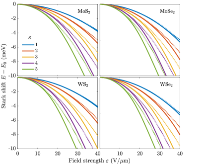
Figure 4: Exciton Stark shift for four important TMDs in various dielectric environments. The solid lines correspond to the real part of the resonance energy, while the dotted lines show to the shift predicted by perturbation theory $E-E_{0}\approx-\alpha\varepsilon^{2}/2$.

VI Summary

In the present work, electric field induced dissociation of TMD excitons has been investigated using both numerical and analytical approaches. The dissociation rates as functions of the in-plane field strength for excitons in monolayer MoS₂, MoSe₂, WS₂, and WSe₂ in various screening environments have been obtained. In particular, difficulties associated with dissociation rates in weak electric fields have been addressed and resolved. In this regard, an efficient numerical method capable of computing dissociation rates for a wide range of fields has been introduced. As the field becomes sufficiently weak, any numerical method with finite precision arithmetic breaks down, which calls for a different approach. We demonstrate that an analytical weak-field approximation is valid in this region, which makes the weak-field dissociation rates readily available for arbitrarily weak fields. Finally, the exciton Stark shift has been analyzed and compared to the results of second order perturbation theory.

APPENDIX A NUMERICAL PROCEDURE

To implement the finite element (FE) approach, we first divide the radial grid into $N$ segments $\left[r_{n-1},r_{n}\right]$ for $n=1,...,N$. Following the procedure in Ref. Scrinzi (2010), we introduce a set of $p_{n}$ linearly independent functions $h_{i}^{\left(n\right)}$ where $i=1,...,p_{n}$ on each segment. These functions are then transformed into a different set of functions $f_{i}^{\left(n\right)}$, $i=1,...,p_{n}$, that vanish at the segment boundaries, except for the first and last function, which are required to equal unity at the lower and upper element boundaries, respectively. To summarize,

$$f_{i}^{\left(n\right)}\left(r_{n-1}\right)=f_{i}^{\left(n\right)}\left(r_{n}\right)=0\thinspace,$$ (29)

$$\mathrm{except}\quad f_{1}^{\left(n\right)}\left(r_{n-1}\right)=f_{p_{n}}^{\left(n\right)}\left(r_{n}\right)=1\thinspace.$$ (30)

We use Legendre polynomials $h_{i}^{\left(n\right)}\left(r\right)=P_{i-1}\left[y_{n}\left(r\right)\right]$, where $y_{n}$ maps $\left[r_{n-1},r_{n}\right]$ onto $\left[-1,1\right]$, and $h_{i}^{\left(n\right)}$ is set equal to zero for $r\notin\left[r_{n-1},r_{n}\right]$. Dirichlet boundary conditions are then implemented for some large $r_{N}\geq R$ by omitting the last function $f_{p_{N}}^{\left(N\right)}$. The scaling radius $R$ is to be chosen to coincide with an element boundary. Note that if $r_{N}=R$, no complex scaling is implemented. The eigenstate can now be written as a sum of basis functions

$$\psi\left(\boldsymbol{r}\right)=\sum_{m=0}^{M}\sum_{n=1}^{N}\sum_{i=1}^{p_{n}}c_{i}^{\left(m,n\right)}f_{i}^{\left(n\right)}\left(r\right)\cos\left(m\theta\right)\thinspace,$$ (31)

where the radial part is resolved using the finite element basis. Due to the cylindrical symmetry of the unperturbed problem the angular dependence of the unperturbed eigenstates are the cylindrical harmonics $e^{im\theta}$ . The angular part of the eigenstate is therefore resolved efficiently using a basis of cosine functions. To ensure continuity across the segment boundaries, we enforce

$$c_{p_{n-1}}^{\left(m,n-1\right)}=c_{1}^{\left(m,n\right)}\thinspace,\quad n=2,...,N\thinspace.$$ (32)

To evaluate the radial part of the matrix elements we use the Legendre quadrature rule Krylov (2005).

We proceed by providing a recipe for constructing the overlap and Hamilton matrix, and refer the interested reader to Refs. Scrinzi (2010); McCurdy et al. (2004) and references therein for more details on the mathematical background. It is convenient to first construct segmentwise matrices containing only the radial part of the matrix elements. For segments with $r_{n}\leq R$, the procedure is familiar and, as an example, the radial segmentwise overlap matrices are given by

$$S^{\left(n\right)}_{ij} =\int_{0}^{\infty}f_{i}^{\left(n\right)}\left(r\right)f_{j}^{\left(n\right)}\left(r\right)rdr$$ (33)

$$\approx\sum_{k=1}^{K}f_{i}^{\left(n\right)}\left(r_{k}^{\left(n\right)}\right)f_{j}^{\left(n\right)}\left(r_{k}^{\left(n\right)}\right)r_{k}^{\left(n\right)}w_{k}^{\left(n\right)}\thinspace,$$ (34)

where $w_{k}^{\left(n\right)}$ and $r_{k}^{\left(n\right)}$ are the quadrature weights and sample points for the $n$th segment respectively. For segments with $r_{n-1}\geq R$, the radial coordinate is transformed according to Eq. 4 and the matrix elements must be modified accordingly. The integral element $dr$ must be multiplied by $e^{i\phi}$ and $r$ must be replaced by the transformation in Eq. 4, all the while keeping the argument of the basis functions unchanged. As an example, the segmentwise overlap matrix becomes

$$S^{\left(n\right)}_{ij}\approx\sum_{k=1}^{K}\left\{f_{i}^{\left(n\right)}\left(r_{k}^{\left(n\right)}\right)f_{j}^{\left(n\right)}\left(r_{k}^{\left(n\right)}\right)\right.\\ \left.\times\left[R+\left(r_{k}^{\left(n\right)}-R\right)e^{i\phi}\right]w_{k}^{\left(n\right)}e^{i\phi}\right\}\thinspace.$$ (35)

The segmentwise matrices are then collected into the complete radial overlap matrix $\mathbf{S}_{r}$ such that the last row and column of each segmentwise matrix overlaps with the first row and column of the next (see Ref. Scrinzi (2010) for a visual demonstration). This conveniently enforces Eq. 32. The complete overlap matrix $\mathbf{S}$ is then a block diagonal matrix with blocks consisting of $\pi\left(1+\delta_{m0}\right)\mathbf{S}_{r}$ for $m=0,...M$. The Hamilton matrix can be constructed in a similar manner, keeping in mind that $\frac{d}{dr}f_{i}$ should be replaced by $e^{-i\phi}\frac{d}{dr}f_{i}$ for segments outside the scaling radius. The transformed Wannier equation is then readily solved as a matrix eigenvalue problem.

APPENDIX B COMPUTATIONAL PROCEDURE FOR THE ASYMPTOTIC COEFFICIENT

Grid-based finite-difference methods (FDMs) are able to efficiently reproduce the correct behavior of the wave function for all values of $r$, as long as a dense enough grid is used. Numerov’s method is a fourth-order FDM, on par with the fourth-order Runge-Kutta method. However, the advantage is that it is simpler to implement. The ground-state wave function can be presented on the form $\psi_{0}\left(r\right)=r^{-1/2}P\left(r\right)$, which transforms Eq. 7 (with $\varepsilon=0$) to the differential equation

$$\frac{d^{2}P\left(r\right)}{dr^{2}}+g\left(r\right)P\left(r\right)=0\thinspace,$$ (36)

where

$$g\left(r\right)=\frac{1}{4r^{2}}+2\left[E_{0}+w\left(r\right)\right]\thinspace.$$ (37)

We now assume $E_{0}$ is known (it can easily be calculate by e.g. diagonalizing a Gaussian basis or performing a variational calculation). Numerov’s method then reduces this equation to the finite difference equation

$$f_{n-1}P_{n-1}=\left(12-10f_{n}\right)P_{n}-f_{n+1}P_{n+1}\thinspace,$$ (38)

where $P_{n}=P(r_{n})$ and $f_{n}=1+\left(\Delta r\right)^{2}g_{n}/12$ with $g_{n}=g\left(r_{n}\right)$. The $N+1$ discrete points $r_{n}$ are defined as $r_{n}=n\Delta r$, where $n=0,...,N$ and $\Delta r=r_{N}/N$. The two initial points are then chosen as $P_{N}=0$ for some large $r_{N}$ and to comply with Eq. 16 for $r_{N-1}$. Integrating towards $r=0$ then yields $P$ at all $r_{n}$. The fitting procedure described in the main text is then implemented by fitting Eq. 18 to Eq. 19 in a region $r\in\left[\left(j-1\right)40,j40\right]$, where $j=1,2...$, until convergence to $4$ significant digits. The same $P$ is then used in Eq. 25 and the agreeing significant digits (up to fourth order) are presented in Tbl. 1.

References

- Wang et al. (2015) H. Wang, C. Zhang, W. Chan, S. Tiwari, and F. Rana, Nat. Commun. 6, 8831 (2015).
- Lopez-Sanchez et al. (2013) O. Lopez-Sanchez, D. Lembke, M. Kayci, A. Radenovic, and A. Kis, Nat. Nanotechnol. 8, 449 (2013).
- Yin et al. (2012) Z. Yin, H. Li, H. Li, L. Jiang, Y. Shi, Y. Sun, G. Lu, Q. Zhang, X. Chen, and H. Zhang, ACS Nano 6, 74 (2012).
- Withers et al. (2015) F. Withers, O. D. Pozo-Zamudio, A. Mishchenko, A. P. Rooney, A. Gholinia, K. Watanabe, T. Taniguchi, S. J. Haigh, A. K. Geim, A. I. Tartakovskii, and K. S. Novoselov, Nat. Mater. 14, 301 (2015).
- Lopez-Sanchez et al. (2014) O. Lopez-Sanchez, E. Alarcon Llado, V. Koman, A. Fontcuberta i Morral, A. Radenovic, and A. Kis, ACS Nano 8, 3042 (2014).
- Bernardi et al. (2013) M. Bernardi, M. Palummo, and J. C. Grossman, Nano Lett. 13, 3664 (2013).
- Du et al. (2010) G. Du, Z. Guo, S. Wang, R. Zeng, Z. Chen, and H. Liu, Chem. Commun. 46, 1106 (2010).
- Chhowalla et al. (2013) M. Chhowalla, H. S. Shin, G. Eda, L.-J. Li, K. P. Loh, and H. Zhang, Nat. Chem. 5, 263 (2013).
- Soon and Loh (2007) J. M. Soon and K. P. Loh, Electrochem. Solid State Lett. 10, A250 (2007).
- Ramasubramaniam (2012) A. Ramasubramaniam, Phys. Rev. B 86, 115409 (2012).
- Latini et al. (2015) S. Latini, T. Olsen, and K. S. Thygesen, Phys. Rev. B 92, 245123 (2015).
- Berkelbach et al. (2013) T. C. Berkelbach, M. S. Hybertsen, and D. R. Reichman, Phys. Rev. B 88, 045318 (2013).
- Pedersen et al. (2016a) T. G. Pedersen, S. Latini, K. S. Thygesen, H. Mera, and B. K. Nikolić, New J. Phys. 18, 073043 (2016a).
- Haastrup et al. (2016) S. Haastrup, S. Latini, K. Bolotin, and K. S. Thygesen, Phys. Rev. B 94, 041401 (2016).
- Massicotte et al. (2018) M. Massicotte, F. Vialla, P. Schmidt, M. B. Lundeberg, S. Latini, S. Haastrup, M. Danovich, D. Davydovskaya, K. Watanabe, T. Taniguchi, V. I. Falko, K. Thygesen, T. G. Pedersen, and F. H. L. Koppens, Nat. Commun. 9, 1633 (2018).
- Wannier (1937) G. H. Wannier, Phys. Rev. 52, 191 (1937).
- Lederman and Dow (1976) F. L. Lederman and J. D. Dow, Phys. Rev. B 13, 1633 (1976).
- Pedersen et al. (2016b) T. G. Pedersen, H. Mera, and B. K. Nikolić, Phys. Rev. A 93, 013409 (2016b).
- Balslev and Combes (1971) E. Balslev and J. M. Combes, Comm. Math. Phys. 22, 280 (1971).
- Aguilar and Combes (1971) J. Aguilar and J. M. Combes, Comm. Math. Phys. 22, 269 (1971).
- Tolstikhin et al. (2011) O. I. Tolstikhin, T. Morishita, and L. B. Madsen, Phys. Rev. A 84, 053423 (2011).
- Cudazzo et al. (2010) P. Cudazzo, C. Attaccalite, I. V. Tokatly, and A. Rubio, Phys. Rev. Lett. 104, 226804 (2010).
- Keldysh (1979) L. V. Keldysh, JETP Lett. 29, 658 (1979).
- Trolle et al. (2017) M. L. Trolle, T. G. Pedersen, and V. Véniard, Sci. Rep. 7, 39844 (2017).
- Abramowitz (1974) M. Abramowitz, Handbook of Mathematical Functions, With Formulas, Graphs, and Mathematical Tables (Dover Publications, Incorporated, 1974).
- Koch et al. (2006) S. Koch, M. Kira, G. Khitrova, and H. M Gibbs, Nat. Mater. 5, 523 (2006).
- Palummo et al. (2015) M. Palummo, M. Bernardi, and J. C. Grossman, Nano Lett. 15, 2794 (2015).
- Wang et al. (2016) H. Wang, C. Zhang, W. Chan, C. Manolatou, S. Tiwari, and F. Rana, Phys. Rev. B 93, 045407 (2016).
- Poellmann et al. (2015) C. Poellmann, P. Steinleitner, U. Leierseder, P. Nagler, G. Plechinger, M. Porer, R. Bratschitsch, C. Schüller, T. Korn, and R. Huber, Nat. Mater. 14, 889 (2015).
- Shi et al. (2013) H. Shi, R. Yan, S. Bertolazzi, J. Brivio, B. Gao, A. Kis, D. Jena, H. G. Xing, and L. Huang, ACS Nano 7, 1072 (2013).
- Sun et al. (2014) D. Sun, Y. Rao, G. A. Reider, G. Chen, Y. You, L. Brézin, A. R. Harutyunyan, and T. F. Heinz, Nano Lett. 14, 5625 (2014).
- Siegert (1939) A. J. F. Siegert, Phys. Rev. 56, 750 (1939).
- McCurdy et al. (2004) C. W. McCurdy, M. Baertschy, and T. N. Rescigno, J. Phys. B 37, R137 (2004).
- Simon (1979) B. Simon, Phys. Lett. 71, 211 (1979).
- McCurdy et al. (1991) C. W. McCurdy, C. K. Stroud, and M. K. Wisinski, Phys. Rev. A 43, 5980 (1991).
- Rescigno and McCurdy (2000) T. N. Rescigno and C. W. McCurdy, Phys. Rev. A 62, 032706 (2000).
- Olsen et al. (2016) T. Olsen, S. Latini, F. Rasmussen, and K. S. Thygesen, Phys. Rev. Lett. 116, 056401 (2016).
- Trinh et al. (2013) V. H. Trinh, O. I. Tolstikhin, L. B. Madsen, and T. Morishita, Phys. Rev. A 87, 043426 (2013).
- Batishchev et al. (2010) P. A. Batishchev, O. I. Tolstikhin, and T. Morishita, Phys. Rev. A 82, 023416 (2010).
- Madsen et al. (2012) L. B. Madsen, O. I. Tolstikhin, and T. Morishita, Phys. Rev. A 85, 053404 (2012).
- Madsen et al. (2013) L. B. Madsen, F. Jensen, O. I. Tolstikhin, and T. Morishita, Phys. Rev. A 87, 013406 (2013).
- Yang et al. (1991) X. L. Yang, S. H. Guo, F. T. Chan, K. W. Wong, and W. Y. Ching, Phys. Rev. A 43, 1186 (1991).
- Dnestryan and Tolstikhin (2016) A. I. Dnestryan and O. I. Tolstikhin, Phys. Rev. A 93, 033412 (2016).
- Madsen et al. (2017) L. B. Madsen, F. Jensen, A. I. Dnestryan, and O. I. Tolstikhin, Phys. Rev. A 96, 013423 (2017).
- Dnestryan et al. (2018) A. I. Dnestryan, O. I. Tolstikhin, L. B. Madsen, and F. Jensen, J. Chem. Phys. 149, 164107 (2018).
- Mera et al. (2015) H. Mera, T. G. Pedersen, and B. K. Nikolić, Phys. Rev. Lett. 115, 143001 (2015).
- Dalgarno et al. (1955) A. Dalgarno, J. T. Lewis, and D. R. Bates, Proc. R. Soc. Lond. A 233, 70 (1955).
- Pedersen (2016) T. G. Pedersen, Phys. Rev. B 94, 125424 (2016).
- Scrinzi (2010) A. Scrinzi, Phys. Rev. A 81, 053845 (2010), Equations A1 and A2 in this paper contain misprints. in Eq. A1 should be replaced by and in Eq. A2 should be replaced by .
- Krylov (2005) V. I. Krylov, Approximate Calculation of Integrals (Dover Publications, 2005).