Performance boost of time-delay reservoir computing by non-resonant clock cycle

Abstract

The time-delay-based reservoir computing setup has seen tremendous success in both experiment and simulation. It allows for the construction of large neuromorphic computing systems with only few components. However, until now the interplay of the different timescales has not been investigated thoroughly. In this manuscript, we investigate the effects of a mismatch between the time-delay and the clock cycle for a general model. Typically, these two time scales are considered to be equal. Here we show that the case of equal or resonant time-delay and clock cycle could be actively detrimental and leads to an increase of the approximation error of the reservoir. In particular, we can show that non-resonant ratios of these time scales have maximal memory capacities. We achieve this by translating the periodically driven delay-dynamical system into an equivalent network. Networks that originate from a system with resonant delay-times and clock cycles fail to utilize all of their degrees of freedom, which causes the degradation of their performance.

1 Introduction

Reservoir computing is a machine learning method, which was introduced independently by both Jaeger [1] as a mathematical framework and by Maass et al. [2] from a biologically inspired background. It fundamentally differs from many other machine learning concepts and is particularly interesting due to its easy integration into hardware, especially photonics [3, 4]. With the help of the reservoir computing paradigm, the naturally occurring computational power of almost any dynamical or physical system can be exploited. It is particularly valuable for solving the class of time-dependent problems, which is usually more difficult to address with artificial neural network-based approaches. A time-dependent problem requires to estimate a target signal $(y(t))_{t\in\mathbb{T}}$ which depends non-trivially on an input signal $(u(t))_{t\in\mathbb{T}}$, the set of times $\mathbb{T}$ may be continuous or discrete. This class of problems contains, in particular, speech recognition or time series prediction [5, 6, 7], and also has great promise for error correction in optical data transmission [8]. Furthermore, reservoir computing can be used to study fundamental properties of dynamical systems in a completely novel way [9], enabling new ways of characterizing physical systems.

The main idea of reservoir computing is simple, yet powerful: A dynamical system, the reservoir, is driven by an input $u(t)$. The state of the reservoir is described by a variable $x(t)$, which can be high- or even infinite-dimensional. A linear readout mapping $x(t)\mapsto\hat{y}(t)$ provides an output. While the parameters of the reservoir itself remain fixed at all times, the coefficients of the linear mapping $x(t)\mapsto\hat{y}(t)$ are subject to adaptation, i.e. the readout can be trained.

Reservoir computing is a supervised machine learning method. An input $u(t)$ and the corresponding target function $y(t)$ are given as a training example. Then optimal output weights, i.e. coefficients of the linear mapping $x(t)\mapsto\hat{y}(t)$, are determined such that $\hat{y}(t)$ approximates the target $y(t)$. This is analogous to a conventional artificial neural network where only the last layer is trained. The goal of this procedure is to approximate the mapping $u(t)\mapsto y(t)$ via $u(t)\mapsto x(t)\mapsto\hat{y}(t)$ such that it not only reproduces the target function for the given training input but also provides meaningful results for other, in certain sense similar, inputs. From a nonlinear dynamics perspective, the readout mapping $x(t)\mapsto\hat{y}(t)$ is a linear combination of different degrees of freedom of the system.

The reservoir must fulfill several criteria to exhibit good computational properties: First, it must be able to carry information of multiple past input states, i.e. have memory. References [10] and [11] study how a reservoir can store information about past inputs. Second, the system should contain a non-linearity to allow for non-trivial data processing. Jaeger [1] proposed to use a recurrent neural network with random connections as reservoir. In this case the reservoir $x$ has a high-dimensional state space by design, as the dimension equals the number of nodes. Such systems are in general able to store a large amount of information. Moreover, the recurrent structure of the network ensures that information about past input states remains for a number of time steps and fades slowly. Jaeger compared the presence of past inputs in the state of $x$ to echoes. For this reason he called his proposed reservoir system echo state network.

In recent years, the field of reservoir computing has profited from experimental approaches that use a continuous time-delay dynamical system as reservoir [12]. While hybrid network-delay systems have also been proposed [13], typically, only a single dynamical nonlinear system is employed and connected to a long delay loop; i.e. as opposed to a network-based approach only a single active element is needed for a delay-based reservoir. Here, the complexity is induced by the inherent large phase space dimension of the dynamical system with time-delay [14, 15, 16]. The main advantage of using a delay system over Jaeger’s echo state approach [1] is that one can physically implement the delay system with analogue hardware at relatively low costs—either electronically [12] or even optically [17, 18].

Two main time scales exist in such delay-based reservoir systems: the delay-time $\tau$ given by the physical length of the feedback line, and a clock cycle $\tau^{\prime}$ given by the input speed. In this paper, we show that the non-trivial cases of mismatched delay-time and clock cycle possess better reservoir computing properties. We explain this by studying the corresponding equivalent network, where we can show that non-resonant ratios of $\tau^{\prime}$ to $\tau$ have maximal memory capacities.

The paper is organized as follows: In section 2 the general model of a reservoir computer based on a single delay-differential system is introduced. We refer to this method as time-delay reservoir computing (TDRC). Section 3 shows numerical simulations and the effect of mismatching clock cycles and delay-times. Section 4 derives a representation of the TDRC system with mismatching clock cycle and delay-time as an equivalent echo state network. Section 5 presents a direct calculation of the memory capacity. Section 6 derives a semi-analytic explanation for the observed decreased memory capacity for resonant $\tau^{\prime}$ to $\tau$ ratios and provides an intuitive interpretation. All results are summarized in section 7.

2 Time-delay reservoir computing

In this section we describe the reservoir computing system based on a delay equation. Its choice is inspired by the publications [12, 17], where it was experimentally implemented using analogue hardware. In comparison to the general reservoir computing scheme $u(t)\mapsto x(t)\mapsto\hat{y}(t)$ described above, an additional ‘preprocessing’ step is added to transforms the input $u$ in an appropriate way before being sent to the reservoir. This is particularly necessary when the input $u$ is discrete and the reservoir $x$ is time-continuous. In the following, we describe the resulting chain of transformations

$$u\stackrel{{\scriptstyle\mathrm{(I)}}}{{\mapsto}}J(t)\stackrel{{\scriptstyle\mathrm{(II)}}}{{\mapsto}}x(t)\stackrel{{\scriptstyle\mathrm{(III)}}}{{\mapsto}}\hat{y}(t)$$ (1)

in detail.

2.1 Step (I): preprocessing of the input

Since the reservoir is implemented with the physical experiment in mind (e.g. semiconductor laser), its state variable $x(t)$ is time-continuous. However, the input data is discrete in typical applications of TDRC [12, 13, 17]. For this reason the preprocessing function $u\mapsto J(t)$ translates the discrete input $u$ into a continuous function $J(t)$.

We consider a discrete input sequence $(u(k))_{k\in\mathbb{N}_{0}}$, where $u(k)\in\mathbb{R}$ is one-dimensional, however, the method can be extended to multi-dimensional inputs. The important parameters that define the preprocessing are the clock cycle $\tau^{\prime}>0$, number of virtual nodes $N\in\mathbb{N}$ and the resulting time per virtual node $\theta:=\tau^{\prime}/N$. In Ref. [12] the parameter value for the clock cycle was chosen $\tau^{\prime}=\tau$ and the optimal values for $\theta$ are shown to be in the interval $[0.1,1]$. Therefore, we will consider the parameter $\tau^{\prime}$ of the order of the delay $\tau$ and $\theta$ within the interval $[0.1,1]$ or even larger. In fact the exact value of $\theta$, or correspondingly, $N$, does not qualitatively influence the phenomenon of the error increase by rational $\tau^{\prime}/\tau$ (as we show in the appendix).

First, a function $\bar{u}(t)$ is defined as step function

$$\bar{u}(t):=u(k),\quad t\in[k\tau^{\prime},(k+1)\tau^{\prime}),\ k\in\mathbb{N}_{0}$$ (2)

with step length $\tau^{\prime}$. Using the indicator function

$$\Pi_{M}(t)=\begin{cases}1,&t\in M,\\ 0,&t\not\in M,\end{cases}$$ (3)

the definition of $\bar{u}$ can be equivalently written as

$$\bar{u}(t)=\sum_{k\in\mathbb{N}_{0}}u(k)\Pi_{[k\tau^{\prime},(k+1)\tau^{\prime})}(t).$$ (4)

Secondly, $\bar{u}(t)$ is multiplied by the $\tau^{\prime}$-periodic mask

$$\mathcal{M}(t)=\sum_{n=1}^{N}w_{n}\Pi_{[(n-1)\theta,n\theta)}(t\,\text{mod}\,\tau^{\prime}),$$ (5)

which is piecewise constant with step length $\theta=\tau^{\prime}/N$ and values $w_{n}$. Multiple options for the choice of a mask function are compared in reference [19]. The final preprocessed input signal $J(t)$ is

$$\begin{split}J(t)&:=\mathcal{M}\left(t\right)\bar{u}(t)\\ &\hphantom{:}=\sum_{\begin{subarray}{c}k\in\mathbb{N}_{0}\\ 1\leq n\leq N\end{subarray}}w_{n}u(k)\Pi_{[k\tau^{\prime}+(n-1)\theta,k\tau^{\prime}+n\theta)}(t).\end{split}$$ (6)

It is a piecewise constant function with values

$$J_{k,n}:=w_{n}u(k)$$ (7)

on the intervals $[k\tau^{\prime}+(n-1)\theta,k\tau^{\prime}+n\theta)$. The details of the preprocessing are illustrated in figure 1.

For further analysis, it is convenient to denote the ‘mask’-vector $W^{\text{mask}}$ and the input vector $J_{k}$ as follows:

$$W^{\text{mask}}:=(w_{1},\dots,w_{N})^{T},\quad J_{k}=W^{\text{mask}}u(k).$$ (8)

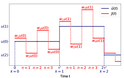
Figure 1: Schematic representation of the preprocessing step: the discrete input sequence $u(0),\,u(1),\,\dots$ defines the function $\bar{u}(t)$ (blue), which is multiplied by a $\tau^{\prime}$-periodic mask function $\mathcal{M}(t)$ to obtain the preprocessed input $J(t)$ (red). Here the length of the mask vector is $N=4$. The resulting function $J(t)$ enters the reservoir equation (9).

2.2 Step (II): reservoir

Inspired by the previous works [12], we study the reservoir given by the delay-diffential equation

$$\frac{dx}{dt}(t)=-x(t)+f[x(t-\tau)+\gamma J(t)],$$ (9)

where $\tau>0$ is the delay-time, $\gamma>0$ is the input strength, $f\colon\mathbb{R}\to\mathbb{R}$ the activation function, and $J(t)$ the preprocessed input function. For a given preprocessed input $J(t)$, the reservoir variable $x(t)$ is computed by solving the delay differential equation (9) with an initial history function $x_{0}(s),$ $s\in[-\tau,0]$. In order for the reservoir to be consistent, the reservoir state $x(t)$ for sufficiently large $t>0$ should depend only on the input $J$ and be independent on the initial state $x_{0}(s)$. In other words, identical reservoirs which are driven by the same input but have different initial states will approximate each other asymptotically. In the literature about reservoir computing this property is often referred to as echo state property or fading memory property [1]. In the literature about dynamical systems, the phenomenon is called generalized synchronization [20, 21] or asymptotic stability [22, 23].

2.3 Step (III): readout

The continuous reservoir variable $x(t)$ needs to be discretized for the output. For this, the dynamical system is read out every $\theta$ time units. Because every small time window $[k\tau^{\prime}+(n-1)\theta,k\tau^{\prime}+n\theta)$ is fed with its own input $J_{k,n}$, these time windows are often seen as ‘virtual nodes’, and the whole delay system as a ‘virtual network’ [12, 24]. We discretize the reservoir variable correspondingly:

$$X(k):=\begin{pmatrix}X_{1}(k)\\ \vdots\\ X_{N}(k)\end{pmatrix}:=\begin{pmatrix}x((k-1)\tau^{\prime}+\theta)\\ x((k-1)\tau^{\prime}+2\theta)\\ \vdots\\ x((k-1)\tau^{\prime}+N\theta)\end{pmatrix}.$$ (10)

In fact, $X(k)$ is the vector containing the $N$-point discretization of the variable $x(t)$ on the interval $((k-1)\tau^{\prime},k\tau^{\prime}]$. The output $\hat{y}=(\hat{y}(k))_{k\in\mathbb{N}_{0}}$ of the machine learning system is defined as

$$\hat{y}(k)=W^{\mathrm{out}}X(k)+c,$$ (11)

where $W^{\mathrm{out}}$ is an $N$-dimensional row vector and $c\in\mathbb{R}$ is a scalar bias. The output weight variables $W^{\mathrm{out}}$ and $c$ are to be adjusted in the training process and are chosen by linear regression for reservoir computers [1].

3 Effect of the mismatch between delay and clock cycle times

When TDRC was first introduced, the clock cycle $\tau^{\prime}$ for the preprocessing of the input mask was chosen to be equal to the delay $\tau$ [12, 17]. In this case one can easily find an ‘equivalent network’ which is a discrete approximation of the reservoir system. See the suplementery material of [12] or reference [25] for an example. However, recent numerical observations show, that the performance may be improved if one sets $\tau^{\prime}\neq\tau$. The earliest example of this can be arguably found in reference [26].

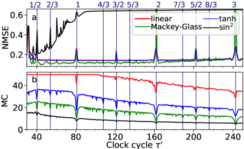
Figure 2: Normalized mean square error (NMSE) of four different TDRCs given in Eq. (9) with nonlinearities of Eqs. (12)-(15) for the NARMA-10 task (top) and the total memory capacity $\mathrm{MC}_{\mathrm{tot}}$ (bottom). Clearly visible are error peaks for values of $\tau^{\prime}$ that are close to integer multiples of $\tau$ and low-order resonances. The presence of the peaks does not depend on the type of the activation function. Vertical lines denote the resonant values of $\tau$ to $\tau^{\prime}$ as indicated on the top axis. The parameters for the simulations are listed in table 1.

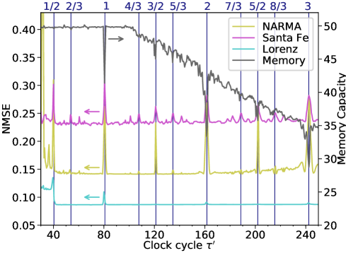
Figure 3: Normalized mean square error (NMSE) for the NARMA-10 task, the Santa Fe time-series task and the Lorenz task (left axis) and the total memory capacity $\mathrm{MC}_{\mathrm{tot}}$ (right axis) of the TDRC of Eq. (9) with linear activation function Eq. (12). For all tasks error peaks (resp. memory capacity drops) are visible for values of $\tau^{\prime}$ that are close to integer multiples of $\tau$ and low-order resonances. Vertical lines denote the resonant values of $\tau$ to $\tau^{\prime}$ as indicated on the top axis. The parameters for the simulations are listed in table 1.

We use the NARMA-10 task [27], the memory capacity (MC) [10], the time series prediction task for the chaotic Lorenz system and the Santa Fe time-series prediction task [28] to measure the performance of a simple TDRC to illustrate the role of the clock cycle $\tau^{\prime}$. These are typical benchmark tasks and we refer to Appendix C-E for a detailed explanation.

Moreover, we use four different functions for the activation function $f$ in equation (9),

linear: $$f(x) =\alpha x,$$ (12)

Mackey-Glass: $$f(x) =\alpha\frac{x}{1+x^{p}},$$ (13)

hyperbolic tangent: $$f(x) =\alpha\tanh(x),$$ (14)

quadratic sin: $$f(x) =\alpha\sin^{2}(x+\varphi),$$ (15)

where we use the parameter values $p=1$ and $\varphi=0.5$. The activation factor is chosen $\alpha=0.9$ for all cases. In fact, the precise choice of the parameter $\alpha$ does not influence qualitatively the phenomenon which we consider, see Appendix F for more details. The other parameters are set to $\tau=80$, $N=50$, and $\gamma=0.02$. For our tests we choose $100$ different input weight vectors $W^{\mathrm{mask}}$ with independently $\mathcal{U}(-1,1)$-distributed entries $w_{n}$. For each input weight vector we train the system with $50000$ training time steps and a Tikhonov regularization with parameter $\beta=10^{-8}$. The training starts after an initial period of $200000$ inputs which is necessary to ensure that the reservoirs initial state does not influence the results. Only then do we record the system state for the next $20000$ inputs, with which we facilitate the training. The only exception are the simulations for the Santa Fe time-series prediction task. Since the Santa Fe dataset contains only about $9000$ data points, we choose aperiod of $4000$ initial inputs, $4000$ training steps and $1000$ test steps. All parameters for the simulations are summarized in table 1. The memory capacity is evaluated up to length $300$. Values that are close to $0$ are not included in the sum. We estimate this overfitting threshold dynamically during the run, by using uncorrelated random target variables.

system parameters
delay-time $\tau$	$80$
input scaling $\gamma$	$0.02$
number of nodes $N$	$50$
activation factor $\alpha$	$0.9$
range of clock cycle $\tau^{\prime}$	$[30,235]$
Mackey-Glass exponent $p$	$1$
phase shift $\varphi$ in activation function (15)	$0.5$
simulation parameters
regularization parameter $\beta$	$10^{-8}$
number of runs (with random mask)	$100$
number of initial steps per run:
$\circ$ for Santa Fe task	$4000$
$\circ$ for all other task	$200000$
number of training steps per run:
$\circ$ for Santa Fe task	$4000$
$\circ$ for all other task	$50000$
number of test steps per run:
$\circ$ for Santa Fe task	$1000$
$\circ$ for all other task	$20000$
time step of $4$th order Runge-Kutta	0.01

Table 1: Parameters for the numerical computation of the NMSE for the NARMA-10, Lorenz and Santa Fe task and the memory capacity of the system.

The top panel of figure 2 shows the results of simulations for the NARMA-10 task for the four different activation functions (12)-(15). The figure shows clear peaks of the error for certain values of the clock cycle $\tau^{\prime}$. These peaks are located close to low-order resonances with the delay-time $\tau=80$ and fulfill the relation $a\tau\approx b\tau^{\prime}$ for small $a,b\in\mathbb{N}$. In fact, the peaks are located slightly above the resonant $\tau^{\prime}$ values. Note, that $tanh$ and the linear function have very similar values. The lower panel of figure 2 depicts the memory capacity and reveals at least part of the reason for this: The total memory capacity for these resonant clock cycles decreases dramatically.

To explore if the observed effect is related to the choice of task, we plot the performance for four different tasks in Figure 3. In each case the linear activation (12) was used. One can see that the error peaks (resp. performance drops) are visible in all tested tasks.

The rest of this paper is devoted to the explanation of this phenomenon. Thereby we focus on the linear activation (12). Lacking a nonlinearity, this is not the optimal choice for the TDRC, the resonance effects that we are interested in seem to be general and independent of $f$ as shown in figure 2, where the performance for the activation functions (12)-(15) is computed. Furthermore, this simplification will allow us to deduce analytical results. In particular, we will be able to show the reason for the drop of the linear memory capacity explicitly.

4 Approximation by a network

In order to explain the degradation of the memory capacity for the resonant clock cycles, we present the time delay-system reservoir as an equivalent network. Similar procedure was done in [12] for a TDRC with $\tau^{\prime}=\tau$ and arbitrary activation function. Here we present a derivation of an equivalent network for the case $\tau^{\prime}\neq\tau$, where the results of [12] cannot be applied. However, we have to restrict it to a linear activation function in order to obtain an explicit network representation.

An alternative way to describe the dependence of $X(k+1)$ on $X(k)$ and the input for the case $\tau^{\prime}\neq\tau$ is presented in [29], where the authors use an integral formula instead of a network formulation. This integral formula includes the case of a nonlinear activation function. For our explanation of the observed memory capacity drops, the network representation presented in this section is, however, indispensable.

Since a detailed derivation is technical, we move it to Appendix A and present the main results in this section.

As follows from Appendix A, the TDRC dynamics can be approximated by the discrete mapping

$$\begin{split}\tilde{X}(k+1)=B\tilde{X}(k)+(1-e^{-\theta})F\left[A_{q}\tilde{X}(k+1-\ell)\right.\\ \left.+A_{-(N-q)}\tilde{X}(k-\ell)+\gamma J_{k}\right],\end{split}$$ (16)

where

$$\tilde{X}(k):=A_{0}^{-1}X(k)$$ (17)

and $X(k)$ is the discretized vector of the reservoir defined in equation (10). Let us define and explain further notations used in the mapping (16). The matrix

$$A_{0}:=\begin{pmatrix}1&0&\dots&0\\ e^{-\theta}&1&\ddots&\vdots\\ \vdots&\ddots&\ddots&0\\ e^{-(N-1)\theta}&\dots&e^{-\theta}&1\end{pmatrix}$$ (18)

is the classical coupling matrix of an equivalent network for TDRC with $\tau^{\prime}=\tau$ [12]. Moreover,

$$\begin{split}\ell&:=\left\lfloor\frac{m}{N}\right\rfloor,\quad q:=m\text{ mod }N,\\ m&:=\left\lceil\frac{\tau}{\theta}\right\rceil=\left\lceil\frac{\tau}{\tau^{\prime}}N\right\rceil,\quad\theta=\frac{\tau^{\prime}}{N},\end{split}$$ (19)

where $\lfloor\cdot\rfloor$ and $\lceil\cdot\rceil$ denote the floor and the ceiling function, which we need to employ to allow delay-times $\tau$ that are not an integer multiple of the time per virtual node $\theta$. These quantities can be interpreted as follows: $m$ is the number of virtual nodes that are needed to cover a $\tau$-interval, $q$ is a measure of the misalignment between $\tau$ and $\tau^{\prime}$, and $\ell$ is roughly the ratio between the delay-time $\tau$ and the clock cycle $\tau^{\prime}$. For $\ell=0$, the delay $\tau$ is shorter than the clock cycle $\tau^{\prime}$, and it is similar to or larger than the clock cycle for $\ell\geq 1$. The matrices $A_{q}$ and $A_{-(N-q)}$ are shifted versions of the matrix $A_{0}$. They are defined as follows:

$$A_{q}:=\begin{pmatrix}0&\cdots&\cdots&\cdots&\cdots&\cdots&0\\ \vdots&&&&&&\vdots\\ 0&&&&&&\vdots\\ 1&0&&&&&\vdots\\ e^{-\theta}&1&\ddots&&&&\vdots\\ \vdots&\ddots&\ddots&0&&&\vdots\\ e^{-(N-1-q)\theta}&\cdots&e^{-\theta}&1&0&\cdots&0\end{pmatrix}$$ (20)

is obtained by a downwards shift of $A_{0}$ by $q$ rows and

$$A_{-(N-q)}:=\\ \begin{pmatrix}e^{-(N-q)\theta}&\cdots&e^{-2\theta}&e^{-\theta}&1&0&\cdots&0\\ \vdots&&&\ddots&\ddots&\ddots&\ddots&\vdots\\ \vdots&&&&\ddots&\ddots&\ddots&0\\ e^{-(N-1)\theta}&\cdots&\cdots&\cdots&\cdots&e^{-2\theta}&e^{-\theta}&1\\ 0&\cdots&\cdots&\cdots&\cdots&0&0&0\\ \vdots&&&&&&&\vdots\\ 0&\cdots&\cdots&\cdots&\cdots&\cdots&\cdots&0\end{pmatrix}$$ (21)

is obtained by the upwards shift of $A_{0}$ by $N-q$ rows. Furthermore

$$B:=\begin{pmatrix}e^{-N\theta}&\dots&e^{-\theta}\\ 0&\dots&0\\ \vdots&&\vdots\\ 0&\dots&0\end{pmatrix},$$ (22)

$$F\begin{pmatrix}x_{1}\\ \vdots\\ x_{N}\end{pmatrix}:=\begin{pmatrix}f(x_{1})\\ \vdots\\ f(x_{N})\end{pmatrix},$$ (23)

and $J_{k}$ is defined as the input vector (8).

The mapping (16) generalizes previous results from [12, 24]. If the clock cycle $\tau^{\prime}$ satisfies $\tau^{\prime}\in[\tau,\tau+\theta)$, the description coincides with the classical case $\tau^{\prime}=\tau$ and the approximate equation (16) yields the same mapping

$$\tilde{X}(k+1)=B\tilde{X}(k)+(1-e^{-\theta})F[A_{0}\tilde{X}(k)+\gamma J_{k}]$$ (24)

as presented in [12] because then $\ell=1$, $q=0$, and $A_{-(N-q)}=0$.

Analytical approaches for the nonlinear system (16) are challenging. To simplify, we will study the effect of different clock cycles $\tau^{\prime}$ with the help of a linear activation function $f(x)=\alpha x$, where $\alpha$ is a scalar. Then equation (16) can be written as

$$\begin{split}\tilde{X}(k+1)&=B\tilde{X}(k)+\nu\alpha[A_{q}\tilde{X}(k+1-\ell)\\ &\hphantom{{}=}+A_{-(N-q)}\tilde{X}(k-\ell)+\gamma W^{\mathrm{mask}}u(k)]\end{split}$$ (25)

by plugging in $W^{\mathrm{mask}}u(k)$ for $J_{k}$ and by writing $\nu:=1-e^{-\theta}$ for the sake of shortness.

System (16) possesses the following properties: in the case $\tau^{\prime}\geq\tau+\theta$, we have $\ell=0$, and hence, equation (16) is in general an implicit map. This is the physical case of a delay shorter than the clock cycle, which means that the feedback from some of the virtual nodes will act on other virtual nodes within the same cycle. However, for the linear activation function in equation (25) and by (17) we obtain for the case $\ell=0$ the explicit map

$$X(k+1)=AX(k)+W^{\mathrm{in}}u(k),$$ (26)

where

$$A:=A_{0}(\mathrm{Id}-\nu\alpha A_{q})^{-1}(B+\nu\alpha A_{-(N-q)})A_{0}^{-1}$$ (27)

is a matrix that describes the coupling and local dynamics of the virtual network and

$$W^{\mathrm{in}}:=\nu\alpha\gamma A_{0}(\mathrm{Id}-\nu\alpha A_{q})^{-1}W^{\mathrm{mask}}$$ (28)

is the generalized input matrix.

Equation (26) is the main result of this section. It shows that the TDRC system can be modeled by an equivalent network for $\tau^{\prime}\geq\tau+\theta$ if its activation function $f$ is linear. In previous publications [12] such a network representation was derived for the case $\tau^{\prime}=\tau$, however, in that case also for nonlinear activation functions.

An important observation from Eq. (26) is that the spectral radius of the matrix $A$ must be smaller than one, otherwise the system (26) will not be asymptotically stable. We achieve this by choosing appropriate parameter $\alpha=0.9$ (see figure 7 in Appendix F).

Equation (26) allows us to calculate directly some figures of merit in the following. We first use it to explain the drops in the memory capacity in figure 2 for resonant delays. One important aspect to note, is that the basic shape of equation (26) does not change with $\tau^{\prime}$. Rather, a changing of the clock cycle leads to a change of the evolution matrices $A$ and $W^{\mathrm{in}}$ of the equivalent network. The obtained system (26) can be equivalently considered as a specific echo state network.

5 Direct calculation of memory capacity

One can find an estimation for the memory capacity of a reservoir computing system by solving the system numerically and let it perform the memory task. But there are also analytic methods for some cases. In this section we explain how to calculate analytically the memory capacity of the linear echo state network (26) which corresponds to the case $\tau^{\prime}\geq\tau+\theta$.

Memory capacity was originally defined by Jaeger in [10]. In the following, we use a slightly modified formulation. Let the elements $u(k)$ of the input sequence be independently $\mathcal{N}(0,1)$-distributed. Jaeger introduced the quantity $\mathrm{MC}_{d}$ which indicates how well the output $\hat{y}(k)$ of an ESN may approximate the input value $u(k-d)$ which was fed into the reservoir $d$ time steps earlier. The memory capacity for a recall of $d$ time steps in the past is defined by

$$\mathrm{MC}_{d}:=\max_{W^{\mathrm{out}}}\left(1-\frac{\mathrm{E}[(W^{\mathrm{out}}X(k+d)-u(k))^{2}]}{\mathrm{var}(u(k))}\right),$$ (29)

where $\mathrm{E}$ denotes the expectation value and we require the initial state $X(0)$ of the reservoir to be stationary distributed in order to ensure that this definition is consistent, i.e. that the distribution of $X(k)$ does not depend on $k$. Since the spectral radius of $A$ is less than one, the stationary distribution exists. In such a case, the memory capacity (29) with stationary distributed $X(0)$ can be equivalently written as

$$\begin{split}\mathrm{MC}_{d}&:=\max_{W^{\mathrm{out}}}\left(1-\frac{\mathrm{E}[(W^{\mathrm{out}}X(d)-u(0))^{2}]}{\mathrm{var}(u(0))}\right)\\ &\hphantom{:}=1-\min_{W^{\mathrm{out}}}\mathrm{E}[(W^{\mathrm{out}}X(d)-u(0))^{2}].\end{split}$$ (30)

Note that $u(0)\sim\mathcal{N}(0,1)$ means that we can drop the term $\mathrm{var}(u(0))$ in (30).

The total memory capacity $\mathrm{MC}$ is defined as the sum of all $d$-step memory capacities

$$\mathrm{MC}:=\sum_{d=1}^{\infty}\mathrm{MC}_{d}.$$ (31)

In the following we denote the optimal output weight vector for (30) by $W_{d}^{\mathrm{out}}$. Let $\Sigma$ be the covariance matrix of the stationary distribution of the reservoir. Jaeger [10] noted that, if $\Sigma$ is invertible, one can apply the Wiener-Hopf equation [30] to find

$$W_{d}^{\mathrm{out}}=(A^{d-1}W^{\mathrm{in}})^{\mathrm{T}}\Sigma^{-1}.$$ (32)

For details we refer to Appendix B. Using this optimal value $W_{d}^{\text{out}}$, the memory capacity (30) can be calculated as

$$\mathrm{MC}_{d}=(A^{d-1}W^{\mathrm{in}})^{\mathrm{T}}\Sigma^{-1}A^{d-1}W^{\mathrm{in}},$$ (33)

where we have used the relations

$$\begin{split}\mathrm{E}[W_{d}^{\mathrm{out}}X(d)u(0)]&=\mathrm{cov}(W_{d}^{\mathrm{out}}X(d),u(0))\\ &=(A^{d-1}W^{\mathrm{in}})^{\mathrm{T}}\Sigma^{-1}A^{d-1}W^{\mathrm{in}}\end{split}$$ (34)

and

$$\begin{split}\mathrm{E}[(W_{d}^{\mathrm{out}}X(d))^{2}]&=\mathrm{var}(W_{d}^{\mathrm{out}}X(d))\\ &=(A^{d-1}W^{\mathrm{in}})^{\mathrm{T}}\Sigma^{-1}A^{d-1}W^{\mathrm{in}}.\end{split}$$ (35)

So once the covariance matrix of the reservoir $X$ is invertible, one can directly calculate the memory capacity. The stationary distribution of system (26) with standard normal distributed input elements $u(k)$ is a multivariate normal distribution with mean zero and covariance matrix

$$\Sigma=\sum_{j=0}^{\infty}A^{j}W^{\mathrm{in}}(W^{\mathrm{in}})^{\mathrm{T}}A^{j\mathrm{T}}.$$ (36)

We refer to Appendix B for a derivation. It is worth to comment on the structure of the matrix $\Sigma$. We note that the summands $A^{j}W^{\mathrm{in}}(W^{\mathrm{in}})^{\mathrm{T}}A^{j\mathrm{T}}$ in (36) are rank one symmetric matrices with the norm $\|A^{j}W^{\mathrm{in}}\|^{2}$. Since the spectral radius of $A$ is less than one, this norm converges to zero as $j\to\infty$ and there is only a finite number of terms in (36) which can make numerically significant contribution to the rank of $\Sigma$. In addition, as we will see in the following, these rank-one matrices may have almost coinciding eigenspaces. As a result, the matrix $\Sigma$ is in general numerically not invertible. Since our approach for the derivation of equation (33) relies on the invertibility of $\Sigma$, we cannot simply replace $\Sigma^{-1}$ by a pseudo-inverse. In order to obtain an invertible covariance matrix, we need to perturb the stochastic process (26). We choose a small number $\sigma_{\eta}>0$ and let $\eta(k)\sim\mathcal{N}(0,\mathrm{Id})$ be a sequence of independent multivariate normal distributed random variables. The stochastic process

$$X(k+1)=AX(k)+W^{\mathrm{in}}u(k)+\sigma_{\eta}\eta(k),$$ (37)

has the stationary distribution $\mathcal{N}(0,\Sigma_{\eta})$ where the covariance matrix given by

$$\Sigma_{\eta}=\sum_{j=0}^{\infty}A^{j}(W^{\mathrm{in}}(W^{\mathrm{in}})^{\mathrm{T}}+\sigma_{\eta}\mathrm{Id})A^{j\mathrm{T}}$$ (38)

is invertible.

6 Explanation for memory capacity gaps

Using the expressions (31) and (33) for the memory capacity obtained in section 5, we provide an explanation for the loss of the memory capacity when $\tau^{\prime}/\tau$ is close to rational numbers with small denominator. The explanation is based on the structure of the covariance matrix $\Sigma_{\eta}$ given by equation (38) and the corresponding expression for the memory capacity, which we repeat here for convenience

$$\begin{split}\mathrm{MC}&=\sum_{d=1}^{\infty}\mathrm{MC}_{d},\\ \mathrm{MC}_{d}&=(A^{d-1}W^{\mathrm{in}})^{\mathrm{T}}\Sigma_{\eta}^{-1}A^{d-1}W^{\mathrm{in}},\end{split}$$ (39)

where

$$\begin{split}\Sigma_{\eta}&:=\sum_{j=0}^{\infty}(\Pi_{j}+\sigma_{\eta}A^{j}A^{j\mathrm{T}}),\\ \Pi_{j}&:=A^{j}W^{\mathrm{in}}(W^{\mathrm{in}})^{\mathrm{T}}A^{j\mathrm{T}}.\end{split}$$ (40)

Our further strategy is as follows:

• Firstly, we remark that the norms of the individual terms in the sum (40) are converging to zero due to the convergence of the series. Hence, only the first finitely many terms play an important role. For instance, for our previously chosen parameters in figure 2, the terms with $j\gtrsim 30$ do not make a large contribution and can be neglected. In the following we denote the approximate number of significant terms by $j_{n}$.

• We show that the largest eigenvalue of the $j$-th term in (40) can be approximated by $\|A^{j}W^{\text{in}}\|^{2}$ with the corresponding eigenvector $A^{j}W^{\text{in}}$.

• We show that the memory capacity is high, i.e. $\mathrm{MC}_{d}\approx 1$ for $d\leq j_{n}$, when the eigenvectors $A^{j}W^{\text{in}}$ corresponding to the first relevant terms in the sum (40) are orthogonal.

• Using our setup, we show numerically that the lower order resonances $\tau^{\prime}/\tau\approx a/b$, where $a,b\in\mathbb{N}$ and $b$ is small, lead to the alignment of the eigenvectors $A^{j}W^{\text{in}}$, and hence, to the loss of the memory capacity. The small shift from the exact resonance values is explained by the standard drift property of delay systems.

• Finally we give an intuitive explanation of the obtained orthogonality conditions.

(i) Convergence of the series (40)

The series (40) can be considered as the Neumann series $(\mathrm{Id}-T)^{-1}=\sum_{j=0}^{\infty}T^{j},$ where $T\mathcal{X}:=A\mathcal{X}A^{\mathrm{T}}$, applied to the matrix $W^{\mathrm{in}}(W^{\mathrm{in}})^{\mathrm{T}}+\sigma_{\eta}\mathrm{Id}$. A sufficient condition for the convergence of such a series is that $\|T^{k}\|_{\mathrm{op}}:=\sup_{\|\mathcal{X}\|=1}\|T^{k}\mathcal{X}\|<1$ for some $k>0$, where $\|\cdot\|$ is some matrix norm. Moreover, $\|T^{k}\mathcal{X}\|=\|A^{k}\mathcal{X}A^{k\mathrm{T}}\|\leq\|A^{k}\|\|\mathcal{X}\|\|A^{k\mathrm{T}}\|=\|A^{k}\|^{2}$ when $\|\mathcal{X}\|=1$. Since the spectral radius of $A$ is smaller than one, Gelfand’s formula implies that there is a number $k>0$ such that $\|A^{k}\|<1$, and hence, the sufficient condition $\|T^{k}\|_{\mathrm{op}}<1$ for the convergence of the series is satisfied.

(ii) Estimating the largest eigenvalues and eigenvectors of the $j$-th term in (40)

Consider at first the term with $j=0$: $W^{\mathrm{in}}(W^{\mathrm{in}})^{\mathrm{T}}+\sigma_{\eta}\mathrm{Id}.$ The largest eigenvalue of this matrix is $\|W^{\mathrm{in}}\|_{2}^{2}+\sigma_{\eta}$ and the corresponding eigenvector is $W^{\mathrm{in}}$ as can be easily checked by the direct calculation

$$[W^{\mathrm{in}}(W^{\mathrm{in}})^{\mathrm{T}}+\sigma_{\eta}\mathrm{Id}]W^{\mathrm{in}}=(\|W^{\mathrm{in}}\|_{2}^{2}+\sigma_{\eta})W^{\mathrm{in}}.$$ (41)

For all other eigenvectors $v$, which are orthogonal to $W^{\mathrm{in}}$ due to the symmetry of the matrix, the corresponding eigenvalues are $\sigma_{\eta}$ because

$$[W^{\mathrm{in}}(W^{\mathrm{in}})^{\mathrm{T}}+\sigma_{\eta}\mathrm{Id}]v=W^{\mathrm{in}}\langle W^{\mathrm{in}},v\rangle+\sigma_{\eta}v=\sigma_{\eta}v.$$ (42)

These eigenvalues are by definition small, since $\sigma_{\eta}$ is a small perturbation.

We can also find approximations of the eigenvectors and eigenvalues for the higher order terms $\Pi_{j}+\sigma_{\eta}A^{j}A^{j\mathrm{T}}$, $j>0$. Namely, for the unperturbed matrix $\Pi_{j}$, the largest eigenvalue is $\|A^{j}W^{\mathrm{in}}\|^{2}$ and the corresponding eigenvector is $A^{j}W^{\mathrm{in}}$ because

$$\begin{split}\Pi_{j}A^{j}W^{\mathrm{in}}&=[A^{j}W^{\mathrm{in}}(W^{\mathrm{in}})^{\mathrm{T}}A^{j\mathrm{T}}]A^{j}W^{\mathrm{in}}\\ &=A^{j}W^{\mathrm{in}}\langle A^{j}W^{\mathrm{in}},A^{j}W^{\mathrm{in}}\rangle\\ &=\|A^{j}W^{\mathrm{in}}\|_{2}^{2}A^{j}W^{\mathrm{in}}.\end{split}$$ (43)

All other eigenvalues are zero. Since the largest eigenvalue of $\Pi_{j}$ is geometrically and algebraically simple, it is continuous under the perturbation by $\sigma_{\eta}\mathrm{Id}$. Hence, the largest eigenvalue and the eigenvector of $\Pi_{j}+\sigma_{\eta}A^{j}A^{j\mathrm{T}}$ are approximated by $\|A^{j}W^{\mathrm{in}}\|^{2}$ and $A^{j}W^{\mathrm{in}}$ with an error of order $\sigma_{\eta}$. All other eigenvalues are correspondingly small of order $\sigma_{\eta}$.

(iii) The orthogonality of $A^{j}W^{\mathrm{in}}$ leads to the high memory capacity

Let $j_{n}$ be the number of terms in (40) that are significant (see (i)), and let us assume that the eigenvectors $A^{j}W^{\mathrm{in}}$, $j=0,1,\dots,j_{n}$ are close to be orthogonal, i.e.

$$\left|\left\langle A^{j}W^{\mathrm{in}},A^{i}W^{\mathrm{in}}\right\rangle\right|\ll 1,\quad i,j=0,1,\dots,j_{n},\,\,\,j\neq i.$$ (44)

As we will see in (iv), such an assumption is indeed reasonable in our setup. More precisely, one could consider (44) as $\left|\left\langle A^{j}W^{\mathrm{in}},A^{i}W^{\mathrm{in}}\right\rangle\right|<\varepsilon$ introducing another small parameter $\varepsilon\ll 1$.

In case, when the orthogonality (44) holds, the largest eigenvalues of $\Sigma_{\eta}$ and their corresponding eigenvectors can be approximated by $\|A^{j}W^{\mathrm{in}}\|^{2}$ and $A^{j}W^{\mathrm{in}}$, $j=0,\dots,j_{n}$. Indeed

$$\begin{split}\Sigma_{\eta}A^{j}W^{\mathrm{in}}&=\sum_{k=0}^{\infty}(\Pi_{k}A^{j}W^{\mathrm{in}}+\sigma_{\eta}A^{k}A^{k\mathrm{T}}A^{j}W^{\mathrm{in}})\\ &=\|A^{j}W^{\mathrm{in}}\|_{2}^{2}A^{j}W^{\mathrm{in}}+\mathcal{O}(\sigma_{\eta})+\mathcal{O}(\varepsilon).\end{split}$$ (45)

In this case, the memory capacity can be calculated as follows:

$$\begin{split}&\text{MC}_{d}=(A^{d-1}W^{\mathrm{in}})^{\mathrm{T}}\Sigma_{\eta}^{-1}A^{d-1}W^{\mathrm{in}}\\ &=(A^{d-1}W^{\mathrm{in}})^{\mathrm{T}}\frac{1}{\|A^{d-1}W^{\mathrm{in}}\|_{2}^{2}}A^{d-1}W^{\mathrm{in}}+\mathcal{O}(\sigma_{\eta})+\mathcal{O}(\varepsilon)\\ &=1+\mathcal{O}(\sigma_{\eta})+\mathcal{O}(\varepsilon)\end{split}$$ (46)

for $d\leq j_{n}$. Hence, the orthogonality of the vectors $A^{j}W^{\mathrm{in}}$ with $A^{i}W^{\mathrm{in}}$, $i\neq j$ guarantees a high memory capacity. We will present an intuitive explanation for this shortly.

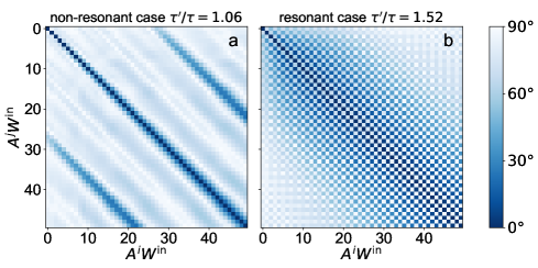
Figure 4: The angles between $A^{j}W^{\mathrm{in}}$ and $A^{i}W^{\mathrm{in}}$, $i,j=1,\dots,50$ are plotted in color, measuring, in particular, the orthogonality of the vectors $A^{j}W^{\mathrm{in}}$ with different $j$. Panels (a) and (b) correspond to different ratios of $\tau^{\prime}/\tau$: (a) $\tau^{\prime}/\tau=1.06$; (b) $\tau^{\prime}/\tau=1.52\gtrsim 3/2$. The former is off-resonant, while the later is close to the $3/2$ resonance, in particular when the drift property of the DDE system is taken into account. In (b) the vectors $A^{j}W^{\mathrm{in}}$ point into the same direction for $j$, $j+2$, $j+4$, etc., i.e. after two time steps the input values $u(k)$ overlap in the state space of $X$ and the memory capacity drops. In contrast, in the case $\tau^{\prime}/\tau=1.06$ (a) it takes almost 30 time steps before the input overlaps with past inputs in the network state. This explains the high memory capacity in this case, which is illustrated in figure 2.

(iv) Resonances of $\tau^{\prime}$ and $\tau$ lead to lower memory capacity

The plots in figure 4 show $\left\langle A^{j}W^{\mathrm{in}},A^{i}W^{\mathrm{in}}\right\rangle$ for different ratios $\tau^{\prime}/\tau$. White to light blue off-diagonal squares indicate that assumption (44) is satisfied, i.e. orthogonal or almost orthogonal vectors. Dark blue indicates a strong parallelism of the vectors. As can bee seen in the top panel of figure 4, the assumption (44) holds indeed for ratios $\tau^{\prime}/\tau$ which yield a good memory performance. Conversely, it is strongly violated for critical ratios $\tau^{\prime}/\tau\gtrsim a/b$ with small denominator $b$, e.g. the center panel of figure 4.

We note that the critical ratios $\tau^{\prime}/\tau$ are slightly shifted from the exact resonant values $1$, $3/2$, etc. This shift is a manifestation of the ‘drift’ property of delay systems [16], which is caused by the fact that the effective round-trip of a signal in a delay system equals to the delay $\tau$ plus a finite processing time $\delta$ due to the integration (filtering). Therefore, the small shift of the error peaks is actually due to a resonance between the clock cycle $\tau^{\prime}$ and $\tau+\delta$. This fact can be seen also in the structure of the coupling matrix $A$ of the equivalent network.

(v) Intuitive explanations

There is an additional intuitive understanding of the above derived formulas. Recall that the original system of the reservoir of equation (9) combines the delay term $x(t-\tau)$ and the input $J(t)$ additively. The approximated network formula for an equivalent network translated this into the matrix $A$, which describes the free dynamics of the network, and the driving term defined by $W^{\mathrm{in}}$. The state of the network is given by an $N$-dimensional system, and thus can at most hold $N$ orthogonal dimensions [31]. Each summand of $\Sigma_{\eta}$ can now be understood as an imprint of the driving term on the system after $j$ time steps. For $j=0$ the matrix $A^{0}=\mathrm{Id}$, and thus the imprint is given by $W^{\mathrm{in}}$, i.e. the information of the current step is stored in the nodes as given by the weights of the effective input weight vector $W^{\mathrm{in}}$. In the next step, the system will get an additional input, but also evolve according to its local dynamics $A$. Thus, after one time step, the imprint has transformed into $AW^{\mathrm{in}}$, i.e. the summand for $j=1$ and $\sigma_{\eta}\to 0$. Now in every step, the information that is currently present in the network will be ‘rotated’ in the phase space of the network according to $A$, while a new input will be projected onto the direction of $W^{\mathrm{in}}$. This holds in general, so that the $j$-th summand of $\Sigma_{\eta}$ of equation (38) $A^{j}W^{\mathrm{in}}$ describes the linear imprint of the input $j$ steps in the past.

The orthogonality condition of equation (44) then is the same concept as demanding that new information from the inputs should not overwrite the already present information. If $A^{r}\approx s\mathrm{Id}$ for some $s\in\mathbb{R}$, then the information that was stored from $r$ steps in the past will be partially overwritten by the currently injected step and lost. Hence, ensuring that the orthogonality between $A^{j}W^{\mathrm{in}}$ is fulfilled as much as possible will maximize the linear memory. For the case of resonant feedback, i.e. $\tau^{\prime}=\tau$, this condition is not fulfilled. This is due to the fact, that $A$ has a strong diagonal component for the resonant cases, i.e. virtual nodes are most strongly coupled to themselves. This is a simple consequence of the fact that for $\tau=\tau^{\prime}$, virtual nodes return to the single real node at the same time that they are updated. Similarly, for higher resonant cases $b\tau^{\prime}=a\tau$, $A^{b}$ will in general have a strong diagonal part and thus the eigenvector $A^{b}W^{in}$ will not be orthogonal to $A^{0}W^{in}$, and the information will be overwritten.

7 Discussion

In this paper we have shown a generalization of the frequently used time-delay reservoir computing for cases other than $\tau^{\prime}=\tau$. We observed that a sudden increase in the computing error (NARMA-10, Lorenz, and Santa-Fe NRMSE) and a drop in the linear memory capacity ($\mathrm{MC}$) can be seen for resonant cases of $b\tau^{\prime}\approx a\tau$ with $a,b\in\mathbb{N}$ where $b$ is small for different activation functions including the linear, $\tanh$, $\sin^{2}$, and the Mackey-Glass function. We derived an equivalent network for the case $\tau^{\prime}\geq\tau+\theta$ which extends the previously studied case $\tau^{\prime}=\tau$. Assuming a linear activation function $f(x)=\alpha x$, we can analytically solve the resulting implicit equations and obtain an expression for the total memory capacity $\mathrm{MC}$. Here we find that the resulting memory capacity will be small for cases where $\tau$ and $\tau^{\prime}$ are resonant because the information within the equivalent network will be overwritten by new inputs very quickly. Even though our analytics so far are only derived for the linear case, we expect these results to hold in more general situations, as numerical simulations with several different nonlinear activation functions in figures 2, 7, 8 indicate. More detailed analysis can be performed in future studies.

Appendix

A Derivation of equivalent networks

This section presents a detailed derivation of the ESN represention of TDRC systems. The derivation is structured as follows:

1. The delay system (9) is discretized such that the state of a virtual node $x(k\tau^{\prime}+n\theta)$ depends on the state of its neighbor node $x(k\tau^{\prime}+(n-1)\theta)$, the input $J_{k,n}$ and the state of a second node $x(k^{\prime}\tau^{\prime}+n^{\prime}\theta)$ at the time $k^{\prime}\leq k$. In order to do so, we approximate the integral of the continuous TDRC system on a small integration interval of length $\theta$ which covers the point $x(k^{\prime}\tau^{\prime}+n^{\prime}\theta)$.

2. The formulas for $n^{\prime}$ and $k^{\prime}$ are derived.

3. The TDCR system can be written as a matrix equation. For this we use the same vectorization (10) of $x(t)$ as for the readout. An recurrent argument is employed to obtain the matrix equation.

4. It follows that the discretized TDRC system can be represented by an ESN if $\tau\leq\tau^{\prime}-\theta$ and if the activation function $f$ is linear.

5. For the sake of completeness, we formulate the equivalent ESN for the classical case $\tau^{\prime}=\tau$, which was described in [12].

A.1 The delay reservoir system and discretization

Consider the delay-system (9), which we repeat here for convenience:

$$\dot{x}(t)=-x(t)+f[x(t-\tau)+\gamma J(t)],$$ (47)

where $\tau>0,\ \gamma>0$ and $f\colon\mathbb{R}\to\mathbb{R}$.

It follows that

$$e^{t-t_{0}}x(t)=x(t_{0})+\int_{t_{0}}^{t}e^{s-t_{0}}f[x(s-\tau)+\gamma J(s)]\,\mathrm{d}s$$ (48)

for $t\geq t_{0}$. Set $t_{0}=k\tau^{\prime}+(n-1)\theta$ and $t=k\tau^{\prime}+n\theta$. Then

$$\begin{split}&x(k\tau^{\prime}+n\theta)=e^{-\theta}x(k\tau^{\prime}+(n-1)\theta)\\ &+\int_{0}^{\theta}e^{s-\theta}f[x(k\tau^{\prime}+(n-1)\theta+s-\tau)+\gamma J_{k,n}]\,\mathrm{d}s,\end{split}$$ (49)

where $J_{k,n}$ is defined in (7). One option to discretize the system, is to approximate the function $x$ by a step function with step length $\theta$ which is constant on the integration interval. One can find an appropriate step function by choosing $k^{\prime}(k,n)$ and $n^{\prime}(n)$ such that

$$k^{\prime}\tau^{\prime}+n^{\prime}\theta\in(k\tau^{\prime}+(n-1)\theta-\tau,k\tau^{\prime}+n\theta-\tau]$$ (50)

and defining $x(t)\approx\tilde{x}(t):=x(k^{\prime}\tau^{\prime}+n^{\prime}\theta)$ for $t\in(k\tau^{\prime}+(n-1)\theta-\tau,k\tau^{\prime}+n\theta-\tau]$. Then, one can replace $x$ by $\tilde{x}$ in the integrand in equation (49). This yields

$$\begin{split}&x(k\tau^{\prime}+n\theta)\\ &\approx e^{-\theta}x(k\tau^{\prime}+(n-1)\theta)\\ &\hphantom{{}=}+\int_{0}^{\theta}e^{s-\theta}f[x(k^{\prime}(k,n)\tau^{\prime}+n^{\prime}(n)\theta)+\gamma J_{k,n}]\,\mathrm{d}s\\ &=e^{-\theta}x(k\tau^{\prime}+(n-1)\theta)\\ &\hphantom{{}=}+(1-e^{-\theta})f[x(k^{\prime}(k,n)\tau^{\prime}+n^{\prime}(n)\theta)+\gamma J_{k,n}].\end{split}$$ (51)

A.2 The choice of $k^{\prime}$ and $n^{\prime}$

The floor and the ceiling function are denoted by $\lfloor\cdot\rfloor$ and $\lceil\cdot\rceil$, respectively. One can choose $k^{\prime}$ and $n^{\prime}$ in the following way:

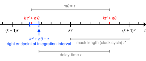
Figure 5: The time interval over which the function $x$ is integrated in equation (49) is highlighted in blue. As stated is equation (50), the point $k^{\prime}\tau^{\prime}+n^{\prime}\theta$ must be chosen such that it lies within this interval. In equation (51) the value of $x$ on the integration interval is approximated by the value of $x(k^{\prime}\tau^{\prime}+n^{\prime}\theta)$. If the endpoints of the interval are grid points, $k^{\prime}\tau^{\prime}+n^{\prime}\theta$ is chosen to be the right endpoint.

First, let $m\in\mathbb{Z},\ m\geq 1$ be the unique number such that $\tau\in((m-1)\theta,m\theta]$, i.e. $m=\lceil\tau/\theta\rceil$. Then

$$k^{\prime}\tau^{\prime}+n^{\prime}\theta=k\tau^{\prime}+n\theta-m\theta$$ (52)

as illustrated in figure 5. Now, the choice of $n^{\prime}$ follows directly from the restriction $n^{\prime}\in\{1,\ldots,N\}$. It holds that

$$n^{\prime}(n)=\begin{cases}(n-m)\mod N,&\text{if }N\nmid(n-m),\\ N,&\text{if }N\mid(n-m).\end{cases}$$ (53)

From this result follows that

$$\begin{split}(n-m)\theta&=n^{\prime}\theta+N\theta\cdot\begin{cases}\left\lfloor\frac{n-m}{N}\right\rfloor,&\text{if }N\nmid(n-m),\\ \frac{n-m}{N}-1,&\text{if }N\mid(n-m),\end{cases}\\ &=n^{\prime}\theta+\left(\left\lceil\frac{n-m}{N}\right\rceil-1\right)\tau^{\prime}.\end{split}$$ (54)

Hence, equation (52) implies

$$k^{\prime}(k,n)=k+\left\lceil\frac{n-m}{N}\right\rceil-1.$$ (55)

Note that one has $k^{\prime}=k$ as long as $n-m\in\{1,n-1\}$. If $n-m\in\{-N+1,\ldots,0\}$, then $k^{\prime}=k-1$. For $n-m\in\{-2N+1,\ldots,-N\}$ holds $k^{\prime}=k-2$, etc.

A.3 Vectorization of the state space and a matrix equation for the discretized system

Define

$$X(k):=\begin{pmatrix}X_{1}(k)\\ \vdots\\ X_{N}(k)\end{pmatrix}:=\begin{pmatrix}x((k-1)\tau^{\prime}+\theta)\\ x((k-1)\tau^{\prime}+2\theta)\\ \vdots\\ x((k-1)\tau^{\prime}+N\theta)\end{pmatrix}$$ (56)

and $\tilde{f}\equiv(1-e^{-\theta})f$. From (51) follows

$$\begin{split}&X_{1}(k+1)=x(k\tau^{\prime}+\theta)\\ &=e^{-\theta}x(k\tau^{\prime})+\tilde{f}[x(k^{\prime}(k,1)\tau^{\prime}+n^{\prime}(1)\theta)+\gamma J_{k,1}]\\ &=e^{-\theta}X_{N}(k)+\tilde{f}[X_{n^{\prime}(1)}(k^{\prime}(k,1)+1)+\gamma J_{k,1}]\end{split}$$ (57)

and repeated application of Eq. (51) yields

$$\begin{split}&X_{n}(k+1)\\ &=e^{-n\theta}X_{N}(k)\\ &\hphantom{{}=}+e^{-(n-1)\theta}\tilde{f}[X_{n^{\prime}(1)}(k^{\prime}(k,1)+1)+\gamma J_{k,1}]\\ &\hphantom{{}=}+e^{-(n-2)\theta}\tilde{f}[X_{n^{\prime}(2)}(k^{\prime}(k,2)+1)+\gamma J_{k,2}]\\ &\hphantom{{}=}\ \ \vdots\\ &\hphantom{{}=}+e^{-\theta}\tilde{f}[X_{n^{\prime}(n-1)}(k^{\prime}(k,n-1)+1)+\gamma J_{k,n-1}]\\ &\hphantom{{}=}+\tilde{f}[X_{n^{\prime}(n)}(k^{\prime}(k,n)+1)+\gamma J_{k,n}]\end{split}$$ (58)

for $n\in\{2,\ldots,N\}$.

These equations can by rewritten as a matrix equation. Let

$$A_{0}:=\begin{pmatrix}1&0&\dots&0\\ e^{-\theta}&1&\ddots&\vdots\\ \vdots&\ddots&\ddots&0\\ e^{-(N-1)\theta}&\dots&e^{-\theta}&1\end{pmatrix}$$ (59)

and

$$\tilde{F}\begin{pmatrix}x_{1}\\ \vdots\\ x_{N}\end{pmatrix}:=\begin{pmatrix}\tilde{f}(x_{1})\\ \vdots\\ \tilde{f}(x_{N})\end{pmatrix}.$$ (60)

Then

$$\begin{split}X(k+1)&=A_{0}\tilde{F}\begin{pmatrix}X_{n^{\prime}(1)}(k^{\prime}(k,1)+1)+\gamma J_{k,1}\\ \vdots\\ X_{n^{\prime}(N)}(k^{\prime}(k,N)+1)+\gamma J_{k,N}\end{pmatrix}\\ &\hphantom{={}}+\begin{pmatrix}e^{-\theta}X_{N}(k)\\ \vdots\\ e^{-N\theta}X_{N}(k)\end{pmatrix}\end{split}$$ (61)

Let $\ell:=\lfloor m/N\rfloor$ and $q:=m\mod N$, as defined in (19), i.e $m=\ell N+q$. By plugging this into equation (53) and noting that $1\leq n\leq N$ and $0\leq q\leq N-1$, one obtains

$$n^{\prime}(n)=\begin{cases}n-q+N,\quad\text{for }n\leq q,\\ n-q,\quad\text{for }n>q,\end{cases}$$ (62)

and by replacing $m$ by $\ell N+q$ equation (55) follows

$$k^{\prime}(k,n)=\begin{cases}k-\ell,&n>q,\\ k-\ell-1,&n\leq q.\end{cases}$$ (63)

Hence, the vector $\left(X_{n^{\prime}(n)}(k^{\prime}(k,n)+1)\right)_{n=1,\ldots,N}$ can be written as follows:

$$\begin{split}\begin{pmatrix}X_{n^{\prime}(1)}(k^{\prime}(k,1)+1)\\ \vdots\\ X_{n^{\prime}(N)}(k^{\prime}(k,N)+1)\end{pmatrix}&=\begin{pmatrix}0\\ \vdots\\ 0\\ X_{1}(k+1-\ell)\\ \vdots\\ X_{N-q}(k+1-\ell)\end{pmatrix}\\ &\hphantom{{}={}}+\begin{pmatrix}X_{N-q+1}(k-\ell)\\ \vdots\\ X_{N}(k-\ell)\\ 0\\ \vdots\\ 0\end{pmatrix}.\end{split}$$ (64)

Thus, the map (61) can be written as

$$\begin{split}&X(k+1):=A_{0}\tilde{F}[M_{q}X(k+1-\ell)\\ &+M_{-(N-q)}X(k-\ell)+\gamma J_{k}]+A_{0}\begin{pmatrix}e^{-\theta}X_{N}(k)\\ 0\\ \vdots\\ 0\end{pmatrix},\end{split}$$ (65)

where the matrices $M_{q}=(\delta_{i,j+q})_{1\leq i,j\leq N}$ and $M_{-(N-q)}=(\delta_{i,j-(N-q)})_{1\leq i,j\leq N}$ are shift matrices.

The matrix $A_{0}$ is invertible and can be used to transform the system. Let $\tilde{X}:=A_{0}^{-1}X$. Then

$$\begin{split}\tilde{X}(k+1)&=B\tilde{X}(k)+\tilde{F}[A_{q}\tilde{X}(k+1-\ell)\\ &\hphantom{{}=}+A_{-(N-q)}\tilde{X}(k-\ell)+\gamma J_{k}],\end{split}$$ (66)

where the matrix

$$A_{q}=M_{q}A_{0}=\\ \begin{pmatrix}0&\cdots&\cdots&\cdots&\cdots&\cdots&0\\ \vdots&&&&&&\vdots\\ 0&&&&&&\vdots\\ 1&0&&&&&\vdots\\ e^{-\theta}&1&\ddots&&&&\vdots\\ \vdots&\ddots&\ddots&0&&&\vdots\\ e^{-(N-1-q)\theta}&\cdots&e^{-\theta}&1&0&\cdots&0\end{pmatrix}$$ (67)

is obtained by a $q$ rows downwards shift of $A_{0}$ and the matrix

$$A_{-(N-q)}=M_{-(N-q)}A_{0}=\\ \begin{pmatrix}e^{-(N-q)\theta}&\cdots&e^{-2\theta}&e^{-\theta}&1&0&\cdots&0\\ \vdots&&&\ddots&\ddots&\ddots&\ddots&\vdots\\ \vdots&&&&\ddots&\ddots&\ddots&0\\ e^{-(N-1)\theta}&\cdots&\cdots&\cdots&\cdots&e^{-2\theta}&e^{-\theta}&1\\ 0&\cdots&\cdots&\cdots&\cdots&0&0&0\\ \vdots&&&&&&&\vdots\\ 0&\cdots&\cdots&\cdots&\cdots&\cdots&\cdots&0\end{pmatrix}$$ (68)

is obtained by an $N-q$ rows upwards shift of $A_{0}$ and

$$B=\begin{pmatrix}e^{-N\theta}&\dots&e^{-\theta}\\ 0&\dots&0\\ \vdots&&\vdots\\ 0&\dots&0\end{pmatrix}.$$ (69)

The equation (69) for matrix $B$ follows from equation (LABEL:eq:matrix_system_shifted). It must hold that

$$\begin{pmatrix}e^{-\theta}X_{N}(k)\\ 0\\ \vdots\\ 0\end{pmatrix}=B\tilde{X}(k)=BA_{0}^{-1}X(k).$$ (70)

Hence,

$$B=\begin{pmatrix}0&\dots&0&e^{-\theta}\\ 0&\dots&\dots&0\\ \vdots&&&\vdots\\ 0&\dots&\dots&0\end{pmatrix}A_{0}.$$ (71)

A.4 An ESN representation of TDRC systems with suitable parameters

If $\tau\leq\tau^{\prime}-\theta$, then $\ell=0$. This follows from the definitions $\ell:=\lfloor m/N\rfloor$ and $m=\lceil\tau/\theta\rceil$. Equation (66) is in this case an implicit map:

$$\begin{split}\tilde{X}(k+1)&=B\tilde{X}(k)\\ &\hphantom{={}}+\tilde{F}[A_{q}\tilde{X}(k+1)+A_{-(N-q)}\tilde{X}(k)+\gamma J_{k}].\end{split}$$ (72)

However, for a linear activation function $f(x)=\alpha x$, where $\alpha$ is a scalar, holds $\tilde{f}(x)=(1-e^{-\theta})\alpha x$ and hence one obtains the explicit linear map

$$\begin{split}\tilde{X}(k+1)&=(\mathrm{Id}-\nu\alpha A_{q})^{-1}(B+\nu\alpha A_{-(N-q)})\tilde{X}(k)\\ &\hphantom{{}=}+\nu\alpha\gamma(\mathrm{Id}-\nu\alpha A_{q})^{-1}J_{k},\end{split}$$ (73)

where $\nu:=1-e^{-\theta}$. Since $\tilde{X}=A_{0}^{-1}X$ and $J_{k}=W^{\mathrm{mask}}u_{k}$, one can write this map in the original coordinates and in terms of the original input sequence

$$X(k+1)=AX(k)+Wu(k),$$ (74)

where

$$A:=A_{0}(\mathrm{Id}-\nu\alpha A_{q})^{-1}(B+\nu\alpha A_{-(N-q)})A_{0}^{-1}$$ (75)

and

$$W^{\mathrm{in}}:=\nu\alpha\gamma A_{0}(\mathrm{Id}-\nu\alpha A_{q})^{-1}W^{\mathrm{mask}}.$$ (76)

The network matrix A is plotted in figure 6 for different parameters.

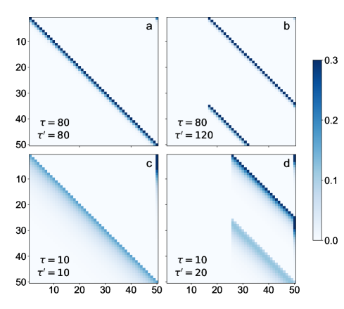
Figure 6: Plot of the network matrix $A$, given by (75) resp. (80), for $N=50$ and diverse values of $\tau$ and $\tau^{\prime}$. The connection weights are truncated at $0.3$. The panels (a) and (c) show matrices for the classical case $\tau=\tau^{\prime}$. (See subsection A.5.) The panels (b) and (d) show matrices for the case $\tau\leq\tau^{\prime}-\theta$ (subsection A.4). These particular examples have resonant values of $\tau$ and $\tau^{\prime}$, in fact we have (b) $\tau^{\prime}/\tau=1.5$ and (d) $\tau^{\prime}/\tau=2$. The strongest connection weights lie on diagonal lines which are shifted as the ratio of $\tau^{\prime}$ and $\tau$ changes. The weights below these lines scale with the factor $e^{-n\theta}$, where $n$ is the distance to the line. Since $\theta=\tau^{\prime}/N$, the (off-diagonal) weights are larger in panels (c) and (d), were $\tau^{\prime}$ is smaller.

A.5 The ESN representation of classical TDRC systems

The article [12] contains a description of an equivalent echo state network for TDRC systems with $\tau^{\prime}=\tau$. This description is consistent with the case $\tau\in(\tau^{\prime}-\theta,\tau^{\prime}]$ in the framework of our discretization. In this case,

$$m=N,\quad\ell=1,\quad q=0,$$ (77)

and therefore, $A_{q}=A_{0}$ and $A_{-(N-q)}$ is the zero matrix. Thus, equation (66) simplifies to

$$\tilde{X}(k+1)=B\tilde{X}(k)+\tilde{F}[A_{0}\tilde{X}(k)+\gamma J_{k}].$$ (78)

For a linear activation function $f(x)=\alpha x$ and $\tau\leq\tau^{\prime}-\theta$, i.e. $\ell=0$, the equivalent network written in the original coordinates is

$$X(k+1)=AX(k)+Wu(k),$$ (79)

where

$$A:=A_{0}BA_{0}^{-1}+\nu\alpha A_{0}$$ (80)

and

$$W^{\mathrm{in}}:=\nu\alpha\gamma A_{0}W^{\mathrm{mask}}.$$ (81)

B Derivation of the memory capacity formula

We consider the linear echo state network

$$X(k+1)=AX(k)+W^{\mathrm{in}}u(k),$$ (82)

where the input elements $u(k)$ are independently $\mathcal{N}(0,1)$-distributed. In section 5 we defined

$$\mathrm{MC}_{d}=\max_{W^{\mathrm{out}}}\left(1-\mathrm{E}[(W^{\mathrm{out}}X(k+d)-u(k))^{2}]\right)$$ (83)

and we claimed that

$$W_{d}^{\mathrm{out}}=(A^{d-1}W^{\mathrm{in}})^{\mathrm{T}}\Sigma^{-1}$$ (84)

is the optimal argument for (83). In the following we show that $W_{d}^{\mathrm{out}}$ is indeed the optimal argument for (83).

In order to maximize (83), we need to minimize the mean square error

$$\begin{split}\mathrm{MSE}&=\mathrm{E}[(W^{\mathrm{out}}X(k+d)-u(k))^{2}]\\ &=\mathrm{E}[(W^{\mathrm{out}}X(k+d))^{2}]+\mathrm{E}[u(k)^{2}]\\ &\hphantom{{}=}-2\mathrm{E}[W^{\mathrm{out}}X(k+d)u(k)].\end{split}$$ (85)

We know that $X(k)\sim\mathcal{N}(0,\Sigma)$ and hence

$$W^{\mathrm{out}}X(k)\sim\mathcal{N}(0,W^{\mathrm{out}}\Sigma(W^{\mathrm{out}})^{\mathrm{T}}).$$ (86)

Note that $W^{\mathrm{out}}\Sigma(W^{\mathrm{out}})^{\mathrm{T}}$ is a scalar because $W^{\mathrm{out}}$ is a row vector. Since the mean of $W^{\mathrm{out}}X(k+d)$ is zero and $u(k)\sim\mathcal{N}(0,1)$, we have

$$\begin{split}\mathrm{E}[(W^{\mathrm{out}}X(k+d))^{2}]&=\mathrm{var}(W^{\mathrm{out}}X(k+d))\\ &=W^{\mathrm{out}}\Sigma(W^{\mathrm{out}})^{\mathrm{T}},\end{split}$$ (87)

$$\mathrm{E}[u(k)^{2}] =1,$$ (88)

$$\mathrm{E}[W^{\mathrm{out}}X(k+d)u(k)] =\mathrm{cov}(u(k),W^{\mathrm{out}}X(k+d)).$$ (89)

Moreover,

$$\begin{split}&W^{\mathrm{out}}X(k+d)\\ &=W^{\mathrm{out}}\left(A^{d}X(k)+\sum_{j=0}^{d-1}A^{j}W^{\mathrm{in}}u(k+d-1-j)\right)\end{split}$$ (90)

and $u(k)$ is independent of $X(k)$. Therefore,

$$\begin{split}&\mathrm{cov}(u(k),W^{\mathrm{out}}X(k+d))\\ &=\mathrm{cov}(u(k),W^{\mathrm{out}}A^{d-1}W^{\mathrm{in}}u(k))\\ &=W^{\mathrm{out}}A^{d-1}W^{\mathrm{in}}.\end{split}$$ (91)

Thus, we obtain

$$\mathrm{MSE}=W^{\mathrm{out}}\Sigma(W^{\mathrm{out}})^{\mathrm{T}}+1-2W^{\mathrm{out}}A^{d-1}W^{\mathrm{in}}.$$ (92)

Since the mean square error is quadratic in the argument $W^{\mathrm{out}}=(w_{1}^{\mathrm{out}},\ldots,w_{N}^{\mathrm{out}})$, it has exactly one local minimum, which is the global minimum. A row vector $W_{d}^{\mathrm{out}}$ is the minimum argument if and only if

$$\frac{\partial}{\partial w_{n}^{\mathrm{out}}}\mathrm{MSE}(W_{d}^{\mathrm{out}})=0,\quad n=1,\ldots,N.$$ (93)

For a quadratic form

$$Q(v)=v^{\mathrm{T}}Mv,$$ (94)

where $v\in\mathbb{R}^{N}$ and $M$ is a symmetric matrix, the vector of the partial derivatives is given by

$$\frac{\partial Q(v)}{\partial v}=2v^{\mathrm{T}}M.$$ (95)

Therefore,

$$\frac{\partial\mathrm{MSE}}{\partial W^{\mathrm{out}}}=2W^{\mathrm{out}}\Sigma-2(A^{d-1}W^{\mathrm{in}})^{\mathrm{T}}$$ (96)

and hence

$$W_{d}^{\mathrm{out}}\Sigma=(A^{d-1}W^{\mathrm{in}})^{\mathrm{T}}.$$ (97)

This formula is called Wiener-Hopf equation [30]. It follows that

$$W_{d}^{\mathrm{out}}=(A^{d-1}W^{\mathrm{in}})^{\mathrm{T}}\Sigma^{-1}.$$ (98)

C The NARMA-10 benchmark

The 10th-order nonlinear autoregressive moving average (NARMA-10) task was introduced in [27] to evaluate the performance of machine learning methods on time series estimation. The NARMA-10 sequence $(y(k))_{k\geq 0}$ is defined as follows: for an input sequence with independently $\mathcal{U}(0,0.5)$-distributed elements $u(k)$, let

$$y(0)=y(1)=\ldots=y(9)=0$$ (99)

and

$$\begin{split}y(k+1)&=0.3y(k)+0.05y(k)\left(\sum_{j=0}^{9}y(k-j)\right)\\ &\hphantom{{}=}+1.5u(k-9)u(k)+0.1\end{split}$$ (100)

for $k\geq 9$.

In order to evaluate the performance of a reservoir computer, we choose sufficiently large numbers $k_{0},K\in\mathbb{N}$ and we compare the output values $\hat{y}(k_{0}+1),\ldots,\hat{y}(k_{0}+K)$ to the desired target values $y(k_{0}+1),\ldots,y(k_{0}+K)$ by the normalized mean square error

$$\mathrm{NMSE}=\frac{1}{K}\sum_{k=k_{0}+1}^{k_{0}+K}\frac{(\hat{y}(k)-y(k))^{2}}{\mathrm{var}(y)}.$$ (101)

D The Lorenz benchmark

For the Lorenz task we use the three-dimensional Lorenz system:

$$\begin{split}\dot{\xi}&=10(\upsilon-\zeta),\\ \dot{\upsilon}&=\xi(28-\zeta)-\upsilon,\\ \dot{\zeta}&=\xi\upsilon-\frac{8}{3}\zeta.\end{split}$$ (102)

We obtain a three-dimensional input sequence $u(k)$ of the reservoir by sampling with period $0.1$ and normalization of all components, i.e.

$$u(k):=\begin{pmatrix}\xi(k/10)/\mathrm{var}(\xi)\\ \upsilon(k/10)/\mathrm{var}(\upsilon)\\ \zeta(k/10)/\mathrm{var}(\zeta)\end{pmatrix}.$$ (103)

The task is a one-time-step-prediction task for the $\xi$-component, i.e. the target sequence is given by $y(k):=\xi((k+1)/10)/\mathrm{var}(\xi)$. For the evaluation we use the NMSE (101).

E The Santa Fe benchmark

For the Santa Fe time-series prediction task we use a normalized version of the Santa Fe laser series [28] as input. The target is to predict the next value of the series, i.e. as the Lorenz task, the Santa Fe task is a one-time-step-prediction task. For the evaluation we use the NMSE (101).

F Parameters

Our choice of parameters does not significantly influence our results. In this section we present the numerical simulations that we used to verify this for $\alpha$, $\theta$ resp. $N$.

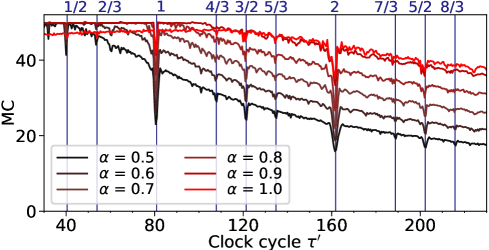
Figure 7: Influence of the parameter $\alpha$ of the linear model of Eq. (12) on the linear memory capacity. All other parameters are as in table 1. The numerical simulations in the main part of this report were obtained with $\alpha=0.9$.

Figure 7 shows the memory capacity as a function of the clock cycle $\tau^{\prime}$ for different $\alpha$. The effect is visible for a large range of values. In the paper, we have used $\alpha=0.9$, corresponding to the highest capacity out of the tested ones.

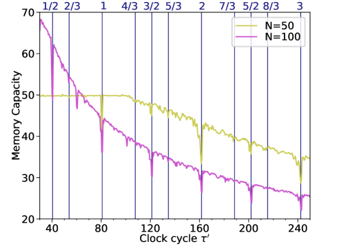
Figure 8: Influence of the parameter $N$ for the linear model of Eq. (12) on the linear memory capacity. All other parameters are as in table 1. The numerical simulations in the main part of this report were obtained with $N=50$.

Figure 8 shows the memory capacity as a function of the clock cycle $\tau^{\prime}$ for two different numbers of virtual nodes $N=50$ and $N=100$. Since the time per virtual node is $\theta=\tau^{\prime}/N$, it ranges between $0.6$ and $5.0$ in the case $N=50$ and between $0.3$ and $2.5$ in the case $N=100$. In both cases The effect is visible. In the paper, we have used $N=50$.

References

- [1] H. Jaeger, The “echo state” approach to analysing and training recurrent neural networks, Ger. Natl. Res. Cent. Inf. Technol. GMD Tech. Rep. 148.
- [2] W. Maass, T. Natschläger, H. Markam, Real-time computing without stable states: A new framework for neural computation based on perturbations, Neural Comput. 14 (11) (2002) 2531–2560.
- [3] G. Van der Sande, D. Brunner, M. C. Soriano, Advances in photonic reservoir computing, Nanophotonics 6 (3) (2017) 561. doi:https://doi.org/10.1515/nanoph-2016-0132.
- [4] D. Brunner, B. Penkovsky, B. A. Marquez, M. Jacquot, I. Fischer, L. Larger, Tutorial: Photonic neural networks in delay systems, J. Appl. Phys. 124 (15) (2018) 152004. doi:10.1063/1.5042342.
- [5] H. Jaeger, H. Haas, Harnessing Nonlinearity: Predicting Chaotic Systems and Saving Energy in Wireless Communication, Science (80-. ). 304 (5667) (2004) 78–80. doi:10.1126/SCIENCE.1091277.
-
[6]
D. Verstraeten, B. Schrauwen, D. Stroobandt, J. Van Campenhout,
Isolated
word recognition with the Liquid State Machine: a case study, Inf. Process.
Lett. 95 (6) (2005) 521–528.
doi:10.1016/J.IPL.2005.05.019.
URL https://www.sciencedirect.com/science/article/pii/S0020019005001523?via{%}3Dihub -
[7]
D. Verstraeten, B. Schrauwen, D. Stroobandt,
Reservoir-based
techniques for speech recognition, in: 2006 IEEE Int. Jt. Conf. Neural
Netw. Proc., IEEE, 2006, pp. 1050–1053.
doi:10.1109/IJCNN.2006.246804.
URL http://ieeexplore.ieee.org/document/1716215/ - [8] A. Argyris, J. Bueno, I. Fischer, Photonic machine learning implementation for signal recovery in optical communications, Sci. Rep. 8 (8487) (2018) 1–13. doi:10.1038/s41598-018-26927-y.
- [9] J. Pathak, B. Hunt, M. Girvan, Z. Lu, E. Ott, Model-Free Prediction of Large Spatiotemporally Chaotic Systems from Data: A Reservoir Computing Approach, Phys. Rev. Lett. 120 (2) (2018) 24102. doi:10.1103/physrevlett.120.024102.
- [10] H. Jaeger, Short Term Memory in Echo State Networks, Ger. Natl. Res. Cent. Inf. Technol. GMD Tech. Rep. 152.
- [11] T. Lymburn, A. Khor, T. Stemler, D. C. Corrẽa, M. Small, T. Jüngling, Consistency in echo-state networks, Chaos 29.
-
[12]
L. Appeltant, M. Soriano, G. Van der Sande, J. Danckaert, S. Massar,
J. Dambre, B. Schrauwen, C. Mirasso, I. Fischer,
Information processing
using a single dynamical node as complex system, Nat. Commun. 2 (1) (2011)
468.
doi:10.1038/ncomms1476.
URL http://www.nature.com/articles/ncomms1476 - [13] A. Röhm, K. Lüdge, Multiplexed networks: reservoir computing with virtual and real nodes, J. Phys. Commun. 2 (2018) 85007. doi:10.1088/2399-6528/aad56d.
- [14] T. Erneux, Applied Delay Differential Equations, Vol. 3 of Surveys and Tutorials in the Applied Mathematical Sciences, Springer, 2009.
-
[15]
T. Erneux, J. Javaloyes, M. Wolfrum, S. Yanchuk,
Introduction to Focus
Issue: Time-delay dynamics, Chaos An Interdiscip. J. Nonlinear Sci. 27 (11)
(2017) 114201.
doi:10.1063/1.5011354.
URL http://aip.scitation.org/doi/10.1063/1.5011354 -
[16]
S. Yanchuk, G. Giacomelli,
Spatio-temporal
phenomena in complex systems with time delays, J. Phys. A Math. Theor.
50 (10) (2017) 103001.
doi:10.1088/1751-8121/50/10/103001.
URL http://stacks.iop.org/1751-8121/50/i=10/a=103001?key=crossref.f760c062e912b820ac69c9174ac61305 - [17] D. Brunner, M. C. Soriano, C. R. Mirasso, I. Fischer, Parallel photonic information processing at gigabyte per second data rates using transient states, Nat. Commun. 2.
-
[18]
L. Larger, M. C. Soriano, D. Brunner, L. Appeltant, J. M. Gutierrez,
L. Pesquera, C. R. Mirasso, I. Fischer,
Photonic
information processing beyond Turing: an optoelectronic implementation of
reservoir computing, Opt. Express 20 (3) (2012) 3241–3249.
doi:10.1364/OE.20.003241.
URL http://www.opticsexpress.org/abstract.cfm?URI=oe-20-3-3241 - [19] Y. Kuriki, J. Nakayama, K. Takano, A. Uchida, Impact of input mask signals on delay-based photonic reservoir computing with semiconductor lasers, Optics Express 26.
-
[20]
N. F. Rulkov, M. M. Sushchik, L. S. Tsimring, H. D. I. Abarbanel,
Generalized
synchronization of chaos in directionally coupled chaotic systems, Phys.
Rev. E 51 (1995) 980–994.
doi:10.1103/PhysRevE.51.980.
URL https://link.aps.org/doi/10.1103/PhysRevE.51.980 - [21] A. Pikovsky, M. Rosenblum, J. Kurths, Synchronization: A universal concept in nonlinear science, Cambridge University Press, 2001.
- [22] J. Hale, S. Verduyn Lunel, An Introduction to Functional Differential Equations, Vol. 99, 1993.
- [23] H. Smith, An Introduction to Delay Differential Equations with Applications to the Life Sciences, Vol. 57, 2010. doi:10.1007/978-1-4419-7646-8.
- [24] J. Schumacher, H. Toutounji, G. Pipa, An analytical approach to single node delay-coupled reservoir computingdoi:10.1007/978-3-642-40728-4_4.
- [25] J. Schumacher, H. Toutounji, G. Pipa, An Analytical Approach to Single Node Delay-Coupled Reservoir Computing, Conference: 23rd International Conference on Artificial Neural Networks (2013). doi:10.1007/978-3-642-40728-4_4.
- [26] Y. Paquot, F. Duport, A. Smerieri, J. Dambre, B. Schrauwen, M. Haelterman, S. Massar, Optoelectronic Reservoir Computing, Sci. Rep. 2 (287). doi:10.1038/srep00287.
- [27] A. F. Atiya, A. G. Parlos, New Results on Recurrent Network Training: Unifying the Algorithms and Accelerating Convergence, IEEE Trans. Neural Networks 11 (3).
- [28] A. S. Weigend, N. A. Gershenfeld, Results of the time series prediction competition at the santa fe institute, in: IEEE International Conference on Neural Networks, 1993, pp. 1786–1793 vol.3. doi:10.1109/ICNN.1993.298828.
-
[29]
L. Larger, A. Baylón-Fuentes, R. Martinenghi, V. S. Udaltsov, Y. K. Chembo,
M. Jacquot,
High-speed photonic
reservoir computing using a time-delay-based architecture: Million words per
second classification, Phys. Rev. X 7 (2017) 011015.
doi:10.1103/PhysRevX.7.011015.
URL https://link.aps.org/doi/10.1103/PhysRevX.7.011015 - [30] S. Haykin, Adaptive filter theory, 3rd Edition, Prentice Hall, 1995.
- [31] J. Dambre, D. Verstraeten, B. Schrauwen, S. Massar, Information processing capacity of dynamical systems, Sci. Rep. 2 (2012) 514. doi:10.1038/srep00514.