Study of the superconducting to normal transition

Abstract

A model, based on classical mechanics and thermodynamics and valid for all superconductors, is devised to investigate the properties of the current-driven, superconducting to normal transition. This process is shown to be reversible. An original derivation of the BCS variational procedure is given. Two different critical temperatures are introduced. The temperature dependence of the critical current is worked out and found to agree with observation. The peculiar transport properties of high-$T_{c}$ compounds in the normal state and old magnetoelastic data are also interpreted within this framework. A novel experiment is proposed to check the relevance of this analysis to high-$T_{c}$ superconductivity.

I Introduction

Shortly after the discovery of superconductivity, it was realized that applying a growing magnetic fieldpar ; tin ; sch ; gen $H$ turns superconducting electrons into normal ones at a critical value $H=H_{c}$. Besides, this process has been characterized as a reversible first order transition, i.e. decreasing $H$ from $H_{c}$ down to $0$ brings normal electrons back to the superconducting state. However, this experimental procedure suffers from several drawbacks, when scrutinized from a thermodynamical standpoint :

• because all experiments have been made so farpar ; tin ; sch ; gen ; and ; rul1 ; laa ; sug ; rul ; gri at fixed temperature $T$, the heat exchanged during the transition remains unknown. Likewise, since nobody bothered to measure the work performed by $H$, the binding energy of the superconducting phase with respect to the normal one $E_{b}$ could not be assessed with help of the first law of thermodynamics. Meanwhile the formula $E_{b}=\mu_{0}H_{c}^{2}/2$ was assumedgor , with $\mu_{0}$ being the magnetic permeability of vacuum, and became eventually ubiquitous in textbookspar ; tin ; sch ; gen . Unfortunately, a numerical application in case of $Al$ turns out to underestimatesz2 by ten orders of magnitude the $E_{b}$ value, deduced from the BCS theorybcs ;

• due to the Meissner effectsz2 and the finite ac conductivitysch in the superconducting state, the current density is spatially inhomogeneoussz2 ; sz1 ; sz3 and there is no one-to-one correspondence between the external magnetic field and the current distribution inside the sample, so that qualitative information only can be achieved from $H$ mediated experimentspar ; tin ; sch ; gen ; and ; rul1 ; laa ; sug ; rul ; gri . At last, letting high $T_{c}$ compounds go normal requires a huge, often unpractical magnetic fieldand ; rul1 ; laa ; sug ; rul ; gri .

Consequently, despite countless published $H_{c}$ datapar ; tin ; sch ; gen ; and ; rul1 ; laa ; sug ; rul ; gri ; ande ; arm , there is still no theory of the superconducting to normal transition, apart from the phenomenologicalpar ; tin ; sch ; gen approach, based on the grossly wrong assumption $E_{b}=\mu_{0}H_{c}^{2}/2$. Thus the purpose of the present article is to design one, valid for both high and low $T_{c}$ superconductors, as well. Accordingly, since it has been argued recentlysz4 that feeding a growing current into a superconductor drives continuously the superconducting phase to the normal one, this article will focus on a theoretical account of the current-driven, superconducting to normal transition. Such an experimental procedure enables one to dodge all of the shortcomings mentioned above, in particular because reliable data for the critical current are available in all superconductors, including those for which $H_{c}$ is so large that it cannot be reached experimentally. Furthermore it allows for a quantitative treatment, unlike the $H$ mediated procedure. At last, since the current, carried by the superconducting electrons, plays a paramount role hereafter, it is worth mentioning an original viewkoi1 , which establishes the common significance of the persistent currentskoi2 and Josephson effectjos .

The purpose of this work is then twofold :

• this transition will be studied with help of Newton’s law and thermodynamics;

• the resulting findings will be taken advantage of to shed light into the transport properties of high $T_{c}$ compounds in the controversialande ; arm ; zan ; led $T>T_{c}$ range and the magneto-elastic behaviour, observed in elementary superconductorsols ; ols2 for $T\leq T_{c}$.

The outline is as follows : the electrodynamical and thermodynamical properties of the superconducting to normal transition are worked out in sections $2,3$, respectively; a new derivation of the BCS calculation is given in section $4$, which enables us to define two critical temperatures and to reckon the $T$ dependent critical current; this analysis is further applied to investigate the transport properties of high-$T_{c}$ compounds for $T>T_{c}$, in section $5$; magneto-elastic dataols ; ols2 are discussed in section $6$; the results of this work are summarized in the conclusion.

II Electrodynamical discussion

As done previouslysz4 ; sz2 ; sz1 ; sz3 , our analysis will proceed within the two-fluid model. Accordingly, the conduction electrons make up a homogeneous mixture of normal and superconducting electrons, in concentration $c_{n},c_{s}$, respectively. The normal electrons behave like a Fermi gasash , characterised by $T$ and the Fermi energy $E_{F}$. The Helmholz free energy of independent electrons per unit volume $F_{n}$ and $E_{F}$ are relatedash ; lan by $E_{F}=\frac{\partial F_{n}}{\partial c_{n}}$. By contrast, the superconducting electrons are organised as a many bound electron statesz4 of eigenenergy per unit volume $\mathcal{E}_{s}(c_{s})$, such that its chemical potential reads $\mu=\frac{\partial\mathcal{E}_{s}}{\partial c_{s}}$. Gibbs and Duhem’s lawlan entails that the thermal equilibrium is characterised by

$$E_{F}(T,c_{n}(T))=\mu(c_{s}(T))\quad,$$ (1)

with $c_{0}=c_{n}(T)+c_{s}(T)$ and $c_{0}$ being the concentration of conduction electrons.

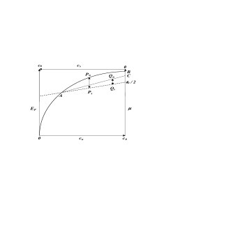
Figure 1: schematic plots of $E_{F}(T<T_{c},c_{n})$ and $\mu(c_{s})$ as solid and dashed lines, respectively; the origin $E_{F}=\mu=0$ is set at the bottom of the conduction band; the tiny difference $E_{F}(T,c_{n})-\mu(c_{0}-c_{n})$ has been hugely magnified for the reader’s convenience; the crossing point $A$ between the solid and dashed lines represents the electron system in thermal equilibrium at $T,T_{*}$, according to Eq.(1); the isothermal process, addressed in sections $2,3$ is pictured by the $P_{n},P_{s}$ pair, whereas the dotted line and the $Q_{n},Q_{s}$ pair illustrate the adiabatic process, discussed in section $5$

Consider then a superconducting material of cylindrical shape, characterized by its symmetry axis $z$ and radius $r_{0}$ in a cylindrical frame with coordinates ($r,\theta,z$) and flown through, along the $z$ direction, by a time dependent current $I(t)=\pi r_{0}^{2}j(t)$, with $j(t)$ being a uniform current density. The analysis of an isothermal, current-driven, superconducting to normal transition, outlined elsewheresz4 , will be developed below with $j(t)=\gamma t,\gamma>0$. Accordingly, the initial state of the whole electron system is defined as $j(0)=0,c_{n}=c_{n}(T),c_{s}=c_{s}(T)$ (see $A$ in Fig.1). As $j(t)$ increases at constant $T$, the electron system shifts away from the equilibrium position in $A$ : the Fermi gas, represented by $P_{n}$ in Fig.1, moves, along the solid line, towards $B$, corresponding to the normal state $c_{n}=c_{0}$, while the superconducting electrons, represented by $P_{s}$, go, along the dashed line, towards the point characterizedsz4 by $\mu(c_{s}=0)=\frac{\varepsilon_{c}}{2}$ ($\varepsilon_{c}$ refers to the Cooper pair energycooper ). As this process will be shown to be reversible, the pair $P_{n},P_{s}$, will shift back along the solid and dashed lines and will eventually merge into $A$, if $j$ is brought back down to $0$. The rest of section $1$ below deals with a detailed, quantitative account of the isothermal process, outlined above and illustrated in Fig.1.

Due to $\gamma=\frac{dj}{dt}\neq 0$, Newton’s law readssz4 ; sz2 ; sz1 ; sz3 for the normal and superconducting current densities $j_{n}(t)$, $j_{s}(t)$ ($\Rightarrow j=j_{n}+j_{s}$; note that $j_{s}$ is also referredkoi1 to as a collective mode current)

$$\tau_{n}\frac{dj_{n}}{dt}=\sigma_{n}E-j_{n}\quad,\quad\tau_{s}\frac{dj_{s}}{dt}=\sigma_{s}\left(E-E_{s\rightarrow n}\right)-j_{s}.$$ (2)

$E$ and $\tau_{n},\tau_{s}$ are, respectively, the applied electric field and the decay times of $j_{n},j_{s}$, due to friction with the lattice, responsible for Ohm’s law, whereas $\sigma_{n}=\frac{c_{n}e^{2}\tau_{n}}{m},\sigma_{s}=\frac{c_{s}e^{2}\tau_{s}}{m}$ stand for the normal and superconducting conductivitiessz1 ; sz3 ($\tau_{n}<<\tau_{s}\Rightarrow\sigma_{n}<<\sigma_{s}$) and $m,e$ refer to the effectiveash mass and charge of an electron. Moreover $\tau_{s}$ being finite has been demonstrated elsewheresz3 and shownsz4 furthermore to be consistent with observation of persistent currents at $E=0$. The effective field $E_{s\rightarrow n}$ is defined with respect to $f_{s\rightarrow n}=c_{s}eE_{s\rightarrow n}$, the interelectron force, which turns superconducting electrons into normal ones. The resulting $f_{s\rightarrow n}$ is mediated by the interelectron coupling, also responsible for the binding energy of the superconducting electrons, i.e. $E_{b}>0$. Actually $E_{s\rightarrow n}$ was neglected in previoussz4 ; sz2 ; sz1 ; sz3 works ($\Rightarrow j_{s}\approx\sigma_{s}E$). But, as it will appear below that $\left|\frac{E_{s\rightarrow n}}{E}\right|<<1$, such an approximation was fully vindicated.

During the elementary time-duration $\delta t$, superconducting electrons in concentration $\delta c_{s}$, moving at the mass center velocitysz4 ; sz2 ; sz1 ; sz3 $v_{s}$ ($\Rightarrow v_{s}=\frac{j_{s}}{c_{s}e}$), are driven normal at vanishing velocity by $f_{s\rightarrow n}$, which corresponds to a momentum variation per unit volume of $\delta p=-m\delta c_{s}v_{s}$. Thence $f_{s\rightarrow n}$ is inferred from Newton’s law to read

$$f_{s\rightarrow n}=\frac{\delta p}{\delta t}=-\frac{m\dot{c}_{s}}{c_{s}e}j_{s}\Rightarrow E_{s\rightarrow n}=-\frac{m\dot{c}_{s}}{(c_{s}e)^{2}}j_{s}\quad,$$ (3)

with $\dot{c}_{s}=\frac{dc_{s}}{dt}$. Then combining Eqs.(2,3), while recalling that the inertial force $\propto\frac{dj_{s}}{dt}$ is negligiblesz2 ; sz1 , yields

$$\begin{array}[]{c}E=\frac{j_{n}}{\sigma_{n}}=\frac{j_{s}}{\sigma_{s}}+E_{s\rightarrow n}\Rightarrow\frac{j_{n}}{\sigma_{n}}=\frac{j_{s}}{\sigma_{s}^{*}}=\frac{j}{\sigma_{n}+\sigma_{s}^{*}}\\ \sigma_{s}^{*}=\frac{\sigma_{s}}{1-\tau_{s}\frac{\dot{c}_{s}}{c_{s}}}\end{array}\quad.$$ (4)

Eq.(4) conveys the same meaning as Ohm’s law, written for $j_{n},j_{s}$ flowing parallel to each other, except for the effective conductivity $\sigma_{s}^{*}$ showing up instead of $\sigma_{s}$.

The elementary work $\delta W$, needed for one superconducting electron, moving with velocity $v_{s}$, to go normal with vanishing velocity, is reckoned to be equal to $\delta W=\frac{mv_{s}^{2}}{2}=\frac{m}{2}\left(\frac{j_{s}}{c_{s}e}\right)^{2}$, thanks to the kinetic energy theorem. On the other hand, for an isothermal process, $\delta W$ is also equal to the difference of free energylan between the superconducting and normal states, which leads thence to the identitylan $\delta W=\frac{\partial F_{n}}{\partial c_{n}}-\frac{\partial\mathcal{E}_{s}}{\partial c_{s}}=E_{F}(T,c_{n})-\mu(c_{s})$. Consequently, $j_{s}$ reads finally

$$j_{s}(c_{s})=c_{s}e\sqrt{\frac{2}{m}\left(E_{F}(T,c_{0}-c_{s})-\mu(c_{s})\right)}\quad.$$ (5)

Note that, unlike the normal current $j_{n}=\sigma_{n}E$, $j_{s}$ is independent from the external field $E$ and depends only on the concentration of bound electrons $c_{s}$.

Eq.(4) can now be recast as an ordinary differential equation of first order for the unknown $c_{s}(j)$

$$\gamma\frac{d\log c_{s}}{dj}=\frac{\frac{c_{s}}{c_{n}\tau_{n}}\left(\frac{j}{j_{s}(c_{s})}-1\right)-\frac{1}{\tau_{s}}}{\frac{c_{s}}{c_{n}}\left(\frac{j}{j_{s}(c_{s})}-1\right)-1}\quad,$$ (6)

with $c_{n}=c_{0}-c_{s}$ and $j_{s}$ given by Eq.(5).

For $j$ increasing from $0$, $c_{s}$ decreases from $c_{s}(T)$, while $E_{F}-\mu$ increases from $0$, proportionally to the length of the arrow linking $P_{n},P_{s}$ in Fig.1. In addition, since $j_{s}$ will eventually vanish for $c_{s}\rightarrow 0$, as inferred from Eq.(5), $j_{s}$ is bound to rise from $j_{s}=0$ at $A$ up to a maximum $j_{s}(c_{m})$ at $c_{m}(T)<c_{s}(T)$ defined by $\frac{dj_{s}}{dc_{s}}(c_{m})=0$. In order to solve Eq.(6), $E_{F}-\mu$ will be replaced by its Taylor’s expansion at first order with respect to $c_{s}-c_{s}(T)$

$$\frac{e^{2}}{m}\left(E_{F}-\mu\right)=\beta\left(c_{s}(T)-c_{s}\right)\Rightarrow c_{m}=\frac{2}{3}c_{s}(T)\quad,$$ (7)

with $\beta=\frac{e^{2}}{m}\left(\frac{\partial E_{F}}{\partial c_{n}}(c_{n}(T))+\frac{\partial\mu}{\partial c_{s}}(c_{s}(T))\right)$. Thus Eq.(6) has been integrated with $c_{0}=10^{28}/m^{3},c_{s}(T)=.1c_{0},\tau_{s}=10^{-9}s,\tau_{n}=10^{-4}\tau_{s},\beta=10^{-65}A^{2}\times m^{5}$ and initial condition $c_{s}(j=0)=c_{s}(T)$. The resulting data $c_{s}(j),\sigma_{e}(j)$ ($\sigma_{e}=\sigma_{n}+\sigma_{s}^{*}$ refers to the effective conductivity) have been plotted in Figs.2,3, corresponding to $j\leq j_{m}$ or $j>j_{m}$, respectively, with $j_{m}$ defined by $j_{m}=j_{s}(c_{m})$.

For $j\leq j_{m}$, there is $\tau_{s}\left|\frac{\dot{c}_{s}}{c_{s}}\right|<<1$, so that Eq.(4) yields $\sigma_{s}^{*}\approx\sigma_{s}$ and Eq.(6) reduces to

$$\frac{j_{s}(c_{s})}{j}=1+\frac{\sigma_{n}}{\sigma_{s}}=1+\frac{\tau_{n}}{\tau_{s}}\left(\frac{c_{0}}{c_{s}}-1\right)\quad.$$ (8)

Likewise, Eq.(8) implies $j_{s}\approx\sigma_{s}E\Rightarrow\left|\frac{E_{s\rightarrow n}}{E}\right|<<1$, which confirms the validity of a previous assumption. As $\gamma$ does not show up in Eq.(8), there is a one-to-one correspondence between $j$ and $c_{s}$, as seen in Fig.2. Moreover, $\tau_{n}<<\tau_{s}$ entails that $j_{s}\approx j$, so that the $c_{s}(j),\sigma_{e}(j)$ plots cannot be distinguished from each other. Note that $\frac{dc_{s}}{dj}(j=0)=0$, while $\left|\frac{dc_{s}}{dj}\right|$ becomes very large for $j\rightarrow j_{m}$.

Figure 2: plots of $c_{s}(j),\sigma_{e}(j)$ for $j\leq j_{m}$, as a solid line; the results have been found to be independent from $\gamma$ in accordance with Eq.(8)

However, when $j$ keeps growing beyond $j_{m}$, $j_{s}\approx j$ is no longer valid because of $j_{s}\leq j_{m}<j$. Consequently, as seen in Fig.3 , $c_{s}(j)$, obtained by integrating Eq.(6) for $j>j_{m}$, falls steeply from $c_{s}(j_{m})=c_{m}$ down to $0$, and $\sigma_{e}$ sinks by the ratio $\frac{c_{s}(T)\tau_{s}}{c_{0}\tau_{n}}=10^{3}$ from $\sigma_{e}(T)\approx\sigma_{s}(T)$ down to $\sigma_{e}(T_{c})=\frac{c_{0}e^{2}\tau_{n}}{m}$, typical of the normal metal. Meanwhile $j$ undergoes a tiny increase from $j_{m}$ up to $j_{M}$, with $j_{M}$ being weakly $\gamma$ dependent, i.e. $j_{M}/j_{m}-1\approx 10^{-7},10^{-8}$ for $\gamma=2\times 10^{9},2\times 10^{7}A/(m^{2}\times s)$, respectively (see Fig.3). Finally, due to $j_{M}\approx j_{m}=j_{s}(c_{m})$, $j_{M}(T<T_{c})$ reads

$$j_{M}=ec_{m}(T)\sqrt{\frac{2}{m}\left(E_{F}\left(T,c_{0}-c_{m}(T)\right)-\mu(c_{m}(T))\right)}\quad.$$

Integrating Eq.(6) from $j=j_{M}$ down to $j=0$ with the initial condition $c_{s}=c_{s}(j_{M})\approx 0$, while keeping $\gamma$ unaltered, will produce the same solution $c_{s}(j)$, as displayed in Figs.2,3. This shows that the superconducting-normal transition is reversible and there is a one-to-one correspondence between $j$ and $c_{s}$, provided that $\gamma$ keeps the same value for $j$ increasing from $0$ up to $j_{M}$ or decreasing from $j_{M}$ down to $0$, as well. This property holds actually for any $j(t)$, such that $j(t)=j(t_{p}-t),\forall t\in\left[0,t_{p}/2\right]$, with $t_{p}$ taken such that $j(t_{p}/2)=j_{M}$.

Due to $j_{s}\approx j$ for $j<j_{m}$, measuring $\sigma_{e}(j)$ and the $j$ dependent London length, which gives accesssz1 ; sz3 to $c_{s}$, would enable one to chart $E_{F}(T,c_{n})-\mu(c_{s})$ with help of Eq.(5). Given the highest observed $j_{M}$ values, Eq.(5) provides the estimate $E_{F}(T,c_{n})-\mu(c_{s})<10^{-5}eV$. It is noticeable that the conductivity, decreasing by several orders of magnitude for $j\rightarrow j_{M}$, as seen above, and for $T\rightarrow T_{c}^{-}$, as discussed elsewheresz3 , is to be ascribed, in both cases, to $c_{s}$ decreasing very steeply down to $0$.

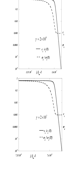
Figure 3: plots of $c_{s}(j),\sigma_{e}(j)$ for $j>j_{m}$, as a solid and dashed line, respectively; the calculation has been done for two values $\gamma=2\times 10^{7},2\times 10^{9}A/(m^{2}\times s)$

III Thermodynamical discussion

As recalled above, the work $W_{s\rightarrow n}$, performed by $f_{s\rightarrow n}$, whereby all of superconducting electrons are turned into normal ones via an isothermal processlan , is equal to the difference of free energy per unit volume $\Delta F$, between the normal and superconducting states. Due to the very definitions of $E_{F},\mu$, the work $W_{s\rightarrow n}$ is thence deduced to read

$$W_{s\rightarrow n}=\int_{0}^{c_{s}(T)}\left(E_{F}\left(T,c_{0}-u\right)-\mu\left(u\right)\right)du\quad.$$ (9)

In addition, Eq.(9) implies that $W_{s\rightarrow n}=-W_{n\rightarrow s}$, consistently with the reversible nature of the transition.

$W_{s\rightarrow n}$ can be also achieved alternatively by using the definition of $\Delta F=\Delta\mathcal{E}+T\Delta S$, with $\mathcal{E},S$ being, respectively, the total energy and entropy of the sample, i.e. including all of the lattice and electron degrees of freedom. $\Delta\mathcal{E},\Delta S$ will be calculated by working out the detailed thermal balance over the following trajectory : the sample is first taken at $T<T_{c}$ and heated up to $T_{c}$ with $j=0$. Hence, the associated $\Delta\mathcal{E}_{1},\Delta S_{1}$ read

$$\begin{array}[]{l}\Delta\mathcal{E}_{1}=\int_{T}^{T_{c}}\left(C_{\phi}(u)+C_{s}(u)\right)du\\ \Delta S_{1}=\int_{T}^{T_{c}}\left(C_{\phi}(u)+C_{s}(u)\right)\frac{du}{u}\end{array}\quad,$$ (10)

with $C_{\phi}(T),C_{s}(T)$ standing for the respective contributionsash to the specific heat of the phonons (Debye) and of the conduction electrons in the superconducting state; then let the sample be cooled down back to $T$, while being flown through by a current density $j\geq j_{M}(T)$, so that the sample remains normal down to $T$. The associated $\Delta\mathcal{E}_{2},\Delta S_{2}$ read then

$$\begin{array}[]{l}\Delta\mathcal{E}_{2}=\int_{T_{c}}^{T}\left(C_{\phi}(u)+C_{n}(u)\right)du\\ \Delta S_{2}=\int_{T_{c}}^{T}\left(C_{\phi}(u)+C_{n}(u)\right)\frac{du}{u}\end{array}\quad,$$ (11)

with $C_{n}(T)$ standing for the $T$ linear, specific heat of a Fermi gasash , which is known to be independent from $j$, like $C_{\phi}(T)$. At last, the searched expressions readgor

$$\begin{array}[]{l}E_{b}(T)=\Delta\mathcal{E}_{1}+\Delta\mathcal{E}_{2}=\int_{T}^{T_{c}}\left(C_{s}(u)-C_{n}(u)\right)du\\ W_{s\rightarrow n}(T)=\Delta\mathcal{E}_{1}+T\Delta\mathcal{S}_{1}+\Delta\mathcal{E}_{2}+T\Delta\mathcal{S}_{2}\\ \quad\quad\quad\quad\quad=\int_{T}^{T_{c}}\left(C_{s}(u)-C_{n}(u)\right)\left(1-\frac{T}{u}\right)du\end{array},$$ (12)

with $E_{b}(T)$ being the binding energy of the superconducting phase with respect to the normal one at $T$. Noteworthy is that the superconducting phase being stable ($\Leftrightarrow E_{b}(T)>0$) requires $C_{s}(T)>C_{n}(T)$ in Eq.(12), which is confirmed experimentallypar ; ash , i.e. $C_{s}(T_{c})\approx 3C_{n}(T_{c})$.

$W_{s\rightarrow n}$ can actually be measured directly by feeding a growing current $I(t)=\pi r_{0}^{2}\gamma t$ into the superconducting sample, from $t=0$ until $t=\frac{t_{p}}{2}$ with $I(\frac{t_{p}}{2})=\pi r_{0}^{2}j_{M}(T)$, so that the sample goes normal at $\frac{t_{p}}{2}$ (this is referred to as the Silsbee effectpar ). Then $I(t)$ is reduced, like $I(t)=\pi r_{0}^{2}\gamma\left(t_{p}-t\right)$, from $I\left(\frac{t_{p}}{2}\right)$ down to $I(t_{p})=0$. The work $W(t_{p})$, performed by the electric field $E$ from $t=0$ until $t=t_{p}$, reads then

$$\begin{array}[]{c}W(t_{p})=W_{1}+W_{2}\\ W_{1}=\int_{0}^{\frac{t_{p}}{2}}U(t)I(t)dt\quad,\quad W_{2}=\int^{t_{p}}_{\frac{t_{p}}{2}}U(t)I(t)dt\end{array}\quad,$$ (13)

with $U=El$ and $l$ being the measured voltage drop across the sample and its length, respectively. Moreover, owing to Eq.(4), $W_{1},W_{2}$ can be recast as

$$\begin{array}[]{c}\frac{W_{1}}{\pi r_{0}^{2}l}=\int_{0}^{\frac{t_{p}}{2}}\left(\frac{j_{n}^{2}}{\sigma_{n}}+\frac{j_{s}^{2}}{\sigma_{s}}+j_{s}E_{s\rightarrow n}\right)dt\\ \frac{W_{2}}{\pi r_{0}^{2}l}=\int_{\frac{t_{p}}{2}}^{t_{p}}\left(\frac{j_{n}^{2}}{\sigma_{n}}+\frac{j_{s}^{2}}{\sigma_{s}}+j_{s}E_{n\rightarrow s}\right)dt\end{array}\quad.$$ (14)

Likewise, recalling that $j_{n},\sigma_{n},j_{s},\sigma_{s}$ have been shown above to depend on $j$ only, if $\gamma$ is kept fixed, and furthermore

$$\begin{array}[]{c}W_{s\rightarrow n}=\int_{0}^{\frac{t_{p}}{2}}j_{s}E_{s\rightarrow n}dt\quad,\quad W_{n\rightarrow s}=\int_{\frac{t_{p}}{2}}^{t_{p}}j_{s}E_{n\rightarrow s}dt\\ W_{s\rightarrow n}=-W_{n\rightarrow s}\end{array}\quad,$$

enables us to recast $W_{1},W_{2}$ as

$$\begin{array}[]{c}\frac{W_{1}}{\pi r_{0}^{2}l}=Q_{1}+W_{s\rightarrow n}\quad,\quad\frac{W_{2}}{\pi r_{0}^{2}l}=Q_{1}-W_{s\rightarrow n}\\ Q_{1}=\int_{0}^{j_{M}(T)}\left(\frac{j_{n}^{2}}{\sigma_{n}}+\frac{j_{s}^{2}}{\sigma_{s}}\right)\frac{dj}{\gamma}\end{array}\quad,$$ (15)

with $Q_{1}$ expressing the Joule heat, releasedsz4 through process I per unit volume for $t\in\left[0,t_{p}/2\right]$. Finally it ensues from Eq.(15)

$$\frac{W_{1}-W_{2}}{2\pi r_{0}^{2}l}=\int_{T}^{T_{c}}\left(C_{s}(u)-C_{n}(u)\right)\left(1-\frac{T}{u}\right)du\quad.$$ (16)

The validity of Eq.(16) should be checked experimentally first in a superconducting material, for which accurate data are available for $C_{s},C_{n}$ and thence $T_{c}$ is lowash enough for $C_{s}>C_{\phi},C_{n}>C_{\phi}$. Accordingly, $Al$ ($T_{c}=1.19K$) might be a good candidate. In case of a successful test, Eq.(16) might then provide with a rather unique access to $C_{s}$ in high $T_{c}$ materials, for which the direct measurement of $C_{s}$ proves unreliablelor , due to $C_{s}<<C_{\phi}$. Note that $C_{n}$ can always be measured at low $T$ by feeding into the sample a current density $j>j_{M}(T)$, whereby the sample goes normal even at $T<T_{c}$, because $C_{n}$ is $j$ independent, unlike $C_{s}$, and extrapolated further to higher $T$, by taking advantage of its $T$ linear behaviourash .

Although the superconducting to normal transition and ice melting into water are both first order processes, they differ in two respects :

• the role of the latent heat, typical of all usual first order transitions (melting or vaporisation), is played here by the latent work $W_{s\rightarrow n}$, because the superconducting-normal transition is controlled by current rather than by temperature;

• ice and water are separated by a clear-cut interface, whereas the mixture of superconducting and normal electrons is homogeneous. Consequently, the chemical potentials of ice and water remain uniquely defined all over the melting process, while $E_{F},\mu$ vary continuously with $c_{s}\in\left[0,c_{s}(T<T_{c})\right]$.

IV Critical current

As shown elsewheresz4 , the bound electron current $j_{s}$ will turn out to be persistent, only if the necessary condition $\sigma_{s}+\sigma_{J}>0$, with $\sigma_{J}<0$ being the conductivity characterising process II of the Joule effect, is fulfilled. It conveys the physical meaning that the negative Joule heat, released via the anomalous process II, typical of superconductors, should prevail over the positive one, stemming from the regular process I. Since $\sigma_{J}$ readssz4 as $\sigma_{J}=-\frac{(ev)^{2}\tau_{s}}{\left|\frac{\partial\mu}{\partial c_{s}}\right|}$ with $mv^{2}\approx 1eV$, the inequality $\sigma_{s}+\sigma_{J}>0$ can be recast as

$$r(c_{s})=\frac{c_{s}}{mv^{2}}\left|\frac{\partial\mu}{\partial c_{s}}\right|>1\quad.$$ (17)

As it will appear below that $\frac{\partial\mu}{\partial c_{s}}$ remains finite for $c_{s}\rightarrow 0$, the inequality (17) is bound not to hold any more for $c_{s}<c_{c}$ with the critical concentration $c_{c}$ defined by $r(c_{c})=1$. To proceed further, $c_{c}$ must be assessed, which requires to reckon $\frac{\partial\mu}{\partial c_{s}}$. The only practical tool for this purpose is the BCS schemebcs , but for some reason to become clear below, we shall refrain from using it, and rather develope our own procedure.

Thus let us consider a three-dimensional crystal containing $N$ sites and $2n$ itinerant electrons with $N>>1,n>>1$ ($\Rightarrow c_{s}=2n/N$). These electrons of spin $\sigma=\pm 1/2$ populate a single band, accomodating at most two electrons per site ($\Rightarrow n\leq N$). The independent electron motion is described, in reciprocal space, by the Hamiltonian $H_{d}$

$$H_{d}=\sum_{k,\sigma}\varepsilon(k)c^{+}_{k,\sigma}c_{k,\sigma}\quad,$$ (18)

for which $\varepsilon(k),k$ are the one-electron, spin-independent energy ($\Rightarrow\varepsilon(k)=\varepsilon(-k)$) and a vector of the Brillouin zone, respectively, and the sum over $k$ is to be carried out over the whole Brillouin zone. Then $c^{+}_{k,\sigma},c_{k,\sigma}$ are one-electron creation and annihilation operators on the Bloch state $\left|k,\sigma\right\rangle$

$$\left|k,\sigma\right\rangle=c^{+}_{k,\sigma}\left|0\right\rangle\quad,\quad\left|0\right\rangle=c_{k,\sigma}\left|k,\sigma\right\rangle\quad,$$

with $\left|0\right\rangle$ being the no electron state. They enable us to introduce the two-electron creation and annihilation operatorsbcs ; cooper ; ja1 $b^{+}_{K,k}=c^{+}_{k,+}c^{+}_{K-k,-},b_{K,k}=c_{K-k,-}c_{k,+}$, which operate on hard-core bosons and thence do not fulfill the boson commutation rules. The interacting electron motion is governed by a truncated Hubbard Hamiltonian $H_{K}$, used previouslybcs ; ja1

$$H_{K}=\sum_{k}\varepsilon(K,k)b^{+}_{K,k}b_{K,k}+\frac{U}{N}\sum_{k,k^{\prime}}b^{+}_{K,k}b_{K,k^{\prime}}\quad,$$ (19)

with $\varepsilon(K,k)=\varepsilon(k)+\varepsilon(K-k)$ and $U$ being the Hubbard coupling constant. Unlike previous authorstin ; sch ; bcs ; cooper , we shall consider both cases $U>0,U<0$.

The eigenstate of the Schrödinger equation, pertaining to a single bound pair, $\left(H_{K}-\varepsilon_{c}(K)\right)\varphi_{c}=0$, is known as the Cooper paircooper state $\varphi_{c}=\sum_{k}\frac{b^{+}_{K,k}}{\varepsilon_{c}(K)-\varepsilon(K,k)}\left|0\right\rangle$, with the eigenenergy $\varepsilon_{c}(K)$ being the solution of

$$\frac{1}{U}=\frac{1}{N}\sum_{k}\frac{1}{\varepsilon_{c}(K)-\varepsilon(K,k)}=\int_{-t_{K}}^{t_{K}}\frac{\rho_{K}(\varepsilon)}{\varepsilon_{c}(K)-\varepsilon}d\varepsilon.$$ (20)

$\pm t_{K}$ are the upper and lower bounds of the two-electron band, i.e. the maximum and minimum of $\varepsilon(K,k)$ over $k$, whereas $\rho_{K}(\varepsilon)$ is the corresponding two-electron density of states. For the sake of illustration, we shall solve Eq.(20) for $\rho_{K}(\varepsilon)=\frac{2}{\pi t_{K}}\sqrt{1-\left(\frac{\varepsilon}{t_{K}}\right)^{2}},t_{K}=t\cos\left(Ka/2\right)$, where $t,a$ are the one-electron bandwidth and the lattice parameter, respectively. The dispersion curves $\varepsilon_{c}(K)$ are given in Fig.4 for $U>0$ only, because it can be deduced from Eq.(20) and $\rho_{K}(\varepsilon)=\rho_{K}(-\varepsilon)$ that $\varepsilon_{c}(K,U)=-\varepsilon_{c}(K,-U)$. A remarkable feature is that $\varepsilon_{c}(K)\rightarrow t_{K}$, i.e. the upper bound of the two-electron band, for $U$ decreasing toward $t_{K}/2$, so that there is no Cooper pair solution for $U<t_{K}/2$ (accordingly, the dashed curve is no longer defined in Fig.4 for $\frac{Ka}{\pi}<.13$), in marked contrast with the opposite conclusion reached elsewherecooper , that there is a Cooper pair, even for $U\rightarrow 0$. This discrepancy results from the three-dimensional Van Hove singularities, showing up at both two-electron band edges $\rho_{K}\left(\varepsilon\rightarrow\pm t_{K}\right)\propto\sqrt{t_{K}-\left|\varepsilon\right|}$, unlike the two-electron density of states, used previouslycooper , which displayed no such singularity.

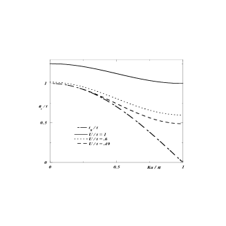
Figure 4: dispersion curves of $t_{K}$ as a dashed-dotted line and of $\varepsilon_{c}(K)$ as solid, dashed and dotted lines, associated with various $U$ values, respectively

$H_{K}$ operates within the Hilbert space $S_{K}$. A typical vector of its basis reads $\varphi=\prod_{i=1,..m}b^{+}_{K,k_{i}}\left|0\right\rangle$ with $m$ being any integer. We shall look for a variational approximation $\varphi_{v}$ of the singleja2 ; ja3 bound eigenstate of $H_{K}$ inside the subset $\left\{\varphi_{v}\right\}\subset S_{K}$, characterized by

$$\left\langle\varphi_{v}\right|b^{(+)}_{K,k}\left|\varphi_{v}\right\rangle=\left(n_{k}\left(1-n_{k}\right)\right)^{\alpha},\quad\forall\varphi_{v}\in\left\{\varphi_{v}\right\}\quad.$$

The real parameter $\alpha$ will be assigned shortly and $n_{k}=\left\langle\varphi_{v}\right|b^{+}_{K,k}b_{K,k}\left|\varphi_{v}\right\rangle$. The pair number operator $b^{+}_{K,k}b_{K,k}$ has two eigenvalues $0,1$, associated with $\left|0\right\rangle$ and $b^{+}_{K,k}\left|0\right\rangle$, respectively, so that $0\leq n_{k}\leq 1$ and $\sum_{k}n_{k}=n$. The energy of $\varphi_{v}$ per site reads

$$\begin{array}[]{c}\mathcal{E}=\frac{\left\langle\varphi_{v}\right|H_{K}\left|\varphi_{v}\right\rangle}{N}=\sum_{k}\varepsilon(K,k)\frac{n_{k}}{N}+U\Delta^{2}\\ \Delta=\sum_{k}\frac{\left(n_{k}\left(1-n_{k}\right)\right)^{\alpha}}{N}\end{array}\quad.$$

Hence minimising $\mathcal{E}$ ($\Rightarrow d\mathcal{E}=0$), under the constraint of $n$ kept constant ($\Rightarrow dn=0$), yields

$$\varepsilon(K,k)+2\alpha U\Delta\frac{1-2n_{k}}{\left(n_{k}\left(1-n_{k}\right)\right)^{1-\alpha}}=\lambda\quad,$$

with $\lambda=\frac{\partial\mathcal{E}}{\partial n_{k}},\forall k$ being a Lagrange multiplier, which implies that $\lambda=\frac{\partial\mathcal{E}}{\partial n}=2\mu(c_{s}=\frac{2n}{N})$. The $\alpha$ value will be assigned now by checking consistency with the Cooper pair properties in the limit $n\rightarrow 0\Rightarrow n_{k}\rightarrow 0\Rightarrow n_{k}\propto\left(2\mu-\varepsilon(K,k)\right)^{\frac{1}{\alpha-1}}$. Comparing with $n_{k}=\left\langle\varphi_{c}\right|b^{+}_{K,k}b_{K,k}\left|\varphi_{c}\right\rangle$ $\propto\left(\varepsilon_{c}(K)-\varepsilon(K,k)\right)^{-2}$, inferred from Eq.(20), yields finally $\alpha=1/2$ and $\varepsilon_{c}(K)=2\mu(c_{s}=0)$, a conclusion which had already been reached by an independent rationalesz4 . Hence, our variational procedure can be summarised, with help of notations introduced elsewheretin , as follows

$$\begin{array}[]{c}\tan 2\theta_{k}=\frac{2U\Delta}{2\mu-\varepsilon(K,k)}\quad,\quad n_{k}=\sin^{2}\theta_{k}\\ \Delta=\sum_{k}\frac{\sin 2\theta_{k}}{2N}=\int_{-t_{K}}^{t_{K}}\frac{\sin 2\theta(\varepsilon)}{2}\rho_{K}(\varepsilon)d\varepsilon\\ c_{s}=2\sum_{k}\frac{\sin^{2}\theta_{k}}{N}=2\int_{-t_{K}}^{t_{K}}\sin^{2}\theta(\varepsilon)\rho_{K}(\varepsilon)d\varepsilon\end{array}\quad,$$ (21)

with $0\leq\theta_{k}\leq\frac{\pi}{2}$. The formulae in Eqs.(21) are found to be identical to those of BCStin ; sch ; bcs . As an illustrative example, Eqs.(21) have been solved for $\mu(c_{s}),\Delta(c_{s})$ and $r(c_{s})$ defined by Eq.(17), with $U>0$ and $c_{s}<1$ electron per site, only, because it can be deduced from Eqs.(21) and $\rho_{K}(\varepsilon)=\rho_{K}(-\varepsilon)$ that $\mu(c_{s},U)=-\mu(c_{s},-U)$$=-\mu(2-c_{s},U)$. The results, presented in Fig.5, exhibit $\frac{\partial\mu}{\partial c_{s}}$ almost independent from $c_{s}$ and $\Delta(c_{s}\rightarrow 0)\propto\sqrt{c_{s}}$. An important inequality, holding for $U>0$ and $U<0$ as well, can be deduced from $\mu(c_{s},U)=-\mu(c_{s},-U)$ and Fig.5

$$U\frac{\partial\mu}{\partial c_{s}}<0\quad.$$ (22)

Note that for $K=\frac{\pi}{a}$, the two-electron band is dispersionless because of $t_{K=\frac{\pi}{a}}=0$. Then applying Eqs.(21) to the $K=\frac{\pi}{a}$ case gives $\Delta=\frac{\sin 2\theta}{2}$ and finally $\mu=\frac{U}{2}\left(1-c_{s}\right)$, the validity of which can be checked independently, because the $n$-pair, bound eigenstate of $H_{K=\frac{\pi}{a}}$ is knownja1 to read $\varphi=\sum_{i=1,..d}\frac{\varphi_{i}}{\sqrt{d}}$, with $d=\left(\begin{array}[]{c}N\\ n\end{array}\right)$, $\varphi_{i}=\prod_{l=1,..n}b^{+}_{\frac{\pi}{a},k_{i_{l}}}\left|0\right\rangle$ and the sum with respect to $i$ runs over all of $n$ pair combinations $\left\{b^{+}_{\frac{\pi}{a},k_{i_{1}}},...b^{+}_{\frac{\pi}{a},k_{i_{n}}}\right\}$, chosen among $N$ of available pairs. As each $\varphi_{i}$ contributes $\frac{n}{dN}(1-\frac{n}{N})U$ to $\mathcal{E}$, it can thence be inferred $\mathcal{E}=U\frac{c_{s}}{2}(1-\frac{c_{s}}{2})\Rightarrow\mu=\frac{\partial\mathcal{E}}{\partial c_{s}}=\frac{U}{2}\left(1-c_{s}\right)$, which is seen to be identical to the above result, deduced from Eqs.(21). At last, there is $U\frac{\partial\mu}{\partial c_{s}}=-U^{2}/2<0$ in accordance with inequality (22).

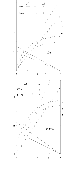
Figure 5: plots of $\mu(c_{s}),\Delta(c_{s}),r(c_{s})$ reckoned for $K=0,\frac{\pi}{2a}$; the solid and dotted lines and the triangles, which pertain to $\mu,r,\Delta$, respectively, have been calculated with $U/t=1$, whereas the dashed line and the $\times,+$ symbols, which refer to $\mu,r,\Delta$, respectively, have been calculated with $U/t=.6$; the $r$ data have been calculated with $mv^{2}=t/3$; $c_{s}=1$ corresponds to one electron per site

Combining Eq.(20) with Taylor’s expansions of $\sin 2\theta_{k}$, $\sin^{2}\theta_{k}$, worked out from Eqs.(21), up to $\Delta^{2}$ for $c_{s}\rightarrow 0\Rightarrow\Delta\rightarrow 0$, leads to

$$\begin{array}[]{l}\frac{1}{U}=\int_{-t_{K}}^{t_{K}}\frac{\rho_{K}(\varepsilon)}{\varepsilon_{c}(K)-\varepsilon}d\varepsilon\\ =\int_{-t_{K}}^{t_{K}}\left(1-2\left(\frac{U\Delta}{2\mu-\varepsilon}\right)^{2}\right)\frac{\rho_{K}(\varepsilon)}{2\mu-\varepsilon}d\varepsilon\\ \left(U\Delta\right)^{2}=\frac{c_{s}}{2\int_{-t_{K}}^{t_{K}}\frac{\rho_{K}(\varepsilon)}{\left(\varepsilon_{c}(K)-\varepsilon\right)^{2}}d\varepsilon}\end{array}\quad.$$

Subtracting the integrals equal to $1/U$ from each other, while taking advantage of $\mu(c_{s}\rightarrow 0)\rightarrow\varepsilon_{c}(K)/2$, gives in turn

$$\left(U\Delta\right)^{2}=\left(\frac{\varepsilon_{c}(K)}{2}-\mu\right)\frac{\int_{-t_{K}}^{t_{K}}\frac{\rho_{K}(\varepsilon)}{\left(\varepsilon_{c}(K)-\varepsilon\right)^{2}}d\varepsilon}{\int_{-t_{K}}^{t_{K}}\frac{\rho_{K}(\varepsilon)}{\left(\varepsilon_{c}(K)-\varepsilon\right)^{3}}d\varepsilon}\quad.$$

Equating both expressions of $\left(U\Delta\right)^{2}$ yields finally

$$\frac{\partial\mu}{\partial c_{s}}(K,c_{s}=0)=-\frac{\int_{-t_{K}}^{t_{K}}\frac{\rho_{K}(\varepsilon)}{\left(\varepsilon_{c}(K)-\varepsilon\right)^{3}}d\varepsilon}{2\left(\int_{-t_{K}}^{t_{K}}\frac{\rho_{K}(\varepsilon)}{\left(\varepsilon_{c}(K)-\varepsilon\right)^{2}}d\varepsilon\right)^{2}}\quad.$$

Note that $\left|\frac{\partial\mu}{\partial c_{s}}(K,c_{s}=0)\right|\rightarrow\infty$ for $U\rightarrow t_{K}/2$ and
$U\frac{\partial\mu}{\partial c_{s}}(K,c_{s}=0)<0$ in accordance with inequality (22).

With help of Fig.5, $c_{c}$, defined by $r(c_{c})=1$ in Eq.(17), can now be assigned, for $K=0$, to the values $.7,.54$, and for $K=\frac{\pi}{2a}$, to the values $.85,.6$, associated with $U/t=.6,1$, respectively. Noteworthy is that $\varphi_{v}$ will sustain persistent currents or not, according to whether $c_{s}>c_{c}$ or $c_{s}<c_{c}$, although $\varphi_{v}$ undergoes no qualitative change for $c_{s}=c_{c}$. Accordingly, it still obeys Eqs.(21) for $c_{s}>c_{c}$ and $c_{s}<c_{c}$, as well. Therefore, $\varphi_{v}(c_{s}<c_{c})$ will be referred to below, as the many-bound-electron, non-superconducting (MBENS) state. Moreover, applying Eq.(5) for $c_{s}=c_{c}$, while taking advantage of the Sommerfeld integralash and Eq.(1), yields the critical current density as

$$\begin{array}[]{l}j_{c}(T)=c_{c}e\sqrt{\frac{2}{m}\left(E_{F}\left(T,c_{0}-c_{c}\right)-\mu(c_{c})\right)}\\ \quad\quad\quad=\pi k_{B}ec_{c}\sqrt{\frac{\rho^{{}^{\prime}}(E_{F}^{*})}{3m\rho(E_{F}^{*})}\left(T_{*}^{2}-T^{2}\right)}\end{array}\quad,$$ (23)

with $E_{F}^{*}=E_{F}\left(T_{*},c_{0}-c_{c}\right)$. $k_{B},\rho(\varepsilon)$ designate Boltzmann’s constant and the one-electron density of states and $\rho^{{}^{\prime}}(\varepsilon)=\frac{d\rho}{d\varepsilon}$, while $T_{*}<T_{c}$ is defined by $E_{F}(T_{*},c_{0}-c_{c})=\mu(c_{c})\Rightarrow c_{s}(T_{*})=c_{c}$. The calculated behavior $j_{c}(T)\propto\sqrt{T_{*}^{2}-T^{2}}$, resulting from Eq.(23), is found to agree with observationtin ; sch ; gen ; ash . Consequently, the MBENS state and the superconducting one can be observed for $T_{*}<T<T_{c}$ and $T<T_{*}$, respectively. In a low $T_{c}$ metal such as $Sn$, $c_{s}$ has been shownsz3 to grow steeply from $c_{s}(T_{c})=0$ up to $c_{s}(T_{c}-.04K)\approx c_{s}(0)\Rightarrow T_{c}-T_{*}<.04K$, so that $T_{c},T_{*}$ are unlikely to be resolved experimentally from each other. However $T_{c}-T_{*}$ will be argued in the next section to be quite sizeable in high $T_{c}$ materials.

$\frac{\partial\mu}{\partial c_{s}}<0$ has been shownsz4 to be a prerequisite for persistent currents. Hence, the inequality 22 entails $U>0$. Besides, an additional setback of the assumptionbcs ; cooper $U<0\Rightarrow\frac{\partial\mu}{\partial c_{s}}>0$ is to preclude any thermal equilibrium for $T<T_{c}$. Here is a proof by contradiction. Let us assume that the BCS state is indeed in equilibrium at $T_{c}$, which implies $E_{F}(T_{c},c_{0})=\mu(c_{s}=0)$, because of $c_{s}(T_{c})=0,c_{n}(T_{c})=c_{0}$, in accordance with Eq.(1). When $T$ decreases from $T_{c}$ down to $0$, charge conservation $c_{0}=c_{n}(T)+c_{s}(T)$ entails

$$E_{F}(T)=E_{F}(T_{c})-\frac{c_{s}(T)}{\rho(E_{F}(T_{c}))},\quad\mu(T)=\mu(T_{c})+\frac{\partial\mu}{\partial c_{s}}c_{s}(T),$$

for which we have usedash $\frac{\partial E_{F}}{\partial c_{s}}=1/\rho(E_{F})$, while neglecting $\frac{\partial E_{F}}{k_{B}\partial T}\approx k_{B}T/E_{F}<<1$. Thus, $\frac{\partial\mu}{\partial c_{s}}>0$ implies $E_{F}(T)<E_{F}(T_{c})=\mu(T_{c})<\mu(T)$, so that the equilibrium condition $\mu(c_{s}(T))=E_{F}(T,c_{0}-c_{s}(T))$ in Eq.(1) cannot be fulfilled for any $T<T_{c}$. Q.E.D.

V High-$T_{c}$ compounds

Overdoped high $T_{c}$ compounds are knownand ; rul1 ; laa ; sug ; rul ; gri ; ande ; arm ; zan ; led to undergo, at $T_{c}$, a crossover from a superconducting state of type II, observed for $T<T_{c}$, to an ill-understood state, which sustains no persistent current, but the conduction properties of which differ yet markedly from those of usual metals up to $T>>T_{c}$ :

• contrary to the conductivity expected to be low, given the high doping rate $>.15$, it is observed to be large;

• the Hall coefficient is found to be $T$ dependent, which hints at a $T$ dependent carrier concentration, unlike what is observed in usual metals and alloys, behaving like a Fermi gasash with $T$ independent concentration.

Assuming $T_{c}=T_{*}$, both above mentioned features might be consistent with an electron system, comprising a Fermi gas and a MBENS state in respective concentration $c_{n}(T>T_{*}),c_{s}(T)$ and fulfilling Eq.(1) with $c_{0}=c_{n}(T)+c_{s}(T)$. As a matter of fact, $\tau_{s}>>\tau_{n}$ entailssz1 that the large conductivity is settled by the MBENS electrons only and the Hall coefficient, dominated by $j_{s}$, is $T$ dependent as is $c_{s}(T)$. The main virtue of such an assumption is that it lends itself to an experimental check, as shown below.

Consider a thermally isolated sample, flown through by $I(t)=\pi r_{0}^{2}j(t)$ with $j(t)=\gamma t$, and taken at $t=0$ in the thermal equilibrium state, represented by $A$ in Fig.1, i.e. $T(t=0)=T_{*},I(t=0)=0,c_{n}(t=0)=c_{n}(T_{*}),c_{s}(t=0)=c_{0}-c_{n}(T_{*})$. While $I(t)$ keeps growing, the bound electrons, pictured by $Q_{s}$ in Fig.1, are turned into independent ones, depicted by $Q_{n}$, as explained in section $2$. The experiment ends up at $t=t_{f}$, when $Q_{n}$, after traveling all along the dotted line, merges with $C$, referring to the normal state and thence characterized by $T(t_{f})=T_{f},c_{n}(t_{f})=c_{0},c_{s}(t_{f})=0$. Thus applying the first law of thermodynamics to this adiabatic process yields

$$\begin{array}[]{c}\int_{T_{*}}^{T_{f}}C_{\phi}(T)dT=Q_{1}+Q_{2}\quad,\quad Q_{2}=\int_{0}^{t_{f}}\frac{j_{s}^{2}(t)}{\sigma_{J}}dt\\ Q_{1}=\int_{0}^{t_{f}}\frac{U(t)}{l}j(t)dt=\int_{0}^{t_{f}}\left(\frac{j_{n}^{2}(t)}{\sigma_{n}}+\frac{j_{s}^{2}(t)}{\sigma_{s}}\right)dt\end{array},$$ (24)

where $Q_{1}>0,Q_{2}<0$ stand for the Joule heat released through processessz4 I and II, respectively, and $C_{n}(T>T_{*})<<C_{\phi}(T)$, $C_{s}(T>T_{*})<<C_{\phi}(T)$, $W_{s\rightarrow n}<<Q_{1}$ have been neglected. Derivating Eq.(24) with respect to $t$ gives finally

$$C_{\phi}(T)\dot{T}=\frac{U(t)}{l}j(t)+\frac{j_{s}^{2}}{\sigma_{J}}=\frac{j_{n}^{2}}{\sigma_{n}}+j_{s}^{2}\left(\frac{1}{\sigma_{s}}+\frac{1}{\sigma_{J}}\right),$$ (25)

with $\dot{T}=\frac{dT}{dt}$. Because of $\frac{1}{\sigma_{s}}+\frac{1}{\sigma_{J}}>0$, due to the very definition of $T_{*}$, we predict $\dot{T}>0\Rightarrow T_{f}>T_{*}$, with $\sigma_{J}<0\Rightarrow C_{\phi}(T)\dot{T}<\frac{U(t)}{l}j(t)$ . Despite $\dot{T}>0$ like in a usual metal, the latter inequality would rather read $C_{\phi}(T)\dot{T}=\frac{U(t)}{l}j(t)$, if the same experiment were carried out in a normal conductor. Conversely, would the experiment be performed at $T<T_{*}\Rightarrow\frac{1}{\sigma_{s}}+\frac{1}{\sigma_{J}}<0$, we should observesz4 $\dot{T}<0$, as remarked by De Gennes too (seegen footnote in p.18). Besides, the sign of $\dot{T}$ is independent of that of $\dot{I}$, because the Joule effect is irreversible. At last, due to the high doping rate, the local electron concentration is likely to display spatial fluctuations, which should eventually result into a sample, comprising both superconducting and MBENS domains. This case could be brought to experimental evidence by observing different values of $\dot{T}$ in Eq.(25), according to whether a dc ($\Rightarrow\dot{T}_{dc}$) or ac ($\Rightarrow\dot{T}_{ac}$) current is fed into the sample, because superconducting domains will contribute to the Joule effect only for ac current, whereas MBENS ones will do in both cases. Thus we predict $\dot{T}_{ac}<\dot{T}_{dc}$.

VI Magnetoelasticity

Magnetoelastic effects were reportedols ; ols2 long ago, in superconducting metals, at $T\leq T_{c}$ and atmospheric pressure : when the magnetic field $H$ starts growing from $0$, the sample first expands by a tiny amount ($\approx 10^{-7}$) and then shrinks abruptly for $H$ reaching some critical value $H_{c}(T)$, at which the sample goes normal. Actually, because the superconducting electrons are knownpar ; tin ; sch ; gen to be in a macroscopic singlet spin state, $H$ has no direct sway on them, but merely induces an eddy current according to Faraday’s lawsz2 . This current, responsible for the Meissner effect, turns superconducting electrons into normal ones, as discussed in section $2$, but only within a thin film of thickness $\lambda_{M}$, located at the outer edge of the samplesz2 . Meanwhile, the partial pressure, stemming from the electrons, is altered, as will be shown now.

The free energy, associated with a sample of volume $V$, containing $n$ conduction electrons ($\Rightarrow\frac{n}{V}=c_{0}=c_{n}+c_{s}$), reads $VF(T,c_{0})$ with $F(T,c_{0})=F_{n}(T,c_{n})+\mathcal{E}_{s}(c_{s})$ being the electronic free energy per unit volume. The partial pressure $p_{e}$, exerted by the electrons, readslan then

$$\begin{array}[]{l}p_{e}(H\neq 0)=-\frac{\partial\left(VF\right)}{\partial V}=c_{0}\frac{\partial F}{\partial c_{0}}-F\\ \quad\quad=c_{n}E_{F}(T,c_{n})-F_{n}+c_{s}\mu(c_{s})-\mathcal{E}_{s}\end{array}\quad,$$ (26)

with $c_{n}>c_{n}(T),F_{n}=\int_{0}^{c_{n}}E_{F}(T,u)du$, $c_{s}=c_{0}-c_{n},\mathcal{E}_{s}=\int_{0}^{c_{s}}\mu(u)du$.

Eq.(26) implies

$$\frac{\partial p_{e}}{\partial c_{n}}=c_{n}\frac{\partial E_{F}}{\partial c_{n}}-c_{s}\frac{\partial\mu}{\partial c_{s}}\quad.$$

Besides, $\frac{\partial E_{F}}{\partial c_{n}}=\frac{1}{\rho(E_{F})},\frac{\partial\mu}{\partial c_{s}}<0$ entail $\frac{\partial p_{e}}{\partial c_{n}}>0$. Since $c_{n}$ grows at the expense of $c_{s}$ for increasing $H$, the inequality $\frac{\partial H}{\partial c_{n}}>0$ is always valid, which implies at last $\frac{\partial p_{e}}{\partial H}>0$, in agreement with the observed $H$ induced expansionols ; ols2 .

For $H=H_{c}(T)$, the sample goes normal, so that $H$ penetrates suddenly into bulk matter and polarises the whole set of normal electrons in concentration $c_{0}$. The associated paramagnetic energy per unit volume readsash $\mathcal{E}_{H}=-\frac{\left(\mu_{B}H\right)^{2}}{2}\rho(E_{F}(T,c_{0}))$ with $\mu_{B}$ being the Bohr magneton. Because Pauli’s susceptibility is $T$ independentash , $\mathcal{E}_{H}$ is also equal to the magnetic contribution to the free energy, so that the partial pressure $p_{H}$, associated with $H$, reads

$$p_{H}=c_{0}\frac{\partial\mathcal{E}_{H}}{\partial c_{0}}-\mathcal{E}_{H}=\frac{\left(\mu_{B}H\right)^{2}}{2}\left(\rho(E_{F})-c_{0}\frac{\rho^{\prime}(E_{F})}{\rho(E_{F})}\right)\quad,$$

with $E_{F}=E_{F}(T,c_{0})$. As the sample was reportedols ; ols2 to shrink at $H_{c}(T)$, this implies $p_{H}<0$, which can be realized only if $E_{F}(T,c_{0})$ lies close to a Van Hove singularity at $\varepsilon_{VH}\Rightarrow\rho^{\prime}(E_{F})\propto\left(E_{F}-\varepsilon_{VH}\right)^{-1/2}>>1$.

This kind of $H$ driven experiment provides merely qualitative information, because of several drawbacks, related to the Meissner effectsz2 , as recalled in section $1$. Consequently, the critical field $H_{c}(T)$ is ill-defined. To buttress this conclusion, we shall calculate $H(r)$ induced by the homogeneous current density $j_{c}$, parallel to the $z$ axis. $H(r)$ is normalsz2 to the unit vectors along the $r$ and $z$ coordinates and there is $H=rj_{c}/2$, thanks to the Ampère-Maxwell equation. Hence, $H$ is seen to vary from $H(r=0)=0$ up to $H(r_{0})=r_{0}j_{c}/2$, so that $H_{c}$ cannot be defined in a unique way, unlike $j_{c}(T)$. Likewise superconductors of type II make this proof more cogent, inasmuch as the whole superconducting sample is knownpar ; tin ; sch ; gen to turn continuously normal over a broad range of critical values $H_{c}\in\left[H_{c_{1}},H_{c_{2}}\right]$ with $H_{c_{1}}<<H_{c_{2}}$.

VII Conclusion

A unified picture, accounting for low and high $T_{c}$ superconductivity as well, has been developed. The physical significance of two different critical temperatures $T_{*},T_{c}$ with $T_{*}<T_{c}$, characterizing the electrodynamical behavior of superconducting materials, has been analyzed. Whereas no persistent current can be observed for $T>T_{*}$, $T_{c}$ is the upper bound of the MBENS state ($\Leftrightarrow c_{s}(T\geq T_{c})=0$) and is also identical to the usual critical temperature. The expression of the maximum persistent current $j_{c}(T)$ has been worked out and found to agree with observation. Unlike the normal current $j_{n}$, the bound electron current $j_{s}$ does not depend on the applied electric field, but rather on $c_{s}$. The many-body wave-function, describing the motion of bound electrons, is identical for both superconducting ($c_{s}>c_{c}$) and MBENS ($c_{s}<c_{c}$) states, and accurately approximated by the BCS variational scheme. Conversely, the critical field $H_{c}$ has been shown to lack a unique definition. Whereas $T_{*},T_{c}$ are unlikely to be resolved from each other in conventional superconductors due to the steep variation of $c_{s}(T\rightarrow T_{c})$, $T_{c}/T_{*}$ may be $>10$ in high $T_{c}$ compounds. Moreover, their peculiar conduction properties in the contentiousande ; arm ; zan ; led range $T\in\left[T_{*},T_{c}\right]$ have been ascribed to a MBENS state and an experiment, taking full advantage of the interplay between the usual and anomalous Joule effectssz4 , has been outlined to check the validity of this assumption. The merit of a current driven experiment over a $H$ driven one has been emphasized. At last, it has been shown that a repulsive ($U>0$) Hubbard coupling is a prerequisite for superconductivity at thermal equilibrium, in accordance with the Coulomb force and Eq.(1).

References

- (1) R.D. Parks, Superconductivity, ed. CRC Press (1969)
- (2) M. Tinkham, Introduction to Superconductivity, ed. Dover Books (2004)
- (3) J.R. Schrieffer, Theory of Superconductivity, ed. Addison-Wesley (1993)
- (4) P.G. De Gennes, Superconductivity of Metals and Alloys, ed. Addison-Wesley, Reading, MA (1989)
- (5) Y. Ando et al., Phys.Rev.Lett., 88, 137005 (2002)
- (6) F. Rullier-Albenque et al., Phys.Rev.Lett., 99, 027003 (2007)
- (7) D.C. van der Laan et al., Supercond.Sci.Technol. 23 072001 (2010)
- (8) M. Sugano et al., Supercond.Sci.Technol., 23, 085013 (2010)
- (9) F. Rullier-Albenque et al., Phys.Rev.B, 84, 014522 (2011)
- (10) G. Grissonnanche et al., Nat. Commun., 5, 3280 (2014)
- (11) C.J. Gorter and H. Casimir, Physica, 1, 306 (1934)
- (12) J. Szeftel, N. Sandeau and A. Khater, Prog.In.Electro.Res.M, 69, 69 (2018)
- (13) J. Bardeen, L.N. Cooper and J.R. Schrieffer, Phys. Rev., 108, 1175 (1957)
- (14) J. Szeftel, N. Sandeau and A. Khater, Phys.Lett.A, 381, 1525 (2017)
- (15) J. Szeftel, M. Abou Ghantous and N. Sandeau, Prog.In.Electro.Res.L, 81, 1 (2019)
- (16) J. Szeftel, N. Sandeau and M. Abou Ghantous, Eur.Phys.J.B, 92, 67 (2019)
- (17) P.W. Anderson, The Theory of Superconductivity in High Cuprates, ed. Princeton University Press, NJ (1995)
- (18) N. P. Armitage, P. Fournier and R. L. Greene, Review of Modern Physics, 82, 2421 (2010)
- (19) D. Manabe and H. Koizumi, J. Supercond. Nov. Mag., 32, 2303 (2019)
- (20) H. Koizumi and M. Tachiki, J. Supercond. Nov. Mag., 28, 61 (2015)
- (21) B. D. Josephson, Phys. Letters, 1, 251 (1962)
- (22) J. Zaanen, arXiv : 1012.5461
- (23) P. Lederer, arXiv : 1510.0880
- (24) J.L. Olsen and H. Rohrer, Helv. Phy. Acta, 30, 49 (1957)
- (25) J.L. Olsen and H. Rohrer, Helv. Phy. Acta, 33, 872 (1960)
- (26) N.W. Ashcroft and N. D. Mermin, Solid State Physics, ed. Saunders College (1976)
- (27) L.D. Landau and E.M. Lifshitz, Statistical Physics, ed. Pergamon Press, London (1959)
- (28) L.N. Cooper, Phys. Rev., 104, 1189 (1956)
- (29) J.W. Loram, K.A. Mirza and P.F. Freeman, Physica C, 171, 243 (1990)
- (30) J. Szeftel and A. Khater, Phys.Rev.B, 54, 13581 (1996)
- (31) J. Szeftel, Electron Correlations and Material Properties 2, eds. A. Gonis, N. Kioussis, M. Ciftan (Kluwer Academic, New York), (2003)
- (32) J. Szeftel and M. Caffarel, J.Phys. A, 37, 623 (2004)