Guided Visual Exploration of Relations in Data Sets

Abstract

Efficient explorative data analysis systems must take into account both what a user knows and wants to know. This paper proposes a principled framework for interactive visual exploration of relations in data, through views most informative given the user’s current knowledge and objectives. The user can input pre-existing knowledge of relations in the data and also formulate specific exploration interests, which are then taken into account in the exploration. The idea is to steer the exploration process towards the interests of the user, instead of showing uninteresting or already known relations. The user’s knowledge is modelled by a distribution over data sets parametrised by subsets of rows and columns of data, called tile constraints. We provide a computationally efficient implementation of this concept based on constrained randomisation. Furthermore, we describe a novel dimensionality reduction method for finding the views most informative to the user, which at the limit of no background knowledge and with generic objectives reduces to PCA. We show that the method is suitable for interactive use and is robust to noise, outperforms standard projection pursuit visualisation methods, and gives understandable and useful results in analysis of real-world data. We provide an open-source implementation of the framework.

Keywords: exploratory data analysis, visual exploration, dimensionality reduction, constrained randomisation, iterative data mining

1 Introduction

Exploratory data analysis (Tukey, 1977), often performed interactively, is an established approach for learning about patterns in a data set prior to more formal analyses. Humans are able to easily identify patterns in the data visually, even when the patterns are complex and difficult to model algorithmically. Visual data exploration is hence a powerful tool for exploring patterns in the data and a multitude of visual exploration systems have been designed for this purpose over the years. Let us now consider some general requirements for an efficient visual exploration system.

1. The system must take into account the user’s knowledge of the data, which iteratively accumulates during exploration.

2. The user must be shown informative views of the data given the user’s current knowledge.

3. The user must be able to steer the exploration in order to answer specific questions.

Despite the long history of visual exploration systems, they still lack a principled approach with respect to these general requirements. In this paper we address several shortcomings related to these requirements. Specifically, our goal and main contribution is to devise a framework for human-guided data exploration by modelling the user’s background knowledge and objectives, and using these to provide the user with the most informative views of the data.

Our contribution consists of three main parts: (i) a framework for modelling and incorporating the user’s background knowledge of the data that can be iteratively updated, (ii) finding the most informative views of the data, and (iii) a solution allowing the user to steer the visual data exploration process so that specific hypotheses formulated by the user can be answered. The first and third contribution are general, while the second one, that is, finding the most informative views of the data, is specific to a particular data type. In this paper we focus on data items that can be represented as real-valued vectors of attribute values. This paper extends our earlier works: preprint (Puolamäki, Oikarinen, Atli, and Henelius, 2018) and (Henelius et al., 2018), the latter of which only considers axis-aligned projections of the data and does not take advantage of the dimensionality reduction method presented in this work.

We next discuss the relation of our present work to existing literature on exploratory data analysis. Our first contribution is related to iterative data mining (Hanhijärvi et al., 2009) which is a paradigm where patterns already discovered by the user are taken into account as constraints during subsequent exploration. In brief, this works as follows. The user explores the data and observes a pattern in a view. The user marks the observed pattern as known in the exploration system. The system then takes this newly added pattern, as well as all other previously added patterns, into account when constructing the next view shown to the user. The goal is to prevent the system from showing already known information to the user again. This concept of iterative pattern discovery is also central to the data mining framework presented by De Bie (2011a; 2011b; 2013), where the user’s current knowledge (or beliefs) of the data is modelled as a probability distribution over data sets. This distribution is updated iteratively during the exploration phase as the user discovers new patterns. Our work has been motivated by Puolamäki et al. (2010, 2016); Kang et al. (2016b) and Puolamäki, Oikarinen, Kang, Lijffijt, and Bie (2018), where these concepts have been successfully applied in visual exploratory data analysis such that the user is visually shown a view of the data which is maximally informative given the user’s current knowledge. Visual interactive exploration has also been applied in different contexts, for example, in item-set mining and subgroup discovery (Boley et al., 2013; Dzyuba and van Leeuwen, 2013; van Leeuwen and Cardinaels, 2015; Paurat et al., 2014), information retrieval (Ruotsalo et al., 2015), and network analysis (Chau et al., 2011).

Concerning our second contribution, solving the problem of determining which views of the data are maximally informative to the user (and hence interesting) has been approached in terms of, for example, different projections and measures of interestingness (De Bie et al., 2016; Kang et al., 2016a; Vartak et al., 2015; Kang et al., 2020). Constraints have also been used to assess the significance of data mining results, for example, in pattern mining (Lijffijt et al., 2014) or in investigating spatio-temporal relations (Chirigati et al., 2016). We observe, however, that a view maximally informative to the user, is a view that contrasts the most with the user’s current knowledge. Hence, this kind of a view is maximally “surprising” to the user with respect to his or her current knowledge.

However, always showing maximally informative views to the user leads to a problem, which can be seen as one of the major shortcomings of previous work on iterative data mining and applications to visual exploratory data analysis. By definition, maximally informative views given the user’s existing knowledge will be surprising. Because the user is not able to control the path that the exploration takes, it is difficult to investigate specific hypotheses concerning the data or to steer the exploration process. Traditional iterative data mining hence suffers from a navigational problem (Puolamäki et al., 2010). Our third contribution is to solve this navigational problem by incorporating both the user’s knowledge of the data, and different hypotheses concerning the data into the background distribution. It often is the case that the user has some pre-existing exploration objectives before starting the analysis, or the user develops specific hypotheses during the exploration phase. This navigational aspect in the exploration process has, as far as we are aware of, not been addressed previously, and we believe that the contribution we make in this area is highly important for any real interactive iterative data analysis framework.

Figure 1: Overview of the exploration framework. (1) The user inputs his or her current knowledge and exploration objectives. (2) A background distribution, which captures what the user currently knows is constructed. (3) The most informative view of the data with respect to the background distribution and the user’s objectives is computed. (4) The user observes the data in the view, recognises relations and inputs these into the background distribution. The iterative data analysis process continues from (1).

(a)	(b)	(c)

Figure 2: Modelling the user’s background knowledge. (a) Initially the user knows nothing about the data except the marginals. (b) A possible data sample which adheres to the user’s current knowledge of the data. In this case, the data sample corresponds to a situation where all attributes have been permuted independently. (c) A sample corresponding to what the user could potentially learn from the data (in this case, this is the real data with all relations intact).

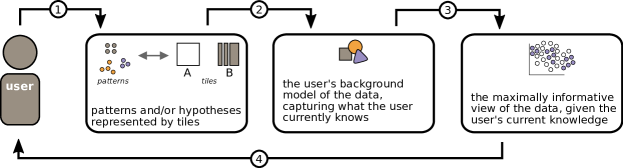
Our framework is sketched in Figure 1. More formally, as in Lijffijt et al. (2014), we denote the original data set by $X$ and the set of all possible data sets by $\Omega$. We further define a set of constraints ${\mathcal{C}}$. A constraint $t\in{\mathcal{C}}$ is simply a subset of all possible data sets which always also includes the original data set, that is, $X\in t\subseteq\Omega$ is satisfied for all $t\in{\mathcal{C}}$. Any set of constraints ${\cal{T}}\subseteq{\mathcal{C}}$ can be used to define a subset of data sets $\Omega_{\cal{T}}\subseteq\Omega$ that satisfy all of the constraints in ${\cal{T}}$ by $\Omega_{\cal{T}}=\cap_{t\in{\cal{T}}}{t}$, with $\Omega_{\emptyset}$ defined as $\Omega_{\emptyset}=\Omega$.

We assume that the user observes a set of relations such as correlations, cluster structures etc. from the data, as later defined by Definition 3. A constraint—or a set of constraints—can either preserve or break a relation. If the user observes that some relations are preserved in the data the user can infer that the data obeys the constraints that preserve these relations.

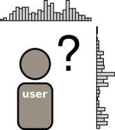
In this paper we assume that the user’s knowledge can be parametrised by a set of constraints ${\cal T}_{u}$ and by a uniform distribution over data sets in $\Omega_{{\cal{T}}_{u}}$, with the probability of the data sets in the complement $\Omega\setminus\Omega_{{\cal{T}}_{u}}$ being zero. We call this uniform distribution a background distribution, which describes the probabilities the user gives for different possible data sets. Intuitively, the constraints denote the relations (or patterns) in the data that the user already is aware of. In the user’s mind, any data set that is not contradictory with any of these constraints is equiprobable, while data sets contradicting with any of the constraints have zero probability. In the absence of constraints, that is, when the user knows nothing, the user’s knowledge is described by the background distribution corresponding to the situation that the user considers all possible data sets equally likely, as shown in Figure 2. Our objective is that the system would not show the user relations or patterns that the user is already aware of, as parametrised by constraints in ${\cal T}_{u}$.

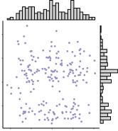
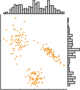
Now, out of all possible views of the data (such as scatter plots over different coordinate axes) the most informative view should be the one that—according to some measure—shows the maximal difference between the data set $X$ and a data set sampled from the background distribution as in Figure 3. When looking at this view, the user may learn more about the relations in the data and can add the gained knowledge as new constraints in ${\cal{T}}_{u}$, after which a new maximally informative view can be produced. This iterative process continues until the user has learned all he or she wants to know about the data; this is the approach taken, for example, in Puolamäki et al. (2016) and Puolamäki, Oikarinen, Kang, Lijffijt, and Bie (2018). As already mentioned, the drawback of the approach is that each new view is by definition also maximally surprising to the user and there is no way to guide the exploration towards the user’s interests.

In this paper we complement this framework by using the constraints to parametrise, in addition to the user’s knowledge, what the user wants to know about the data. We do this by defining a new set of constraints, denoted by ${\cal{T}}_{H}\subseteq{\cal{C}}$ which defines the relations that are of the interest to the user. We further define a set of constraints ${\cal{T}}_{H^{\prime}}\subseteq{\cal{C}}$ which defines the relations that are of no interest to the user. Instead of comparing the data and the background distribution, as earlier, we find a view that shows the maximal difference between samples from the uniform distributions from $\Omega_{{\cal{T}}_{u}\cup{\cal{T}}_{H^{\prime}}}$ and $\Omega_{{\cal{T}}_{u}\cup{\cal{T}}_{H^{\prime}}\cup{\cal{T}}_{H}}$, respectively. Notice that if we are interested in all constraints, i.e., ${\cal{T}}_{H}={\cal{C}}$ and ${\cal{T}}_{H^{\prime}}=\emptyset$, this new formulation reduces to the earlier approach of Puolamäki et al. (2016) and Puolamäki, Oikarinen, Kang, Lijffijt, and Bie (2018), at least if all of the constraints together allow only the original data set, or $\Omega_{{\cal{C}}}=\{X\}$.

Informative view		Uninformative view

Figure 3: Two data samples (shown in orange and purple) in two projections. A view is informative if the data samples differ, which means that the user can learn something new about the data. In the left view the data samples differ with respect to the attributes $C$ and $D$ and the view is informative. In contrast, in the right view the data samples are essentially the same and the user learns nothing new about the relation between attributes $A$ and $B$, and consequently the view is uninformative.

The advantage of the new formulation is that by expressing the user’s knowledge and the user’s objectives using the same parametrisation we can in an elegant way formalise the data exploration process as finding views that show differences between two distributions, or between samples from two distributions.

The above discussion is generic for all classes of data sets and constraints. However, in the remainder of the paper we assume that the data set $X$ is a data table with rows corresponding to data items and columns to attributes, and the set $\Omega$ consists of all data sets that can be obtained by randomly permuting the columns of $X$. The constraints in ${\cal{C}}$ are parametrised by tiles containing subsets of rows and columns, respectively. Samples from the constrained distribution can then be obtained efficiently by permutations, as described later in Section 2, which also gives the exact definitions for the concepts mentioned above. The views considered in this paper are scatterplots of the data obtained by linear projections that show the maximal differences of the distributions described above.

Contributions

In summary, our contributions are:

1. a computationally efficient formulation and implementation of the user’s background knowledge of the data and objectives (which we here call hypotheses) using constrained randomisation,

2. a dimensionality reduction method for finding the view most informative to the user, and

3. an experimental evaluation that supports that our approach is fast, robust, and produces easily understandable results.

Outline

The rest of this paper is organised as follows. Our framework is formalised in Section 2, where we describe how to model the user’s background knowledge of the data, how data exploration objectives are formulated and updated, and how maximally informative views are determined. In Section 3 we empirically evaluate our framework, by considering both computational efficiency and robustness against noise, as well as provide use cases of user-guided exploration. We conclude the paper with a discussion in Section 4.

2 Methods

Let $X$ be an $n\times m$ data matrix (data set). Here $X(i,j)$ denotes the $i$th element in column $j$. Each column $X(\cdot,j),\ j\in[m]$, is an attribute in the data set, where we use the shorthand $[m]=\{1,\ldots,m\}$. Let $D$ be a finite set of domains (for example, continuous or categorical) and let $D(j)$ denote the domain of $X(\cdot,j)$. Also let $X(i,j)\in D(j)$ for all $i\in[n]$ and $j\in[m]$, that is, all elements in a column belong to the same domain but different columns can have different domains. The derivations in Sections 2.1 and 2.2 are generic with respect to domains, but in Section 2.3 we consider only real numbers, that is, $D(j)\subseteq\mathbb{R}$ for all $j\in[m]$.

2.1 Permutations and Tile Constraints

We proceed to introduce the permutation-based sampling method and tile constraints which are used to constrain the sampled distributions as well as to express the user’s background knowledge and objectives (hypotheses). The distributions are constructed so that in the absence of constraints (tiles) the marginal distributions of the attributes are preserved.

We define a permutation of the data matrix $X$ as follows.

Definition 1 (Permutation)

Let ${\mathcal{P}}_{n}$ denote the set of permutation functions of length $n$ such that $\pi:[n]\to[n]$ is a bijection for all $\pi\in{\mathcal{P}}_{n}$, and denote by $\Pi=\left(\pi_{1},\ldots,\pi_{m}\right)\in{\mathcal{P}}^{m}_{n}$ the vector of column-specific permutations. A permutation $\Pi(X)=\widehat{X}$ of a $n\times m$ data matrix $X$ is then given as $\widehat{X}(i,j)=X(\pi_{j}(i),j)$.

When permutation functions are sampled uniformly at random, we obtain a uniform sample from the distribution of data sets where each of the attributes has the same marginal distribution as the original data. Hence, given a data set $X$, the set of possible data sets is $\Omega=\{\Pi(X)\mid\Pi\in{\mathcal{P}}^{m}_{n}\}$.

Unconstrained permutation
All attributes $A,\ldots,D$ are permuted independently. This breaks all relations between the attributes, but the marginals are preserved.

Constrained permutation
The permutation is constrained with a tile, that is, attributes in the tile are permuted together. The marginals are also preserved.

Figure 4: An unconstrained permutation (top) and a permutation constrained with a tile (bottom, tile shown with a solid border). The data has four attributes ($A,B,C$, and $D$) and there are five data items (rows) in the data set.

A tile is a tuple $t=(R,C)$, where $R\subseteq[n]$ and $C\subseteq[m]$. The tiles considered here are combinatorial (in contrast to geometric), meaning that rows and columns in the tile do not need to be consecutive. In the unconstrained case, there are $(n!)^{m}$ allowed vectors of permutations. We parametrise distributions using tile constraints preserving the relations in a data matrix $X$ for subsets of rows and columns. The tiles constrain the set of allowed permutations as follows.

Definition 2 (Tile constraint)

Given a tile $t=(R,C)$ where $R\subseteq[n]$ and $C\subseteq[m]$, a vector of permutations $\Pi=\left(\pi_{1},\ldots,\pi_{m}\right)\in{\mathcal{P}}^{m}_{n}$ is allowed by $t$ iff the following condition is true for all $i\in[n]$, $j\in[m]$, and $j^{\prime}\in[m]$:

$$i\in R\textrm{ and }j,j^{\prime}\in C\\ \implies\pi_{j}(i)\in R\textrm{ and }\pi_{j}(i)=\pi_{j^{\prime}}(i).$$

Given a set of tiles $T$, a vector of permutations $\Pi$ is allowed iff $\Pi$ is allowed by all $t\in T$. For an empty set of tiles $T=\emptyset$, all permutations in ${\mathcal{P}}^{m}_{n}$ are allowed.

A tile defines a subset of rows and columns, and the rows in this subset are permuted by the same permutation function in each column in the tile. In other words, the relations between the columns inside the tile are preserved. Thus, given a data set $X$ and a set of tiles $T$, the subset of data sets in $\Omega$ that satisfy all of the tile constraints in $T$ is given by

$$\Omega_{T}=\{\Pi(X)\mid\Pi\in{\mathcal{P}}^{m}_{n}\mbox{ and }\Pi\mbox{ is allowed by }T\}.$$

Notice that the identity permutation is always an allowed permutation. Figure 4 shows an example of both unconstrained permutation and permutation constrained with a tile.

We proceed to define formally what we mean by relations in this paper.

Definition 3 (Relation)

A relation is a real-valued function $f$ over $n\times m$ data matrices $X$. Given a set of tiles $T$, we say that that $T$ preserves the relation $f$, if $f(X)=f(\Pi(X))$ is satisfied for all permutations $\Pi$ allowed by $T$. Otherwise, we say that $T$ breaks the relation $f$.

Thus, we use the term relation to denote any structure in the data which can be controlled (that is, essentially broken if need be) in the permutation scheme parametrised by the tile constraints. In practise, some tolerance could be included in the above definition for the condition $f(X)=f(\Pi(X))$ instead of exact equivalence. Examples of relations conforming to the above definition include correlations between attributes, and cluster structures. For example, for a real valued data matrix a relation could be defined as a covariance between columns $a$ and $b$, i.e., $f(X)=\sum\nolimits_{i=1}^{n}{X(i,a)X(i,b)}/n$. A set of tiles containing a tile $t=([n],\{a,b\})$ preserves this relation. On the other hand, a set of tiles allowing some of the rows in columns $a$ and $b$ to be permuted independently breaks the relation $f$. Another example of a possible relation are the scagnostics for a scatterplot visualisation (Wilkinson et al., 2005).

We make an implicit assumption that if the user observes in the data that certain (visual) relations are preserved, then the user can conclude that the data also obeys constraints that preserve those same relations. The user can then add these constraints to the background distribution. Note that the relations $f$ correspond to visual patterns (correlations, cluster structures, outliers etc.) which the user possibly observes. The relations $f$ are not evaluated by the computer, but they are part of the user’s cognitive processing of the visualisations. Therefore, in practical applications, there is usually no need—nor would it be possible—to define all of the relations $f$ explicitly. For our purposes it suffices that the user can to a reasonable accuracy match the observed visual relations in the data to the corresponding constraints.

We use tile constraints to describe the user’s knowledge concerning relations in the data. As the user views the data he or she can observe relations and represent these as tile constraints. For example, the user can mark an observed cluster structure with a tile involving the data points in the cluster and the relevant attributes. We denote the set of user-defined tiles by ${\mathcal{T}}_{u}$. Then, a uniform distribution from $\Omega_{{\cal T}_{u}}=\{\Pi(X)\mid\Pi\in{\mathcal{P}}^{m}_{n}\mbox{ and }\Pi\mbox{ is allowed by }{\cal T}_{u}\}$ is the background distribution, which describes the probabilities the user gives for different possible data sets.

We can now formulate our sampling problem as follows.

Problem 4 (Sampling problem)

Given a set of tiles $T$, draw samples uniformly at random from vectors of permutations $\Pi\in{\mathcal{P}}^{m}_{n}$ allowed by $T$.

The sampling problem is trivial when the tiles are non-overlapping, since permutations can be done independently within each non-overlapping tile. However, in the case of overlapping tiles, multiple constraints can affect the permutation of the same subset of rows and columns and this issue must be resolved. To this end, we need to define the equivalence of two sets of tiles, which means that the same constraints are enforced on the permutations.

Definition 5 (Equivalence of sets of tiles)

Let $T$ and $T^{\prime}$ be two sets of tiles. $T$ is equivalent to $T^{\prime}$, if for all vectors of permutations $\Pi\subseteq\mathcal{P}^{m}_{n}$ it holds:

$$\Pi\mbox{ is allowed by }T\mbox{ iff }\Pi\mbox{ is allowed by }T^{\prime}.$$

Figure 5: Merging the two overlapping purple (solid border) and orange (dashed border) tiles leads to three non-overlapping tiles. Data as in Figure 4.

We use the term tiling for a set of tiles $\mathcal{T}$ where no tiles overlap. Next, we show that there always exists a tiling equivalent to a set of tiles.

Theorem 6

Given a set of (possibly overlapping) tiles $T$, there exists a tiling $\mathcal{T}$ that is equivalent to $T$.

Proof  Let $t_{1}=(R_{1},C_{1})$ and $t_{2}=(R_{2},C_{2})$ be two overlapping tiles. Each tile describes a set of constraints on the allowed permutations of the rows in their respective column sets $C_{1}$ and $C_{2}$. A tiling $\{t^{\prime}_{1},t^{\prime}_{2},t^{\prime}_{3}\}$ equivalent to $\{t_{1},t_{2}\}$ is given by:

$$\begin{array}[]{rcl}t^{\prime}_{1}&=&(R_{1}\setminus R_{2},C_{1}),\\ t^{\prime}_{2}&=&(R_{1}\cap R_{2},C_{1}\cup C_{2}),\\ t^{\prime}_{3}&=&(R_{2}\setminus R_{1},C_{2}).\end{array}$$

Tiles $t^{\prime}_{1}$ and $t^{\prime}_{3}$ represent the non-overlapping parts of $t_{1}$ and $t_{2}$ and the permutation constraints by these parts can be directly met. Tile $t^{\prime}_{2}$ takes into account the combined effect of $t_{1}$ and $t_{2}$ on their intersecting row set, in which case the same permutation constraints must apply to the union of their column sets. It follows that these three tiles are non-overlapping and enforce the combined constraints of tiles $t_{1}$ and $t_{2}$. Hence, a tiling can be constructed by iteratively resolving overlap in a set of tiles until no tiles overlap.  
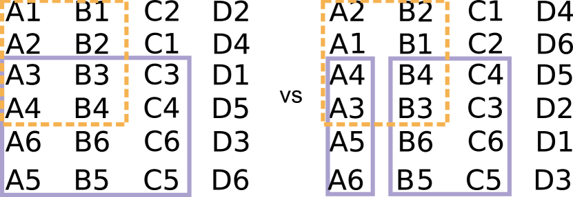
Notice that merging overlapping tiles leads to wider (larger column set) and lower (smaller row set) tiles. An example is shown in Figure 5. The limiting case is a fully-constrained situation where each row is a separate tile and only the identity permutation is allowed. We provide an efficient algorithm with the time complexity $\mathcal{O}{(nm)}$ for merging tiles in Appendix A.

2.2 Formulating Hypotheses

As discussed in the introduction, in order to model what the user wants to know about the data, we define two sets of constraints: ${\cal{T}}_{H}$ (the relations that are of the interest for the user) and ${\cal{T}}_{H^{\prime}}$ (the relations that are of no interest for the user). We then find a view that shows the maximal difference between the uniform distributions from $\Omega_{{\cal{T}}_{u}\cup{\cal{T}}_{H^{\prime}}}$ and $\Omega_{{\cal{T}}_{u}\cup{\cal{T}}_{H^{\prime}}\cup{\cal{T}}_{H}}$, respectively. We now formalise this idea by formulating a pair of hypotheses, concisely represented using the tilings defined in the previous section. This provides a flexible method for the user to specify the relations in which he or she is interested.

Definition 7 (Hypothesis tilings)

Given a subset of rows $R\subseteq[n]$, a subset of columns $C\subseteq[m]$, and a $k$-partition of the columns given by $C_{1},\ldots,C_{k}$, such that $C=\cup_{i=1}^{k}{C_{k}}$ and $C_{i}\cap C_{j}=\emptyset$ if $i\neq j$, a pair of hypothesis tilings is given by $\mathcal{T}_{H_{1}}=\{(R,C)\}$ and $\mathcal{T}_{H_{2}}=\cup_{i=1}^{k}{\{(R,C_{i})\}}$.

The hypothesis tilings define the items $R$ and attributes $C$ of interest, and, through the partition of $C$, the relations between the attributes in which the user is interested. Hypothesis 1 ($\mathcal{T}_{H_{1}}$) corresponds to a uniform distribution from the data sets in which all relations in $(R,C)$ are preserved, and hypothesis 2 ($\mathcal{T}_{H_{2}}$) to a uniform distribution from the data sets in which the relations between attributes in the partitions $C_{1},\ldots,C_{k}$ of $C$ are broken while the relations between attributes inside each $C_{i}$ are preserved. In terms of the constraints, as discussed in Section 1, relations preserved by $\mathcal{T}_{H_{2}}$ correspond to the relations which the user is not interested in (that is, ${\cal{T}}_{H^{\prime}}$ in Section 1), while relations preserved by $\mathcal{T}_{H_{1}}$ but broken by $\mathcal{T}_{H_{2}}$ correspond to relations which user is interested in (that is, ${\cal{T}}_{H}$ in Section 1).

Case 1: Are there relations between any of the attributes?

Case 2: Are there relations between any of the attributes other than those constrained by the tile shown with an orange dashed border?

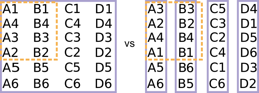
Case 3: Are there relations between the attribute groups $\{A\}$ and $\{B,C\}$ for items $\{3,4,5,6\}$ other than those constrained by the tile with an orange dashed border?

Figure 6: Modelling hypotheses using sets of tiles. Tilings corresponding to hypotheses are shown with solid purple borders: Hypothesis 1 on the left and Hypothesis 2 on the right. The user’s knowledge is represented by the tile with a dashed orange border. The data set has four attributes $A,B,C$ and $D$, and six data items. See Section 2.5 for an interpretation of these operations in terms of the iris flower data.

Now, for example, if the columns are partitioned into two groups $C_{1}$ and $C_{2}$ the user is interested in relations between the attributes in $C_{1}$ and $C_{2}$, but not in relations within $C_{1}$ or $C_{2}$. On the other hand, if the partition is full, that is, $k=|C|$ and $|C_{i}|=1$ for all $i\in[k]$, then the user is interested in all relations between the attributes inside $(R,C)$. The special case of $R=[n]$ and $C=[m]$ indeed reduces to unguided data exploration, where all inter-attribute relations in the data are of interest to the user.

Having defined both the user’s knowledge (background distribution) and the pair of hypotheses formalising the user’s objectives with tile constraints, we can now easily combine these to formalise the uniform distributions from the data sets we want to compare. I.e., we want to compare the uniform distributions from $\Omega_{\mathcal{T}_{u}+\mathcal{T}_{H_{1}}}$ and $\Omega_{\mathcal{T}_{u}+\mathcal{T}_{H_{2}}}$, where ‘$+$’ is used with a slight abuse of notation to denote the operation of merging two tilings (with possible overlaps between their tiles) into an equivalent tiling. Notice here that, by Definition 7, it holds that

$$\Omega_{\mathcal{T}_{u}+\mathcal{T}_{H_{1}}}\subseteq\Omega_{\mathcal{T}_{u}+\mathcal{T}_{H_{2}}},$$

and hence the comparison becomes equivalent to the formulation provided in the introduction. Recall that we can draw samples from these distributions as described in Section 2.1. From now on, we use the term hypothesis pair $\mathcal{H}$ to denote

$$\mathcal{H}=\langle\mathcal{T}_{u}+\mathcal{T}_{H_{1}},\mathcal{T}_{u}+\mathcal{T}_{H_{2}}\rangle,$$

where $\mathcal{T}_{u}$ is the tiling formalising the (current) background distribution, and $\mathcal{T}_{H_{1}}$ and $\mathcal{T}_{H_{2}}$ form a pair of hypothesis tilings as defined in Definition 7. See Figure 6 for examples of different cases in which a pair of hypothesis tilings and the user’s knowledge are used to explore relations between attributes. Here, the first case demonstrates a scenario in which the user is interested in all relations, and hence the set of relations that are of no interest to the user ${\cal{T}}_{H^{\prime}}$ is empty. Furthermore, the user has no prior knowledge, that is, ${\cal{T}}_{u}=\emptyset$. The second case is similar, but here the tile shown with an orange dashed border represents the user’s knowledge ${\cal{T}}_{u}\neq\emptyset$. Finally, the third case shows a scenario in which ${\cal{T}}_{H^{\prime}}\neq\emptyset$. The relations preserved between attributes $B$ and $C$ for items $\{3,4,5,6\}$ are of no interest to the user, while the relations between the attribute groups $\{A\}$ and $\{B,C\}$ are.

2.3 Finding Views

We are now ready to formulate our second main problem, that is, given the uniform distributions from the two data sets characterised by the hypothesis pair $\mathcal{H}$, how can we find an informative view of the data maximally contrasting these? The answer to this question depends both on the type of data and the selected visualisation. For example, visualisations or measures of difference are different for categorical and real-valued data. The real-valued data discussed in this paper allows us to use projections (such as principal components) that mix attributes.

Problem 8 (Comparing hypotheses)

Given the two uniform distributions characterised by the hypothesis pair $\mathcal{H}=\langle\mathcal{T}_{u}+\mathcal{T}_{H_{1}},\mathcal{T}_{u}+\mathcal{T}_{H_{2}}\rangle$, find the projection in which the distributions differ the most.

To solve this problem, we devise a linear projection pursuit method which finds the direction in which the two distributions differ the most in terms of variance. In principle some other difference measure could be used instead. However, a variance-based measure can be implemented efficiently, which is one essential requirement for interactive use. Furthermore, using variance leads to the convenient property that our projection pursuit method reduces to standard principal component analysis (PCA) when the user has no background knowledge and when the hypotheses are most general, as shown in Theorem 11 below.

Thus, we formalise the optimisation criterion in Problem 8 by defining a measure using variance. Specifically, we choose the following form for our gain function:

$$G(v,\mathcal{H})=\frac{v^{T}\Sigma_{1}v}{v^{T}\Sigma_{2}v},$$ (1)

where $v$ is a vector in $\mathbb{R}^{m}$ and $\Sigma_{1}$ and $\Sigma_{2}$ are the covariance matrices of the uniform distributions from the data sets in $\Omega_{\mathcal{T}_{u}+\mathcal{T}_{H_{1}}}$ and $\Omega_{\mathcal{T}_{u}+\mathcal{T}_{H_{2}}}$, respectively. Then, the direction in which the distributions differ most in terms of the variance, that is, the solution to Problem 8, is given by

$$v_{\mathcal{H}}=\operatorname*{arg\,max}_{v\in\mathbb{R}^{m}}G(v,\mathcal{H}).$$ (2)

In order to solve Problem 8, we first show that the covariance matrix $\Sigma$ for a distribution defined using the permutation-based scheme with tile constraints can be computed analytically.

Theorem 9

Given $j,j^{\prime}\in[m]$, the covariance of attributes $\mathrm{cov}(j,j^{\prime})$ from the uniform distribution of data sets $\Omega_{\mathcal{T}}$ defined by a tiling $\mathcal{T}$ is given by $\mathrm{cov}(j,j^{\prime})=\sum\nolimits_{i=1}^{n}{a_{j}(i)a_{j^{\prime}}(i)}/n$, where

$$a_{l}(i)=\left\{\begin{array}[]{ll}Y(i,l),&i\in R_{j,j^{\prime}}\\ \sum\nolimits_{k\in R(i,l)}{Y(k,l)}/|R(i,l)|,&i\notin R_{j,j^{\prime}}\end{array}\right.$$

and $l\in\{j,j^{\prime}\}$. Here, $R_{j,j^{\prime}}=\{i\in[n]\mid\exists(R,C)\in\mathcal{T}\textrm{ where }i\in R\textrm{ and }j,j^{\prime}\in C\}$ denotes the set of rows permuted together, $Y(i,l)=X(i,l)-\sum\nolimits_{i=1}^{n}{X(i,l)}/n$ denotes the centred data matrix, and $R(i,l)\subseteq[n]$ denotes a set satisfying $\exists C\subseteq[m]$ where $(R(i,l),C)\in\mathcal{T}$, $i\in R(i,l)$ and $l\in C$, that is, the rows in a tile that the data point $X(i,l)$ belongs to.

Proof  The covariance is defined by

$$\mathrm{cov}(j,j^{\prime})=E\left[\sum\nolimits_{i=1}^{n}{Y(\pi_{j}(i),j)Y(\pi_{j^{\prime}}(i),j^{\prime})}/n\right],$$

where the expectation $E[\cdot]$ is defined over the permutations $\pi_{j}\in{\cal P}^{n}$ and $\pi_{j^{\prime}}\in{\cal P}^{n}$ of columns $j$ and $j^{\prime}$ allowed by the tiling $\mathcal{T}$, respectively. The part of the sum for rows permuted together $R_{j,j^{\prime}}$ reads

$$\sum\nolimits_{i\in R_{j,j^{\prime}}}{E\left[Y(\pi_{j}(i),j)Y(\pi_{j^{\prime}}(i),j^{\prime})\right]}/n=\sum\nolimits_{i\in R_{j,j^{\prime}}}{Y(i,j)Y(i,j^{\prime})}/n,$$

where we have used $\pi_{j}(i)=\pi_{j^{\prime}}(i)$ and reordered the sum for $i\in R_{j,j^{\prime}}$. The remainder of the sum reads

$$\sum\nolimits_{i\in R_{j,j^{\prime}}^{c}}{E\left[Y(\pi_{j}(i),j)Y(\pi_{j^{\prime}}(i),j^{\prime})\right]}/n=\sum\nolimits_{i\in R_{j,j^{\prime}}^{c}}{E\left[Y(\pi_{j}(i),j)\right]E\left[Y(\pi_{j^{\prime}}(i),j^{\prime})\right]}/n,$$

where $R_{j,j^{\prime}}^{c}=[n]\setminus R_{j,j^{\prime}}$ and the expectations have been taken independently, because the rows in $R_{j,j}^{c}$ are permuted independently at random. The result then follows from the observation that $E\left[Y(\pi_{l}(i),l)\right]=a_{l}(i)$ for any $i\in R_{j,j^{\prime}}^{c}$.  

The direction in which the ratio of the variances is the largest can now be found by applying a whitening operation (Kessy et al., 2018) on $\Sigma_{2}$. The idea of whitening is to find a whitening matrix $W$ such that $W^{T}\Sigma_{2}W=I$. Using this transformation in Equation (1) makes the denominator constant, and we hence obtain the solution to the optimisation in Equation (2) by finding the principal components of $\Sigma_{1}$ transformed using $W$.

Theorem 10

The solution to the optimisation problem of Equation (2) is given by $v_{\mathcal{H}}=Ww$, where $w$ is the first principal component of $W^{T}\Sigma_{1}W$ and $W\in{\mathbb{R}}^{m\times m}$ is a whitening matrix such that $W^{T}\Sigma_{2}W=I$.

Proof Using $v=Ww$ the gain in Equation (1) can be rewritten as

$$G(Ww,\mathcal{H}) =\frac{w^{T}W^{T}\Sigma_{1}Ww}{w^{T}W^{T}\Sigma_{2}Ww}=\frac{w^{T}W^{T}\Sigma_{1}Ww}{w^{T}w}.$$ (3)

Equation (3) is maximised when $w$ is the maximal variance direction of $W^{T}\Sigma_{1}W$, from which it follows that the solution to the optimisation problem of Equation (2) is given by $v_{\mathcal{H}}=Ww$, where $w$ is the first principal component of $W^{T}\Sigma_{1}W$.  

Note

In visualisations (that is, when making two-dimensional scatterplots), we project the data onto the first two principal components, instead of considering only the first component as above.

Finally, we are ready to show that at the limit of no background knowledge and with the most general hypotheses, our method reduces to PCA of the correlation matrix.

Theorem 11

In the special case of the first step in unguided data exploration, that is, comparing distributions from a hypotheses pair specified by $\mathcal{H}=\langle\emptyset+\mathcal{T}_{H_{1}},\emptyset+\mathcal{T}_{H_{2}}\rangle$, where $\mathcal{T}_{H_{1}}=\{([n],[m])\}$ and $\mathcal{T}_{H_{2}}=\cup_{j=1}^{m}\{([n],\{j\})\}$, the solution to Equation (2) is given by the first principal component of the correlation matrix of the data, when the data attributes have been scaled to unit variance.

Proof  The proof follows from the observations that for $\mathcal{T}_{H_{2}}$ the covariance matrix $\Sigma_{2}$ is a diagonal matrix (here a unit matrix), resulting in the whitening matrix $W=I$. For this pair of hypothesis, $\Sigma_{1}$ denotes the covariance matrix of the original data. The result then follows from Theorem 10.  

Once we have defined the most informative projection, which displays the directions in which the distributions parametrised by the hypothesis pair $\mathcal{H}$ differ the most, we can show the original data in this projection. This allows the user to observe different patterns, for example, a clustered set of points, a linear relationship, or a set of outlier points. We note that it would also be possible to show and compare samples from the two distributions characterised by the hypothesis pair $\mathcal{H}$ in the most informative view. In Henelius et al. (2018) we presented a proof-of-concept tool using which the user can, in fact, toggle between showing the data and samples from the two distributions representing the hypotheses. This can potentially shed some further light into why this particular view is interesting, but as we are mostly interested in the relations present in the actual data, we have chosen for simplicity to consider only the data in the most informative projection in this work.

2.4 Selecting Attributes for a Tile Constraint

After observing a pattern, the user can define a tile $(R,C)$ to be added to $\mathcal{T}_{u}$. The set of data points $R$ included in the pattern can be easily selected from the projection shown. For selecting the attributes characterising the pattern, we use a procedure where for each attribute the ratio between the standard deviation of the attribute for the selection and the standard deviation of all data points is computed. If this ratio is below a threshold value $\tau$ (for example, $\tau=0.5$), then the attribute is included in the set of attributes $C$ characterising the pattern. The intuition here is that we are looking for attributes in which the selection of points are more similar to each other than is expected based on the whole data. Thus, the set of attributes for which the user’s knowledge of dependencies is included, is affected by the choice of $\tau$. A smaller value of $\tau$ will only include attributes for which the selection of points is very similar, whereas a larger value of $\tau$ will include a larger set of attributes to the tile constraint. A parallel coordinates plot ordered according to the ratio of standard deviations can be useful in deciding a suitable value for $\tau$, see Section 3.3 for examples in which we use parallel coordinate plots.

(a)	(b)	(c)

Figure 7: (a) Scatterplot matrix of the toy data set. (b) Fully randomised data (orange circles) modelling the user’s knowledge and data (purple squares) where only the relation between attributes $C$ and $D$ has been preserved modelling what the user could learn of the relations between attributes $C$ and $D$. (c) As in (b), but additionally the relation between attributes $A$ and $C$, as well as between attributes $B$ and $D$, has been preserved, modelling the user’s knowledge of the relations between $A$ and $C$ as well as $B$ and $D$, respectively.

2.5 Example: Iris Data

The iris flower dataset is a well-known machine learning dataset. It consists of four measurements on 150 iris flowers from three species (Fisher, 1936). In this section we discuss, for illustration, what the operations shown in Figure 6 could mean in terms of the iris data.

Assume that the four attributes $A$–$D$ in Figure 6 are the four measurements: petal length ($A$), petal width ($B$), sepal length ($C$), and sepal width ($D$). Further assume that rows 1–2 correspond to the species setosa, rows 3–4 to the species versicolor, and rows 5–6 to the species virginica, and that the attributes have been scaled to zero mean and unit variance.

Case 1 of Figure 6 corresponds to the PCA projection of the iris data, as stated by Theorem 11. The first PCA component, given by Equation (2), is $v_{\mathcal{H}}=-0.58\times A-0.56\times B-0.52\times C+0.26\times D$, implying that the overall correlations of the data are best described by (roughly) the average petal length ($A$), petal width ($B$), and sepal length ($C$).

In Case 2 we assume that the user is aware of the high correlation of petal length ($A$) and petal width ($B$) for the species setosa and versicolor, which is expressed by the tile with the orange dashed border in Figure 6. With this constraint, the direction provided by Equation (2) is given by $v_{\mathcal{H}}=-0.73\times A+0.11\times B-0.58\times C+0.34\times D$. The weight of the petal width is reduced—the user already knows about its correlation with petal length—and the weight of the other measurements is increased.

In Case 3 the user is interested only in the species versicolor and virginica and the correlation between petal length ($A$) and petal width and sepal length ($B$–$C$). In this case the most informative direction given by Equation (2) is $v_{\mathcal{H}}=0.50\times A-0.77\times B+0.39\times C+0\times D$. Sepal width ($D$) is no longer informative, because it is not connected to the hypothesis pair $\mathcal{H}$, and it appears in the projection with a zero weight.

Summarising, the projection therefore tends to emphasize more the directions that are most informative to the user, of which we show more examples in Section 3.

2.6 Example: Analysing Partitions of Data Items

Partitioning of data items or subsets of data items can be found, e.g., by clustering algorithms, by using known categorical attributes, or by visual inspection, as we will later demonstrate in Sections 3.3 and 3.4. Our approach is suitable for probing such subsets of data items and finding relations in data that are not explained by the given data subset.

At the simplest, if we are given a subset of data items of interest, we can use the hypothesis tiling of Definition 7 to probe the subset of rows $R$ of interest. Another straightforward to include a subset of data items $R$ into the user’s background information would be to add a tile $(R,[m])$ to $\mathcal{T}_{u}$, after which the system would ignore the data items in $R$. More nuanced examples of adding subsets of data points into background information are given in Section 3.

2.7 Example: Subsetting Loses Information

We conclude this section with a simple example illustrating how subsetting the data in order to focus on a specific objective can lead to loss of information. With this example we wish to highlight two aspects: (i) how the user’s background knowledge and objectives affect the views that are most informative, and (ii) how it can be advantageous to investigate relations in the data as a whole instead of using a subset of the data for the analysis.

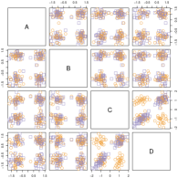
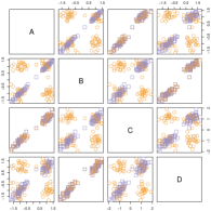
We construct a toy data set with four attributes $A$, $B$, $C$, and $D$ as follows. We first generate two strongly correlated attributes $A$ and $B$, after which we generate attribute $C$ by adding noise to $A$, and attribute $D$ by adding noise to $B$. This data set, visualised in Figure 7(a), is very simple and here it is possible to investigate all pairwise relations in the data in one view. This is in general not possible in any real analysis scenarios. Furthermore, we assume that the user is interested in the relation between attributes $C$ and $D$. Our goal is then to find a maximally informative 1-dimensional projection of the data that takes both this objective and the user’s background knowledge into account.

First, let us assume that the user only knows the marginal distribution of each attribute but is unaware of the relations between the attributes. Using the approach in this paper we formulate this by means of the hypothesis pair $\mathcal{H}_{0}=\langle\mathcal{T}_{u_{0}}+\mathcal{T}_{H_{1}},\mathcal{T}_{u_{0}}+\mathcal{T}_{H_{2}}\rangle$, where $\mathcal{T}_{u_{0}}=\emptyset$, $\mathcal{T}_{H_{1}}=\{(R,\{C,D\})\}$, $\mathcal{T}_{H_{2}}=\{(R,\{C\}),(R,\{D\})\}$, and $R=[n]$ (all rows in the data). A sample from $\Omega_{\mathcal{T}_{u_{0}}+\mathcal{T}_{H_{1}}}$ is shown in Figure 7(b) using purple squares, and a sample from $\Omega_{\mathcal{T}_{u_{0}}+\mathcal{T}_{H_{2}}}$ is shown using orange circles. The orange distribution hence models what the user currently knows and the purple what the user could optimally learn about the relation between $C$ and $D$ from the data. The orange and purple distributions differ the most in the plot $CD$, as expected, and indeed the maximally informative 1-dimensional projection satisfying Equation (2), is given by $v=0.7C+0.7D$.

Secondly, assume that, unlike above, the user is already aware of the relationship between the attribute pairs $A$ and $C$ as well as $B$ and $D$, but does not know that attributes $A$ and $B$ are almost identical. We proceed as above with the difference that we now add the user’s knowledge as a constraint to both the distributions. This is achieved by updating the hypothesis pair to $\mathcal{H}_{1}=\langle\mathcal{T}_{u_{1}}+\mathcal{T}_{H_{1}},\mathcal{T}_{u_{1}}+\mathcal{T}_{H_{2}}\rangle$, where $\mathcal{T}_{u_{1}}=\{(R,\{A,C\}),(R,\{B,D\})\}$ captures the user’s knowledge.

Samples from the uniform distributions on the data sets conforming to this hypothesis pair are shown in Figure 7(c). Again, the orange distribution models the user’s knowledge (that is, $\Omega_{\mathcal{T}_{u_{1}}+\mathcal{T}_{H_{2}}}$) and the purple what the user could learn from the relation between $C$ and $D$ from the data, given that the user already knows about the relationships of the attribute pairs $A$ and $C$ as well as $B$ and $D$ (that is, $\Omega_{\mathcal{T}_{u_{1}}+\mathcal{T}_{H_{1}}}$). The orange and purple distributions differ the most in the plot $AB$ and therefore the user would gain most information if shown this view. Indeed, the most informative 1-dimensional projection satisfying Equation (2) is $v=-0.7A-0.7B$. In other words, the knowledge of the relation of $A$ and $B$ gives maximal information about the relation of $C$ and $D$. This makes sense, because the variables $C$ and $D$ are really connected via $A$ and $B$ through their generative process.

This example hence shows how the background knowledge affects the views. Also, if we had chosen a subset of the data containing, for example, just attributes $C$ and $D$ we would not have observed the connection of $C$ and $D$ through $A$ and $B$, even if we knew the relation between $A$ and $C$ as well as $B$ and $D$. Thus, we have demonstrated with this simple example that using hypothesis tilings as above allows us to explore the entire data set at once while still focusing on particular relations of interest.

3 Experiments

In this section we first consider the stability and scalability of the framework presented in this paper. After this, we present examples of how the proposed method is used to explore relations in a data set and to focus on investigating a hypothesis concerning relations in a subset of the data. An open source library implementing the proposed framework, including the code for the experiments presented in this paper, is available from https://github.com/edahelsinki/corand/.

All the experiments were run on a MacBook Pro laptop with a 3.1 GHz Intel Core i5 processor using R version 3.5.2 (R Core Team, 2018).

3.1 Data Sets

We use synthetic data in the scalability experiment. We also use two real-world data sets to showcase the applicability of our framework in human-guided data exploration.

The german socioeconomic data set (Boley et al., 2013; Kang et al., 2016a) contains records from 412 German administrative districts. Each district is represented by 46 attributes describing socioeconomic and political aspects in addition to attributes such as the type of the district (rural/urban), area name/code, state, region (East/West/North/South) and the geographic coordinates of each district center. The socioecologic attributes include, for example, population density, age and education structure, economic indicators (for example, GDP growth, unemployment, income), and the proportion of the workforce in different sectors. The political attributes include election results of the five major political parties (CDU/CSU, SPD, FDP, Green, and Left) in the German federal elections in 2005 and 2009, as well as the voter turnout. For our experiments we exclude the election results from 2005 (which are highly correlated with the 2009 election results), all non-numeric variables, and the area code and coordinates of the districts, resulting in 32 real-valued attributes (although we use the full data set when interpreting the results). Finally, we scale the real-valued variables to zero mean and unit variance.

The accident data set is a random sample of 3000 accidents from a large data set containing all occupational accidents in Finnish enterprises during the period 2003–2014 reported to the Finnish Workers’ Compensation Center. In the original data set, the accidents are described by 37 variables, the majority of which are categorical, including details about the victim (occupation, age, sex, nationality) and the accident (geographical location, cause, type, working process). We use one-hot encoding to transform the categorical variables into real-valued variables, creating a column for every label of every variable in which the presence (absence) of a label is indicated by 1 (0, respectively). To restrict the dimensionality of the resulting encoding, we drop variables with a very high number of labels; for example, the variable for the municipality in which the accident happened has more than 300 labels and would result in equally many columns in the data. Variables with many labels are implicitly given more weight in the one-hot encoding as well. For instance, the attribute sukup (gender) has 2 labels, while the attribute ruumis (injured body part) has 68 labels. In the transformed data there are 2 columns for sukup and 68 columns for ruumis, making the latter more strongly represented in the data. This could impact further analysis, and to overcome this effect, we scaled the binary data in groups, that is, all columns that originate from the same variable are scaled to have a total variance of 1. The resulting data set contains 3000 rows and 220 attributes.

$\bm{\sigma}$	$\bm{\Delta n=0}$	$\bm{\Delta n=100}$	$\bm{\Delta n=200}$
$0$	$0.000$	$0.008$	$0.021$
$1$	$0.049$	$0.058$	$0.096$
$2$	$0.111$	$0.144$	$0.170$
$5$	$0.280$	$0.230$	$0.293$
$10$	$0.358$	$0.302$	$0.308$

Table 1: The mean relative error as a function of perturbance of the data. Here $\sigma$ is the variance of the noise added and $\Delta n$ denotes the number of rows randomly removed. The relative error is the difference in gain of Equation (1) between the optimal solution $v_{\mathcal{H}}$ and the solution $v_{\mathcal{H}}^{*}$ found on perturbed data divided by the gain in the optimal solution.

$\bm{n}$	$\bm{m}$	$\bm{t_{\mathrm{model}}}$ (s)	$\bm{t_{\mathrm{view}}}$ (s)
$500$	$10$	$0.02$	$0.01$
$1000$	$10$	$0.04$	$0.01$
$5000$	$10$	$0.22$	$0.04$
$10000$	$10$	$0.53$	$0.10$
$500$	$50$	$0.06$	$0.14$
$1000$	$50$	$0.10$	$0.20$
$5000$	$50$	$0.41$	$0.81$
$10000$	$50$	$2.01$	$1.65$
$500$	$100$	$0.09$	$0.48$
$1000$	$100$	$0.14$	$0.75$
$5000$	$100$	$0.92$	$3.32$
$10000$	$100$	$3.40$	$6.68$
$500$	$150$	$0.13$	$1.02$
$1000$	$150$	$0.28$	$1.65$
$5000$	$150$	$1.58$	$7.26$
$10000$	$150$	$2.22$	$15.20$
$500$	$200$	$0.25$	$1.74$
$1000$	$200$	$0.40$	$3.05$
$5000$	$200$	$0.84$	$13.08$
$10000$	$200$	$6.67$	$26.37$

Table 2: Median wall clock running time for random data with varying number of rows ($n$) and columns ($m$) for a data set consisting of Gaussian random numbers. We give the time to add three random tiles plus hypothesis tiles ($t_{\mathrm{model}}$) and the time to find the most informative view ($t_{\mathrm{view}}$), that is, to solve Equation (2).

3.2 Stability and Scalability

We first study the sensitivity of the results with respect to noise or missing data rows. In this experiment we use the 32 real-valued variables from the german data together with three (non-trivial) factors, namely Type (2 values), State (16 values), and Region (4 values) to create synthetic data sets. A synthetic data set, parametrised by the noise term $\sigma$ and an integer $\Delta n$ is constructed as follows. First, we randomly remove $\Delta n$ rows from the data, after which Gaussian noise with variance $\sigma^{2}$ is added to the remaining variables, and finally all variables are rescaled to zero mean and unit variance. We create a random tile by randomly picking a factor that defines the rows in a tile and then randomly sample 2 to 32 attributes as the columns. The background knowledge $\mathcal{T}_{u}$ consists of three such random tiles. The hypothesis tiles are constructed using one such random tile $(R,C)$ as a basis: $\mathcal{T}_{H_{1}}=\{(R,C)\}$ and $\mathcal{T}_{H_{2}}=\cup_{j\in C}{\{(R,\{j\})\}}$.

The results are shown in Table 1. We notice that the method is relatively insensitive with respect to the gain in terms of noise and removal of rows. Even removing about half of the rows ($\Delta n=200$) does not change the results meaningfully. Only a very high degree of noise, corresponding to $\sigma\geq 5$ (that is, circa 5–10% signal-to-noise ratio) substantially degrades the results.

Table 2 shows the running time of the algorithm as a function of the size of the data for Gaussian random data with a similar tiling setup as used for the german data. We make two observations. First, the tile operations scale linearly with the size of the data $nm$ and they are relatively fast. Most of the time is spent on finding the views, that is, solving Equation (2). Even our unoptimised pure R implementation runs in seconds for data sets that are visualisable (having thousands of rows and hundreds of attributes); any larger data set should in any case be downsampled for visualisation purposes.

Figure 8: The most informative view of the german data set with respect to the hypothesis pair $\mathcal{H}_{E,\emptyset}$. Black filled circles show the data points; the selected points (Selection 1) are marked with purple. The $x$ and $y$ axis labels show the five attributes with the largest absolute values in each projection vector.

Figure 9: Parallel coordinates plot of the german data set with Selection 1 of Figure 8 highlighted in purple. Here each of the jigged vertical lines corresponds to one of the data items; the colours are as in Figure 8. Each of the horizontal lines corresponds to a data attribute. The values of the attributes have been shifted and scaled so that the minimum value of each attribute is at the left and the maximum value is at the right. The intersection of a horizontal line and a jigged vertical line (data item) corresponds to the value of the attribute for the particular data item. In the parenthesis we show the ratio between the standard deviation of the attribute for the selection (purple data items) and the standard deviation of the attribute for all data items, i.e., the parameter $\tau$ as defined Section 2.4. The attributes have been ordered by decreasing $\tau$, after which the attributes that are most homogeneous for data items in this particular selection are at the bottom.

3.3 Exploration of the German Data Set

Next, we demonstrate our framework by exploring the german data set under different objectives.

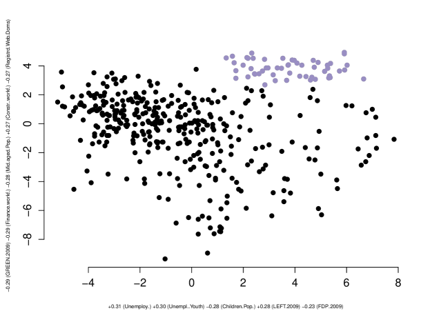
Exploration without prior background knowledge

We start with unguided data exploration where we have no prior knowledge about the data and our interest is as generic as possible. In this case $\mathcal{T}_{u}=\emptyset$ and as the hypothesis tilings we use $\mathcal{T}_{E_{1}}$, where all rows and columns belong to the same tile (fully-constrained tiling), and $\mathcal{T}_{E_{2}}$, where all columns form a tile of their own (fully unconstrained tiling). Our hypothesis pair is then $\mathcal{H}_{E,\emptyset}=\langle\emptyset+\mathcal{T}_{E_{1}},\emptyset+\mathcal{T}_{E_{2}}\rangle$.

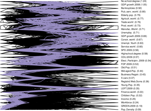
We then consider the view of the data (Figure 8) which is maximally informative, that is, in which the two distributions parametrised by the hypothesis pair $\mathcal{H}_{E,\emptyset}$ differ the most. We observe that there is some structure visible in this view. In order to investigate the characteristics of the data points corresponding to different patterns in the german data, we first choose to focus on the set of points in the upper right corner, marked with purple in Figure 8. Our selection, denoted by Selection 1, corresponds to rural districts in Eastern Germany (see Table 3). We also consider the parallel coordinates plot of the data, shown in Figure 9. This plot shows the 32 real-valued attributes in the data. The currently selected points (Selection 1) are shown in purple while the rest of the data is shown in black. The number in parentheses following each variable name is the ratio of the standard deviation of the selection and the standard deviation of all data. If this number is small we can conclude that the values for a particular attribute are homogeneous inside the selection (behave similarly). Based on the parallel coordinates plot in Figure 9 we observe that there is little support for the Green party and a high support for the Left party in these districts.

	Region				Type
Selection	North	South	West	East	Urban	Rural
Selection 1	0	0	0	54	0	54
Selection 2	10	7	21	22	60	0

Table 3: Distribution of the Region and Type attributes for Selection 1 and Selection 2 in the german data set.

Figure 10: The most informative view of the german data set with respect to $\mathcal{H}_{E,\{t\}}$. Black filled circles show the data points; the selected points, that is, Selection 2 are shown in orange. The points corresponding to Selection 1 from the previous exploration step are shown in purple. The $x$ and $y$ axis labels show the five attributes with the largest absolute values in each projection vector.

Figure 11: Parallel coordinates plot of the german data set with Selection 2 of Figure 10 highlighted in orange. See the caption of Figure 9 for an explanation of the semantics of the plot.

We next add a tile constraint $t$ for the items in the observed pattern where the columns (attributes) are chosen as described in Section 2.4 using a threshold value $\tau=2/3$. Thus, we select those attributes for which the standard deviation ratio, that is, the number in parentheses in Figure 9, is below the threshold. The hypothesis pair is then updated to take into account the newly added tile, that is, we consider $\mathcal{H}_{E,\{t\}}=\langle\{t\}+\mathcal{T}_{E_{1}},\{t\}+\mathcal{T}_{E_{2}}\rangle$.

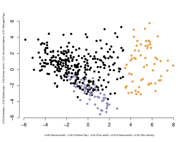
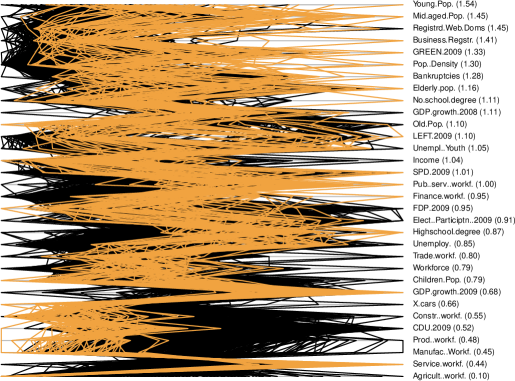
The most informative view displaying differences of the distributions parametrised by $\mathcal{H}_{E,\{t\}}$ is shown in Figure 10. Now, Selection 1 (shown in purple for illustration purposes) is no longer as clearly visible in Figure 10 as it is in the first view. This is expected, since this pattern has been accounted for in the distributions parametrised using $\mathcal{H}_{E,\{t\}}$. We now focus on investigating the sparse region of points shown in orange in Figure 10 (Selection 2). By inspecting the class attributes of this selection we learn that these items correspond to urban districts (see Table 3) in all regions. Based on the parallel coordinates plot shown in Figure 11 we conclude that these districts are characterised by a low fraction of agricultural workforce and a high amount of service workforce, both expected in urban districts. We also notice that these districts have had a higher GDP growth in 2009 and that it appears that the amount of votes for the CDU party in these districts was quite low.

Exploration with a specific hypothesis

Next, we focus on a more specific hypothesis involving only a subset of rows and attributes. In particular, we want to investigate a hypothesis concerning the relations between certain attribute groups in rural areas. We hence define our hypothesis pair as follows. As the subset of rows $R$ we choose all 298 districts that are of the type rural. We then consider a subset of the attributes $C=C_{1}\cup C_{2}\cup C_{3}\cup C_{4}$ partitioned into four groups. The first attribute group ($C_{1}$) consists of the voting results for the political parties in 2009. The second attribute group ($C_{2}$) describes demographic properties such as the fraction of elderly people, old people, middle aged people, young people, and children in the population. The third group ($C_{3}$) contains attributes describing the workforce in terms of the fraction of the different professions such as agriculture, production, or service. The fourth group ($C_{4}$) contains attributes describing the level of education, unemployment and income. The attribute groupings are listed in Table 4. Thus, we here want to investigate relations between different attribute groups, ignoring the relations inside the groups.

We form the hypothesis pair $\mathcal{H}_{F,\emptyset}=\langle\emptyset+\mathcal{T}_{F_{1}},\emptyset+\mathcal{T}_{F_{2}}\rangle$, where $\mathcal{T}_{F_{1}}$ consists of a tile spanning the rows in $R$ and the columns in $C$ whereas $\mathcal{T}_{F_{2}}$ consists of four tiles: $t_{i}=(R,C_{i})$, $i\in\{1,2,3,4\}$. Looking at the view in which the distributions parametrised by the pair $\mathcal{H}_{F,\emptyset}$ differ the most, shown in Figure 12(a), we find two clear clusters corresponding to a division of the districts into those located in the East, and those located elsewhere. We could also have used our already observed background knowledge of Selection 1, by considering the hypothesis pair $\mathcal{H}_{F,\{t\}}=\langle\{t\}+\mathcal{T}_{F_{1}},\{t\}+\mathcal{T}_{F_{2}}\rangle$, where $t$ is the tile defined earlier for Selection 1. For this hypothesis pair, the most informative view is shown in Figure 12(b), which clearly is different to Figure 12(a), since we already were aware of the relations concerning the rural districts in the East and this was included in our background knowledge.

Group	Attributes
$\bm{C_{1}}$	LEFT.2009, CDU.2009, SPD.2009, FDP.2009, GREEN.2009
$\bm{C_{2}}$	Elderly.pop., Old.Pop., Mid.aged.Pop., Young.Pop., Children.Pop.
$\bm{C_{3}}$	Agricult..workf., Prod..workf., Manufac..Workf., Constr..workf.,
	Service.workf., Trade.workf., Finance.workf., Pub..serv..workf.
$\bm{C_{4}}$	Highschool.degree, No.school.degree, Unemploy., Unempl..Youth, Income

Table 4: Column groups in the focus tile in the exploration of the german data set.

(a)	(b)

Figure 12: Views of the german data set corresponding to the hypothesis pairs (a) $\mathcal{H}_{F,\emptyset}$ and (b) $\mathcal{H}_{F,\{t\}}$. Data points inside the focus area are shown using filled circles ($\bullet$) and points outside the focus area are shown using hollow circles ($\circ$). The $x$ and $y$ axis labels show the five attributes with the largest absolute values in each projection vector.

	$\bm{\mathcal{H}_{E,\emptyset}}$	$\bm{\mathcal{H}_{E,\{t\}}}$	$\bm{\mathcal{H}_{F,\emptyset}}$	$\bm{\mathcal{H}_{F,\{t\}}}$
$\bm{v_{E,\emptyset}}$	8.831	4.211	1.921	1.195
$\bm{v_{E,\{t\}}}$	8.105	8.875	1.198	1.133
$\bm{v_{F,\emptyset}}$	4.879	2.241	2.958	1.193
$\bm{v_{F,\{t\}}}$	1.759	1.973	1.663	1.762
$\bm{v_{\mathrm{pca}}}$	8.831	4.211	1.921	1.195
$\bm{v_{\mathrm{ica}}}$	0.005	0.005	1.000	0.999

Table 5: The value of the gain $G(v,\mathcal{H})$ for different projection vectors $v$ and hypothesis pairs $\mathcal{H}$.

Comparison to PCA and ICA

To demonstrate the utility of the views shown, we compute values of the gain function as follows. We consider our four hypothesis pairs $\mathcal{H}_{E,\emptyset}$, $\mathcal{H}_{E,\{t\}}$, $\mathcal{H}_{F,\emptyset}$, and $\mathcal{H}_{F,\{t\}}$. For each of these pairs, we denote the direction in which the two distributions differ most in terms of the variance (solutions to Equation (2)) by $v_{E,\emptyset}$, $v_{E,\{t\}}$, $v_{F,\emptyset}$, and $v_{F,\{t\}}$, respectively. We then compute the gain $G(v,\mathcal{H})$ for each $v\in\{v_{E,\emptyset},v_{E,\{t\}},v_{F,\emptyset},v_{F,\{t\}}\}$ and $\mathcal{H}\in\{\mathcal{H}_{E,\emptyset},\mathcal{H}_{E,\{t\}},\mathcal{H}_{F,\emptyset},\mathcal{H}_{F,\{t\}}\}$. For comparison, we also compute the first principal component analysis (PCA) and independent component analysis (ICA) (Hyvärinen, 1999) projection vectors, denoted by $v_{\mathrm{pca}}$ and $v_{\mathrm{ica}}$, respectively, and calculate the gain for different hypothesis pairs using these. For ICA, we use the log-cosh $G$ function and default parameters of the R package fastICA. The results are presented in Table  5. We find that the gain is always the highest when the projection vector matches the hypothesis pair (highlighted in the table), as expected. This shows that the views presented are indeed the most informative ones given the current background knowledge and the hypothesis pair being investigated. We also notice that the gain for PCA is equal to that of unguided data exploration, as expected by Theorem 11. When some background knowledge is used or if we investigate a particular hypothesis, the views with PCA or ICA objectives are less informative than the one obtained using our framework. The gains close to zero for the ICA objective are directions in which the variance of the more constrained distribution is small due to, for example, linear dependencies in the data.

3.4 Exploration of the Accident Data Set

Due to the preprocessing, several columns in the accident data set are used to encode the distinct categorical values in the original data. If we now want to explore relationships between the original variables, we can define a hypothesis pair, in which columns corresponding to the same categorical attribute are grouped together. We can thus investigate relations between attribute groups, ignoring relations inside the groups.

Group	Attribute	# Values	Interpretation
$C_{1}$	AM1LK	14	Occupation of victim
$C_{2}$	EUSEUR	8	Days lost (severity of the accident)
$C_{3}$	IKAL	12	Age of victim (5-year bins, except 0–14 and
			$>$65 years)
$C_{4}$	NUORET	4	Age of victim (0–15, 16–17, 18–19, and $>$19 years)
$C_{5}$	RUUMIS	33	Injured body part
$C_{6}$	POIKKEA	10	Deviation before accident
$C_{7}$	SATK	12	Month of accident
$C_{8}$	SUKUP	2	Gender
$C_{9}$	TOLP	22	Main industry category
$C_{10}$	TPISTE	4	Workstation
$C_{11}$	TYOSUOR	9	Specific physical activity
$C_{12}$	TYOTEHT	31	Work done at the time of accident
$C_{13}$	VAHITAP	16	Contact-mode of injury
$C_{14}$	VAHTY	2	Accident class
$C_{15}$	VAMMAL	13	Type of injury
$C_{16}$	VPAIVA	7	Week day of accident
$C_{17}$	VUOSI	12	Year of accident

Table 6: Column groups in the focus tile in the exploration of the accident data set. For each attribute there are ‘# Values’ columns in the data set which are grouped together in the hypothesis tilings

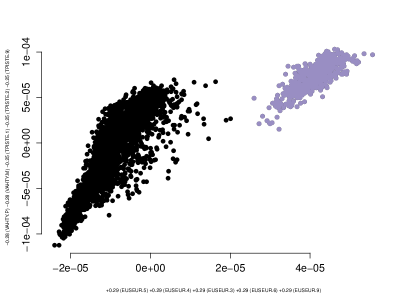
We define the hypothesis pair as follows. As the subset of rows $R$ we choose all the 3000 rows in the accident data set. We then consider a subset of the attributes $C=C_{1}\cup C_{2}\cup\cdots\cup C_{17}$, where a summary of the attribute groupings $C_{1},\ldots,C_{17}$ is provided in Table 6. The hypothesis pair is then $\mathcal{H}_{A,\emptyset}=\langle\emptyset+\mathcal{T}_{A_{1}},\emptyset+\mathcal{T}_{A_{2}}\rangle$, where $\mathcal{T}_{A_{1}}$ consists of a tile spanning all rows in $R$ and all columns in $C$ whereas $\mathcal{T}_{A_{2}}$ consists of tiles: $t_{i}=(R,C_{i})$, $i\in\{1,\ldots,17\}$. The view in which the distributions parametrised by $\mathcal{H}_{A,\emptyset}$ differ the most is shown in Figure 13(a). Here we observe two clear clusters. We select the points shown in purple and observe that these data points correspond to accidents happening during travel to work (vahty.m). Also, the attributes tpiste, tyoteht, tyosuor, poikkea, and vahitap (all related to the type of work or the place of work in which the accident occurred) have missing values (–) here, which is natural when an accident happens during travelling to work. The points in the complement of the purple selection on the other hand correspond to accidents happening in the workplace (vahty.p).

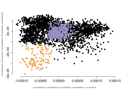
Next, we add a tile $t_{A}$ with the selection of purple points in Figure 13(a) as the set of rows and all columns in the accident data as the set of columns to incorporate our knowledge concerning these points into the exploration. We proceed to consider the updated hypothesis pair $\mathcal{H}_{A,\{t_{A}\}}=\langle\{t_{A}\}+\mathcal{T}_{A_{1}},\{t_{A}\}+\mathcal{T}_{A_{2}}\rangle$. The most informative view for this hypothesis pair is shown in Figure 13(b). For illustration purposes we show in purple the same selection of rows in data as in Figure 13(a). We can now select, for example, the data points shown in orange in Figure 13(b) for further inspection. This selection corresponds to accidents in the workplace (vahty.p) which happened mainly to women (sukup.n) over 19 years old (nuoret.4), resulting in 31–90 days of absence from work (euseur.9).

(a)	(b)

Figure 13: Views of the accident data set corresponding to the hypothesis pairs (a) $\mathcal{H}_{A,\emptyset}$ and (b) $\mathcal{H}_{A,\{t_{A}\}}$. Filled circles show the data points; the selected points are marked with purple/orange, see description in the text. The $x$ and $y$ axis labels show the five attributes with the largest absolute values in each projection vector.

4 Conclusions

In this paper we propose an interactive visual data exploration framework integrating the user’s background knowledge (increasing iteratively during the exploration) and the user’s current exploration interests in a principled way. We provide an efficient implementation of this method using constrained randomisation. Furthermore, we also extended PCA to work seamlessly with the framework in the case of real-valued data sets.

Typical real-world data sets, for instance those empirically investigated in this paper, contain a vast number of interesting patterns. The goal of the data analyst is to find interesting relations in the data. If automated analysis methods are used to extract patterns, it means that the patterns must be specified in advance to be used in conjunction with some data mining algorithm. Specifying patterns in advance is clearly nontrivial when there is a multitude of variable combinations that must be taken into account. Furthermore, if patterns are only extracted based on a priori specifications it is not possible to use insights obtained during the exploration to steer further exploration.

It is here where the power of human-guided data exploration lies. A non-interactive data mining method is restricted to either show generic features of the data—which may already be obvious to an expert—or output unusably many patterns, which is a typical problem, for example, in frequent pattern mining (there are easily too many patterns for the user to absorb). Our framework solves this problem: by integrating the human’s background knowledge and focus—formulated as mathematically defined hypotheses—we can at the same time guide the search towards topics interesting to the user at any particular moment while taking the user’s prior knowledge into account in an understandable and efficient way. Hence, the framework described in this paper makes it possible to interactively and efficiently explore relations between attributes in the data through a conceptually simple paradigm where the relations are encoded using tile constraints. This exploration framework allows the data analyst to use his or her innate pattern recognition skills to spot complex patterns, instead of having to specify them in advance. As demonstrated in our empirical evaluation of two real-world data sets, the proposed interactive exploration framework allows us to find interesting patterns and hence to make sense of the relations in the data.

Our work contains implicit assumptions about the human cognitive processing, such that the user’s knowledge can be modelled using a background distribution. The validity of these assumptions is an interesting topic for future research. For example, the order in which different relations are observed probably matters to a real user, whereas our formulation is invariant under ordering of the relations. Also, the user is probably not able to model very fine-grained distributions, while our mathematical formulation of the background distribution can become extremely complex when the number of constraints grows.

As a potential direction for future work we consider the extension of the proposed method to understand classifiers or regression functions in addition to static data. Extending the ideas used here to different data types such as, for example, time series, is also worth investigating. Finding an efficient algorithm that could find a sparse solution to the optimisation problem of Equation (2) would also be an interesting problem. To the best of our knowledge, no such solution is readily available. We note that the solutions for sparse PCA are not directly applicable here: sparse PCA would indeed give a sparse variant of the vector $w$ in Theorem 10. However, this would not result in a sparse $v_{\mathcal{H}}=Ww$. Furthermore, we plan to study how to incorporate in our framework a scheme for evaluating the statistical significance of the visually observed patterns.

In our work, we chose to use a linear projection and showed that our method reduces to PCA at the limit of generic objectives and no background information. We showed that linear projections can be computed efficiently for arbitrary background knowledge and objectives (expressed in our tile notation). We could, however, in principle replace the linear projection by a non-linear embedding that would in the same way show differences between the hypothesis pairs. In their recent work, Kang et al. (2020) presented a variant of t-SNE that can be used to produce informative visualisations with the background information parametrised by a partition of data points into known classes. Their method is not applicable to generic tile constraints, but it might be possible to use their ideas to develop a non-linear embedding that would work with generic tile constraints, in which case the resulting visualisation method could be used as a drop-in replacement for the linear projection presented in this paper.

In this paper we have implicitly assumed that the exploration takes place in one exploration session by a single user. In practical applications it might make sense to incorporate data constraints learned on earlier exploration sessions or by other users into the model, and to modify the hypotheses based on the insights gained.

Finally, we have implemented an open source R package that allows us to simulate interactive visual data exploration using our framework. The framework is available under an open source license from https://github.com/edahelsinki/corand/ and it includes, in addition to the code needed to run the experiments in this paper, an interactive web-based interface prototype. We have also earlier released a preliminary prototype called tiler (Henelius et al., 2018), which includes the tile-based constrained randomisation approach, but does not implement the dimensionality reduction method presented in this work.

Acknowledgments

We thank Buse Gul Atli for discussions and contributions to the preprint (Puolamäki, Oikarinen, Atli, and Henelius, 2018). We thank the Finnish Workers’ Compensation Center for the access to the accident data. This work was supported by the Academy of Finland (decisions 326280 and 326339).

A Algorithm for merging tiles

Merging a new tile into a tiling where all tiles are non-overlapping can be done efficiently using Algorithm 1. We assume that the starting point is always a non-overlapping set of tiles and hence we only need to consider the overlap that the new tile has with the tiles in the tiling. This is similar to the merging of statements considered by Kalofolias et al. (2016). The algorithm has two steps. Let $\mathcal{T}$ be the current tiling and $t=(R,C)$ the new tile to be added. In the first step (lines 1–11) we identify the tiles in $\mathcal{T}$ with which $t$ overlaps, and in the second step (lines 12–17) we resolve (merge) the overlap between $t$ and the tiles identified in the previous step.

The first step proceeds as follows. An empty hash map is initialised (line 1) to be used to detect overlap between columns of the tiles in $\mathcal{T}$ and the new tile $t$. We proceed to iterate over each row $R$ in the new tile (lines 2–11). Since $\mathcal{T}$ is a tiling, all its tiles are non-overlapping. We can thus store $\mathcal{T}$ in a matrix of the same size as the data matrix where each element corresponds to the ID of the tile that covers that position. With a slight abuse of notation, $\mathcal{T}$ in the algorithm refers to such a matrix. Now, given a row $i\in R$ and a set of columns $C$ (line 3) we then get the IDs of the tiles on row $i$ with which $t$ overlaps. We store this in $K$. The hash map is used to detect if this row has been seen before, that is, whether $K$ is a key in $S$ (line 4). If this is the first time this row is seen, $K$ is used as the key for a new element in the hash map and $S(K)$ is initialised to be a tuple (line 5). Elements in this tuple are referred to by name, for instance, $S(K)_{\mathrm{rows}}$ gives the set of rows associated with the key $K$, while $S(K)_{\mathrm{id}}$ gives the set of tile IDs. On lines 6 and 7 we store the current row index $S(K)_{\mathrm{rows}}$ and the unique tile IDs $S(K)_{\mathrm{id}}$ in the tuple. If the row was seen before, the row set associated with these tile IDs is updated (line 9). After this first step, the hash map $S$ contains tuples of the form (rows, id) where id specifies the IDs of the tiles with which $t$ overlaps at the rows specified by rows.

In the second step of the algorithm (lines 12–17), we first determine the currently largest tile ID in use (line 12). After this we iterate over the tuples in the hash map $S$. For each tuple we must update the tiles having IDs $S(K)_{\mathrm{id}}$ and on line 14 we hence find the columns associated with these tiles. After this, the IDs of the affected overlapping tiles are updated (line 15), and the tile ID counter is incremented (line 16). Finally, the updated tiling is returned on line 18. The time complexity of the tile merging algorithm is $\mathcal{O}{(nm)}$.

1

input : Tiling $\mathcal{T}$ as an $n\times m$ data matrix where an element is the ID of the tile to which it belongs, and a tile $t=(R,C)$.

output : $\mathcal{T}+\{t\}$ (the tiling in which $\mathcal{T}$ is merged with $t$).

2

3$S\leftarrow\texttt{HashMap}$;

4

5for $i\in R$ do

6       $K\leftarrow\mathcal{T}(i,C)$;

7       if $K\notin\texttt{keys}(S)$ then

8             $S(K)\leftarrow\texttt{Tuple}$;

9             $S(K)_{\mathrm{rows}}\leftarrow\{i\}$;

10             $S(K)_{\textrm{id}}\leftarrow\texttt{unique}(\mathcal{T}(i,C))$;

11            

12       else

13             $S(K)_{\textrm{rows}}\leftarrow S(K)_{\textrm{rows}}\cup\{i\}$;

14            

15       end if

16      

17 end for

18

19$p_{\mathrm{max}}\leftarrow\max(\mathcal{T}(R,C))$;

20 for $K\in\texttt{keys}(S)$ do

21       $C^{\prime}=\left\{c\mid\mathcal{T}(S(K)_{\mathrm{rows}},c)\in S(K)_{\textrm{id}}\right\}$ ;

22       $\mathcal{T}\left(S(K)_{\textrm{rows}},C^{\prime}\right)\leftarrow p_{\mathrm{max}}+1$ ;

23       $p_{\mathrm{max}}\leftarrow p_{\mathrm{max}}+1$;

24      

25 end for

return $\mathcal{T}$

Algorithm 1 Merging a tile $t$ with the tiles in a tiling $\mathcal{T}$. The function HashMap denotes a hash map. The value in a hash map $H$ associated with a key $x$ is $H(x)$ and $\texttt{keys}(H)$ gives the keys of $H$. The function Tuple creates a (named) tuple. An element $a$ in a tuple $w=(\mathrm{a},\mathrm{b})$ is accessed as $w_{\mathrm{a}}$. The function unique returns the unique elements of an array.

References

- Boley et al. (2013) Mario Boley, Michael Mampaey, Bo Kang, Pavel Tokmakov, and Stefan Wrobel. One click mining—interactive local pattern discovery through implicit preference and performance learning. In ACM SIGKDD Workshop on Interactive Data Exploration and Analytics (IDEA), pages 27–35, 2013.
- Chau et al. (2011) Duen Horng Chau, Aniket Kittur, Jason I. Hong, and Christos Faloutsos. Apolo: making sense of large network data by combining rich user interaction and machine learning. In SIGCHI Conference on Human Factors in Computing Systems, pages 167–176, 2011.
- Chirigati et al. (2016) Fernando Chirigati, Harish Doraiswamy, Theodoros Damoulas, and Juliana Freire. Data polygamy: the many-many relationships among urban spatio-temporal data sets. In International Conference on Management of Data (SIGMOD/PODS), pages 1011–1025. ACM, 2016.
- De Bie (2011a) Tijl De Bie. An information theoretic framework for data mining. In ACM SIGKDD International Conference on Knowledge Discovery and Data Mining, pages 564–572. ACM, 2011a.
- De Bie (2011b) Tijl De Bie. Maximum entropy models and subjective interestingness: an application to tiles in binary databases. Data Mining and Knowledge Discovery, 23(3):407–446, 2011b.
- De Bie (2013) Tijl De Bie. Subjective interestingness in exploratory data mining. In International Symposium on Intelligent Data Analysis (IDA), pages 19–31, 2013.
- De Bie et al. (2016) Tijl De Bie, Jefrey Lijffijt, Raúl Santos-Rodriguez, and Bo Kang. Informative data projections: a framework and two examples. In European Symposium on Artificial Neural Networks, Computational Intelligence and Machine Learning, pages 635–640, 2016.
- Dzyuba and van Leeuwen (2013) Vladimir Dzyuba and Matthijs van Leeuwen. Interactive discovery of interesting subgroup sets. In International Symposium on Intelligent Data Analysis (IDA), pages 150–161, 2013.
- Fisher (1936) R. A. Fisher. The use of multiple measurements in taxonomic problems. Annals of Eugenics, 7:179–188, 1936.
- Hanhijärvi et al. (2009) Sami Hanhijärvi, Markus Ojala, Niko Vuokko, Kai Puolamäki, Nikolaj Tatti, and Heikki Mannila. Tell me something I don’t know: randomization strategies for iterative data mining. In ACM SIGKDD International Conference on Knowledge Discovery and Data Mining, pages 379–388. ACM, 2009.
- Henelius et al. (2018) Andreas Henelius, Emilia Oikarinen, and Kai Puolamäki. Tiler: software for human-guided data exploration. In Proceedings of the Joint European Conference on Machine Learning and Knowledge Discovery in Databases (ECML-PKDD), pages 672–676. Springer, 2018.
- Hyvärinen (1999) Aapo Hyvärinen. Fast and robust fixed-point algorithms for independent component analysis. IEEE Transactions on Neural Networks, 10(3):626–634, 1999.
- Kalofolias et al. (2016) Janis Kalofolias, Esther Galbrun, and Pauli Miettinen. From sets of good redescriptions to good sets of redescriptions. In International Conference on Data Mining (ICDM), pages 211–220. IEEE, 2016.
- Kang et al. (2016a) Bo Kang, Jefrey Lijffijt, Raúl Santos-Rodríguez, and Tijl De Bie. Subjectively interesting component analysis: Data projections that contrast with prior expectations. In ACM SIGKDD International Conference on Knowledge Discovery and Data Mining, pages 1615–1624, 2016a.
- Kang et al. (2016b) Bo Kang, Kai Puolamäki, Jefrey Lijffijt, and Tijl De Bie. A tool for subjective and interactive visual data exploration. In Joint European Conference on Machine Learning and Knowledge Discovery in Databases (ECML-PKDD), pages 3–7. Springer, 2016b.
- Kang et al. (2020) Bo Kang, Darío Garcría García, Jefrey Lijffijt, Raúl Santos-Rodríguez, and Tijl De Bie. Conditional t-SNE: more informative t-SNE embeddings. Machine Learning, 2020.
- Kessy et al. (2018) Agnan Kessy, Alex Lewin, and Korbinian Strimmer. Optimal whitening and decorrelation. The American Statistician, 72(4):309–314, 2018.
- Lijffijt et al. (2014) Jefrey Lijffijt, Panagiotis Papapetrou, and Kai Puolamäki. A statistical significance testing approach to mining the most informative set of patterns. Data Mining and Knowledge Discovery, 28(1):238–263, 2014.
- Paurat et al. (2014) Daniel Paurat, Roman Garnett, and Thomas Gärtner. Interactive exploration of larger pattern collections: a case study on a cocktail dataset. In ACM SIGKDD Workshop on Interactive Data Exploration and Analytics (IDEA), pages 98–106, 2014.
- Puolamäki et al. (2010) Kai Puolamäki, Panagiotis Papapetrou, and Jefrey Lijffijt. Visually controllable data mining methods. In IEEE International Conference on Data Mining Workshops, pages 409–417, 2010.
- Puolamäki et al. (2016) Kai Puolamäki, Bo Kang, Jefrey Lijffijt, and Tijl De Bie. Interactive visual data exploration with subjective feedback. In Joint European Conference on Machine Learning and Knowledge Discovery in Databases (ECML-PKDD), pages 214–229. Springer, 2016.
- Puolamäki et al. (2018) Kai Puolamäki, Emilia Oikarinen, Buse Gul Atli, and Andreas Henelius. Human-guided data exploration using randomisation. arXiv preprint arXiv:1805.07725, 2018.
- Puolamäki et al. (2018) Kai Puolamäki, Emilia Oikarinen, Bo Kang, Jefrey Lijffijt, and Tijl De Bie. Interactive visual data exploration with subjective feedback: an information-theoretic approach. In IEEE International Conference on Data Engineering (ICDE), pages 1208–1211, 2018.
- R Core Team (2018) R Core Team. R: A Language and Environment for Statistical Computing. R Foundation for Statistical Computing, Vienna, Austria, 2018. URL https://www.R-project.org/.
- Ruotsalo et al. (2015) Tuukka Ruotsalo, Giulio Jacucci, Petri Myllymäki, and Samuel Kaski. Interactive intent modeling: information discovery beyond search. Communications of the ACM, 58(1):86–92, 2015.
- Tukey (1977) John W. Tukey. Exploratory Data Analysis. Addison-Wesley, 1977.
- van Leeuwen and Cardinaels (2015) Matthijs van Leeuwen and Lara Cardinaels. VIPER—visual pattern explorer. In Joint European Conference on Machine Learning and Knowledge Discovery in Databases (ECML-PKDD), pages 333–336, 2015.
- Vartak et al. (2015) Manasi Vartak, Sajjadur Rahman, Samuel Madden, Aditya Parameswaran, and Neoklis Polyzotis. SeeDB: efficient data-driven visualization recommendations to support visual analytics. In Proceedings VLDB Endowment, volume 8(3), pages 2182–2193, 2015.
- Wilkinson et al. (2005) Leland Wilkinson, Anushka Anand, and Robert Grossman. Graph-theoretic scagnostics. In Proceedings of the 2005 IEEE Symposium on Information Visualization (INFOVIS), page 21. IEEE, 2005.