Tree-based Inference of Species Interaction Network from Abundance Data

Summary

1. The behavior of ecological systems mainly relies on the interactions between the species it involves. We consider the problem of inferring the species interaction network from abundance data. To be relevant, any network inference methodology needs to handle count data and to account for possible environmental effects. It also needs to distinguish between direct interactions and indirect associations and graphical models provide a convenient framework for this purpose.
2. We introduce a generic statistical model for network inference based on abundance data. The model includes fixed effects to account for environmental covariates and sampling efforts, and correlated random effects to encode species interactions. The inferred network is obtained by averaging over all possible tree-shaped (and therefore sparse) networks, in a computationally efficient manner. An output of the procedure is the probability for each edge to be part of the underlying network.
3. A simulation study shows that the proposed methodology compares well with state-of-the-art approaches, even when the underlying graph strongly differs from a tree. The analysis of two datasets highlights the influence of covariates on the inferred network.
4. Accounting for covariates is critical to avoid spurious edges. The proposed approach could be extended to perform network comparison or to look for missing species.

Key-words:

abundance data, covariates adjustment, EM algorithm, graphical models, matrix tree theorem, Poisson log-Normal model, species interaction network

1 Introduction

There is a growing awareness of biotic interactions being crucial components of biodiversity and relevant descriptors of ecosystems (Valiente-Banuet et al., 2015; Jordano, 2016). Such interactions can be conveniently represented by networks, which have been increasingly studied and used in recent years for describing and understanding living systems in ecology (Poisot et al., 2016), microbiology (Faust and Raes, 2012) or genomics (Evans et al., 2016). Observing species interactions is a laborious task which restricts them to certain categories (e.g. trophic, pollination), while many other mutualistic and/or antagonistic interactions may be hard to observe and key in the system organization (e.g. communication, shelter sharing). Many efforts have been devoted in the last decade to get a more complete picture of the biotic interactions existing between species living in the same niche.

Network reconstruction.

A first attempt consists in using observed interactions to predict other possible links based on species traits matching (see e.g. Olito and Fox, 2015; Bartomeus et al., 2016; Weinstein and Graham, 2017; Graham and Weinstein, 2018). The interaction strength can also be predicted (Wells and O’Hara, 2013). This can be viewed as a prediction task, and modern approaches arising from signal processing and machine learning have been also proposed (Desjardins-Proulx et al., 2017; Stock et al., 2017; Dallas et al., 2017). We name these approaches network reconstruction to distinguish them from network inference, which is the problem we consider in this article.

Network inference.

Network inference approaches also aim at retrieving the interactions among species, but do not rely on observed interactions and therefore, remain agnostic as for their type. Such approaches have been developed in many domains ranging from cell biology (Friedman, 2004, to infer gene regulatory networks) to neurosciences (Zhu and Cribben, 2018, to deciphere brain connectivity structures). In ecology, it will typically aim at inferring the set of biotic interactions linking species from the same guild. As summarized in Fig. 1, network inference takes as input measures on species at similar sites, and returns a network of species direct interactions. The importance of distinguishing between direct interaction and indirect association between species is explained in Popovic et al. (2019). To be accurate, network inference must account for environmental covariates to prevent the inference of spurious interactions resulting from abiotic effects. Fig. 1 illustrates this phenomenon: ($c$) corresponds to the case where two species (1 and 4) are not in direct interaction, but are affected by the variations of the same environmental covariate $x$. ($d$) displays the network when $x$ is not accounted for: a spurious edge appears between these two species.

date site apr93 km03 apr93 km03 apr93 km03 apr93 km03 apr93 km17 apr93 km17 ⋮ ⋮		EFI ELA GDE GME HFA 71 1 5 6 0 118 2 3 0 0 69 0 6 2 0 56 0 0 0 0 0 1 1 0 0 0 0 2 0 0 ⋮ ⋮ ⋮ ⋮ ⋮
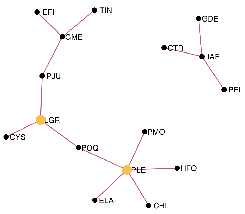
($a$) covariates		($b$) species abundances		($c$) inferred network

Figure 1: Aim of species interaction network inference from abundance data. Data sample from the Fatala river dataset (see Section 2.3.4).

Joint species distribution models.

The rational between network inference is that interactions between species must affect their joint distribution in a series of similar sites. Such approaches necessarily rely on a joint species distribution model (JSDM), as opposed to species distribution models (Elith and Leathwick, 2009) where species are traditionally considered as disconnected entities. A JSDM is a probabilistic model describing the species simultaneous presence/absence (Harris, 2015; Ovaskainen et al., 2017) or joint abundances (Popovic et al., 2018, 2019). An important feature of JSDMs is to include environmental covariates to account for abiotic interactions.
Recently, latent variable models have received attention in community ecology as they provide a convenient way to model the dependence structure between species (Warton et al., 2015). The JSDM proposed by Popovic et al. (2018, 2019) involves a latent layer. So does the Poisson log-Normal model (PLN, Aitchison and Ho, 1989), which combines generalized linear models to account for covariates and offsets, and a Gaussian latent structure to describe the species interactions. It can be seen as a multivariate mixed model, in which correlated random effects encode the dependency between the species abundances.

&          ($a$) connected ($b$) disconnected ($c$) with covariate ($d$) missing covariate

Figure 2: Examples of graphical models.

Graphical models: a generic framework for network inference.

Although they describe the dependence structure between the distributions of all the species from a same niche, JSDM are not sufficient to perform network inference as they do not distinguish indirect associations from direct interactions (Dormann et al., 2018). Graphical models (Lauritzen, 1996) provide a probabilistic framework to do so and, in the same time, a formal definition of the network to be inferred. This formalism is therefore especially appealing for the inference of species interaction networks (Popovic et al., 2019). In an undirected graphical model (which is the same as a Markov random field: Clark et al., 2018), two species are connected if they are dependent conditional on all other species, that is if the variations of their respective abundances would still be correlated if ever both the environmental conditions and the abundances of all other species were kept fixed. Two species are unconnected if they are independent conditional on all other species: the observed correlation between them only results from a series of links with other species (Morueta-Holme et al., 2016). Fig. 1 illustrates the concept of conditional dependence/independence with toy graphical models. In ($a$), the network is connected so all species are interdependent: an association exists between any two of them. However, 1 is only directly interacting with 2 which mediates its association with 3 and 4: 1 is independent from them conditional on 2. In ($b$), the network is disconnected: species 4 is independent from all others. This illustrates that graphical models enjoy all the desirable properties to represent interactions between species in an interpretable manner, so that they can be used as the mathematical counterpart of species interaction networks.

Network inference: the general problem.

Network inference methods attempts to retrieve the graphical model underlying the distribution of observed data. In every domains, network inference is impeded by the huge number of possible graphs for a given set of nodes, which increases super-exponentially with the latter (more than $10^{13}$ undirected graphs can be drawn between 10 nodes, and more than $10^{57}$ between 20). The exploration of the graph space is therefore intractable from a combinatorial point of view. To reduce the search space, a common and reasonable assumption is that a relatively small fraction of species pairs are in direct interaction: the network is sparse. In the case of continuous observations, one of the most popular approach is the graphical lasso (glasso: Friedman et al., 2008a) which takes advantage of the properties of Gaussian graphical models (GGM) to efficiently infer a sparse network. Alternatively, tree-based approaches have been proposed: Chow and Liu (1968) first made the too stringent assumption that the network is made of a single spanning tree (that is connecting all nodes without any loop, as in Fig. 1). More recent approaches introduced by Meilă and Jaakkola (2006) and Kirshner (2008) rely on efficient algebraic tools to average over all possible tree-structured graphical models. The inferred network resulting from such an averaging procedure is not restricted to be a tree: species or groups of species can be isolated (e.g. Fig. 1), and loops can appear (e.g. Fig. 1).

Network inference from species abundance data.

This work focuses on network inference based on abundance data, and not only their presence/absence (as considered in Ovaskainen et al., 2010; Clark et al., 2018). Network inference from species abundance measures is a notoriously difficult problem (Ulrich and Gotelli, 2010), not only because network inference is complex, but also because it has to account for the data specificities. Abundance data may spread over a wide range of values and often result from sampling efforts (sample and/or species-specific), making them difficult to compare. Obviously, count data do not directly fit the Gaussian framework but many network inference methods dedicated to abundance data actually rely on a latent Gaussian structure (see Section 2.3.1).

Contribution.

In the present work, we adopt a model-based approach to perform network inference from abundance data. To accommodate the data specificities we use a PLN model, which includes the over-dispersion of the observed counts as well as the sampling effort. Importantly, the PLN model allows to account for abiotic effects and avoid the detection of spurious interactions between species. As for the network inference, we adopt a tree-based approach (as opposed to Biswas et al., 2016, which also use a PLN model but resort to glasso), which provides a probability for each edge to be actually part of the underlying graphical model.

Outline.

We introduce the method EMtree, which combines two (variational) EM algorithms to estimate the model parameters. Importantly, our approach provides the probability for each possible edge to be part of the interaction network. We evaluate our approach on both synthetic and ecological datasets. An R package implementing EMtree is available on GitHub https://github.com/Rmomal/EMtree.

2 Material and methods

2.1 Model

Let us first describe the typical type of data we consider. We assume that $p$ species have been observed in $n$ sites and we denote $Y_{ij}$ the abundance of species $j$ in site $i$. The abundances are gathered in the $n\times p$ matrix ${\bf Y}$. We denote by ${\bf Y}_{i}$ the $i$th row of matrix ${\bf Y}$, which corresponds to the abundance vector collected in site $i$. We further assume that a vector of covariates ${\bf x}_{i}$ has been measured in each site $i$ and that all covariates are gathered in the $n\times d$ matrix ${\bf X}$. The sites are supposed to be independent.

Our aim is to decipher the dependency structure between the $p$ species, accounting for the effect of the environmental covariates encoded in ${\bf X}$. As explained above, ignoring environmental covariates is more than likely to result in spurious edges.

Mixed model.

To distinguish between covariates effects and species interactions, we consider a mixed model which states that each abundance $Y_{ij}$ has a (conditional) Poisson distribution

$$Y_{ij}\sim\mathcal{P}\left(\exp({\bf x}_{i}^{\intercal}{\bm{\theta}}_{j}+o_{ij}+Z_{ij})\right).$$ (1)

In model (1), $o_{ij}$ is the sample- and species-specific offset which accounts for the sampling effort. ${\bm{\theta}}_{j}$ is the vector of fixed regression coefficients measuring the effect of each covariate on species $j$ abundance. The regression part is similar to a general linear model as used in niche modeling (see e.g. Austin, 2007). $Z_{ij}$ is the random effect associated with species $j$ in site $i$. Importantly, the coordinates of the site-specific random vector ${\bf Z}_{i}=(Z_{i1},\dots Z_{ip})$ are not independant: the multivariate random term ${\bf Z}_{i}$ precisely accounts for the interactions that are not due to environmental fluctuations. For each site $i$, a vector ${\bf Z}_{i}$ is associated with the corresponding abundance vector ${\bf Y}_{i}$. The distribution given in Eq. (1) is over-dispersed as the Poisson parameter is itself random, which suits ecological modeling of abundance data (Richards, 2008).

We now describe the distribution of the latent vector ${\bf Z}_{i}$. To this aim, we adopt a version of Kirshner’s model (Kirshner, 2008), which states that a spanning tree $T$ is first drawn with probability

$$p(T)=\prod_{(j,k)\in T}\beta_{jk}/B,$$ (2)

where $(j,k)\in T$ means that the edge connecting species $j$ and $k$ is part of the tree $T$ and where $B$ is a normalizing constant. Each edge weight $\beta_{jk}$ controls the probability for the edge $(j,k)$ to be in the interaction network. Then for each site $i$, a vector ${\bf Z}_{i}$ is drawn independently with conditional Gaussian distribution $({\bf Z}_{i}\mid T)\sim\mathcal{N}(0,\Sigma_{T})$, where the subscript T means that the distribution of ${\bf Z}_{i}$ is faithful to $T$. When $T$ is a spanning tree, this faithfulness simply means this distribution can be factorized on the nodes and edges of $T$ as follows (see Kirshner, 2008):

$$p({\bf Z}_{i}\mid T)=\prod_{j=1}^{p}p(Z_{ij}|T)\prod_{(j,k)\in T}\psi_{jk}({\bf Z}_{i}),$$ (3)

where $\psi_{jk}({\bf Z}_{i})$ does not depend on $T$. This factorization means that each edge of $T$ corresponds to a species pair in direct interaction; all other pairs are conditionally independent. Experiments are independent, and in the sequel we consider the product of all $p({\bf Z}_{i})$ and use the simpler notation $\psi_{jk}=\prod_{i}\psi_{jk}({\bf Z}_{i})$ instead.

According to Eq. (2), each ${\bf Z}_{i}$ has a Gaussian distribution conditional on the tree $T$, so its marginal distribution is a mixture of Gaussians: ${\bf Z}_{i}\sim\sum_{T\in\mathcal{T}}p(T)\mathcal{N}(0,\Sigma_{T})$, where $\mathcal{T}$ is the set of all spanning trees. As a consequence, the joint distribution of the ${\bf Z}_{i}$ is modeled by a mixture of distributions with tree-shaped dependency structure. Besides, for all trees including the edge $(j,k)$, the estimate of the covariance term between the coordinates $j$ and $k$ is the same (see Lauritzen, 1996; Schwaller et al., 2019). Hence, we may define a global covariance matrix ${\bm{\Sigma}}$, filled with covariances that are each common to spanning trees containing a same edge. Each ${\bm{\Sigma}}_{T}$ is then built by extracting from ${\bm{\Sigma}}$ the covariances corresponding to the edges of $T$.

2.2 Inference with EMtree

We now describe how to infer the model parameters. We gather the edges weights $(\beta_{jk})_{jk}$ into the $p\times p$ matrix ${\bm{\beta}}$ and the vectors of regression coefficients into a $d\times p$ matrix ${\bm{\theta}}$. The $p\times p$ matrix ${\bm{\Sigma}}$ contains the variances and covariances between the coordinates of each latent vector ${\bf Z}_{i}$. Hence, the set of parameters to be inferred is $({\bm{\beta}},{\bm{\Sigma}},{\bm{\theta}})$.

Likelihood.

The model described above is an incomplete data model, as it involves two hidden layers: the random tree $T$ and the latent Gaussian vectors ${\bf Z}_{i}$. The most classical approach to achieve maximum likelihood inference in this context is to use the Expectation-Maximization algorithm (EM: Dempster et al., 1977). Rather than the likelihood of the observed data $p({\bf Y})$, the EM algorithm deals with the often more tractable likelihood $p(T,{\bf Z},{\bf Y})$ of the complete data (which consists of both the observed and the latent variables). It can be decomposed as

$$p_{{\bm{\beta}},{\bm{\Sigma}},{\bm{\theta}}}(T,{\bf Z},{\bf Y})=p_{{\bm{\beta}}}(T)\times p_{{\bm{\Sigma}}}({\bf Z}\;|\;T)\times p_{{\bm{\theta}}}({\bf Y}\;|\;{\bf Z}),$$ (4)

where the subscripts indicate on which parameter each distribution depends. Observe that the dependency structure between the species is only involved in the first two terms, whereas the third term only depends on the regression coefficients ${\bm{\theta}}$. We take advantage of this decomposition to propose a two-stage estimation algorithm. The first stage deals with the observed layer $p_{{\bm{\theta}}}({\bf Y}\;|\;{\bf Z})$, the second with the two hidden layers $p_{{\bm{\beta}}}(T)$ and $p_{{\bm{\Sigma}}}({\bf Z}\;|\;T)$. The network inference itself takes place in the second step.

Inference in the observed layer.

The variational EM (VEM) algorithm that provides an estimate of the regression coefficients matrix ${\bm{\theta}}$ is described in Appendix A.1 (along with a reminder on EM and VEM). It also provides the (approximate) conditional means $\operatorname*{\mathbb{E}}(Z_{ij}|{\bf Y}_{i})$, variances $\operatorname*{\mathbb{V}}(Z_{ij}|{\bf Y}_{i})$ and covariances $\operatorname*{\mathbb{C}\text{ov}}(Z_{ij},Z_{ik}|{\bf Y}_{i})$ required for the inference in the hidden layer. As a consequence, this first step provides the estimates $\widehat{{\bm{\theta}}}$ and $\widehat{{\bm{\Sigma}}}$.

Inference in the hidden layer.

The second step is dedicated to the estimation of ${\bm{\beta}}$. The EM algorithm actually deals with the conditional expectation of the complete log-likelihood, namely $\operatorname*{\mathbb{E}}\left(\log p_{{\bm{\beta}},{\bm{\Sigma}},{\bm{\theta}}}(T,{\bf Z},{\bf Y})\;|\;{\bf Y}\right)$. As shown in Appendix A.2, this reduces to

$$\operatorname*{\mathbb{E}}\left(\log p_{{\bm{\beta}},{\bm{\Sigma}},{\bm{\theta}}}(T,{\bf Z},{\bf Y})\;|\;{\bf Y}\right)\simeq\sum_{1\leq j<k\leq p}P_{jk}\log\left(\beta_{jk}\widehat{\psi}_{jk}\right)-\log B+\text{cst}$$ (5)

where $\widehat{\psi}_{jk}$ is the estimate of $\psi_{jk}$ defined in Eq. (3), and the ’cst’ term depends on ${\bm{\theta}}$ and ${\bm{\Sigma}}$ but not on ${\bm{\beta}}$. $P_{jk}$ is the approximate conditional probability (given the data) for the edge $(j,k)$ to be part of the network: $P_{jk}\simeq\operatorname*{\mathds{P}}\{(j,k)\in T\;|\;Y\}$. It is also shown in Appendix A.2 that $\widehat{\psi}_{jk}=(1-\widehat{\rho}_{jk}^{2})^{-n/2}$, where the estimated correlation $\widehat{\rho}_{jk}$ depends on the conditional mean, variance and covariances of the $Z_{ij}$’s provided by the first step. Eq. (5) is maximized via an EM algorithm iterating the calculation of the $P_{jk}$ and the maximization with respect to the $\beta_{jk}$:

Expectation step: Computing the $P_{jk}$ with tree averaging.

The conditional probability of an edge is simply the sum of the conditional probabilities of the trees that contain this edge. Hence, computing $P_{jk}$ amounts to averaging over all spanning trees. Fig. 1 illustrates the principle of tree averaging for a toy network with $p=4$ nodes. Here, five arbitrary spanning trees $t_{1}$ to $t_{5}$ (among the $p^{p-2}=16$ spanning trees) are displayed, with their respective conditional probability $p(T\mid Y)$. The edge $(1,3)$ has a high conditional probability $P_{13}$ because it is part of likely trees such as $t_{3}$ and $t_{4}$, whereas $P_{23}$ is small because the edge $(2,3)$ is only part of unlikely trees (e.g. $t_{1}$, $t_{2}$).

Averaging over all spanning at the cost of a determinant calculus (i.e. with complexity $O(p^{3})$) is possible using the Matrix Tree theorem (Chaiken and Kleitman, 1978, recalled as Theorem 1 in Appendix A.3). Kirshner (2008) further shows that all the $P_{jk}$’s can be computed at once with the same complexity $O(p^{3})$, although the calculation may lead to numerical instabilities for large $n$ and $p$.

& $t_{1}:2.1\%$ $t_{2}:3.5\%$ $t_{3}:34.1\%$ $t_{4}:15.6\%$ $t_{5}:<.1\%$  

Edge conditional probabilities    Estimated graph

Figure 3: Tree averaging principle. Top: a subset of 5 spanning trees with 4 nodes $(t_{1},\dots t_{5})$, with their respective conditional probability given the data $P(T=t\mid Y)$. Bottom left: The weighted graph resulting from tree averaging. Each edge $(j,k)$ has width proportional to its conditional probability. Bottom right: The estimated graph (obtained by thresholding edge probabilities) is not a tree.

This step is not straightforward, as the normalizing constant $B=\sum_{T}\prod_{(j,k)\in T}\beta_{jk}$ involves all $\beta_{jk}$’s. We propose an exact maximization built upon the Matrix Tree theorem (see Appendix A.2).

Algorithm output: edge scoring and network inference

EMtree provides the (approximate) conditional probability $P_{jk}$ for each edge $(j,k)$ to be part of the network. Whenever an actual inferred network $\widehat{G}$ is needed (e.g. for a graphical purpose), it can be obtained by thresholding the $P_{jk}$ (see Fig. 1, bottom right). Because we are dealing with trees, a natural threshold is the density of a spanning tree, which is $2/p$. More robust results can be obtained using a resampling procedure similar to the stability selection proposed by Liu et al. (2010). It simply consists in sampling a series of subsample $s=1\dots S$, to get an estimate $\widehat{G}^{s}$ from each of them and to collect the selection frequency for each edge. Again, these edge selection frequencies can be thresholded if needed.

2.3 Simulation and illustrations

Because network inference is an unsupervised problem (as opposed to network reconstruction), we compare the accuracy of the methods described above on synthetic abundance datasets, for which the true underlying network is known.

2.3.1 Alternative inference methods

We consider network inference methods dedicated to both metagenomics (SPIEC-EASI, gCoda and MInt) and ecology (MRFcov, ecoCopula). All methods can handle count data and rely on some (implicit) Gaussian setting. SPIEC-EASI (Kurtz et al., 2015), gCoda (Fang et al., 2017) and MRFcov (Clark et al., 2018) resort to data transformation to fit a Gaussian framework. MInt (Biswas et al., 2016) considers a Poisson mixed model similar to the one we consider and ecoCopula (Popovic et al., 2019) defines a multivariate count distribution, the dependency structure of which is encoded in a Gaussian copula. These methods all rely on a Gaussian graphical model (GGM) or a Gaussian copula, so that the network inference problem amounts to estimating a sparse version of the inverse covariance matrix (also named precision matrix).

Edge scoring.

These methods build upon glasso penalization (Friedman et al., 2008b). For each edge, there exists a minimal penalty value above which it is eliminated from the network. The higher this minimal penalty, the more reliable the edge in the network, so it can be used as a score reflecting the importance of an edge. Only SpiecEasi and gCoda provide unthresholded quantities (namely the glasso regularization path) that can be used for edge scoring; the other methods only return their optimal graph.

Covariates.

Only MInt, MRFcov and ecoCopula may include covariates. In order to draw a fair comparison, we give SPIEC-EASI and gCoda access to the covariate information by feeding them with residuals of the linear regression of the transformed data onto the covariates.

2.3.2 Comparison criteria

False Discovery Rate (FDR) and density ratio criteria.

Inferred networks are mostly useful to detect potential interactions between species, which then need to be studied by experts to determine their exact nature. Falsely including an edge lead to meaningless interpretation or useless validation experiments. A network with a few reliable edges will be preferred to one having more edges with a larger risk of possible false discoveries. Therefore we choose the FDR as an evaluation criterion, which should be close to 0. Comparing FDR’s only makes sense for networks with similar densities. We then compute the ratio between the densities of the inferred and the true network (density ratio).

Area Under the Curve (AUC) criterion.

The AUC criterion allows to evaluate the inferences quality without resorting to any threshold. It evaluates the probability for a method to score the presence of a present edge higher than that of an absent one; it should be close to 1. Note that this criterion cannot be computed for MRFcov, ecoCopula and MInt as they provide a unique network.

2.3.3 Simulation design

Simulated graphs.

We consider three typical graph structures: Scale-free, Erdös (short for Erdös-Reyni) and Cluster. Scale-free structure bears the closest similarity to the tree one, with almost the same density and no loops; it is popular in social networks and in genomics as it corresponds to a preferential-attachment behavior. It is simulated following the Barbási-Albert model as implemented in the huge R package (Zhao et al., 2012). The degree distribution of Scale-free structure follows a power law, which constrains the edges probabilities such that the network density cannot be controlled. Erdös structure is the most even as the edges all have the same existence probability. It is a step away from the tree as it may contain loops and its density can be increased arbitrarily. Cluster structure spreads edges into highly connected clusters, with few connections between the clusters; the ratio parameter controls the intra/inter connection probability ratio.

Simulated counts.

The datasets are simulated under the Poisson mixed model described in Eq. (1). We first build the covariance matrix $\Sigma_{G}$ associated with a graph $G$ following Zhao et al. (2012) and randomly choosing the sign of the link, so that in our simulations we consider both positive and negative interactions. For each site $i$, we simulate ${\bf Z}_{i}\sim\mathcal{N}(0,\Sigma_{G})$, then use these parameters together with a set of covariates to generate count data ${\bf Y}$. We use three covariates (one continuous, one ordinal and one categorical) to create a heterogeneous environment.

Experiments.

For each set of parameters and type of structure we generate 100 graphs, simulate a dataset under a heterogeneous environment and infer the dependency structure using EMtree, gCoda, SpiecEasi MInt, ecoCopula and MRFcov (the three latter only for Exp. 1). The settings of all methods are set to default, except for ecoCopula for which we use the ”AIC” selection criterion (”BIC” gives too many empty results). All computation times are obtained with a 2.5 GH Intel Core 17 processor and 8G of RAM.

Exp. 1: effect of the data dimensions on the inferred network.

We compare performances in terms of FDR and density ratios on two scenarios: easy ($n=100$, $p=20$), and hard ($n=50$, $p=30$). The network density for Erdös and Cluster structures is set to $\log(p)/p$.

Exp. 2: effect of the network structure on edge rankings.

AUC measures are collected for alternate variations of $n$ and $p$ to get a general idea of each performance. For comparison’s sake, the same density is fixed for all structures in this case, so that only $n$ and $p$ vary in turn; the scale-free structure imposes a common density of $2/p$. The default values are $n=100$, $p=20$.

Exp. 3: effect of the graph density on edge rankings.

AUC measures are collected for variations of $n$ and $p$ with a density of $5/p$ (5 neighbors per node on average), and for variations of density parameters. The default values are $n=100$, $p=20$.

2.3.4 Illustrations

The first application deals with fish population measurements in the estuary of the Fatala River, Guinea, (Baran, 1995, available in the R package ade4). The data consists of 95 count samples of 33 fish species, and two covariates date and site. We infer the network using four models including no covariates, either one or both covariates (i.e. respectively the null, site, date and site+date models)

The second example is a metabarcoding experiment designed to study oak powdery mildew (Jakuschkin et al., 2016), caused by the fungal pathogen Erysiphe alphitoides (Ea). To study the pathobiome of oak leaves, measurements were done on three trees with different infection status. The resulting dataset is composed of 116 count samples of 114 fungal and bacterial operational taxonomic units (OTUs) of oak leaves, including the Ea agent. The original raw data are available at https://www.ebi.ac.uk/ena/data/view/PRJEB7319. Several covariates are available, among which the tree status, the orientation of the branch, and three covariates measuring the distances of oak leaves to the ground (D1), to the base of the branch (D2), and to the tree trunk (D3). The experiment used different depths of coverage for bacteria and fungi, which we account for via the offset term. We fitted three Poisson mixed models including either none, the tree status or all of the covariates (i.e. respectively null, tree, and tree+D1+D2+D3 models).

To further analyze the inferred networks, we use the betweenness centrality (Freeman, 1978), a centrality measure popular in social network analysis. It measures a node’s ability to act as a bridge in the network. High betweenness scores identify sensitive nodes that can efficiently describe a network structure. We compute these using the R package igraph.

3 Results

3.1 On simulated data

3.1.1 Effect of dataset dimensions

Behaviors are compared on an easy setting ($n=100$, $p=20$) and a hard setting ($n=50$, $p=30$). Fig. 4 displays FDR and density ratio measures for all methods on the different cases. Detailed values of medians and standard-deviations are given in Tables 3 and4. The behaviour of methods remains virtually the same across Erdös and Cluster structures. Scale-free structure appears to entail a greater difficulty for all methods except ecoCopula: the FDR increases in easy cases of about $15\%$ for SpeacEasi, MRFcov and EMtree, and about $35\%$ for MInt. The greater difficulty affects all methods. gCoda standard-deviation increases by $10\%$. MRFcov, EMtree and MInt show an increase in FDR of about $5\%$, $20\%$ and $30\%$ respectively. Density ratios overall decrease, especially for ecoCopula which ratio is close to 0 and yields a proportion of empty networks of $15$-$25\%$ (Table 5).

Considering FDRs and density ratios combined, EMtree appears to be the method with the lower FDR which maintains a density ratio reasonably close to 1. As a consequence, the proposed methodology compares well to existing tools on problems with varying difficulties. EMtree is also comparable on running times. Table 1 shows that for Erdös and Cluster it is the third quicker method in easy cases and the second in hard ones. Table 6 (in appendix) shows that on scale-free problems, EMtree is the second quicker method in hard cases, and is curiously slow on easy ones.

Interestingly, in easy cases when the network density is well estimated, methods yield FDR of $10\%-30\%$ in median. This reminds that network inference from abundance data is a difficult task, and that perfect inference of the network remains an out-of-reach goal.

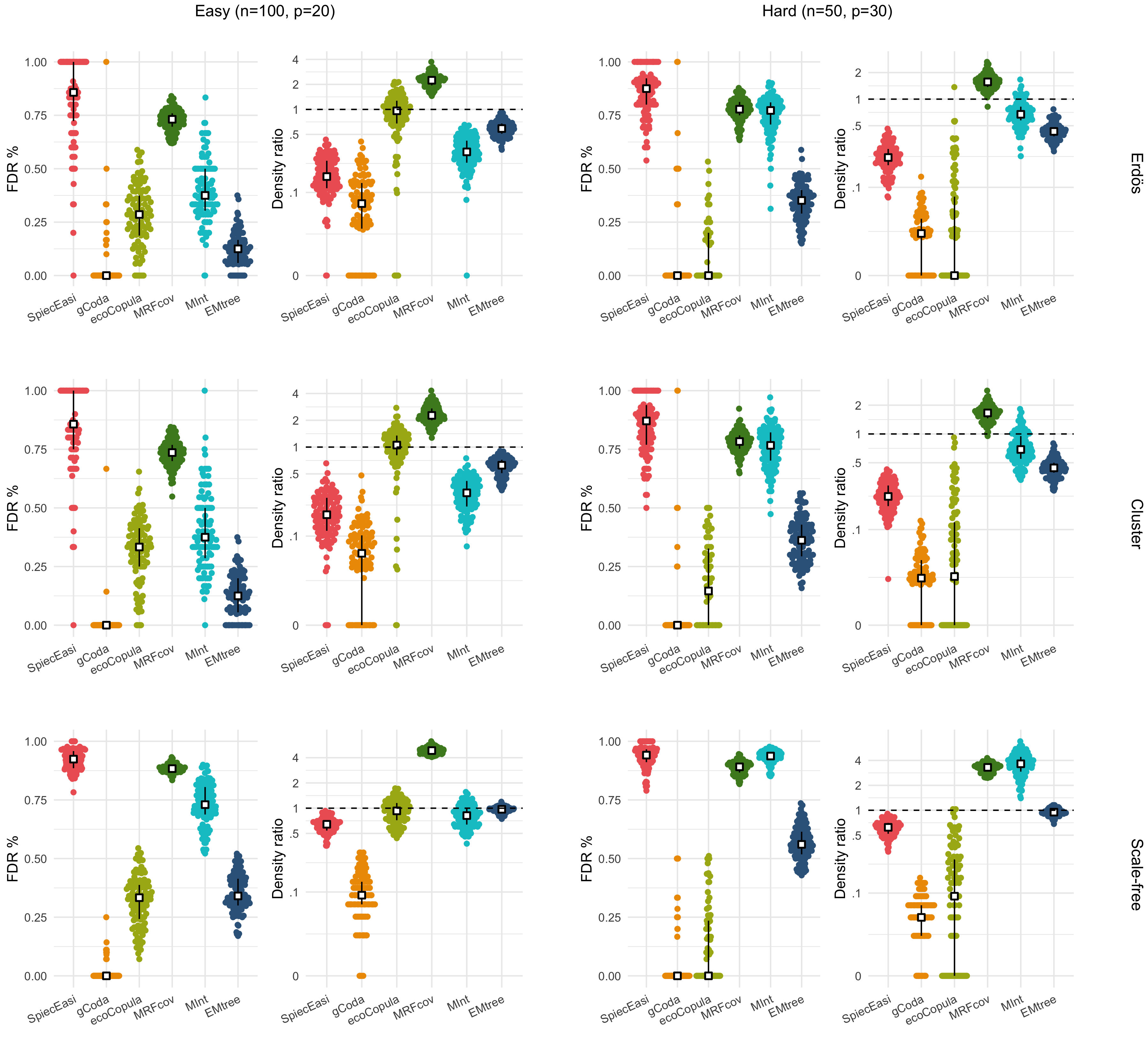
Figure 4: FDR and density ratio measures for all methods at two different difficulty levels and 100 networks of each type. White squares and black plain lines represent medians and quartiles respectively. ecoCopula selection method: AIC. Number of subsamples for SpiecEasi and EMtree: $S=20$. SpiecEasi and gCoda: $lambda.min.ratio=0.001$, $nlambda=100$.

	SpiecEasi	gCoda	ecoCopula	MRFcov	MInt	EMtree
Easy	25.45 (1.87)	0.11 (0.06)	5.55 (0.64)	34.51 (3.68)	43.04 (19.76)	11.72 (1.89)
Hard	28.43 (1.30)	0.53 (0.25)	9.6 (0.65)	8.29 (0.36)	33.77 (18.20)	8.17 (0.50)

Table 1: Median and standard-deviation running-time values (in seconds) for Cluster and Erdös structures, including resampling with $S=20$ for SpiecEasi and EMtree.

3.1.2 Effect of network structure

As expected for a fixed $p$, the higher the number of observations $n$, the better the performance for all methods and structures. Interestingly, the same happens when $p$ increases for a fixed $n=100$ (except for SpiecEasi). EMtree performs well on Scale-free structures (Fig. 5) which was also expected; the other methods performance worsen compared to other structures. When lowering $n$ to 30, EMtree performance deteriorates along with $p$, yet remaining above $70\%$ in median in the extreme case where $p=n$ (Fig. 5, right). The structure being Erdös or Cluster, each method is affected in the same way by an increase of $n$ or $p$ (Fig. 6). Besides, increasing the difference between the two structures by tuning up the ratio parameter has no effect. Overall EMtree performs better than gCoda and SpiecEasi on all the studied configurations. Running times are summarized in Table 2. EMtree is about 10 times slower than gCoda (4 for small $n$), and 4 times faster than SpiecEasi. The high standard deviation for small $n$ seems to be due to gCoda struggling with Scale-free structures.

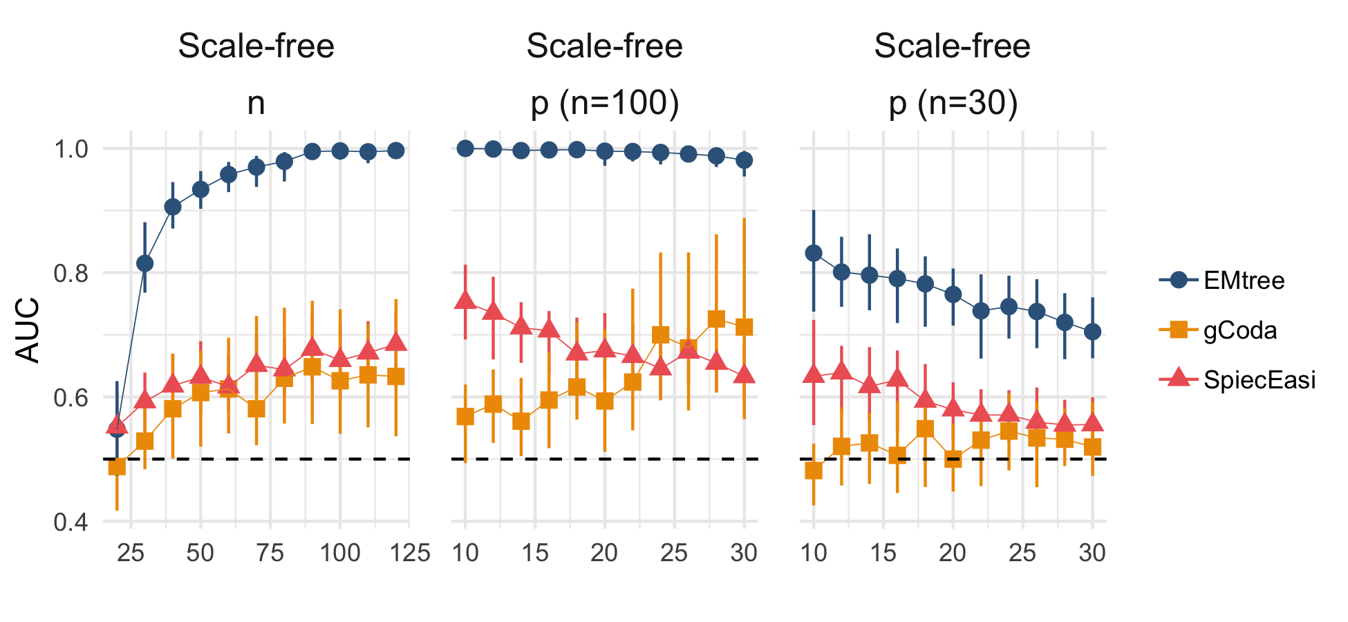
Figure 5: Effect of Scale-free structure on AUC medians and inter-quartile intervals for parameters $n$ and $p$.

	$n<50$	$n\geq 50$	$p<20$	$p\geq 20$
EMtree	0.44 (0.14)	0.60 (0.17)	0.41 (0.13)	0.76 (0.21)
gCoda	0.11 (26.8)	0.05 (0.05)	0.05 (0.04)	0.09 (0.54)
SpiecEasi	2.09 (0.26)	2.37 (0.28)	2.42 (0.27)	2.42 (0.26)

Table 2: Median and standard-deviation of running times for each method in seconds, for $n$ and $p$ parameters.

3.1.3 Effect of network density

The comparison of top and bottom panels of Fig. 6 shows that network inference gets harder as the network gets denser, whatever the method and the structure of the true graph. Running times are not affected (Table 8). Fig. 7 shows that EMtree performance does not deteriorate faster than that of other methods, demonstrating that the tree hypothesis is not a limitation.

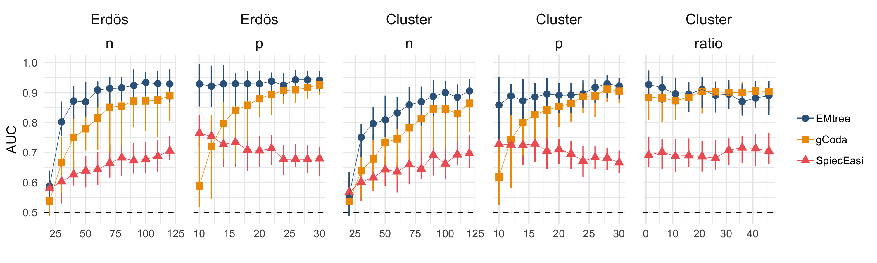
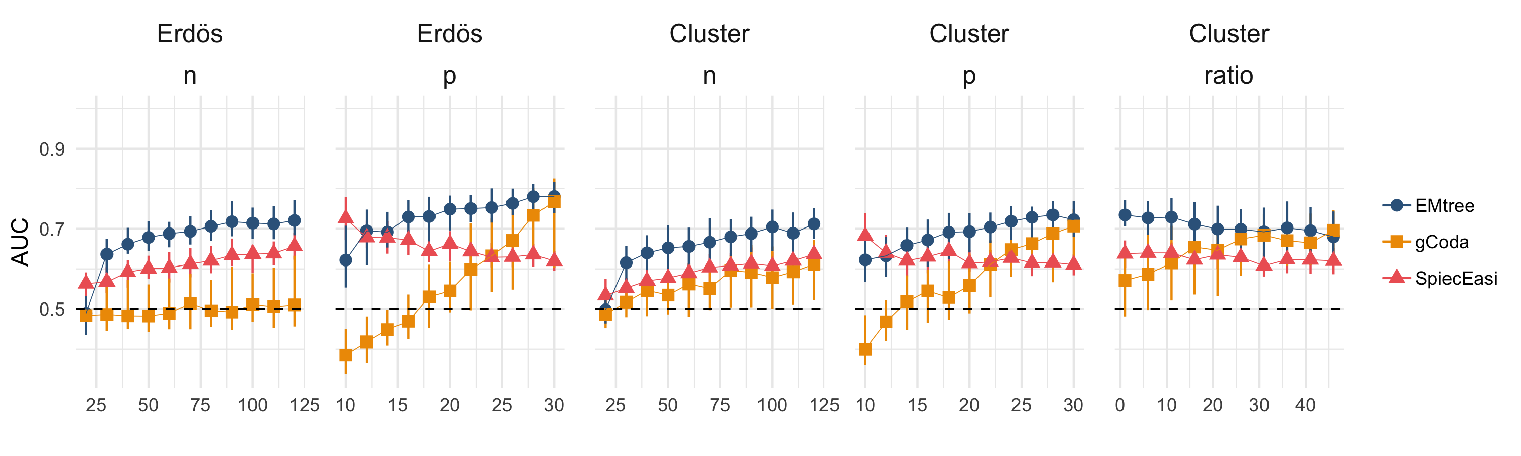
Figure 6: Effect of Erdös and Cluster structures on AUC medians and inter-quartile intervals for parameters $n$, $p$ and $ratio$. Top: densities set to $2/p$, bottom: densities set to $5/p$.

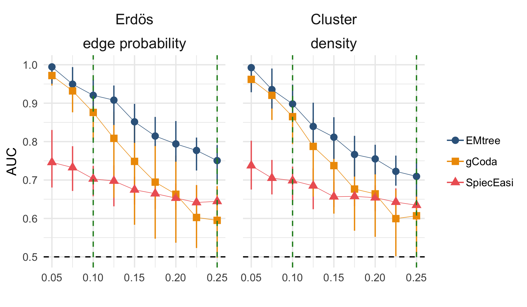
Figure 7: AUC median and inter-quartile intervals for parameters controlling the number of edges in Erdös (edge probability) and in Cluster (density) structures, $p=20$, $n=100$.

3.2 Illustrations

In this section we emphasize the importance of covariates for network inference. Accounting for environmental effects changes the structure of all inferred networks we present; nodes with the highest betweenness scores are highlighted to spot these changes. Most frequently, it results in reducing the number of edges (i.e. making the network sparser). However new edges can appear as well, as adjusting for a covariate also reduces the variability, which improves the detection power. In all examples, we used the resampling method described in Section 2.2, which provides edge selection frequencies. Eventually, we have to threshold these frequencies to draw actual networks; the value of the threshold obviously affects the density of the plotted networks (see Fig. 12).

3.2.1 Fish populations in the Fatala River estuary

Networks on Fig. 8 suggest a predominant role of the site covariate compared to the date. Indeed, adjusting for the site results in much sparser networks (Fig. 12 in appendix). It deeply modifies the network structure: the site network has 12 new edges and only 6 in common with the null network. Besides, the highlighted nodes only change when introducing the site covariate. This suggests that the environmental heterogeneity between the sites has a major effect on the variations of species abundances, while the effect of the date of sampling is moderate.

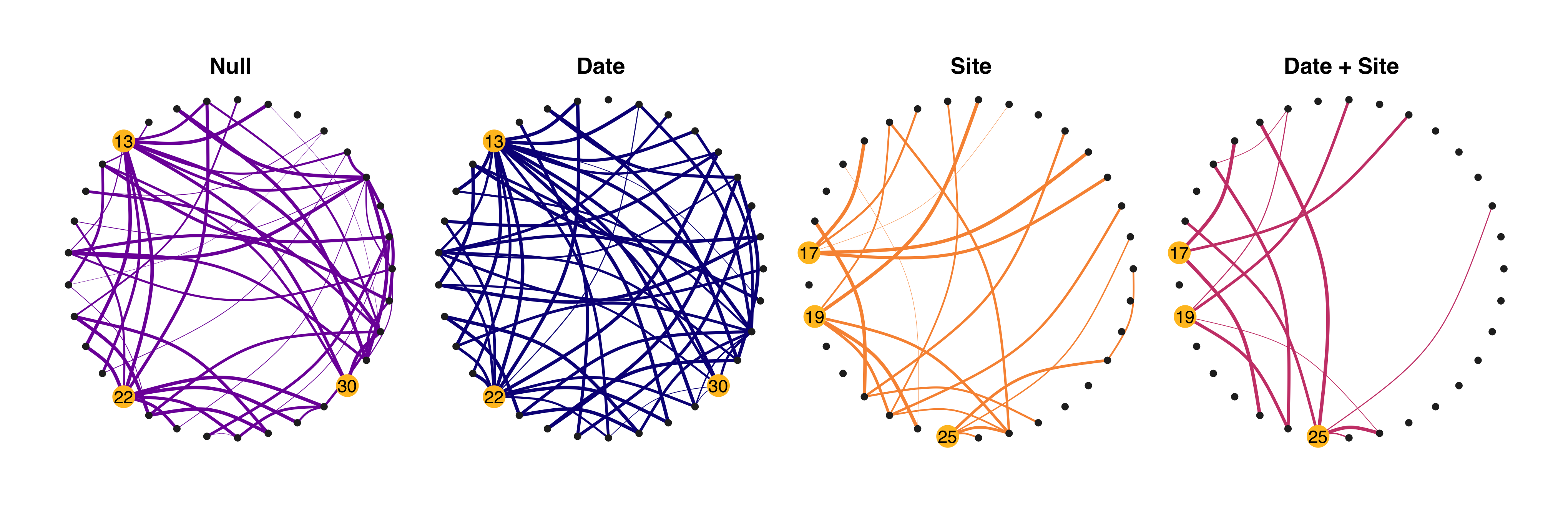
Figure 8: Interaction networks of Fatala River fishes inferred when adjusting for none, both or either one of the covariates among site and date. Highlighted nodes spot the highest betweenness centrality scores. Widths are proportional to selection frequencies. $S=100$, $f^{\prime}=90\%$.

3.2.2 Oak powdery mildew

When providing the inference with more information (tree status, distances), the structure of the resulting network is significantly modified. Nodes with high betweenness scores differ from one model to another. There is an important gap in density between the null model and the others, starting from a $25\%$ selection threshold (Fig. 12 in appendix). From a more biological point of view, the features of the pathogen node are greatly modified too: its betweenness score is among the smallest in the null network (quantile $16\%$), and among the highest in the two other networks (quantiles $93\%$ and $96\%$). Its connections to the other nodes vary as well. Accounting for covariates results in less interactions with the pathogen but a greater role of the latter in the pathobiome organization.

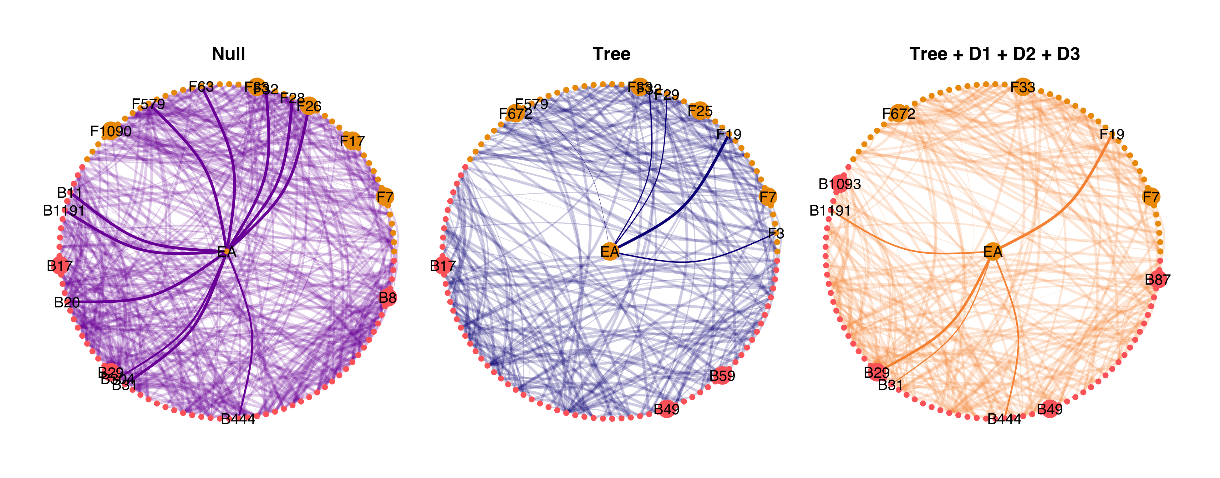
Figure 9: Pathogen interaction networks on oak leaves inferred with EMtree when adjusting for none, the tree covariate or tree and distances. Bigger nodes represent OTUs with highest betweenness values, colors differentiate fungal and bacterial OTUs. Widths are proportional to selection frequencies. $S=100$, $f^{\prime}=90\%$ .

Using the dataset restricted to infected samples (39 observations for 114 OTUs) and correcting for the leaves position in the tree (proxy for their abiotic environment), Jakuschkin et al. (2016) identifies a list of 26 OTUs likely to be directly interacting with the pathogen. Running EMtree on the same restricted dataset with the same correction yields a good concordance with edge selection frequencies, as shown in Fig. 10.

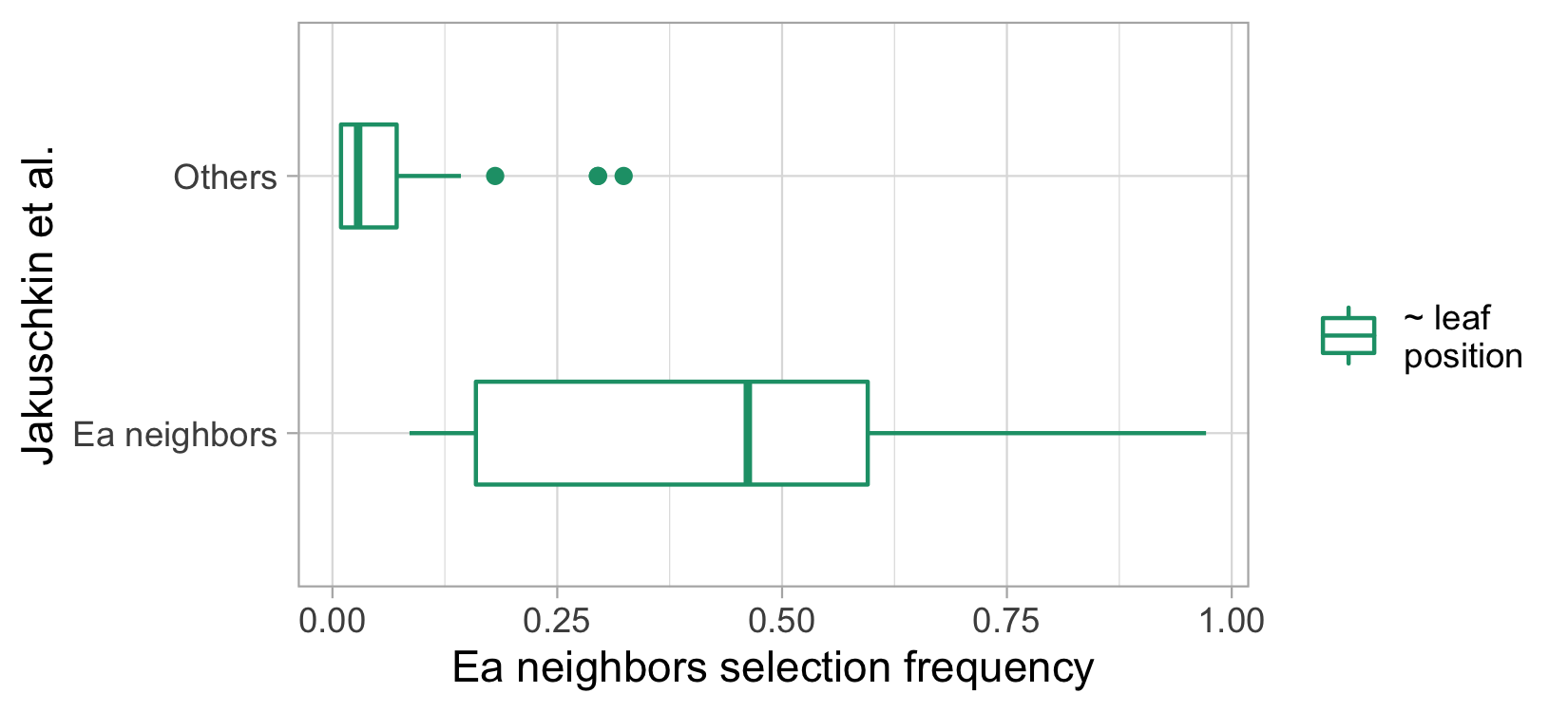
Figure 10: EMtree selection frequencies of pathogen neighbors compared to Jakuschkin et al. (2016) results, computed on infected samples and adjusting for the leaf position (100 subs-samples).

4 Discussion

The inference of species interaction network is a challenging task, for which a series of methods have been proposed in the past years. Abundance data seems to be a promising source of information for this purpose. Here we adopt the formalism of graphical models to define a probabilistic model-based framework for the inference of such networks from abundance data. Using a model-based approach offers several important advantages. First, it enables easy and explicit integration of environmental and experimental effects. These could be modeled in a more flexible way using generalized additive models, which include non-linear effects (Hastie, 2017). Then, as it also relies on a formal statistical definition of a species interaction network in the context of graphical models, accounting for abiotic effects and modeling species interactions are two clearly defined and distinguished goals. Finally, all the underlying assumptions are explicitly stated in the model definition itself, and can therefore be discussed and criticized.

We developed an efficient method to infer sparse networks, which combines a multivariate Poisson mixed model for the joint distribution of abundances, with an averaging over all spanning trees to efficiently infer direct species interactions. As we do consider a mixture over all spanning trees, our approach remains flexible and can infer most types of statistical dependencies. An EM algorithm (EMtree) maximizes the likelihood of the result and returns each edge probability to be part of the network. An optional resampling step increases network robustness.

A simulation study in a heterogeneous environment demonstrates that EMtree compares very well to alternative approaches. The proposed model can take all kind of covariates into account, which when ignored can have dramatic effects on the inferred network structure, as showed here on empirical datasets. Experiments on simulated data and illustrations also demonstrate that EMtree computational cost remains very reasonable.

Alternative methods used in this work all rely on an optimized threshold to tell an edge presence. This particular threshold is obtained after testing a grid of possible values which all yield a different network, and altogether build a path. Making this path available to the user is useful, as the final threshold might need modification and it gives the possibility to build edges scores and get more than a binary result. We found few recent approaches doing this, which prevented us to study their performance in a way that did not impose a threshold.

The proposed methodology could be extended in several ways. Species abundances and interactions indeed vary across space, and depend on local conditions (Poisot et al., 2012, 2015). This can either be considered as nuisance parameter or as feature of interest. In the first case, the method could be extended to account for the spatial autocorrelation of sampling sites, to obtain a ”regional” interaction network corrected for this effect, i.e. assuming the network is the same in all sites. If of interest, variation across space and local conditions could be studied by comparing networks inferred from the different sampling locations. Networks comparison is a wide and interesting question and tools lack to check which edges are shared by a set of networks. The approach introduced by Schwaller and Robin (2017) could be adapted to EMtree framework. Lastly, It is also very likely that not all covariates nor even all species have been measured or observed. Another extension may therefore be to detect ignored covariates or missing species. To this purpose EMtree could probably be combined with the approach developed by Robin et al. (2018) to identify missing actors.

Data accessibility.

The method developed in this paper is implemented in the R package EMtree available on GitHub: https://github.com/Rmomal/EMtree.

Acknowledgement.

The authors thank P. Gloaguen and M. Authier for helpful discussions and C. Vacher for providing the oak data set. This work is partly funded by ANR-17-CE32-0011 NGB and by a public grant as part of the Investissement d’avenir project, reference ANR-11-LABX-0056-LMH, LabEx LMH.

Author’s contributions statement.

All authors conceived the ideas and designed methodology; R. Momal developed and tested the algorithm. All authors led the writing of the manuscript, contributed critically to the drafts and gave final approval for publication.

Annex A Supplement: Methods

A.1 Variational EM in the observed layer

A reminder on EM and VEM.

Expectation-Maximisation (EM: Dempster et al., 1977) has become the standard algorithm for the maximum likelihood inference of latent variable models. Denoting ${\bm{\gamma}}$ the unknown parameter, ${\bf Y}$ the observed variables and ${\bf H}$ the latent variables, the aim of EM is to maximise the observed (log-)likelihood $\log p_{\bm{\gamma}}({\bf Y})$. In the model defined in Section 2.1, the set of parameter to estimate is ${\bm{\gamma}}=({\bm{\beta}},{\bm{\Sigma}},{\bm{\theta}})$ and the latent variables are ${\bf H}=({\bf Z},T)$. Because the complete (log-)likelihood $\log p_{\bm{\gamma}}({\bf Y},{\bf H})$ is often much easier to handle, EM alternatively evaluates the conditional distribution of the latent variables $p_{\bm{\gamma}}({\bf H}\mid{\bf Y})$ (E step) and updates the parameter estimates by maximizing the conditional expectation of the complete log-likelihood (M step).

Unfortunately, for many models, the conditional distribution $p_{\bm{\gamma}}({\bf H}\mid{\bf Y})$ is intractable. The variational EM (VEM) algorithm has been designed to deal with such cases. Briefly speaking, the E step (during which the intractable conditional distribution should be evaluated) is replaced with a VE step, during which an approximate distribution $\widetilde{p}({\bf Y})\simeq p_{\bm{\gamma}}({\bf H}\mid{\bf Y})$ is determined. Actually, the VEM algorithm maximizes a lower bound of the genuine log-likelihood, similar to this given in Eq. (6) (see Ormerod and Wand, 2010; Blei et al., 2017, for an introduction).

Application to the Poisson log-normal model.

To estimate the fixed regression parameters gathered in ${\bm{\theta}}$, we resort to a surrogate model where the entries of the abundance matrix ${\bf Y}$ still have the conditional distribution given in Eq. (1), but where the distribution of the ${\bf Z}_{i}$ is not constrained to be faithful to a specific graphical model. Namely, the latent vectors ${\bf Z}_{i}$ are only supposed to be independent and identically distributed (iid) Gaussian with distribution $\mathcal{N}(0,{\bm{\Sigma}})$, without any restriction on ${\bm{\Sigma}}$.

This surrogate model is actually a Poisson log-normal model as introduced by Aitchison and Ho (1989), the parameters of which can be estimated using a variational approximation similar to this introduced in Chiquet et al. (2018). More specifically, we maximize with respect to the parameters ${\bm{\theta}}$ and ${\bm{\Sigma}}$ the following lower bound of the log-likelihood $\log p({\bf Y})$:

$$\mathcal{J}({\bf Y};{\bm{\theta}},{\bm{\Sigma}},\widetilde{p}):=\log p_{{\bm{\theta}},{\bm{\Sigma}}}({\bf Y})-KL\left(\widetilde{p}({\bf Z})||p_{{\bm{\theta}},{\bm{\Sigma}}}({\bf Z}\mid{\bf Y})\right),$$ (6)

where $KL(q||p)$ stands for Küllback-Leibler divergence between distributions $q$ and $p$ and where the approximate distribution $\widetilde{p}({\bf Z})$ is chosen to be Gaussian. This means that each conditional distribution $p({\bf Z}_{i}\mid{\bf Y}_{i})$ is approximated with a normal distribution $\mathcal{N}(\widetilde{\bf m}_{i},\widetilde{\bf S}_{i})$. As shown in Chiquet et al. (2018), $\mathcal{J}({\bf Y},{\bm{\theta}},{\bm{\Sigma}},\widetilde{p})$ is bi-concave in $({\bm{\theta}},{\bm{\Sigma}})$ and $\{(\widetilde{\bf m}_{i},\widetilde{\bf S}_{i})_{i}\}$, so that gradient ascent can be used. The PLNmodels R-package –available on GitHub– provides an efficient implementation of it.

The entries of the $\widetilde{\bf m}_{i}$ and $\widetilde{\bf S}_{i}$ provide us with approximations of the conditional expectation, variance and covariance of the $Z_{ij}$ conditionally on the ${\bf Y}$, which we use to get the estimates $\widehat{\sigma}_{j}^{2}$ and $\widehat{\rho}_{jk}$ given in Eq. (8). More specifically, we use $\operatorname*{\mathbb{E}}(Z_{ij}\mid{\bf Y}_{i})\simeq\widetilde{m}_{ij}$, $\operatorname*{\mathbb{E}}(Z^{2}_{ij}\mid{\bf Y}_{i})\simeq\widetilde{m}_{ij}^{2}+\widetilde{S}_{i,jj}$ and $\operatorname*{\mathbb{E}}(Z_{ij}Z_{ik}\mid{\bf Y}_{i})\simeq\widetilde{m}_{ij}\widetilde{m}_{ik}+\widetilde{S}_{i,jk}$.

A.2 EM in the latent layer

Complete log-likelihood conditional expectation

Because of the specific form given in Eq. (3), and because the ${\bf Z}_{i}\mid T$ are Gaussian, we have that

$$\log{p_{\bm{\Sigma}}}({\bf Z}\mid T) =\sum_{j=1}^{p}\sum_{i=1}^{n}\log P(Z_{ij}\mid T)+\sum_{(j,k)\in T}\sum_{i=1}^{n}\log\left(\frac{P(Z_{ij},Z_{ik})}{P(Z_{ij})P(Z_{ik})}\right)$$

$$=-\frac{n}{2}\log\sigma_{j}^{2}-\frac{1}{2}\sum_{j=1}^{p}\sum_{i=1}^{n}\frac{Z_{ij}^{2}}{\sigma_{j}^{2}}-\frac{n}{2}\sum_{(j,k)\in T}\log(1-\rho_{jk}^{2})$$ (7)

$$\quad-\frac{1}{2}\sum_{(j,k)\in T}\frac{1}{1-\rho_{jk}^{2}}\sum_{i=1}^{n}\left(\rho^{2}_{jk}\frac{Z_{ij}^{2}}{\sigma_{j}^{2}}+\rho^{2}_{jk}\frac{Z_{ik}^{2}}{\sigma_{k}^{2}}-2\rho_{jk}\frac{Z_{ij}Z_{ik}}{\sigma_{j}\sigma_{k}}\right)+\text{cst}$$

where the constant term does not depend on any unknown parameter. In the EM algorithm, we have to maximize the conditional expectation of Eq. (A.2) with respect to the variances $\sigma_{j}^{2}$ and the correlation coefficients $\rho_{jk}$. The resulting estimates take the usual forms, but with the conditional moments of the $Z_{ij}$, that is

$$\widehat{\sigma}_{j}^{2}=\frac{1}{n}\sum_{i}\operatorname*{\mathbb{E}}(Z^{2}_{ij}\mid{\bf Y}),\qquad\widehat{\rho}_{jk}=\frac{1}{n}\sum_{i}\operatorname*{\mathbb{E}}(Z_{ij}Z_{ik}\mid{\bf Y})\left/(\widehat{\sigma}_{j}\widehat{\sigma}_{k})\right..$$ (8)

which do not depend on T. The maximized conditional expectation of Eq. (A.2) becomes

$$\operatorname*{\mathbb{E}}\left(\log p_{\widehat{{\bm{\Sigma}}}}({\bf Z}\mid T)\mid{\bf Y}\right)=-\frac{n}{2}\log\widehat{\sigma}_{j}^{2}-\frac{n}{2}\sum_{(j,k)\in T}\log(1-\widehat{\rho}_{jk}^{2})+\text{cst}.$$ (9)

We are left with the writing of the conditional expectation of the first two terms of the logarithm of Eq. (4), once optimized in ${\bm{\Sigma}}$. Combining Eq. (2) and Eq. (9), and noticing that the probability for an edge to be part of the graph is the sum of the probability of all the trees than contain this edge, we get (denoting $\log\widehat{\psi}_{jk}=(1-\widehat{\rho}_{jk}^{2})^{-n/2}$)

$$\operatorname*{\mathbb{E}}\left(\log p_{\bm{\beta}}(T)+\log p_{\widehat{{\bm{\Sigma}}}}({\bf Z}\mid T)\mid{\bf Y}\right) =\sum_{T\in\mathcal{T}}p(T\mid{\bf Y})\left(\log p_{\bm{\beta}}(T)+\log p_{\widehat{{\bm{\Sigma}}}}({\bf Z}\mid T)\right)$$

$$=-\log B+\sum_{T\in\mathcal{T}}p(T\mid{\bf Y})\sum_{(j,k)\in T}\left(\log\beta_{jk}+\log\widehat{\psi}_{jk}\right)+\text{cst}$$

$$=-\log B+\sum_{(j,k)}\operatorname*{\mathds{P}}\{(j,k)\in T\mid{\bf Y}\}\left(\log\beta_{jk}+\log\widehat{\psi}_{jk}\right)+\text{cst},$$

which gives Eq. (5).

As explained in the section above, we approximate expectations and probabilities conditional on ${\bf Y}$ by their variational approximation. This provides us with the approximate conditional distribution of the tree $T$ given the data ${\bf Y}$: ~p(T ∣Y) = ∏_jk ∈T β_jk ^ψ_jk / C, where $C$ is the normalizing constant: $C=\sum_{T}\prod_{j,k\in T}\beta_{jk}\widehat{\psi}_{jk}$. The intuition behind this approximation is the following: according to Eq. (2), the marginal probability a tree $T$ is proportional to the product of the weights $\beta_{jk}$ of its edges. The conditional distribution probability of tree is proportional to the same product, the weights $\beta_{jk}$ being updated as $\beta_{jk}\widehat{\psi}_{jk}$, where $\widehat{\psi}_{jk}$ summarizes the information brought by the data about the edge ($j,k$).

Steps E and M

E step:

From the above computation we get the following approximation:

P({j,k}∈T ∣Y) ≃1 - ∑_T:jk∉T ~p(T ∣Y), and so we define $p_{jk}$ as follows: P_jk= 1 - ∑T:jk∉T∏j, k ∈Tβjkψjk∑T∏j, k ∈Tβjkψjk. $P_{jk}$ can be computed with Theorem 1, letting $[{\bf W}^{h}]_{jk}=\beta^{h}_{jk}\widehat{\psi}_{jk}$ and ${\bf W}^{h}_{\setminus{jk}}={\bf W}^{h}$ except for the entries $(j,k)$ and $(k,j)$ which are set to 0. The modification of ${\bf W}^{h}_{\setminus{jk}}$ with respect to ${\bf W}^{h}$ amounts to set to zero the weight product, and so the probability, for any tree $T$ containing the edge $(j,k)$. As a consequence, we get P^h+1_jk= 1 - —Q_uv^*(W^h_∖jk)— / —Q_uv^*(W^h)— .

M step:

Applying Lemma 1 to the weight matrix ${\bm{\beta}}$, the derivative of $B$ with respect to $\beta_{jk}$ is ∂_β_jk B = [M(β)]_jk×B then the derivative of (5) with respect to $\beta_{jk}$ is null for $\beta^{h+1}_{jk}=P_{jk}^{h+1}\left/[{\bf M}({\bm{\beta}}^{h})]_{jk}\right.$.

A.3 Matrix tree theorem

For any matrix ${\bf W}$, we denote its entry in row $u$ and column $v$ by $[{\bf W}]_{uv}$. We define the Laplacian matrix ${\bf Q}$ of a symmetric matrix ${\bf W}=[w_{jk}]_{1\leq j,k\leq p}$ as follows :

$$[{\bf Q}]_{jk}=\begin{cases}-w_{jk}&1\leq j<k\leq p\\ \sum_{u=1}^{p}w_{ju}&1\leq j=k\leq p.\end{cases}$$

We further denote ${\bf W}^{uv}$ the matrix ${\bf W}$ deprived from its $u$th row and $v$th column and we remind that the $(u,v)$-minor of ${\bf W}$ is the determinant of this deprived matrix, that is $|{\bf W}^{uv}|$.

Theorem 1 (Matrix Tree Theorem Chaiken and Kleitman (1978); Meilă and Jaakkola (2006)).

For any symmetric weight matrix W, the sum over all spanning trees of the product of the weights of their edges is equal to any minor of its Laplacian. That is, for any $1\leq u,v\leq p$,

$$W:=\sum_{T\in\mathcal{T}}\prod_{(j,k)\in T}w_{jk}=|{\bf Q}^{uv}|.$$

In the following, without loss of generality, we will choose ${\bf Q}^{pp}$. As an extension of this result, Meilă and Jaakkola (2006) provide a close form expression for the derivative of $W$ with respect to each entry of ${\bf W}$.

Lemma 1 (Meilă and Jaakkola (2006)).

Define the entries of the symmetric matrix ${\bf M}$ as

$$[{\bf M}]_{jk}=\begin{cases}\left[({\bf Q}^{pp})^{-1}\right]_{jj}+\left[({\bf Q}^{pp})^{-1}\right]_{kk}-2\left[({\bf Q}^{pp})^{-1}\right]_{jk}&1\leq j<k<p\\ \left[({\bf Q}^{pp})^{-1}\right]_{jj}&k=p,1\leq j\leq p\\ 0&1\leq j=k\leq p.\end{cases}$$

it holds that ∂_w_jk W = [M]_jk×W.

Annex B Supplement

B.1 Simulation results

B.1.1 Effect of dataset dimensions

		SpiecEasi	gCoda	ecoCopula	MRFcov	MInt	EMtree
Easy	Cluster	0.86 (0.20)	0 (0.08)	0.33 (0.14)	0.74 (0.06)	0.38 (0.17)	0.12 (0.09)
	Erdös	0.86 (0.21)	0 (0.15)	0.29 (0.15)	0.73 (0.05)	0.38 (0.15)	0.12 (0.08)
	Scale-free	0.92 (0.04)	0 (0.04)	0.33 (0.11)	0.88 (0.02)	0.73 (0.09)	0.34 (0.08)
Hard	Cluster	0.87 (0.12)	0 (0.20)	0.15 (0.18)	0.78 (0.05)	0.77 (0.09)	0.36 (0.09)
	Erdös.	0.88 (0.11)	0 (0.24)	0 (0.15)	0.78 (0.05)	0.77 (0.10)	0.35 (0.09)
	Scale-free	0.94 (0.05)	0 (0.13)	0 (0.16)	0.89 (0.03)	0.94 (0.03)	0.56 (0.07)

Table 3: Medians and standard-deviation of FDR computed on 100 graphs of each type (easy: $n=100,p=20$, hard: $n=50,p=30$)

		SpiecEasi	gCoda	ecoCopula	MRFcov	MInt	EMtree
Easy	Cluster	0.16 (0.11)	0.05 (0.07)	1.04 (0.48)	2.26 (0.58)	0.30 (0.13)	0.62 (0.14)
	Erdös	0.15 (0.09)	0.06 (0.08)	0.95 (0.50)	2.23 (0.42)	0.30 (0.14)	0.58 (0.12)
	Scale-free	0.63 (0.13)	0.08 (0.07)	0.92 (0.30)	4.86 (0.44)	0.81 (0.25)	0.96 (0.08)
Hard	Cluster	0.21 (0.08)	0.02 (0.03)	0.02 (0.17)	1.65 (0.33)	0.68 (0.30)	0.43 (0.10)
	Erdös	0.21 (0.08)	0.02 (0.02)	0.00 (0.18)	1.56 (0.32)	0.66 (0.25)	0.42 (0.10)
	Scale-free	0.61 (0.12)	0.04 (0.03)	0.08 (0.24)	3.29 (0.40)	3.63 (1.08)	0.94 (0.09)

Table 4: Medians and standard-deviation of density ratio computed on 100 graphs of each type (easy: $n=100,p=20$, hard: $n=50,p=30$)

		SpiecEasi	gCoda	ecoCopula	MRFcov	MInt	EMtree
Easy	Cluster	1.77	13.89	1.74	0.00	0.00	0.00
	Erdös	0.68	11.95	0.99	0.00	0.83	0.00
	Scale-free	0.00	1.88	0.00	0.00	0.00	0.00
Hard	Cluster	0.00	14.05	23.40	0.00	0.00	0.00
	Erdös	0.00	20.85	27.28	0.00	0.00	0.00
	Scale-free	0.00	5.97	15.46	0.00	0.00	0.00

Table 5: Percentage of empty networks computed on 100 graphs of each type (easy: $n=100,p=20$, hard: $n=50,p=30$)

	SpiecEasi	gCoda	ecoCopula	MRFcov	MInt	EMtree
Easy	29.73 (2.00)	1.29 ( 0.30)	28.14 (1.46)	48.7 (2.32)	138.13 (39.60)	50.19 (7.81)
Hard	29.38 (1.31)	40.73 (20.94)	27.16 (1.30)	14.1 (0.36)	95.27 (46.34)	23.59 (2.09)

Table 6: Median and standard-deviation of running times in seconds for scale-free structures, for two dataset dimensions (easy: $n=100$, $p=20$, hard: $n=50$, $p=30$).

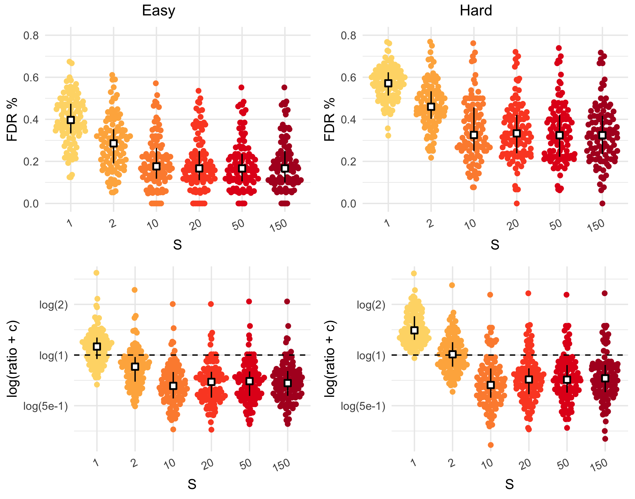
Figure 11: FDR and density ratio measures of EMtree with varying values of number of sub-samples $S$ (Erdös structure).

$S$	1	2	10	20	50	150
Easy	0.66 (0.15)	1.86 (0.23)	7.00 (0.81)	12.29 (1.27)	29.50 (3.39)	87.30 (10.36)
Hard	0.45 (0.12)	1.44 (0.14)	5.06 (0.78)	8.97 (0.87)	23.35 (2.40)	69.29 (10.83)

Table 7: Median and standard-deviation running-time values in seconds for inference of Erdös structure with EMtree and different values of the number of sub-samples $S$.

B.1.2 Effect of network density

	$n<50$	$n\geq 50$	$p<20$	$p\geq 20$
EMtree	0.41 (0.11)	0.60 (0.15)	0.38 (0.12)	0.71 (0.21)
gCoda	0.12 (0.47)	0.07 (0.03)	0.05 (0.03)	0.09 (0.06)
SpiecEasi	2.41 (0.25)	2.41 (0.25)	2.39 (0.25)	2.42 (0.25)

Table 8: Median and standard-deviation of running times for each method in seconds, for $n$ and $p$ parameters. corresponding to Erdös and cluster structures with $5/p$ densities.

B.2 Illustrations

B.2.1 Effect of the edge frequency threshold

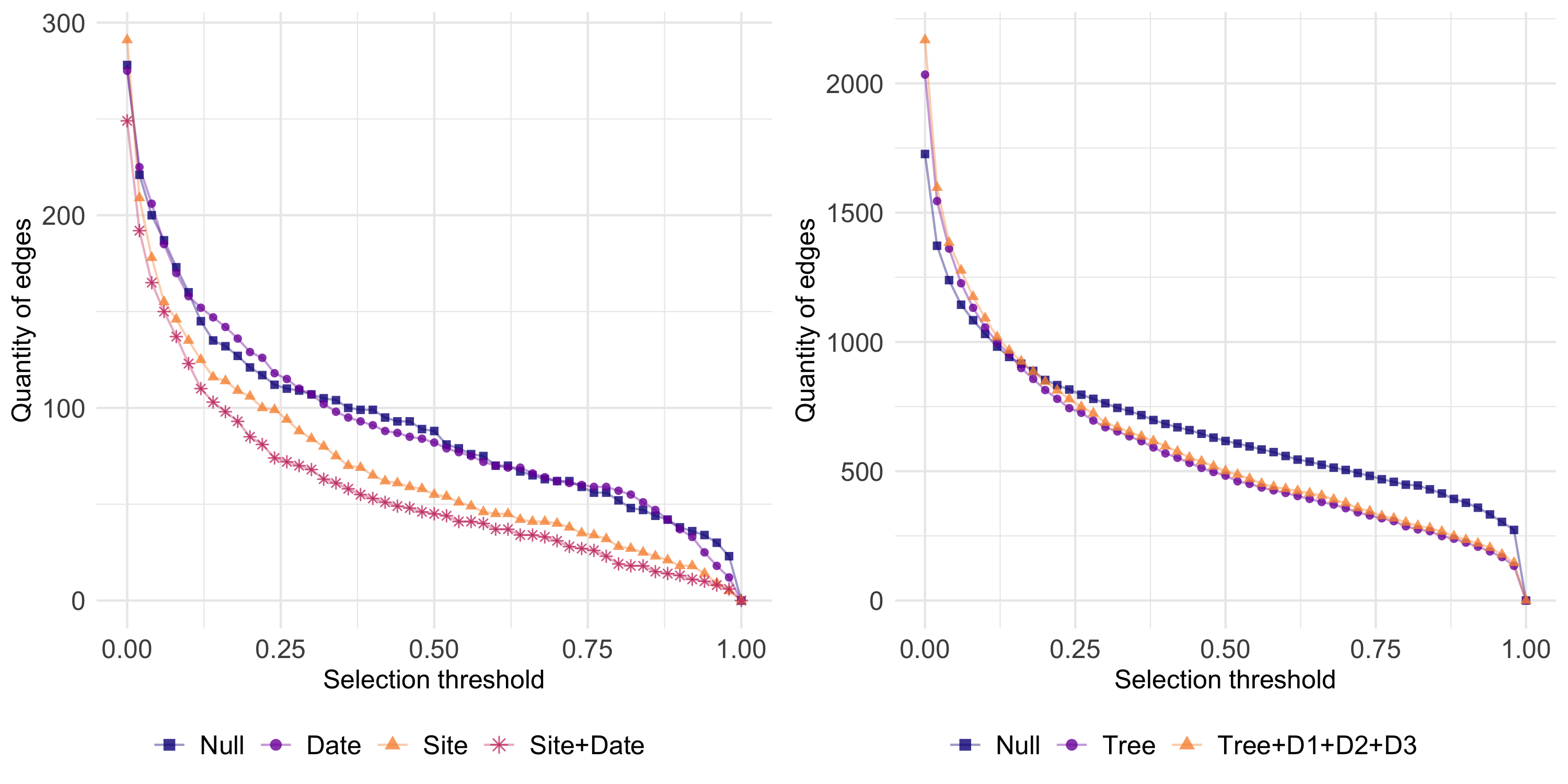
Figure 12: Quantity of selected edges as a function of the selection threshold (left: Fatala fishes, right: oak mildew.)

The curves displayed on Fig. 12 are very smooth, which illustrates the difficulty of setting this threshold.

B.2.2 Fatala River fishes

Species names with highest betweenness scores:

13: Galeoides decadactylus, 17:Ilisha africana,19: Liza grandisquamis, 22: Pseudotolithus brachygnatus, 25: Pellonula leonensis, 30: Pseudotolithus typus.

References

- Valiente-Banuet et al. (2015) A. Valiente-Banuet, M. A. Aizen, J. M. Alcántara, J. Arroyo, A. Cocucci, M. Galetti, M. B. García, D. García, J. M. Gómez, P. Jordano, et al., Functional Ecology 29, 299 (2015).
- Jordano (2016) P. Jordano, Functional Ecology 30, 1883 (2016).
- Poisot et al. (2016) T. Poisot, D. B. Stouffer, and S. Kéfi, Functional Ecology 30, 1878 (2016).
- Faust and Raes (2012) K. Faust and J. Raes, Nature Reviews Microbiology 10, 538 (2012).
- Evans et al. (2016) D. M. Evans, J. J. Kitson, D. H. Lunt, N. A. Straw, and M. J. Pocock, Functional ecology 30, 1904 (2016).
- Olito and Fox (2015) C. Olito and J. W. Fox, Oikos 124, 428 (2015).
- Bartomeus et al. (2016) I. Bartomeus, D. Gravel, J. M. Tylianakis, M. A. Aizen, I. A. Dickie, and M. Bernard-Verdier, Functional Ecology 30, 1894 (2016).
- Weinstein and Graham (2017) B. G. Weinstein and C. H. Graham, Ecology letters 20, 326 (2017).
- Graham and Weinstein (2018) C. H. Graham and B. G. Weinstein, Ecology letters 21, 1299 (2018).
- Wells and O’Hara (2013) K. Wells and R. B. O’Hara, Methods in Ecology and Evolution 4, 1 (2013).
- Desjardins-Proulx et al. (2017) P. Desjardins-Proulx, I. Laigle, T. Poisot, and D. Gravel, PeerJ 5, e3644 (2017).
- Stock et al. (2017) M. Stock, T. Poisot, W. Waegeman, and B. De Baets, Scientific reports 7, 45908 (2017).
- Dallas et al. (2017) T. Dallas, A. W. Park, and J. M. Drake, PLoS computational biology 13, e1005557 (2017).
- Friedman (2004) N. Friedman, Science 303, 799 (2004).
- Zhu and Cribben (2018) Y. Zhu and I. Cribben, Brain connectivity 8, 139 (2018).
- Popovic et al. (2019) G. C. Popovic, D. I. Warton, F. J. Thomson, F. K. C. Hui, and A. T. Moles, Methods in Ecology and Evolution 10, 1571 (2019).
- Elith and Leathwick (2009) J. Elith and J. R. Leathwick, Annual review of ecology, evolution, and systematics 40 (2009).
- Harris (2015) D. J. Harris, Methods in Ecology and Evolution 6, 465 (2015).
- Ovaskainen et al. (2017) O. Ovaskainen, G. Tikhonov, A. Norberg, F. Guillaume B., L. Duan, D. Dunson, T. Roslin, and N. Abrego, Ecology Letters 20, 561 (2017).
- Popovic et al. (2018) G. C. Popovic, F. K. Hui, and D. I. Warton, Journal of Multivariate Analysis 165, 86 (2018).
- Warton et al. (2015) D. I. Warton, F. G. Blanchet, R. B. O’Hara, O. Ovaskainen, S. Taskinen, S. C. Walker, and F. K. Hui, Trends in Ecology & Evolution 30, 766 (2015).
- Aitchison and Ho (1989) J. Aitchison and C. Ho, Biometrika 76, 643 (1989).
- Dormann et al. (2018) C. F. Dormann, M. Bobrowski, D. M. Dehling, D. J. Harris, F. Hartig, H. Lischke, M. D. Moretti, J. Pagel, S. Pinkert, M. Schleuning, et al., Global ecology and biogeography 27, 1004 (2018).
- Lauritzen (1996) S. L. Lauritzen, Graphical Models, Oxford Statistical Science Series (Clarendon Press, 1996).
- Clark et al. (2018) N. J. Clark, K. Wells, and O. Lindberg, Ecology 99, 1277 (2018).
- Morueta-Holme et al. (2016) N. Morueta-Holme, B. Blonder, B. Sandel, B. J. McGill, R. K. Peet, J. E. Ott, C. Violle, B. J. Enquist, P. M. Jørgensen, and J.-C. Svenning, Ecography 39, 1139 (2016).
- Friedman et al. (2008a) J. Friedman, T. Hastie, and R. Tibshirani, Biostatistics 9, 432 (2008a).
- Chow and Liu (1968) C. Chow and C. Liu, IEEE Transactions on Information Theory 14, 462 (1968).
- Meilă and Jaakkola (2006) M. Meilă and T. Jaakkola, Statistics and Computing 16, 77 (2006).
- Kirshner (2008) S. Kirshner, in Advances in Neural Information Processing Systems (2008), pp. 761–768.
- Ovaskainen et al. (2010) O. Ovaskainen, J. Hottola, and J. Siitonen, Ecology 91, 2514 (2010).
- Ulrich and Gotelli (2010) W. Ulrich and N. J. Gotelli, Ecology 91, 3384 (2010).
- Biswas et al. (2016) S. Biswas, M. McDonald, D. S. Lundberg, J. L. Dangl, and V. Jojic, Journal of Computational Biology 23, 526 (2016).
- Austin (2007) M. Austin, Ecological modelling 200, 1 (2007).
- Richards (2008) S. A. Richards, Journal of Applied Ecology 45, 218 (2008).
- Schwaller et al. (2019) L. Schwaller, S. Robin, and M. Stumpf, J. Soc. Franc. Stat. 160, 1 (2019).
- Dempster et al. (1977) A. P. Dempster, N. M. Laird, and D. B. Rubin, J. Royal Statist. Soc., series B 39, 1 (1977).
- Chaiken and Kleitman (1978) S. Chaiken and D. J. Kleitman, Journal of combinatorial theory, Series A 24, 377 (1978).
- Liu et al. (2010) H. Liu, K. Roeder, and L. Wasserman (Curran Associates Inc., USA, 2010), NIPS’10, pp. 1432–1440.
- Kurtz et al. (2015) Z. D. Kurtz, C. L. Müller, E. R. Miraldi, D. R. Littman, M. J. Blaser, and R. A. Bonneau, PLoS computational biology 11, e1004226 (2015).
- Fang et al. (2017) H. Fang, C. Huang, H. Zhao, and M. Deng, Journal of Computational Biology 24, 699 (2017).
- Friedman et al. (2008b) J. Friedman, T. Hastie, and R. Tibshirani, Biostatistics 9, 432 (2008b).
- Zhao et al. (2012) T. Zhao, H. Liu, K. Roeder, J. Lafferty, and L. Wasserman, Journal of Machine Learning Research 13, 1059 (2012).
- Baran (1995) E. Baran, Ph.D. thesis, Thèse de Doctorat, Université de Bretagne Occidentale (1995).
- Jakuschkin et al. (2016) B. Jakuschkin, V. Fievet, L. Schwaller, T. Fort, C. Robin, and C. Vacher, Microb Ecol 72, 870 (2016).
- Freeman (1978) L. C. Freeman, Social networks 1, 215 (1978).
- Hastie (2017) T. J. Hastie, in Statistical models in S (Routledge, 2017), pp. 249–307.
- Poisot et al. (2012) T. Poisot, E. Canard, D. Mouillot, N. Mouquet, and D. Gravel, Ecology letters 15, 1353 (2012).
- Poisot et al. (2015) T. Poisot, D. B. Stouffer, and D. Gravel, Oikos 124, 243 (2015).
- Schwaller and Robin (2017) L. Schwaller and S. Robin, Statistics and Computing 27, 1331 (2017).
- Robin et al. (2018) G. Robin, C. Ambroise, and S. Robin, Statistical Modelling p. 1471082X18786289 (2018).
- Ormerod and Wand (2010) J. T. Ormerod and M. P. Wand, The American Statistician 64, 140 (2010).
- Blei et al. (2017) D. M. Blei, A. Kucukelbir, and J. D. McAuliffe, Journal of the American Statistical Association 112, 859 (2017).
- Chiquet et al. (2018) J. Chiquet, M. Mariadassou, and S. Robin, The Annals of Applied Statistics 12, 2674 (2018).