Solar Center–Limb Variation of the Strengths of Spectral Lines: Classification and Interpretation of Observed Trends

Abstract

The equivalent widths ($W$) of 565 spectral lines in the wavelength range of 4690–6870 Å were evaluated at 31 consecutive points from the solar disk center ($\mu\equiv\cos\theta=1$) to near the limb ($\mu=0.25$) by applying the synthetic spectrum-fitting technique, in order to clarify the nature of their center–limb variations, especially the observed slope differing from line to line and its interpretation in terms of line properties. We found that the distribution of the gradient $\beta$ $(\equiv-{\rm d}\log W/{\rm d}\log\mu)$ well correlates with that of ${\rm d}\log W/{\rm d}\log T$ index, which means that the center-to-limb variation of $W$ is determined mainly by the $T$-sensitivity of individual lines because the line-forming region shifts towards upper layers of lower $T$ as we go toward the limb. Further, the key to understanding the behavior of ${\rm d}\log W/{\rm d}\log T$ (depending on the temperature sensitivity of number population) is whether the considered species is in minor population stage or major population stage, by which the distribution of $\beta$ is explained in terms of differences in excitation potential and line strengths. All the center–limb data of equivalent widths (as well as line-of-sight turbulent velocity dispersions, elemental abundances, and mean line-formation depths derived as by-products) along with the solar spectra used for our analysis are made available as on-line materials.

1 Introduction

Our Sun is the only star, the surface of which can be directly examined in detail. By making use of this advantage, we can get fruitful information on the physical structure of the solar atmosphere.

For example, since the widths of weak lines directly represent the non-thermal velocity dispersion (macroturbulence) in the photosphere, one can investigate its nature (e.g., depth-dependence or angle-dependence) by studying how such the widths of various spectral lines vary from the disk center to the limb, as previously done mainly in the 1960–1970s (see, e.g., Canfield, and Beckers, 1976, and the references therein).

A similar situation holds true also for the line strengths (equivalent widths $W$ measured by integrating the normalized line-depth profile over wavelength), which contain a wealth of information because they are influenced by several factors (e.g., abundance, microturbulence, and atmospheric structure) in a characteristic manner different from line to line. However, useful studies have been rather insufficient regarding the center-to-limb behavior in the equivalent widths of solar spectral lines:

• Although several investigators derived the center–limb variations of $W$ for representative spectral lines (for example, in the trial of studying the nature of microturbulence), the number of lines (typically, a few to $\approx$ 10–20) as well as the observed points on the disk (mostly only several) are not necessarily sufficient (e.g., Nissen, 1965; Gurtovenko, and Ratnikova, 1976; Kostik, 1982; Elste, 1986; Rodríguez Hidalgo, Collados, and Vázquez, 1994).

• Besides, available tables of equivalent widths of many solar spectral lines are mostly only for the disk center (e.g., Moore, Minnaert, and Houtgast, 1966; Rutten, and van der Zalm, 1984a) or for the disk-integrated Sun (Rutten, and van der Zalm, 1984b; Meylan et al., 1993), though Holweger (1967) derived $W$ values for hundreds of lines both at the disk center ($\mu\equiv\cos\theta=1$) and near the limb ($\mu=0.3$). Though Balthasar (1988) published $W$ values at 13 different points (from $\mu=1$ to $\mu=0.112$) for 143 lines, they unfortunately appear to suffer systematic errors (see Section 3.3).

• From the viewpoint of public availability of the solar high-dispersion spectra, published extensive atlases are again limited to the disk center or the integrated Sun, except for that of Gurtovenko et al. (1975) (profiles of 98 lines at 5 different $\mu$ are presented) and Allende Prieto, Asplund, and Fabiani Bendicho (2004) (spectra of 8 line regions at 6 $\mu$ points are provided as electronic data).

• Few systematic studies on the trend/mechanism of center–limb variations of $W$ for different spectral lines (e.g., how they depend on individual line properties) are available, though Jevremović et al. (1993) tried classification of the observed tendency by using Gurtovenko et al.’s (1975) line profile atlas.

In view of this circumstance, it may be worthwhile to revisit this problem based on new observational data and modern analysis techniques. Recently, Takeda and UeNo (2017a; hereinafter referred to as TU17a) applied the semi-automatic spectrum-fitting method to the profiles of 86 lines observed at various points on the solar disk, in order to derive the line-of-sight non-thermal velocity dispersion ($V_{\rm los}$), based on which the nature of photospheric macroturbulence was investigated. As a by-product of this profile-fitting analysis, the equivalent widths of the relevant lines could also be derived (cf. Section 4.3 in TU17a). Therefore, this revealed to be quite an efficient method for evaluation of $W$ values no matter how many observed points are involved. Actually, in the subsequent paper of Takeda and UeNo (2017b; hereinafter TU17b) which aimed at detecting the latitudinal dependence of surface temperature, the center-to-limb variations of $W$ values for 28 spectral lines were shown to be successfully established (cf. Section 3.1 therein).

Motivated by this experience, we decided to conduct a comprehensive study on the solar center–limb variations of equivalent widths for a large number of spectral lines based on the observational data of our own (new spectra obtained in our recent 2017 observations, in addition to the 2015 data used in TU17a). The objectives of this investigation are as follows.

• How do the $W$ values of various spectral lines of different species behave themselves over the solar disk (e.g., whether increasing or decreasing toward the limb)?

• Is there any relation between the observed trend and line properties (such as ionization stage, excitation potential, line strength)? If so, is it possible to find a reasonable physical interpretation?

Also, such solar $W$ vs. $\mu$ data compiled for a large number of spectral lines may serve as useful database for empirically checking the validity of line-formation calculations, such as determining appropriate collision cross sections in non-LTE calculations (e.g., Allende Prieto, et al., 2004; Pereira, Asplund, and Kiselman, 2009; Takeda, and UeNo, 2015) or verifying state-of-the-art 3D hydrodynamical line formation models (e.g., Lind, et al., 2017), which would be beneficial for both solar and stellar physics.

The remainder of this article is organized as follows. Our observations and data reduction are described in Section 2. We explain the procedures of our spectrum-fitting analysis for deriving the equivalent widths in Section 3. Section 4 is devoted to discussing the resulting center-to-limb variations of $W$ values, where we will show that the observed trend is reasonably interpreted in terms of the $T$-sensitivity of $W$. We also compare our results with those of the past literature. The conclusions are summarized in Section 5. In addition, an appendix is presented, where our supplementary materials available on-line are described.

2 Observational Data

Our observations were carried out in three periods (2015 November 3–5, 2017 July 17–21, and 2017 October 31–November 3; JST) by using the 60 cm Domeless Solar Telescope (DST) with the Horizontal Spectrograph at Hida Observatory of Kyoto University (Nakai, and Hattori, 1985). The configuration and surface appearance of the Sun in each period are shown in Figure 1, which shows that an appreciable active region existed slightly northward of disk center (which passed the meridian on 2015 November 4) in 2015 November observation while the solar surface was quite clean in both 2017 July and 2017 November observations. As to the positions targetted on the solar disk, we selected 32 points on the northern meridian line of the solar disk (from the disk center to 0.97 $R_{0}$ with a step of 30${}^{\prime\prime}\approx$ 0.03 $R_{0}$, where $R_{0}$ is the apparent radius of the solar disk), at which the slit was aligned along the E–W direction. In this arrangement, the disk center and the nearest-limb point correspond to $\cos\theta=1$ and $\cos\theta=0.25$, respectively, which means that the range of $\theta$ covered by our data is $0^{\circ}\leq\theta\lesssim 76^{\circ}$ (cf. Table 1).

In the adopted setting of the spectrograph, a solar spectrum covering $\approx$ 150^′′ (spatial) and $\approx$ 21–24 Å (wavelength) was recorded on the CCD detector with $1\times 2$ binning (1600 pixels in the dispersion direction and 600 pixels in the spatial direction) by one-shot observation. After the whole set (consecutive observations on 32 points along the center-to-limb meridian) had been completed, we changed the central wavelength one after another. By combining all the spectra, we could eventually accomplish the whole spectral range covering 4690–6870 Å (cf. Table 2).

After reduction of the raw data (dark subtraction, spectrum extraction) carried out by following the standard procedure, the 1-dimensional spectrum was extracted by integrating over 200 pixels ($\approx 50^{\prime\prime}$; i.e., $\pm 100$ pixels centered on the target point) along the spatial direction, which means that our spectrum corresponds to the spatial mean of a $\approx$  50^′′-size region including several tens of granular cells (typical size is on the order of $\approx$ 1^′′). Then, the continuum normalization was done by using the “continuum” task of IRAF (Image Reduction and Analysis Facility). Regarding the wavelength calibration, we derived the wavelength vs. pixel relation (approximated by a second-order polynomial) for each region by comparing our disk-center spectrum with that of the solar FTS (Fourier Transform Spectrometer) spectrum atlas (Neckel, 1994; Neckel, 1999), and the same relation was applied for the spectra of all points on the disk. Note that our wavelength calibration is not so accurate because of such an approximate treatment, and thus uncertainties of $\approx$ 0.01–0.02 Å are possible (see also Appendix A.2). Finally, the effect of scattered light was corrected according to the procedure described in Section 2.3 of Takeda and UeNo (2014). The value of $\alpha$ (fraction of scattered light) we estimated and adopted was 0.10 for most cases, except for the $\lambda>5500$ Å spectra obtained in the 2015 November observation, for which we found a slightly larger value of 0.15 to be appropriate. The S/N ratios of the resulting spectra are sufficiently high (several hundreds or more), and the spectrum resolving power is $R\approx 140\,000$ (cf. Section 4.2 in TU17a) All the final center–limb spectra at each wavelength region, which we used for our analysis, are provided as supplementary materials available on-line (cf. Appendix A).

3 Spectrum Fitting and Evaluation of Equivalent Widths

3.1 Line-Profile Modeling and Parameter Determination

The modeling of line-profiles and the spectrum-fitting analysis was done in almost the same manner as described in TU17a. The intensity profile $I(v,\theta)$ emergent to direction angle $\theta$ is expressed as

$$I(v,\theta)=I^{0}(v,\theta)\otimes K(v)\otimes P(v),$$ (1)

where ‘$\otimes$” means the convolution. Here, $I^{0}(v,\theta)$ is the intrinsic profile of outgoing specific intensity at the surface, which is written by the formal solution of radiative transfer as

$$I^{0}(\lambda;\theta)=\int_{0}^{\infty}S_{\lambda}(t_{\lambda})\exp(-t_{\lambda}/\cos\theta){\rm d}(t_{\lambda}/\cos\theta),$$ (2)

where $S_{\lambda}$ is the source function and $t_{\lambda}$ is the optical depth in the vertical direction. Further, $K(v)$ is the Gaussian macroturbulence broadening function

$$K(v)\propto\exp[-(v/V_{\rm los})^{2}],$$ (3)

$P(v)$ is the Gaussian instrumental profile with FWHM of 2.14 km s^-1 (corresponding to $R\approx 140\,000$).

Regarding the calculation of $I^{0}(\lambda;\theta)$, we adopted Kurucz’s (1993) ATLAS9 solar photospheric model ($T_{\rm eff}$ = 5780 K and $\log g=4.44$) with a microturbulent velocity of $\xi$ = 1 km s^-1 while assuming LTE. We adopted the algorithm described in Takeda (1995) to search for the best-fit theoretical profile at each point ($\theta$) of the solar disk, while varying three parameters [$\log\epsilon$ (elemental abundance), $V_{\rm los}$ (line-of-sight velocity dispersion), and $\Delta\lambda_{\rm r}$ (wavelength shift)] for this purpose. As to the atomic parameters of each spectral line ($gf$ values, damping constants), we exclusively adopted the values presented in Kurucz and Bell’s (1995) compilation. The background opacities were included as fixed by assuming the solar abundances; i.e., the opacities of other nearby lines were computed again with the atomic line data of Kurucz and Bell (1995) and the local continuum opacity were calculated according to Kurucz’s (1993) ATLAS9 program.

After the solution has been converged, we can use the resulting abundance solution ($\log\epsilon(\theta)$) to compute the corresponding equivalent width ($W(\theta)$) and the mean depth of line formation ($\langle\log\tau(\theta)\rangle$) with the help of Kurucz’s (1993) WIDTH9 program:

$$W(\theta)\equiv\int R^{0}_{\lambda}(\theta){\rm d}\lambda$$ (4)

and

$$\langle\log\tau(\theta)\rangle\equiv\frac{\int R^{0}_{\lambda}(\theta)\log\tau_{5000}(\tau_{\lambda}=\cos\theta){\rm d}\lambda}{\int R^{0}_{\lambda}(\theta){\rm d}\lambda}$$ (5)

where $\tau_{5000}$ is the continuum optical depth at 5000 $\rm\AA$, $R^{0}_{\lambda}(\theta)$ is the line depth of theoretical intrinsic profile with respect to the continuum level [$R^{0}_{\lambda}(\theta)\equiv 1-I^{0}_{\lambda}(\theta)/I^{0}_{\rm cont}(\theta)$] and integration is done over the line profile.

3.2 Selected Spectral Lines and Results

In preparing the candidate list of possibly usable spectral lines, we mainly consulted the line list of Meylan et al. (1993), who extensively published the solar flux equivalent widths of around 570 carefully chosen lines. In addition, we also drew upon the work of Nissen (1965), Gurtovenko and Ratnikova (1976), Kostik (1982), and Balthasar (1988). Checking the profile of each line (in the disk-center spectrum) by eye while examining the theoretical strengths of the lines (existing in the neighborhood) computed with the help of Kurucz and Bell’s (1995) atomic line data, we required the condition that the feature is practically dominated only by the main line (i.e., unaffected by significant blending of other lines) at least in the line core region. In this eye-inspection process, the lower and upper wavelength limits of the profile-fitting range [$\lambda_{1}$, $\lambda_{2}$] were also determined. As a result, we could sort out $\approx$ 600 high-quality spectral lines, to which our spectrum fitting analysis was applied.

It then turned out that the convergence was successfully attained for 565 lines, though the solution sometimes failed to converge (for $\approx$5% of them). The fundamental atomic data of these 565 spectral lines, the disk-center abundance solutions ($\log\epsilon_{00}$), and the equivalent widths at the disk center ($W_{00}$) and the limb ($W_{31}$) are presented in Table 3, while “tableE.dat” (which includes more detailed information of atomic data for each spectral line) is also presented as a supplementary data table. Besides, the full results of $\log\epsilon(\theta)$, $W(\theta)$, $V_{\rm los}(\theta)$, and $\langle\log\tau(\theta)\rangle$ (at each $\theta$ point) for all 565 lines are also given as online material (see Appendix A).

Some remark may be appropriate here regarding the meaning of such derived equivalent widths ($W$) in view of the line blending effect. While $\log\epsilon(\theta)$ was derived from synthetic spectrum fitting by including background opacities of other lines in the neighborhood, the $W(\theta)$ inversely computed by using $\log\epsilon(\theta)$ corresponds to the pure contribution of the relevant (single) line. Accordingly, in case that any significant opacity-overlapping of other lines exists in the theoretical spectrum synthesis, such derived $W(\theta)$ would be more or less different from the empirically evaluated equivalent width obtained by direct integration of the blended feature. However, since seriously blended lines are not included in our target lines because of our pre-check in advance (as explained above), our $W(\theta)$ values are regarded as almost equivalent to the empirically derived ones. In a different context, there are some cases where appreciable contamination of other line actually exists (especially for weak-line cases) but its blending opacity was not included in the fitting of synthesized spectrum. For example, two forbidden lines [O i] 5577 and [O i] 6363 (cf. Table 3) are actually overlapped with weak molecular lines (C₂ lines for the former and CN line for the latter; cf. Meléndez, and Asplund, 2008; Takeda, et al., 2015) Since molecular lines were not considered in this study, spectrum fitting as well as the following derivation of equivalent widths were done without taking into account these blended lines. Yet, even in such cases, the finally resulting $W$ values surely represent the actual equivalent widths of the total [O i]+C₂ or [O i]+CN feature (because satisfactory fitting could be accomplished by considering oxygen lines only). But they should not be regarded as corresponding to the pure contribution of [O i].

3.3 Consistency Check of Equivalent Widths

As a check, we also measured the equivalent widths of all lines based on the spectra at point 00 (disk center: $\mu=1.0$) and point 31 (nearest to limb: $\mu=0.25$) by using the conventional Gaussian-fitting method, in order to see whether they match those derived by Equation 4. It was then found that the agreement is fairly good as long as $W\lesssim 100$ mÅ. However, a systematic deviation begins to appear when $W$ exceeds $\approx 100$ mÅ (in the sense that $W$(Gaussian) tends to be underestimated) and this tendency is more manifest at the limb (Figure 2a^′) than at the disk center (Figure 2a). This is because the damping wing becomes appreciable at $W\gtrsim 100$ mÅ; and this effect is more apparent at the limb because lines get generally stronger there due to the lowered temperature in the line-forming region (see Figures 2c and  2c^′ for the representative case of Fe i 5434.523 line).

Comparisons of our $W$ values with those derived by four representative studies are shown in Figure 3, from which we can read the following tendency:

• We can see a reasonable consistency between our equivalent widths with those of Moore, Minnaert, and Houtgast (1966) (disk center; cf. Figure 3a), of Rutten and van der Zalm (1984a) (disk center; cf. Figure 3b), and of Holweger (1967) (disk-center and limb; cf. Figures 3c and 3d).

• However, Balthasar’s (1988) equivalent widths apparently disagree (i.e., larger by up to several tens of %) with the values measured in this study for both at the disk center (Figure 3e) and the limb (Figure 3f), which makes us suspect the existence of appreciable systematic errors in his measurement. This was somewhat unexpected, because the FTS spectra (on which his study was based) are generally considered to be superior because they are unaffected by any scattered light. Since nothing is described in his paper regarding how the equivalent widths were measured, we have no idea about the reason for this systematic discrepancy. As seen from the tendency that the relative differences ($\Delta W/W$) tend to increase as lines become weaker (cf. the lower panels of these two figures), his continuum position might have been placed too high.

4 Discussion

4.1 Classification of Spectral Lines

Before we discuss the center-to-limb variation trend of the equivalent widths of various lines derived in Section 3, it is worthwhile to divide them into two categories depending on the population status related to the condition of ionization equilibrium, as done in TU17b (see Section 4.1 therein). That is, if the relevant species of a spectral line belongs to the stage where its number population is small or negligible in the typical line-forming region (e.g., $\tau\approx 10^{-1}$) compared to the total number of atoms for the element, we call it “minor population species.” On the other hand, if the considered species is in the dominant stage of the ionization equilibrium, we refer to this line as of “major population species.” This classification can also be roughly done from the ionization potential ($\chi^{\rm ion}$): As a rule of thumb for the solar case, a neutral species is of minor population if $\chi^{\rm ion}\lesssim 8$ eV, while it is of major population if $\chi^{\rm ion}\gtrsim 10$ eV. Concerning the spectral lines we analyzed, almost all neutral species of heavier elements ($Z>10$: $Z$ is atomic number) are of minor population, though light elements of neutral carbon (C i) and oxygen (O i) are of major population. Meanwhile, all ionized species are of major population. Only one indefinite case is Zn i ($\chi^{\rm ion}=9.39$ eV), which is neither minor nor major, because the neutral and once-ionized populations of zinc are almost of the same order in the solar photosphere. The classification of each species is given in Table 3.

4.2 Center–Limb Variations of Line Strengths

We are now ready to examine how the line strengths vary as we go from the disk center to the limb. Do they increase or decrease? The ratios of $\log(W/W_{00})$ (logarithm of the equivalent width normalized by the disk-center value) are plotted against $\cos\theta$ in Figure 4a–4d (lines of minor population stage) and Figure 4e–4h (lines of major population stage), where each panel corresponds to different line-strength ($W_{00}$) group and different colors are used depending on whether the relevant key potential energy ($\chi^{\rm ion}-\chi_{\rm low}$ for the minor population species and $\chi_{\rm low}$ for the major population species; see Section 4.3) is larger or smaller than 5 eV. We can grasp from these figures the rough outline of center–limb variations of $W$ and their line-by-line differences:

• Most lines tend to be strengthened toward the limb (i.e., $\log(W/W_{00})>0$). More precisely, all lines of minor population species as well as a large fraction of lines of major population species follow this tendency.

• However, a small fraction of lines do show a progressive decrease with a decrease in $\cos\theta$, all of which are major population lines of large $\chi_{\rm low}$ without exception.

• These specific trends are apparently more manifest for the cases of larger potential energy (pink lines in Figure 4).

• It appears that the center–limb variations tend to become flatter as lines get stronger.

Let us further investigate these features more in detail toward a more definite classification and better understanding of the underlying mechanism. To be more specific, we display the $\log W$ vs. $\cos\theta$ relations of various representative lines in Figure 5, which are appropriately arranged for each species or assorted into groups suitable to study the effect of line parameters (e.g., excitation potential or line strength). We can summarize the characteristics of the observed trend as follows.

4.2.1 Lines of Neutral Light Elements (Major Population)

Regarding C i and O i lines of major population species, the $W$ values of high-excitation C i lines decrease (Figure 5a) while those of low-excitation O i (forbidden) lines increase (Figure 5b) as $\cos\theta$ decreases from the disk center to the limb.

4.2.2 Lines of Neutral Heavier Elements (Minor Population)

Generally, lines of neutral heavier ($Z>10$) species, which are of minor population stage, are progressively strengthened toward the limb without exception (Figures 5c, 5d, 5e, 5f, 5h, 5i, 5m, 5n, 5q, 5r). The gradient of increase ($|{\rm d}\log W/{\rm d}\cos\theta|$) becomes larger as the excitation potential ($\chi_{\rm low}$) decreases (Figures 5d, 5h, 5l, 5m, 5q). Moreover, this gradient tends to diminish as the line becomes stronger (at the same $\chi_{\rm low}$; Figures 5e, 5f, 5i, 5n, 5r). We note that these trends were already reported by Jevremović et al. (1993).

4.2.3 Lines of Ionized Species (Major Population)

The behavior of $W$ in this group of lines is somewhat complicated. That is, lines tend to be gradually intensified toward the limb at lower $\chi_{\rm low}$, while this trend is inverse at higher $\chi_{\rm low}$ (Figure 5o). The tendency of smaller gradient with increasing the line strength at the same $\chi_{\rm low}$ (as seen in neutral species) is also observed (Figures 5j, 5p, 5t). Generally, although many lines of ionized species are strengthened (as we go from the disk center to the limb) such like the case of neutral species, the rate of increase tends to be rather smaller and near-flat cases are often seen (Figures 5k, 5l).

4.3 Physical Interpretation

The next task is to give a reasonable interpretation on the diversified behaviors of $\log W$ vs. $\cos\theta$ relations revealed by various spectral lines (Section 4.2). Here, the key is the sensitivity of line strength to a change in temperature, which differs from line to line. We define the $T$-sensitivity of $W$ for each line by $K_{00}[\equiv({\rm d}\log W/{\rm d}\log T)_{00}]$, which we numerically evaluated at the disk center (similarly to the procedure in TU17b) as follows:

$$K_{00}\equiv(W_{00}^{+100}-W_{00}^{-100})/W_{00}/(200/5780),$$ (6)

where $W_{00}^{+100}$ and $W_{00}^{-100}$ are the equivalent widths computed (with the same $\log\epsilon$ solution used to derive the disk-center value of $W_{00}$) by two model atmospheres with $T_{\rm eff}$ perturbed by $+100$ K ($T_{\rm eff}=5880$ K and $\log g=4.44$) and $-100$ K ($T_{\rm eff}=5680$ K and $\log g=4.44$), respectively. The resulting $K_{00}$ for each line is presented in Table 3.

In order to quantify the observed gradient of $\log W$ with a change of $\cos\theta$, we applied the linear-regression analysis to the set of ($\cos\theta_{i},\log W_{i},i=00,\cdots,31$) to approximate $\log W$ with a linear function of $\cos\theta$

$$\log W=\alpha-\beta\cos\theta$$ (7)

and determined the parameters ($\alpha,\beta$) for each line, which are given in Table 3 (note that $\beta>0$ for increasing $W$ toward the limb). Such determined linear relations are also depicted by solid lines in each panel of Figure 5.

The resulting $\beta$ values are plotted against $\chi^{\rm ion}-\chi_{\rm low}$ (for minor population lines) or against $\chi_{\rm low}$ (for major population lines) in Figures 6a (all lines) and 6a^′ (Fe i and Fe ii lines). Further, in Figures 6b and 6b^′ are shown the distributions of $K_{00}$ in a similar manner. It is interesting to note that the both $\beta$ and $K_{00}$ exhibit quite similar dependence upon $\chi^{\rm ion}-\chi_{\rm low}$ or $\chi_{\rm low}$. This clearly indicates that the center–limb variation of $W$ is mainly determined by the temperature sensitivity specific to each spectral line, reflecting the fact that the line-forming layer progressively shifts toward upper/shallower layer of comparatively lower $T$ as we move from the disk center to the limb.

It is possible to explain this trend from the viewpoint of line-formation theory. In the weak-line case where $W$ is almost proportional to the number population ($n$) of the lower level, the $\chi_{\rm low}$-dependence of $K$ is approximately expressed as

$$K^{\rm minor}\approx-11604\,(\chi^{\rm ion}-\chi_{\rm low})/T\;(<0)$$ (8)

and

$$K^{\rm major}\approx+11604\,\chi_{\rm low}/T\;(>0)$$ (9)

for minor- and major-population cases, respectively, where $\chi^{\rm ion}$ and $\chi_{\rm low}$ are in unit of eV and $T$ is in K (cf. Section 4.1 in TU17b). Actually, we can confirm from Figures 6b and 6b^′ that the trend of $K_{00}$ for weak lines (small symbols, which constitute the upper and lower envelopes of the distribution) roughly follow these two relations. Then, as lines get stronger and more saturated, $W$ is not proportional to $n$ any more and its $T$-sensitivity ($|K_{00}|$) accordingly becomes smaller than that given by Equations 8 and 9, which explains why stronger lines tend to show progressively smaller $|K_{00}|$ values compared to weak lines in Figures 6b and 6b^′.

We point out that what has been mentioned above satisfactorily accounts for the observed trends of various $\log W$ vs. $\cos\theta$ relations summarized in Section 4.2; i.e., (a) negative $\beta$ for high-excitation lines of major population species, (b) positive $\beta$ for the lines of minor population species, (c) $\chi_{\rm low}$-dependence of $\beta$, and (d) $|\beta|$ becoming smaller with increasing $W$ (when compared at the same $\chi_{\rm low}$). Accordingly, we can state that the observed center–limb variations of the strengths of solar spectral lines are reasonably understood in terms of the properties of individual lines.

4.4 Comparison with Published Studies

As already mentioned in Section 1, only a small number of investigations have been carried out so far on the center-to-limb variations of spectral line strengths. Moreover, most of the such studies are rather outdated (done several decades ago) and few recent work based on the modern technique is available. In any event, it may be worthwhile to compare our $W$ vs. $\cos\theta$ results with those of published studies.

Such comparisons for representative 20 lines are depicted in Figure 7, which reveals that the consistency is not necessarily satisfactory. Although there are several lines for which good agreement is seen (e.g., Figures 7h, 7t), appreciable discrepancies are observed in quite a few cases. Above all, comparisons with Balthasar’s (1988) measurements (in which systematic errors are suspected as mentioned in Section 3.3) show appreciable disagreement. Still, if we disregard the matching of absolute $W$ values, we may state that the global trends of center–limb variation (i,e., whether increasing or decreasing) are more or less similar.

Yet, there are some cases where even the sense of variation is opposite. For example, regarding Fe i 5930.173, Rodríguez Hidalgo, Collados, and Vázquez (1994) reported a decreasing tendency of $W$ toward the limb (cf. their Fig. 2b), which is in conflict with our results (Figure 7j) and hard to explain for such Fe i lines of minor population stage. Likewise, we notice in Figure 7l that the equivalent width of Fe i 6093.666 derived by the Soviet group (Gurtovenko, and Ratnikova, 1976; Kostik, 1982) slightly decreases (in contrast with our result which slightly increases) toward the limb. However, since the $\mu$-dependence of $W$ is rather small and near-flat for such a Fe i line of comparatively higher excitation ($\chi_{\rm low}=4.61$ eV, $\beta=+0.103$), this disagreement may be regarded as within tolerable uncertainties (actually, the $W$ values themselves are favorably compared with each other; cf. Figure 7l).

5 Conclusion

Observational studies have been rather insufficient regarding the solar center-to-limb variations of spectral line strengths, despite that they contain valuable information on the physical structure of the photosphere. Actually, available are only several investigations mostly done a few decades ago, which are outdated from the viewpoint of present-day standard.

Recently, we found that application of our semi-automatic synthetic spectrum-fitting technique to the profiles of solar spectral lines is an effective method, by which the equivalent widths of spectral lines can be evaluated at a number of points on the solar disk quite efficiently (TU17a, TU17b).

Accordingly, equipped with this technique, we decided to conduct a comprehensive study on the solar center–limb variations of equivalent widths ($W$) for a large number of spectral lines based on the observational data obtained by the Domeless Solar Telescope at Hida Observatory, in order to clarify the behaviors of line strengths across the solar disk and to understand them in terms of line properties.

As such, the $W$ values of 565 selected spectral lines in the wavelength range of 4690–6870 Å were evaluated at 31 consecutive points from the solar disk center ($\mu=1$) near to the limb ($\mu=0.25$) In order to quantify the global variation of $W$ with a change of $\mu$, the gradient $\beta(\equiv-{\rm d}\log W/{\rm d}\log\mu)$ was determined for each line by the linear-regression analysis.

It turned out that most lines are strengthened ($\beta>0$) while a small fraction of lines are weakened ($\beta<0$) toward the limb, and that the values of $\beta$ depend on the excitation potential as well as line strengths. Interestingly, the distribution of $\beta$ was found to well correlates with that of $K(\equiv{\rm d}\log W/{\rm d}\log T)$, which means that the center-to-limb variation of $W$ is mainly controlled by the $T$-sensitivity of individual lines because the line-forming region shifts towards upper layers of lower $T$ as we approach the limb.

Further, it was shown that more physical insight can be gained by dividing the lines into two groups, minor population stage (most neutral species of $Z>10$) or major population stage (neutral light species such as C i or O i and all ionized species), by which the $\chi_{\rm low}$-dependent trend of $K$ could be reasonably explained.

All the center–limb data of the equivalent widths (as well as the line-of-sight turbulent velocity dispersions, elemental abundances, and mean line-formation depths derived as by-products) along with the solar spectra used for our analysis are available as on-line materials.

Disclosure of Potential Conflicts of Interest
The authors declare that they have no conflicts of interest.

Appendix A Supplementary Materials

We present the full results of our analysis (along with the used spectra) as on-line materials, which consist of three parts as described below.

A.1 Atomic Line Data and Summary of the Results

This is a data table (“tableE.dat”: a text file of 565 lines of 175 bytes) including the basic atomic data and the brief results of our analysis, which is an extension of Table 3. See Table 4 for the details regarding the contents and the data format of this table.

A.2 Solar Spectra Used in This Study

Our observations for a given spectral range were done at 32 targeted points on the solar disk (00, 01, 02, $\cdots$, 30, 31; cf. Table 1), which were repeated for 109 wavelength regions (each covering $\approx$ 22–25 Å, and named as W4700, W4720, W4740, $\cdots$, W6840, and W6860; cf. Table 2). All spectra are combined and presented in a single large file “all_spectra”, from which each of the 3488 ($=32\times 109$) individual spectra “w????rad??.txt” can be extracted by using the fortran program “spec_extract.for”. For example, “w5200rad00.txt” is the 5200Å-centered spectrum at point 00 (disk center), and “w6780rad31.txt” is the 6780Å-centered spectrum at point 31 (nearest to the limb). Each spectrum file comprises 1600 lines (corresponding to 1600 wavelength points with a step of 0.015 Å) of 18 bytes; and the wavelength (in Å) and the residual intensity (normalized by the local continuum) are given in the format of (F9.3, F9.5) at each line.

Our spectra should not be used for any purpose requiring high wavelength precision (e.g., study of limb effect, etc.), because their wavelength scales are not so accurately calibrated (which were done only approximately by comparing the solar spectral lines with the published solar FTS spectrum atlas; cf. Section 2). The precision of the wavelength scale can be guessed by examining how the spectra of overlapping parts (of several Å) of two consecutive regions match each other. The mutual differences of wavelength scale for 108 overlapping portions (of 109 regions in Table 2) determined applying the cross-correlation technique ($\Delta\lambda_{j}\equiv\lambda_{j+1}-\lambda_{j}$; $j=1,2,\cdots,108$) turned out to range from $-0.032$ Å to $+0.024$ Å  almost following the normal distribution (around the mean $\langle\Delta\lambda\rangle$ of $-0.002$ Å) with the standard deviation of $\pm 0.010$ Å. Accordingly, we may state that our wavelength precision is typically $\approx$ 0.01-0.02 Å (corresponding to $\approx 1$ km s^-1 in the velocity scale).

A.3 Center–Limb Variations of Observed Quantities

All the center-to-limb data of the equivalent widths, abundances, mean formation depths, and line-of-sight turbulent velocity dispersions derived from our spectrum fitting analysis for 565 lines are combined and presented in a single large file “all_clvdata”, from which the individual data file “????_????????.dat” for each line can be extracted by using the fortran program “clv_extract.for”. The 12-character string “????_????????” is the spectral line code constructed from the species code and the wavelength as in tableE.dat (cf. Table 4). The first line of each file is the header including the basic line data as well as the results of linear-regression coefficients (as in tableE.dat): [s-code, $\lambda$, $\chi_{\rm low}$, $\log gf$, $\alpha$, $\beta$ (1x,F6.2,F9.3,F7.3,F8.3,F9.3,F7.3)]. In the following 32 lines are given the data at each of the 32 points (00, 01, 02, …, 30, 31). See Table 5 regarding the contents and their data format. Note that dummy values (e.g., $-9.99$ or $-9.999$) are given for the indeterminable case (i.e., where satisfactory convergence was not accomplished).

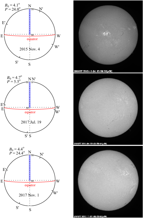
Figure 1.: Left panels: Graphical description of the observed points on the solar disk, (32 points on the northern meridian from the disk center to $0.97{\rm R}_{\odot}$ with a step of $30^{\prime\prime}\approx 0.03{\rm R}_{\odot}$, while spatially averaged over $50^{\prime\prime}$ along the E–W direction) at which the spectral data obtained in this study were taken. Shown are the three configurations of the Sun on the mid-dates of three different observing seasons (2015 November, 2017 July, and 2017 November). N, S, E, and W are the directions in reference to the Sun (based on solar rotation), whereas those in the equatorial coordinate system on the celestial sphere (defined by the rotation of Earth) are also denoted as N^′, S^′, E^′, and W^′. Right panels: Corresponding H$\alpha$ full-disk images of the Sun on these dates, which were observed by Solar Magnetic Activity Research Telescope (SMART) at Hida observatory.

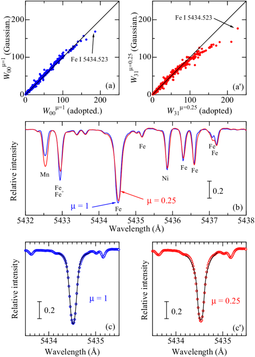
Figure 2.: Upper panels (a) and (a^′): comparison of the finally obtained equivalent widths (abscissa) with those measured by the Gaussian-fitting technique (ordinate), where left (a) and right (a^′) panels are for the disk center (point 00; $\mu=1$) and nearest to the limb (point 31; $\mu=0.25$), respectively. Middle panel (b): Comparison of disk-center spectrum ($\mu=1$: blue line) with the nearest-to-limb one ($\mu=0.25$: red line) in the 5432–5438 Å region. Lower panels (c) and (c^′): Comparison of the theoretically modeled profile (lines) of Fe i 5434.523, which is best-fitted with the observed one (symbols) for $\mu=1$ (left) and $\mu=0.25$ (right) cases.

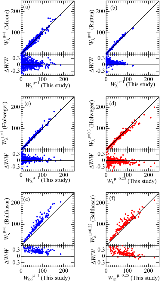
Figure 3.: Our equivalent widths are compared with those taken from four representative publications, where not only the direct comparison [$W_{\rm other}$ vs. $W_{\rm our}$; upper panel] but also the behaviors of relative differences [$(W_{\rm other}-W_{\rm our})/W_{\rm our}$ vs. $W_{\rm our}$; lower panel] are shown. The figure panels with blue symbols are for $\mu=1$ (disk center), while those with red symbols are for $\mu=$ 0.2–0.3 (near the limb). (a) Moore, Minnaert, and Houtgast (1966). (b) Rutten and van der Zalm (1984a) (their background-corrected $W^{\rm T}$ values were used). (c),(d) Holweger (1967). (e),(f) Balthasar (1988).

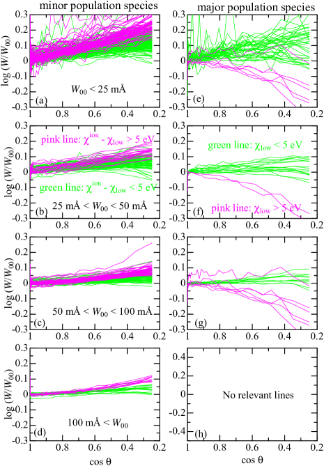
Figure 4.: Behaviors of $\log(W/W_{00})$ (equivalent width ratio normalized by the disk-center value) plotted against $\cos\theta$. The left panels (a)–(d) and the right panels (e)–(h) are for the lines of minor population stage (e.g., Fe i) and those of major population stage (e.g., C i, Fe ii), respectively. Lines are divided into four groups according to the range of $W_{00}$: $W_{00}<25$ mÅ (a,e), 25 mÅ $\leq W_{00}<50$ mÅ (b,f), 50 mÅ $\leq W_{00}<100$ mÅ (c,g), and 100 mÅ $\leq W_{00}$ (d,h). In each panel, lines are also discriminated into two classes and plotted in different colors according to the relevant key potential energy: For left panels (a–d: minor population), $\chi^{\rm ion}-\chi_{\rm low}<5$ eV (green) and $\chi^{\rm ion}-\chi_{\rm low}>5$ eV (pink). For right panels (e–h: major population), $\chi_{\rm low}<5$ eV (green) and $\chi_{\rm low}>5$ eV (pink).

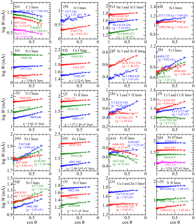
Figure 5.: The $\log W$ values of various representative lines are plotted against $\cos\theta$ in order to demonstrate their center–limb variations. The spectral lines displayed in each panel are appropriately selected in order to clarify the characteristic trends in terms of the species, excitation potentials, and line strengths. The observed data are shown by open circles while the corresponding linear-regression lines (cf. Equation 7) are depicted by solid lines.

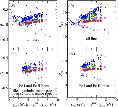
Figure 6.: The behaviors of $\beta$ (left panels (a) and (a^′)) and $K_{00}$ (right panels (b) and (b^′)) plotted against $\chi_{\rm low}$ (for major population species) or $\chi^{\rm ion}-\chi_{\rm low}$ (for minor population species). The upper panels (a) and (b) show the results of all lines, while the lower panels (a^′) and (b^′) display those for Fe i and Fe ii lines. The filled and open symbols correspond to minor population and major population species, respectively. Lines of different strengths classes are discriminated by the shape and the size (larger for stronger lines) of symbols: circles (blue): $W_{00}<$ 25 mÅ  triangles (green): 25 mÅ $\leq W_{00}<$ 50 mÅ  squares (pink): 50 mÅ $\leq W_{00}<$ 100 mÅ  and diamonds (brown): 100 mÅ $\leq W_{00}$.

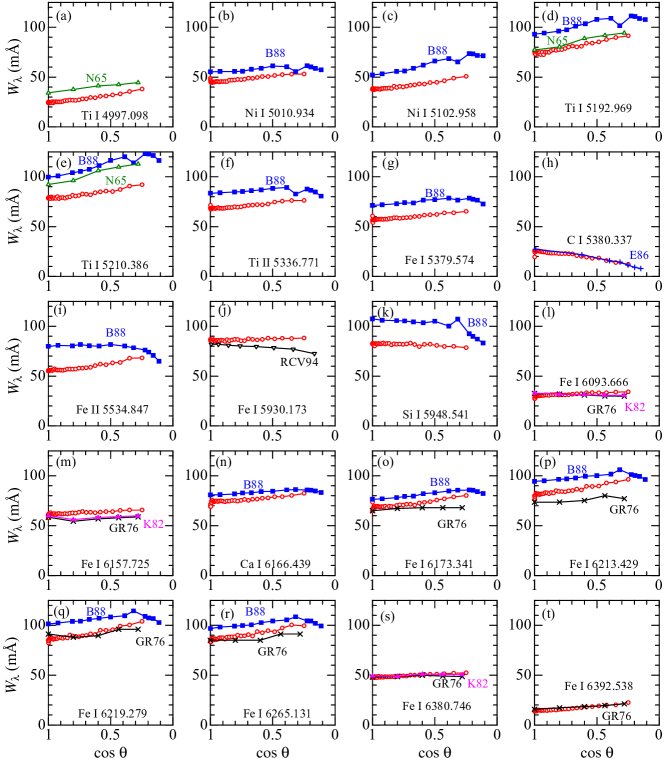
Figure 7.: In each panel are compared our $W$ vs. $\cos\theta$ relations derived for 20 lines (open circles) with those published by previous studies. N65 (green open triangles): Nissen (1965), GR76 (black St Andrew’s crosses): Gurtovenko and Ratnikova (1976), K82 (pink filled triangles): Kostik (1982), E86 (blue Greek crosses): Elste (1986), B88 (blue filled squares): Balthasar (1988), and RCV94 (black open inverse triangles): Rodríguez Hidalgo, Collados, and Vázquez (1994).

Table 1.: Observed points on the solar disk.

No.	$\sin\theta$	$\cos\theta$	$\theta$		No.	$\sin\theta$	$\cos\theta$	$\theta$
(1)	(2)	(3)	(4)		(1)	(2)	(3)	(4)
00	0.000	1.000	0.0		16	0.500	0.866	30.0
01	0.031	1.000	1.8		17	0.531	0.847	32.1
02	0.063	0.998	3.6		18	0.563	0.827	34.2
03	0.094	0.996	5.4		19	0.594	0.805	36.4
04	0.125	0.992	7.2		20	0.625	0.781	38.7
05	0.156	0.988	9.0		21	0.656	0.755	41.0
06	0.188	0.982	10.8		22	0.688	0.726	43.4
07	0.219	0.976	12.6		23	0.719	0.695	46.0
08	0.250	0.968	14.5		24	0.750	0.661	48.6
09	0.281	0.960	16.3		25	0.781	0.624	51.4
10	0.313	0.950	18.2		26	0.813	0.583	54.3
11	0.344	0.939	20.1		27	0.844	0.537	57.5
12	0.375	0.927	22.0		28	0.875	0.484	61.0
13	0.406	0.914	24.0		29	0.906	0.423	65.0
14	0.438	0.899	25.9		30	0.938	0.348	69.6
15	0.469	0.883	28.0		31	0.969	0.248	75.6

(1) Designated number of each observed point (cf. Figure 1). (2) Value of $\sin\theta$ (equivalent to the concentric radius in unit of the solar radius), where $\theta$ is the angle between the line of sight and the normal to the surface. (3) Value of $\cos\theta$, which is often referred to as $\mu$. (4) Value of $\theta$ (in deg). Note that all the values given here correspond to the positions just on the meridian. Since our spectra were derived by spatially averaging along the direction of the slit (perpendicular to the meridian) by $\approx\pm 25^{\prime\prime}$ (cf. Section 2), light from slightly different (larger) angle is actually included: i.e., up to $\theta^{\prime}(>\theta)$ where $\sin\theta^{\prime}\equiv\sqrt{\sin^{2}\theta+(25/960)^{2}}$. Nevertheless, this effect is insignificant, which is barely detectable only near the disk center of small $\theta$; e.g., $\sin\theta^{\prime}-\sin\theta$ is 0.026 (No. 00), 0.010 (No. 01), 0.005 (No. 02), 0.002 (No. 05), and 0.001 (No. 10).

Table 2.: Wavelength regions and observed dates of the spectra.

Region	$\lambda_{\rm min}$	$\lambda_{\rm max}$	Date		Region	$\lambda_{\rm min}$	$\lambda_{\rm max}$	Date
(1)	(2)	(3)	(4)		(1)	(2)	(3)	(4)
w4700	4687.5	4712.3	171103		w5800	5788.8	5811.1	170720
w4720	4707.6	4732.4	171103		w5820	5808.7	5831.0	170720
w4740	4727.7	4752.5	171103		w5840	5827.7	5851.7	151104
w4760	4747.7	4772.4	171103		w5860	5847.9	5871.9	151104
w4780	4767.5	4792.3	171103		w5880	5868.1	5892.1	171101
w4800	4787.6	4812.4	171103		w5900	5888.0	5912.0	171101
w4820	4807.5	4832.2	171103		w5920	5907.9	5931.9	171101
w4840	4827.4	4852.1	171103		w5940	5927.9	5951.9	171101
w4860	4847.6	4872.3	171103		w5960	5948.0	5972.0	171102
w4880	4867.7	4892.4	171102		w5980	5968.0	5991.9	171102
w4900	4887.7	4912.4	171102		w6000	5987.8	6011.7	171102
w4920	4907.7	4932.4	171102		w6020	6007.8	6031.7	171102
w4940	4927.6	4952.3	171102		w6040	6027.9	6051.8	171102
w4960	4947.8	4972.4	171102		w6060	6048.3	6072.2	151104
w4980	4967.8	4992.4	171102		w6080	6068.1	6091.9	151104
w5000	4988.7	5011.5	170719		w6100	6088.0	6111.9	151104
w5020	5008.6	5031.4	170719		w6120	6108.1	6131.9	151104
w5040	5028.5	5051.3	170719		w6140	6127.9	6151.7	151104
w5060	5048.5	5071.3	170719		w6160	6148.1	6171.9	151104
w5080	5068.4	5091.2	170719		w6180	6168.1	6191.8	151104
w5100	5088.6	5111.3	170719		w6200	6188.1	6211.9	151105
w5120	5108.8	5131.6	170719		w6220	6208.4	6232.1	151105
w5140	5128.3	5151.0	170719		w6240	6228.1	6251.9	151105
w5160	5148.5	5171.2	170719		w6260	6248.0	6271.8	151105
w5180	5168.5	5191.2	170717		w6280	6268.1	6291.8	151105
w5200	5188.3	5211.0	170717		w6300	6288.1	6311.8	151105
w5220	5207.8	5232.3	151103		w6320	6309.3	6331.3	170721
w5240	5227.7	5252.1	151103		w6340	6329.1	6351.0	170721
w5260	5248.3	5272.7	151103		w6360	6349.2	6371.1	170721
w5280	5267.9	5292.3	151103		w6380	6369.1	6391.0	170721
w5300	5287.8	5312.2	151103		w6400	6389.1	6410.9	170721
w5320	5307.8	5332.2	151104		w6420	6409.0	6430.9	170721
w5340	5327.8	5352.1	151104		w6440	6428.9	6450.7	170721
w5360	5347.5	5371.9	151104		w6460	6449.0	6470.9	170721
w5380	5367.9	5392.2	151104		w6480	6469.2	6491.1	170721
w5400	5387.8	5412.2	151104		w6500	6488.9	6510.7	170721
w5420	5408.0	5432.3	151104		w6520	6509.2	6531.0	170721
w5440	5427.7	5452.0	151104		w6540	6528.4	6551.9	171031
w5460	5448.8	5471.3	170719		w6560	6548.3	6571.8	171031
w5480	5468.7	5491.2	170719		w6580	6568.4	6591.9	171031
w5500	5488.6	5511.1	170719		w6600	6588.0	6611.5	171031
w5520	5508.7	5531.2	170719		w6620	6607.7	6631.1	171031
w5540	5528.4	5550.9	170719		w6640	6628.3	6651.7	171031
w5560	5548.8	5571.2	170719		w6660	6648.2	6671.6	171031
w5580	5568.7	5591.1	170719		w6680	6667.9	6691.3	171031
w5600	5588.2	5610.7	170720		w6700	6688.0	6711.4	171031
w5620	5608.5	5630.9	170720		w6720	6708.3	6731.6	171031
w5640	5629.0	5651.4	170720		w6740	6728.1	6751.4	171031
w5660	5648.0	5672.1	151104		w6760	6748.0	6771.4	171031
w5680	5668.1	5692.2	151104		w6780	6768.8	6792.0	171031
w5700	5689.1	5711.5	170720		w6800	6788.3	6811.6	171031
w5720	5708.8	5731.2	170720		w6820	6808.4	6831.7	171031
w5740	5728.8	5751.1	170720		w6840	6828.2	6851.4	171031
w5760	5748.7	5771.0	170720		w6860	6847.9	6871.2	171031
w5780	5769.0	5791.3	170720

(1) Region name. (2) Minimum wavelength (in Å). (3) Maximum wavelength (in Å). (4) Observed date expressed as $yymmdd$ (e.g., “171103” means that the spectrum was observed on 2017 November 3).

Table 3.: Data of the spectral lines and strength-related parameters. [1/10]

s-code	$\lambda$	$\chi_{\rm low}$	$\log gf$	$\log\epsilon_{00}$	$W_{00}$	$W_{31}$	$K_{00}$	$\alpha$	$\beta$
(1)	(2)	(3)	(4)	(5)	(6)	(7)	(8)	(9)	(10)
[C i lines, $\chi^{\rm ion}$ =11.26 eV, major population stage]
6.00	5052.167	7.68	$-$1.65	8.73	35.8	19.3	+4.36	1.269	$-$0.302
6.00	5380.337	7.68	$-$1.84	8.71	25.7	12.1	+4.11	1.067	$-$0.346
6.00	6587.610	8.54	$-$1.60	8.97	17.9	7.6	+5.99	0.884	$-$0.391
6.00	6655.517	8.54	$-$1.37	8.06	4.7	2.6	+6.84	0.398	$-$0.274
[O i lines, $\chi^{\rm ion}$ =13.62 eV, major population stage]
8.00	a5577.339	1.97	$-$8.20	9.30	4.9	7.1	0.00	0.897	+0.252
8.00	b6363.776	0.02	$-$10.30	9.13	2.1	3.0	$-$2.75	0.517	+0.196
[Na i lines, $\chi^{\rm ion}$ = 5.14 eV, minor population stage]
11.00	6154.226	2.10	$-$1.56	6.24	32.2	42.0	$-$5.27	1.659	+0.121
11.00	6160.747	2.10	$-$1.26	6.27	53.4	65.0	$-$4.26	1.837	+0.082
[Al i lines, $\chi^{\rm ion}$ = 5.99 eV, minor population stage]
13.00	6698.673	3.14	$-$1.65	6.19	18.5	23.5	$-$5.45	1.406	+0.147
[Si i lines, $\chi^{\rm ion}$ = 8.15 eV, minor population stage]
14.00	5398.845	5.61	$-$3.04	7.95	$\cdots$	5.0	$-$2.84	0.734	+0.232
14.00	5488.983	5.61	$-$0.53	6.14	14.3	18.5	$-$2.23	1.357	+0.198
14.00	5517.533	5.08	$-$2.38	7.45	11.9	14.6	$-$2.68	1.204	+0.122
14.00	5684.484	4.95	$-$1.65	7.60	62.9	62.1	$-$1.71	1.820	+0.018
14.00	5753.623	5.62	$-$0.83	7.11	47.8	54.6	$-$1.58	1.781	+0.093
14.00	5873.764	4.93	$-$2.61	7.11	4.9	5.8	$-$2.98	0.850	+0.164
14.00	5948.541	5.08	$-$1.23	7.52	82.3	78.5	$-$1.30	1.896	$-$0.021
14.00	6067.624	5.08	$-$2.98	7.36	2.8	3.8	$-$4.13	0.616	+0.141
14.00	6112.928	5.62	$-$1.75	7.08	8.0	10.3	$-$2.19	1.072	+0.128
14.00	6125.021	5.61	$-$0.93	6.92	29.7	31.4	$-$1.86	1.558	+0.059
14.00	6142.483	5.62	$-$0.92	6.99	33.9	33.4	$-$1.72	1.572	+0.010
14.00	6145.016	5.62	$-$0.82	6.97	38.7	36.6	$-$1.65	1.601	$-$0.016
14.00	6155.693	5.62	$-$1.69	6.85	5.5	7.2	$-$2.65	0.929	+0.156
14.00	6243.815	5.62	$-$0.77	7.05	47.1	42.4	$-$1.54	1.672	$-$0.015
14.00	6244.466	5.62	$-$0.69	6.94	45.1	42.2	$-$1.54	1.672	+0.004
14.00	6308.825	5.86	$-$2.95	8.41	6.8	7.3	$-$2.14	0.931	+0.086
14.00	6310.280	5.96	$-$1.82	7.77	16.1	17.4	$-$1.62	1.307	+0.092
14.00	6616.124	5.95	$-$2.85	7.73	1.6	1.7	$-$1.86	0.265	+0.078
14.00	6721.848	5.86	$-$1.49	7.89	47.4	42.1	$-$1.35	1.647	$-$0.036
14.00	6741.628	5.98	$-$1.75	7.64	14.1	13.5	$-$1.45	1.181	+0.032
14.00	6795.788	5.96	$-$1.98	7.72	10.6	14.3	$-$1.65	1.291	+0.268
14.00	6800.596	5.96	$-$1.64	7.40	11.1	11.4	$-$1.58	1.102	+0.048
14.00	6848.580	5.86	$-$2.08	7.92	15.8	15.3	$-$1.65	1.242	+0.035
[Ca i lines, $\chi^{\rm ion}$ = 6.11 eV, minor population stage]
20.00	5260.387	2.52	$-$1.90	6.55	32.5	38.3	$-$5.59	1.626	+0.122
20.00	5349.465	2.71	$-$1.18	7.13	90.5	103.3	$-$2.27	2.025	+0.071
20.00	5512.980	2.93	$-$0.29	6.13	89.1	94.2	$-$2.69	1.974	+0.024
20.00	5581.965	2.52	$-$0.71	6.35	85.8	96.8	$-$2.52	1.985	+0.057
20.00	5590.114	2.52	$-$0.71	6.32	84.4	100.4	$-$2.57	1.999	+0.078
20.00	5867.562	2.93	$-$0.80	5.55	22.1	28.6	$-$5.99	1.505	+0.130
20.00	6161.297	2.52	$-$1.02	6.05	58.8	71.0	$-$4.08	1.869	+0.079
20.00	6166.439	2.52	$-$0.90	6.10	69.1	82.3	$-$3.55	1.929	+0.067
20.00	6169.042	2.52	$-$0.55	6.08	89.8	113.4	$-$2.99	2.047	+0.080
20.00	6169.563	2.53	$-$0.27	6.16	115.3	$\cdots$	$-$2.85	2.153	+0.085
20.00	6455.598	2.52	$-$1.35	6.29	52.4	60.7	$-$4.30	1.803	+0.086
20.00	6499.650	2.52	$-$0.59	5.99	79.3	93.1	$-$2.95	1.969	+0.074
[Sc i lines, $\chi^{\rm ion}$ = 6.54 eV, minor population stage]
21.00	5356.091	1.86	+0.12	3.08	1.8	2.9	$-$10.94	0.511	+0.197
21.00	5392.078	1.99	$-$0.01	3.78	5.1	10.9	$-$10.00	1.260	+0.455
21.00	5484.626	1.85	+0.08	3.21	2.4	3.1	$-$9.63	0.580	+0.210
[Sc ii lines, $\chi^{\rm ion}$ =12.80 eV, major population stage]
21.01	5239.813	1.46	$-$0.77	3.01	41.0	49.5	$-$0.42	1.718	+0.110
21.01	5318.349	1.36	$-$2.04	3.25	7.9	11.4	$-$1.10	1.103	+0.216
21.01	5526.790	1.77	+0.13	2.99	72.1	81.8	$-$0.12	1.927	+0.070
21.01	5552.224	1.46	$-$2.27	3.21	3.7	5.5	$-$0.77	0.811	+0.243
21.01	5667.149	1.50	$-$1.24	3.20	26.6	32.9	$-$0.54	1.585	+0.145
21.01	5669.042	1.50	$-$1.12	3.15	29.8	36.2	$-$0.49	1.611	+0.129
21.01	5684.202	1.51	$-$1.05	3.17	33.7	42.7	$-$0.34	1.671	+0.136
21.01	6245.637	1.51	$-$0.98	3.04	32.9	38.4	$-$0.44	1.636	+0.112
21.01	6320.851	1.50	$-$1.77	2.96	6.5	10.0	$-$0.89	1.063	+0.238
[Ti i lines, $\chi^{\rm ion}$ = 6.82 eV, minor population stage]
22.00	4742.792	2.24	+0.21	4.80	26.3	33.8	$-$7.42	1.580	+0.159
22.00	4758.120	2.25	+0.42	4.90	40.5	45.9	$-$5.77	1.704	+0.101
22.00	4759.272	2.26	+0.51	4.90	44.8	51.0	$-$5.22	1.746	+0.099
22.00	4856.012	2.26	+0.44	4.89	38.4	50.5	$-$6.69	1.798	+0.208

^aPartially blended with C₂ lines (cf. Section 3.2).
^bPartially blended with CN line (cf. Section 3.2).

Table 3.: (Continued.) [2/10]

s-code	$\lambda$	$\chi_{\rm low}$	$\log gf$	$\log\epsilon_{00}$	$W_{00}$	$W_{31}$	$K_{00}$	$\alpha$	$\beta$
(1)	(2)	(3)	(4)	(5)	(6)	(7)	(8)	(9)	(10)
22.00	4926.147	0.82	$-$2.17	4.98	5.3	10.3	$-$12.84	1.072	+0.355
22.00	4997.098	0.00	$-$2.12	4.87	24.1	37.9	$-$11.80	1.627	+0.245
22.00	4999.504	0.83	+0.25	4.84	95.3	118.6	$-$3.21	2.088	+0.110
22.00	5009.646	0.02	$-$2.26	4.90	19.0	31.5	$-$12.63	1.546	+0.268
22.00	5016.162	0.85	$-$0.57	4.87	58.6	67.7	$-$5.17	1.853	+0.112
22.00	5022.871	0.83	$-$0.43	4.92	68.7	80.8	$-$4.21	1.930	+0.117
22.00	5024.842	0.82	$-$0.60	5.03	66.5	82.0	$-$4.43	1.941	+0.142
22.00	5036.468	1.44	+0.13	4.73	58.2	67.8	$-$4.71	1.853	+0.086
22.00	5039.959	0.02	$-$1.13	4.78	67.0	83.9	$-$4.92	1.937	+0.114
22.00	5043.588	0.84	$-$1.73	4.81	9.1	17.0	$-$12.67	1.252	+0.296
22.00	5062.112	2.16	$-$0.46	4.97	12.7	17.9	$-$9.22	1.310	+0.207
22.00	5064.081	2.69	$-$0.27	4.82	4.8	7.5	$-$8.94	0.947	+0.267
22.00	5064.654	0.05	$-$0.99	4.69	68.4	80.1	$-$4.78	1.906	+0.076
22.00	5113.448	1.44	$-$0.78	4.94	23.9	38.2	$-$9.21	1.658	+0.277
22.00	5147.479	0.00	$-$2.01	4.94	32.7	45.2	$-$10.41	1.681	+0.183
22.00	5152.185	0.02	$-$2.02	4.93	30.7	46.0	$-$10.81	1.707	+0.227
22.00	5173.742	0.00	$-$1.12	4.87	73.8	88.7	$-$4.43	1.965	+0.104
22.00	5192.969	0.02	$-$1.01	4.82	75.7	91.4	$-$4.28	1.991	+0.124
22.00	5210.386	0.05	$-$0.88	4.78	78.5	92.0	$-$4.12	1.978	+0.087
22.00	5219.700	0.02	$-$2.29	4.99	21.8	36.0	$-$12.34	1.608	+0.273
22.00	5247.291	2.10	$-$0.73	4.88	7.0	11.7	$-$9.77	1.125	+0.289
22.00	5260.001	2.74	$-$0.18	4.84	5.7	8.0	$-$8.97	0.958	+0.203
22.00	5295.780	1.07	$-$1.63	4.95	9.9	15.7	$-$12.02	1.268	+0.273
22.00	5384.631	0.83	$-$2.91	4.97	1.1	2.7	$-$13.76	0.655	+0.551
22.00	5426.237	0.02	$-$3.01	4.94	4.8	9.8	$-$14.60	1.059	+0.347
22.00	5453.643	1.44	$-$1.61	4.81	3.6	6.4	$-$11.88	0.830	+0.291
22.00	5471.197	1.44	$-$1.40	4.87	6.5	10.3	$-$11.73	1.097	+0.287
22.00	5490.150	1.46	$-$0.93	4.91	17.8	25.0	$-$10.22	1.445	+0.191
22.00	5503.897	2.58	+0.02	4.81	11.6	15.6	$-$8.61	1.241	+0.172
22.00	5648.567	2.50	$-$0.26	4.86	8.5	11.8	$-$9.02	1.146	+0.204
22.00	5716.457	2.30	$-$0.70	4.84	4.9	7.0	$-$9.93	0.934	+0.250
22.00	5739.464	2.25	$-$0.60	4.81	6.2	9.2	$-$10.09	1.050	+0.263
22.00	5866.452	1.07	$-$0.84	4.91	40.4	57.4	$-$7.97	1.809	+0.164
22.00	5880.273	1.05	$-$2.04	4.96	4.8	7.8	$-$12.98	0.971	+0.305
22.00	5903.317	1.07	$-$2.15	4.87	3.0	9.1	$-$13.05	1.059	+0.559
22.00	5922.110	1.05	$-$1.47	5.00	17.5	27.0	$-$11.17	1.489	+0.257
22.00	5965.828	1.88	$-$0.41	4.82	19.9	27.2	$-$9.32	1.463	+0.153
22.00	5978.543	1.87	$-$0.50	4.89	19.4	27.3	$-$9.27	1.471	+0.170
22.00	6031.677	0.05	$-$4.17	5.23	0.7	1.2	$-$16.51	0.110	+0.298
22.00	6064.629	1.05	$-$1.94	4.94	6.0	12.2	$-$12.32	1.137	+0.323
22.00	6092.798	1.89	$-$1.38	4.97	3.6	6.3	$-$10.94	0.866	+0.285
22.00	6098.694	3.06	$-$0.01	4.83	4.7	7.0	$-$8.61	0.898	+0.183
22.00	6121.006	1.88	$-$0.91	4.28	2.3	3.3	$-$11.07	0.632	+0.242
22.00	6126.217	1.07	$-$1.43	4.95	17.2	28.0	$-$11.23	1.524	+0.250
22.00	6220.500	2.68	$-$0.14	4.76	6.7	9.6	$-$8.86	1.092	+0.252
22.00	6258.104	1.44	$-$0.35	4.89	48.0	60.2	$-$6.61	1.813	+0.125
22.00	6303.757	1.44	$-$1.57	5.00	6.8	10.1	$-$11.73	1.084	+0.262
22.00	6312.238	1.46	$-$1.55	4.86	5.0	9.2	$-$11.78	1.006	+0.294
22.00	6419.098	2.17	$-$1.50	4.90	1.3	2.1	$-$10.70	0.345	+0.238
22.00	6716.707	2.49	$-$1.39	5.19	1.7	2.6	$-$9.63	0.483	+0.257
22.00	6743.124	0.90	$-$1.63	4.83	13.4	21.4	$-$11.98	1.383	+0.254
22.00	6746.313	1.89	$-$4.02	6.84	0.7	0.9	$-$8.26	$-$0.041	+0.126
[Ti ii lines, $\chi^{\rm ion}$ =13.58 eV, major population stage]
22.01	5005.157	1.57	$-$2.55	4.80	19.3	25.9	$-$0.60	1.460	+0.171
22.01	5185.913	1.89	$-$1.35	4.79	60.5	63.0	0.00	1.807	+0.027
22.01	5211.536	2.59	$-$1.36	4.84	31.0	33.5	+0.56	1.553	+0.066
22.01	5336.771	1.58	$-$1.70	5.00	68.5	76.1	$-$0.21	1.900	+0.068
22.01	5381.015	1.57	$-$2.08	5.01	51.5	56.3	$-$0.17	1.782	+0.070
22.01	5418.751	1.58	$-$2.00	4.81	45.0	53.2	$-$0.26	1.760	+0.103
[V i line, $\chi^{\rm ion}$ = 6.74 eV, minor population stage]
23.00	5657.435	1.06	$-$1.02	3.93	4.5	7.5	$-$12.57	0.947	+0.255
23.00	5668.361	1.08	$-$1.03	4.03	5.3	9.4	$-$12.20	0.987	+0.232

Table 3.: (Continued.) [3/10]

s-code	$\lambda$	$\chi_{\rm low}$	$\log gf$	$\log\epsilon_{00}$	$W_{00}$	$W_{31}$	$K_{00}$	$\alpha$	$\beta$
(1)	(2)	(3)	(4)	(5)	(6)	(7)	(8)	(9)	(10)
23.00	5670.853	1.08	$-$0.42	3.96	16.1	24.4	$-$11.07	1.427	+0.199
23.00	6058.139	1.04	$-$1.37	4.13	3.5	5.7	$-$13.46	0.803	+0.232
23.00	6111.645	1.04	$-$0.71	3.90	9.2	14.1	$-$12.54	1.236	+0.239
23.00	6135.361	1.05	$-$0.75	3.85	7.6	13.3	$-$12.60	1.198	+0.274
23.00	6150.157	0.30	$-$1.78	4.01	5.7	11.3	$-$14.33	1.148	+0.323
23.00	6224.529	0.29	$-$2.01	4.06	4.0	6.8	$-$14.62	0.909	+0.305
23.00	6233.164	0.28	$-$2.07	3.97	3.0	5.8	$-$14.21	0.830	+0.347
23.00	6242.829	0.26	$-$1.55	3.89	8.0	14.3	$-$13.93	1.228	+0.309
23.00	6251.827	0.29	$-$1.34	3.92	12.5	21.7	$-$13.55	1.403	+0.296
23.00	6266.307	0.28	$-$2.29	4.11	2.5	4.0	$-$14.73	0.690	+0.284
23.00	6274.649	0.27	$-$1.67	3.91	6.4	13.1	$-$14.34	1.177	+0.375
23.00	6326.840	1.87	$-$0.81	3.89	1.3	1.7	$-$13.34	0.283	+0.173
23.00	6531.415	1.22	$-$0.84	3.93	5.5	8.5	$-$12.79	0.992	+0.262
[V ii line, $\chi^{\rm ion}$ =14.65 eV, major population stage]
23.01	5303.255	2.28	$-$1.94	3.84	2.9	2.6	0.00	0.507	+0.018
[Cr i lines, $\chi^{\rm ion}$ = 6.77 eV, minor population stage]
24.00	4708.018	3.17	+0.11	5.60	53.8	57.4	$-$3.60	1.789	+0.060
24.00	4756.137	3.10	+0.09	5.76	61.7	68.1	$-$2.95	1.856	+0.070
24.00	4801.047	3.12	$-$0.13	5.65	46.1	53.4	$-$4.20	1.753	+0.089
24.00	4964.916	0.94	$-$2.53	5.69	35.0	55.4	$-$8.54	1.790	+0.254
24.00	4966.810	3.85	$-$0.95	5.63	3.1	3.5	$-$6.42	0.610	+0.105
24.00	5200.207	3.38	$-$0.66	6.02	29.1	36.8	$-$5.74	1.656	+0.191
24.00	5238.964	2.71	$-$1.30	5.61	14.0	18.8	$-$8.37	1.337	+0.195
24.00	5247.566	0.96	$-$1.64	5.73	80.2	95.6	$-$3.64	2.002	+0.108
24.00	5272.007	3.45	$-$0.42	5.64	20.9	26.3	$-$6.33	1.454	+0.130
24.00	5275.713	2.89	$-$0.05	5.49	70.7	76.8	$-$3.96	1.882	+0.038
24.00	5293.396	3.38	$-$1.36	5.68	3.9	5.2	$-$8.05	0.765	+0.165
24.00	5296.691	0.98	$-$1.40	5.75	91.4	111.9	$-$3.35	2.056	+0.101
24.00	5297.968	2.90	$-$0.06	5.61	71.7	73.3	$-$3.38	1.861	+0.012
24.00	5300.744	0.98	$-$2.12	5.68	55.1	68.5	$-$5.66	1.851	+0.115
24.00	5312.871	3.45	$-$0.56	5.62	15.8	20.1	$-$6.70	1.327	+0.122
24.00	5329.142	2.91	$-$0.06	5.64	68.9	75.5	$-$3.31	1.888	+0.048
24.00	5340.472	3.44	$-$0.73	5.62	11.5	13.9	$-$7.26	1.203	+0.130
24.00	5344.789	3.45	$-$1.06	5.77	7.9	12.7	$-$7.32	1.137	+0.224
24.00	5348.312	1.00	$-$1.29	5.82	100.0	125.2	$-$3.32	2.106	+0.107
24.00	5729.178	3.85	$-$1.06	5.46	1.9	2.2	$-$7.81	0.409	+0.130
24.00	5787.965	3.32	$-$0.08	5.62	44.0	46.9	$-$4.79	1.697	+0.055
24.00	5844.593	3.01	$-$1.76	5.64	3.3	5.3	$-$8.50	0.722	+0.195
24.00	6047.672	3.85	$-$1.81	6.26	2.1	2.3	$-$8.26	0.368	+0.054
24.00	6135.734	4.82	$-$1.16	7.35	13.1	16.7	$-$4.65	1.291	+0.149
24.00	6330.093	0.94	$-$2.92	5.68	22.2	35.7	$-$10.89	1.606	+0.239
24.00	6630.005	1.03	$-$3.56	5.61	4.6	8.3	$-$13.05	0.963	+0.316
24.00	6636.317	4.14	$-$1.72	6.37	2.0	3.1	$-$7.41	0.523	+0.250
24.00	6661.078	4.19	$-$0.19	5.62	9.6	11.0	$-$5.96	1.093	+0.095
24.00	6669.255	4.17	$-$0.56	5.67	5.1	5.9	$-$6.80	0.837	+0.119
[Cr ii lines, $\chi^{\rm ion}$ =16.50 eV, major population stage]
24.01	5279.876	4.07	$-$2.10	5.78	17.7	20.4	+1.80	1.427	+0.159
24.01	5305.853	3.83	$-$2.36	6.00	24.2	22.9	+1.68	1.386	$-$0.001
24.01	5313.563	4.07	$-$1.65	5.72	32.1	32.5	+1.63	1.530	+0.022
24.01	5502.067	4.17	$-$1.99	5.68	15.8	15.1	+2.21	1.189	$-$0.017
24.01	6129.226	4.75	$-$2.44	5.89	3.6	3.4	+3.21	0.557	$-$0.034
[Mn i line, $\chi^{\rm ion}$ = 7.44 eV, minor population stage]
25.00	5004.892	2.92	$-$1.63	5.42	11.5	18.5	$-$8.47	1.314	+0.251
25.00	6265.612	4.23	$-$1.32	5.68	3.3	4.5	$-$7.01	0.717	+0.175
25.00	6391.200	4.27	$-$1.55	5.73	2.1	2.9	$-$7.05	0.532	+0.202
25.00	6440.971	3.77	$-$1.42	5.50	4.6	6.3	$-$8.08	0.856	+0.187
[Fe i lines, $\chi^{\rm ion}$ = 7.87 eV, minor population stage]
26.00	4690.136	3.69	$-$1.68	7.62	53.7	62.6	$-$3.34	1.820	+0.093
26.00	4741.529	2.83	$-$2.00	7.46	68.4	83.7	$-$2.96	1.939	+0.108
26.00	4779.443	3.42	$-$2.31	7.63	37.2	47.9	$-$5.13	1.719	+0.152
26.00	4780.811	3.25	$-$3.36	7.56	6.6	11.7	$-$8.63	1.136	+0.322
26.00	4785.957	4.14	$-$1.93	7.61	22.8	32.5	$-$5.44	1.560	+0.207
26.00	4790.746	3.25	$-$3.24	7.45	6.8	11.8	$-$8.86	1.148	+0.315
26.00	4807.708	3.37	$-$2.20	7.61	44.0	54.8	$-$4.67	1.765	+0.121
26.00	4808.147	3.25	$-$2.79	7.64	23.4	33.7	$-$6.89	1.574	+0.202

Table 3.: (Continued.) [4/10]

s-code	$\lambda$	$\chi_{\rm low}$	$\log gf$	$\log\epsilon_{00}$	$W_{00}$	$W_{31}$	$K_{00}$	$\alpha$	$\beta$
(1)	(2)	(3)	(4)	(5)	(6)	(7)	(8)	(9)	(10)
26.00	4813.116	3.27	$-$2.89	7.55	16.2	22.5	$-$7.80	1.395	+0.195
26.00	4835.869	4.10	$-$1.50	7.63	45.0	54.1	$-$3.79	1.766	+0.114
26.00	4882.144	3.42	$-$1.64	7.67	71.4	81.9	$-$2.91	1.925	+0.079
26.00	4907.733	3.43	$-$1.84	7.60	58.8	73.4	$-$3.39	1.879	+0.116
26.00	4939.686	0.86	$-$3.34	7.38	91.0	112.2	$-$3.27	2.069	+0.113
26.00	4950.104	3.42	$-$1.67	7.68	71.5	83.4	$-$2.91	1.943	+0.093
26.00	4961.915	3.63	$-$2.29	7.50	23.6	32.7	$-$6.23	1.567	+0.201
26.00	4962.565	4.18	$-$1.29	7.62	52.2	60.5	$-$3.21	1.806	+0.094
26.00	4969.916	4.22	$-$0.71	7.47	70.9	78.4	$-$2.32	1.910	+0.066
26.00	5001.862	3.88	+0.01	7.49	136.8	151.1	$-$3.01	2.190	+0.051
26.00	5002.789	3.40	$-$1.58	7.55	71.0	98.8	$-$2.89	2.013	+0.163
26.00	5014.941	3.94	$-$0.25	7.63	121.3	125.8	$-$2.78	2.120	+0.062
26.00	5022.236	3.98	$-$0.53	7.63	99.6	101.8	$-$2.47	2.029	+0.050
26.00	5028.126	3.57	$-$1.47	7.78	76.4	84.7	$-$2.50	1.944	+0.081
26.00	5072.076	4.28	$-$1.03	7.92	75.2	85.9	$-$2.31	1.961	+0.085
26.00	5074.748	4.22	$-$0.20	7.60	109.3	122.8	$-$2.09	2.091	+0.055
26.00	5079.739	0.99	$-$3.22	7.30	88.9	122.4	$-$3.28	2.087	+0.146
26.00	5083.338	0.96	$-$2.96	7.28	101.3	131.9	$-$3.25	2.125	+0.128
26.00	5123.719	1.01	$-$3.07	7.29	94.8	120.4	$-$3.23	2.078	+0.108
26.00	5127.358	0.92	$-$3.31	7.37	91.8	115.9	$-$3.30	2.064	+0.107
26.00	5127.681	0.05	$-$6.12	7.54	14.2	27.4	$-$14.10	1.482	+0.336
26.00	5137.395	4.18	$-$0.40	7.58	96.4	103.4	$-$2.13	1.999	+0.020
26.00	5145.094	2.20	$-$3.23	7.47	44.0	53.1	$-$5.98	1.736	+0.102
26.00	5159.050	4.28	$-$0.82	7.54	67.3	75.2	$-$2.40	1.885	+0.066
26.00	5194.941	1.56	$-$2.09	7.37	122.4	162.6	$-$3.43	2.233	+0.154
26.00	5195.468	4.22	0.00	7.34	103.1	115.0	$-$2.44	2.076	+0.071
26.00	5196.077	4.26	$-$0.45	7.23	71.8	79.6	$-$2.45	1.922	+0.076
26.00	5197.929	4.30	$-$1.64	7.64	31.5	38.4	$-$4.67	1.628	+0.141
26.00	5206.801	4.28	$-$2.53	7.51	4.7	6.9	$-$6.69	0.920	+0.259
26.00	5217.389	3.21	$-$1.10	7.62	114.6	132.8	$-$3.12	2.136	+0.080
26.00	5223.187	3.63	$-$2.39	7.65	26.7	34.3	$-$6.06	1.580	+0.158
26.00	5225.525	0.11	$-$4.79	7.43	66.9	89.2	$-$4.97	1.961	+0.143
26.00	5228.403	4.22	$-$1.29	7.67	54.0	58.9	$-$3.11	1.780	+0.053
26.00	5242.491	3.63	$-$0.84	7.39	85.7	96.3	$-$2.36	2.006	+0.080
26.00	5243.773	4.26	$-$1.15	7.67	60.0	66.3	$-$2.75	1.843	+0.071
26.00	5247.049	0.09	$-$4.95	7.46	62.4	81.0	$-$5.52	1.939	+0.157
26.00	5250.208	0.12	$-$4.94	7.46	61.1	84.0	$-$5.69	1.952	+0.179
26.00	5250.645	2.20	$-$2.05	7.44	98.3	126.7	$-$3.02	2.115	+0.135
26.00	5253.023	2.28	$-$3.94	7.58	15.3	24.6	$-$9.70	1.449	+0.274
26.00	5253.461	3.28	$-$1.67	7.55	73.5	87.8	$-$2.99	1.959	+0.101
26.00	5279.654	3.30	$-$3.44	7.39	3.7	5.8	$-$8.48	0.874	+0.293
26.00	5285.118	4.43	$-$1.64	7.56	23.1	31.9	$-$5.23	1.517	+0.155
26.00	5288.528	3.69	$-$1.67	7.50	51.1	54.8	$-$3.68	1.750	+0.041
26.00	5300.412	4.59	$-$1.75	6.92	3.8	5.2	$-$6.08	0.795	+0.214
26.00	5301.327	4.39	$-$2.75	7.50	2.3	3.7	$-$7.54	0.676	+0.307
26.00	5308.707	4.26	$-$2.50	7.46	4.8	6.3	$-$6.55	0.858	+0.172
26.00	5320.039	3.64	$-$2.54	7.53	16.6	25.0	$-$7.12	1.436	+0.216
26.00	5321.109	4.43	$-$1.44	7.66	36.6	41.8	$-$4.19	1.649	+0.085
26.00	5322.041	2.28	$-$3.03	7.53	53.7	66.2	$-$4.79	1.835	+0.107
26.00	5326.140	3.57	$-$1.55	6.83	30.5	37.7	$-$5.77	1.617	+0.133
26.00	5329.987	4.08	$-$1.30	7.46	49.4	52.8	$-$3.46	1.741	+0.049
26.00	5332.899	1.56	$-$2.94	7.53	89.2	108.0	$-$3.14	2.038	+0.092
26.00	5339.928	3.27	$-$0.68	7.64	148.2	170.2	$-$3.61	2.234	+0.067
26.00	5364.858	4.45	+0.22	7.70	131.6	133.4	$-$2.39	2.139	+0.018
26.00	5365.396	3.57	$-$1.44	7.60	72.1	81.1	$-$2.68	1.924	+0.067
26.00	5373.698	4.47	$-$0.86	7.58	60.1	65.2	$-$2.79	1.826	+0.045
26.00	5376.826	4.29	$-$2.31	7.76	12.5	18.7	$-$6.22	1.307	+0.206
26.00	5379.574	3.69	$-$1.48	7.41	56.3	65.2	$-$3.34	1.833	+0.082
26.00	5385.579	3.69	$-$2.97	7.39	4.8	7.4	$-$8.43	0.935	+0.261
26.00	5389.479	4.42	$-$0.41	7.54	82.5	93.2	$-$2.14	1.974	+0.058

Table 3.: (Continued.) [5/10]

s-code	$\lambda$	$\chi_{\rm low}$	$\log gf$	$\log\epsilon_{00}$	$W_{00}$	$W_{31}$	$K_{00}$	$\alpha$	$\beta$
(1)	(2)	(3)	(4)	(5)	(6)	(7)	(8)	(9)	(10)
26.00	5393.167	3.24	$-$0.91	7.76	140.3	157.4	$-$3.43	2.204	+0.057
26.00	5395.215	4.45	$-$2.17	7.91	16.6	22.3	$-$5.73	1.387	+0.154
26.00	5398.277	4.45	$-$0.67	7.57	70.8	76.9	$-$2.29	1.891	+0.038
26.00	5401.264	4.32	$-$1.92	7.68	21.5	27.1	$-$5.50	1.477	+0.135
26.00	5406.770	4.37	$-$1.72	7.77	32.0	38.6	$-$4.52	1.631	+0.113
26.00	5409.133	4.37	$-$1.30	7.71	49.7	54.8	$-$3.26	1.771	+0.065
26.00	5410.910	4.47	+0.28	7.61	127.5	127.9	$-$2.33	2.121	+0.018
26.00	5412.798	4.43	$-$1.89	7.68	18.6	24.9	$-$5.59	1.452	+0.170
26.00	5434.523	1.01	$-$2.12	7.48	186.4	227.6	$-$5.58	2.386	+0.126
26.00	5436.297	4.39	$-$1.54	7.66	34.0	40.2	$-$4.42	1.644	+0.102
26.00	5436.587	2.28	$-$3.39	7.49	34.3	47.1	$-$7.32	1.720	+0.171
26.00	5441.354	4.31	$-$1.73	7.63	27.3	32.8	$-$4.97	1.572	+0.124
26.00	5443.409	4.10	$-$2.95	7.36	2.0	3.0	$-$8.67	0.534	+0.233
26.00	5445.042	4.39	$-$0.02	7.68	121.6	121.4	$-$2.09	2.093	+0.010
26.00	5461.550	4.45	$-$1.90	7.78	21.8	27.4	$-$5.30	1.474	+0.138
26.00	5463.271	4.43	+0.11	7.32	98.7	109.0	$-$2.08	2.044	+0.048
26.00	5464.278	4.14	$-$1.72	7.62	34.4	41.6	$-$4.70	1.645	+0.111
26.00	5470.092	4.45	$-$1.81	7.62	19.2	23.4	$-$5.42	1.431	+0.148
26.00	5473.164	4.19	$-$2.14	7.65	17.1	21.2	$-$6.23	1.383	+0.152
26.00	5473.900	4.15	$-$0.76	7.49	77.0	89.0	$-$2.55	1.958	+0.076
26.00	5483.098	4.15	$-$1.58	7.64	42.5	47.8	$-$4.08	1.713	+0.088
26.00	5487.144	4.42	$-$1.53	7.59	30.6	33.9	$-$4.62	1.576	+0.090
26.00	5491.840	4.19	$-$2.40	7.62	9.9	29.9	$-$6.68	1.610	+0.641
26.00	5493.497	4.10	$-$1.84	7.79	39.4	55.7	$-$4.48	1.836	+0.240
26.00	5501.464	0.96	$-$2.95	7.16	101.1	125.1	$-$3.37	2.111	+0.113
26.00	5506.778	0.99	$-$2.80	7.40	120.7	157.8	$-$3.55	2.210	+0.135
26.00	5517.069	4.21	$-$2.37	7.80	14.2	18.7	$-$6.29	1.321	+0.161
26.00	5522.447	4.21	$-$1.55	7.61	39.9	45.5	$-$4.27	1.682	+0.079
26.00	5539.284	3.64	$-$2.66	7.52	13.3	19.1	$-$7.33	1.329	+0.209
26.00	5543.937	4.22	$-$1.14	7.59	59.4	64.5	$-$3.07	1.823	+0.053
26.00	5546.500	4.37	$-$1.31	7.69	47.7	52.6	$-$3.46	1.740	+0.065
26.00	5549.948	3.69	$-$2.91	7.59	8.4	11.2	$-$7.48	1.115	+0.193
26.00	5552.691	4.96	$-$1.99	7.78	7.3	8.8	$-$5.47	1.008	+0.144
26.00	5559.638	4.99	$-$1.83	7.55	6.0	7.1	$-$5.34	0.917	+0.144
26.00	5565.704	4.61	$-$0.28	7.52	81.9	86.9	$-$2.37	1.951	+0.042
26.00	5568.072	4.15	$-$1.76	6.29	2.4	3.4	$-$7.23	0.604	+0.235
26.00	5568.867	3.63	$-$2.95	7.56	8.2	11.8	$-$7.66	1.144	+0.235
26.00	5569.618	3.42	$-$0.54	7.66	155.4	179.3	$-$3.69	2.258	+0.071
26.00	5576.090	3.43	$-$1.00	7.73	118.0	127.1	$-$3.05	2.119	+0.049
26.00	5577.031	5.03	$-$1.55	7.58	10.6	12.2	$-$5.20	1.122	+0.098
26.00	5587.573	4.14	$-$1.85	7.71	33.4	41.3	$-$4.94	1.669	+0.151
26.00	5595.075	5.06	$-$1.77	7.47	4.9	6.5	$-$5.36	0.889	+0.201
26.00	5600.226	4.26	$-$1.81	7.65	27.6	32.5	$-$5.24	1.522	+0.080
26.00	5608.974	4.21	$-$2.40	7.57	8.6	11.8	$-$6.64	1.139	+0.201
26.00	5618.631	4.21	$-$1.38	7.56	46.2	51.8	$-$3.81	1.739	+0.077
26.00	5619.587	4.39	$-$1.70	7.71	29.9	35.4	$-$4.73	1.593	+0.117
26.00	5633.975	4.99	$-$0.27	7.49	62.5	63.3	$-$2.40	1.822	+0.024
26.00	5635.824	4.26	$-$1.89	7.79	30.3	36.0	$-$4.94	1.602	+0.116
26.00	5636.696	3.64	$-$2.61	7.54	15.7	21.9	$-$7.16	1.410	+0.211
26.00	5638.262	4.22	$-$0.87	7.58	73.6	81.3	$-$2.59	1.932	+0.065
26.00	5650.020	5.10	$-$0.92	7.67	35.7	37.7	$-$3.56	1.595	+0.038
26.00	5650.704	5.08	$-$0.96	7.73	34.8	38.6	$-$3.58	1.620	+0.070
26.00	5651.470	4.47	$-$2.00	7.74	16.4	21.3	$-$5.64	1.372	+0.144
26.00	5652.320	4.26	$-$1.95	7.70	23.9	30.5	$-$5.56	1.526	+0.138
26.00	5653.889	4.39	$-$1.64	7.73	34.2	40.4	$-$4.39	1.631	+0.091
26.00	5661.348	4.28	$-$2.02	7.67	19.2	25.1	$-$5.86	1.434	+0.144
26.00	5662.515	4.18	$-$0.54	7.61	96.8	110.1	$-$2.56	2.048	+0.063
26.00	5672.267	4.58	$-$2.80	7.43	1.2	1.5	$-$6.94	0.250	+0.138
26.00	5679.025	4.65	$-$0.92	7.76	58.8	63.6	$-$2.80	1.815	+0.040
26.00	5680.241	4.19	$-$2.58	7.73	8.7	12.2	$-$6.94	1.131	+0.181

Table 3.: (Continued.) [6/10]

s-code	$\lambda$	$\chi_{\rm low}$	$\log gf$	$\log\epsilon_{00}$	$W_{00}$	$W_{31}$	$K_{00}$	$\alpha$	$\beta$
(1)	(2)	(3)	(4)	(5)	(6)	(7)	(8)	(9)	(10)
26.00	5696.102	4.55	$-$1.99	7.50	9.1	11.5	$-$6.00	1.134	+0.166
26.00	5701.545	2.56	$-$2.22	7.52	80.9	92.1	$-$3.11	1.983	+0.077
26.00	5705.466	4.30	$-$1.60	7.63	34.9	39.8	$-$4.64	1.634	+0.092
26.00	5731.762	4.26	$-$1.30	7.65	53.6	60.6	$-$3.34	1.805	+0.079
26.00	5732.275	4.99	$-$1.56	7.61	11.9	15.1	$-$5.34	1.250	+0.177
26.00	5752.023	4.55	$-$1.27	7.82	49.7	55.1	$-$3.26	1.758	+0.061
26.00	5753.121	4.26	$-$0.76	7.48	72.0	79.8	$-$2.61	1.908	+0.052
26.00	5759.544	4.30	$-$2.22	7.46	8.5	11.8	$-$6.80	1.148	+0.213
26.00	5760.345	3.64	$-$2.49	7.53	19.3	26.9	$-$6.85	1.484	+0.194
26.00	5775.080	4.22	$-$1.20	7.57	56.5	62.6	$-$3.33	1.817	+0.067
26.00	5778.455	2.59	$-$3.59	7.50	15.6	24.8	$-$9.20	1.455	+0.269
26.00	5784.657	3.40	$-$2.67	7.55	22.1	30.1	$-$7.14	1.525	+0.183
26.00	5793.913	4.22	$-$1.70	7.53	29.2	35.3	$-$5.13	1.590	+0.122
26.00	5811.917	4.14	$-$2.43	7.54	8.9	12.5	$-$6.78	1.161	+0.204
26.00	5814.805	4.28	$-$1.97	7.61	19.3	24.9	$-$5.82	1.442	+0.152
26.00	5827.875	3.28	$-$3.41	7.71	9.0	13.2	$-$8.53	1.176	+0.219
26.00	5835.098	4.26	$-$2.37	7.72	11.7	15.7	$-$6.37	1.261	+0.177
26.00	5837.700	4.29	$-$2.34	7.57	8.5	10.9	$-$6.42	1.104	+0.165
26.00	5845.266	5.03	$-$1.82	7.52	5.3	7.9	$-$5.94	0.945	+0.199
26.00	5849.682	3.69	$-$2.99	7.50	6.0	9.7	$-$8.12	1.058	+0.244
26.00	5852.217	4.55	$-$1.33	7.60	35.6	43.2	$-$4.15	1.666	+0.087
26.00	5853.149	1.49	$-$5.28	7.53	4.6	10.8	$-$12.78	1.097	+0.371
26.00	5855.091	4.61	$-$1.76	7.68	18.6	25.4	$-$5.28	1.448	+0.148
26.00	5856.083	4.29	$-$1.64	7.53	28.8	37.0	$-$5.02	1.603	+0.115
26.00	5858.779	4.22	$-$2.26	7.61	12.5	17.5	$-$6.47	1.286	+0.153
26.00	5859.578	4.55	$-$0.40	7.36	74.2	80.5	$-$2.34	1.915	+0.030
26.00	5861.107	4.28	$-$2.45	7.52	6.2	9.9	$-$6.94	1.034	+0.206
26.00	5862.353	4.55	$-$0.06	7.31	89.6	93.7	$-$2.16	1.983	+0.018
26.00	5880.029	4.56	$-$1.94	7.61	12.6	15.8	$-$5.92	1.242	+0.139
26.00	5881.279	4.61	$-$1.84	7.46	10.4	14.1	$-$5.81	1.220	+0.217
26.00	5902.485	4.59	$-$1.81	7.49	12.0	15.1	$-$5.73	1.245	+0.150
26.00	5905.689	4.65	$-$0.73	7.41	51.3	53.8	$-$3.10	1.738	+0.024
26.00	5909.970	3.21	$-$2.78	7.50	23.4	29.5	$-$7.27	1.492	+0.129
26.00	5916.249	2.45	$-$2.99	7.52	49.5	60.5	$-$5.37	1.800	+0.113
26.00	5927.786	4.65	$-$1.09	7.54	39.3	46.0	$-$3.82	1.696	+0.102
26.00	5929.667	4.55	$-$1.41	7.70	36.4	40.2	$-$4.13	1.631	+0.072
26.00	5930.173	4.65	$-$0.23	7.59	86.2	88.2	$-$2.11	1.949	+0.016
26.00	5934.653	3.93	$-$1.17	7.53	71.2	74.7	$-$2.92	1.878	+0.029
26.00	5952.716	3.98	$-$1.44	7.52	52.5	60.9	$-$3.52	1.807	+0.077
26.00	5956.692	0.86	$-$4.61	7.51	47.7	65.0	$-$7.51	1.852	+0.166
26.00	5969.559	4.28	$-$2.73	7.48	3.1	4.4	$-$7.46	0.717	+0.194
26.00	5976.157	4.29	$-$2.55	6.87	1.1	1.8	$-$7.54	0.316	+0.253
26.00	5983.673	4.55	$-$1.88	8.72	66.8	72.9	$-$2.55	1.869	+0.038
26.00	5984.814	4.73	$-$0.34	7.54	76.8	79.6	$-$2.45	1.910	+0.018
26.00	5987.066	4.79	$-$0.56	7.67	68.6	71.6	$-$2.49	1.868	+0.025
26.00	6003.010	3.88	$-$1.12	7.61	80.7	89.9	$-$2.76	1.963	+0.047
26.00	6027.050	4.08	$-$1.21	7.60	64.0	67.4	$-$2.85	1.833	+0.035
26.00	6034.033	4.31	$-$2.42	7.56	6.9	10.1	$-$6.70	1.056	+0.212
26.00	6054.072	4.37	$-$2.31	7.55	7.7	11.1	$-$6.76	1.140	+0.228
26.00	6065.482	2.61	$-$1.53	7.62	125.6	153.2	$-$3.28	2.191	+0.092
26.00	6082.708	2.22	$-$3.57	7.42	27.5	42.4	$-$8.47	1.677	+0.194
26.00	6093.666	4.61	$-$1.50	7.65	27.9	34.2	$-$4.67	1.573	+0.103
26.00	6094.364	4.65	$-$1.94	7.83	16.6	21.5	$-$5.57	1.373	+0.126
26.00	6096.662	3.98	$-$1.93	7.60	33.4	42.5	$-$5.27	1.668	+0.117
26.00	6098.280	4.56	$-$1.88	7.58	13.7	19.0	$-$5.91	1.321	+0.153
26.00	6105.152	4.55	$-$2.05	7.54	9.2	12.0	$-$5.94	1.153	+0.161
26.00	6120.244	0.92	$-$5.95	7.40	2.9	6.1	$-$14.69	0.902	+0.404
26.00	6127.909	4.14	$-$0.72	6.77	44.4	52.2	$-$4.04	1.746	+0.073
26.00	6136.993	2.20	$-$2.95	7.35	57.6	75.1	$-$4.97	1.892	+0.103
26.00	6151.617	2.18	$-$3.30	7.41	43.0	60.3	$-$6.57	1.815	+0.144

Table 3.: (Continued.) [7/10]

s-code	$\lambda$	$\chi_{\rm low}$	$\log gf$	$\log\epsilon_{00}$	$W_{00}$	$W_{31}$	$K_{00}$	$\alpha$	$\beta$
(1)	(2)	(3)	(4)	(5)	(6)	(7)	(8)	(9)	(10)
26.00	6157.725	4.08	$-$1.26	7.51	57.7	65.6	$-$3.21	1.834	+0.049
26.00	6159.368	4.61	$-$1.97	7.58	10.6	14.9	$-$6.00	1.236	+0.176
26.00	6165.361	4.14	$-$1.55	7.54	41.1	49.1	$-$4.29	1.716	+0.072
26.00	6173.341	2.22	$-$2.88	7.44	64.7	80.2	$-$4.34	1.920	+0.090
26.00	6180.203	2.73	$-$2.78	7.50	47.1	59.8	$-$5.47	1.803	+0.107
26.00	6187.398	2.83	$-$4.34	7.67	3.0	5.1	$-$9.63	0.804	+0.295
26.00	6187.987	3.94	$-$1.72	7.55	43.8	53.4	$-$4.49	1.754	+0.088
26.00	6199.507	2.56	$-$4.43	7.57	3.4	6.1	$-$10.89	0.877	+0.330
26.00	6200.314	2.61	$-$2.44	7.49	70.1	84.1	$-$3.67	1.947	+0.097
26.00	6213.429	2.22	$-$2.66	7.52	79.9	96.3	$-$3.54	2.005	+0.101
26.00	6219.279	2.20	$-$2.43	7.37	85.0	103.9	$-$3.40	2.035	+0.106
26.00	6220.776	3.88	$-$2.46	7.60	16.2	22.8	$-$6.94	1.432	+0.210
26.00	6226.730	3.88	$-$2.22	7.62	25.9	33.6	$-$6.03	1.578	+0.160
26.00	6229.225	2.85	$-$2.97	7.56	34.3	48.0	$-$6.72	1.717	+0.176
26.00	6232.639	3.65	$-$1.27	7.53	82.7	92.9	$-$3.01	1.986	+0.065
26.00	6240.645	2.22	$-$3.38	7.56	44.5	58.6	$-$6.36	1.810	+0.154
26.00	6246.317	3.60	$-$0.96	7.86	127.9	136.1	$-$3.18	2.152	+0.044
26.00	6252.554	2.40	$-$1.69	7.58	128.0	153.9	$-$3.40	2.205	+0.097
26.00	6253.829	4.73	$-$1.66	7.59	15.6	20.9	$-$5.36	1.354	+0.147
26.00	6265.131	2.18	$-$2.55	7.45	84.8	99.5	$-$3.48	2.024	+0.094
26.00	6271.276	3.33	$-$2.95	7.67	19.8	27.2	$-$7.55	1.491	+0.191
26.00	6280.616	0.86	$-$4.39	7.53	62.1	113.2	$-$5.68	2.075	+0.292
26.00	6290.969	4.73	$-$0.97	7.67	50.5	55.0	$-$3.20	1.781	+0.072
26.00	6293.923	4.83	$-$1.91	7.75	11.2	14.2	$-$5.68	1.183	+0.124
26.00	6297.792	2.22	$-$2.74	7.43	71.8	85.6	$-$3.91	1.960	+0.104
26.00	6301.498	3.65	$-$0.74	7.67	129.0	138.7	$-$3.22	2.167	+0.058
26.00	6302.494	3.69	$-$1.20	7.46	81.2	90.8	$-$2.99	1.984	+0.074
26.00	6303.456	4.32	$-$2.66	7.53	3.9	4.8	$-$6.58	0.741	+0.146
26.00	6311.500	2.83	$-$3.23	7.49	20.8	29.7	$-$8.30	1.516	+0.185
26.00	6322.690	2.59	$-$2.43	7.41	68.4	79.1	$-$3.80	1.912	+0.068
26.00	6330.838	4.73	$-$1.74	8.03	29.4	34.3	$-$4.43	1.577	+0.095
26.00	6335.328	2.20	$-$2.23	7.25	90.5	106.3	$-$3.38	2.050	+0.091
26.00	6336.823	3.69	$-$1.05	7.65	101.1	109.2	$-$2.83	2.063	+0.052
26.00	6353.835	0.92	$-$4.85	5.78	0.9	1.6	$-$15.21	0.249	+0.264
26.00	6367.111	4.79	$-$3.00	8.06	2.2	3.1	$-$6.42	0.553	+0.195
26.00	6380.746	4.19	$-$1.40	7.54	47.6	52.3	$-$3.83	1.734	+0.057
26.00	6385.716	4.73	$-$1.91	7.56	9.2	12.2	$-$5.94	1.152	+0.178
26.00	6392.538	2.28	$-$4.03	7.54	14.1	22.4	$-$9.94	1.399	+0.252
26.00	6411.647	3.65	$-$0.82	7.79	132.2	142.7	$-$3.21	2.172	+0.055
26.00	6419.942	4.73	$-$0.24	7.44	80.8	80.1	$-$2.15	1.916	+0.011
26.00	6436.411	4.19	$-$2.46	7.51	7.6	10.6	$-$7.18	1.095	+0.207
26.00	6481.869	2.28	$-$2.98	7.43	57.6	65.7	$-$4.97	1.826	+0.070
26.00	6494.980	2.40	$-$1.27	7.50	162.6	210.4	$-$3.95	2.313	+0.112
26.00	6496.469	4.79	$-$0.57	7.49	59.4	60.2	$-$2.68	1.792	+0.018
26.00	6498.937	0.96	$-$4.70	7.53	40.8	56.3	$-$8.68	1.783	+0.175
26.00	6518.365	2.83	$-$2.75	7.61	50.6	58.3	$-$5.15	1.773	+0.077
26.00	6574.225	0.99	$-$5.04	7.53	22.8	37.7	$-$11.51	1.635	+0.277
26.00	6581.207	1.49	$-$4.86	7.57	13.7	22.1	$-$11.64	1.410	+0.271
26.00	6591.325	4.59	$-$2.07	7.50	7.8	10.5	$-$6.26	1.069	+0.181
26.00	6593.871	2.43	$-$2.42	7.49	81.7	91.0	$-$3.47	1.974	+0.072
26.00	6608.024	2.28	$-$4.03	7.55	14.7	23.1	$-$9.93	1.417	+0.256
26.00	6609.110	2.56	$-$2.69	7.47	60.5	67.5	$-$4.50	1.848	+0.073
26.00	6625.021	1.01	$-$5.35	7.50	11.6	20.7	$-$12.74	1.374	+0.313
26.00	6627.540	4.55	$-$1.68	7.67	24.9	29.2	$-$5.11	1.503	+0.106
26.00	6646.932	2.61	$-$3.99	7.46	6.9	11.6	$-$9.91	1.116	+0.286
26.00	6667.417	2.45	$-$4.40	7.49	4.2	7.3	$-$10.20	0.914	+0.292
26.00	6667.725	4.58	$-$2.15	7.58	8.0	9.8	$-$6.10	1.038	+0.128
26.00	6676.863	4.56	$-$3.01	7.54	1.1	1.2	$-$7.54	0.119	+0.048
26.00	6699.162	4.59	$-$2.19	7.54	6.6	8.6	$-$6.13	0.985	+0.179
26.00	6703.568	2.76	$-$3.16	7.59	32.4	41.4	$-$7.21	1.653	+0.150

Table 3.: (Continued.) [8/10]

s-code	$\lambda$	$\chi_{\rm low}$	$\log gf$	$\log\epsilon_{00}$	$W_{00}$	$W_{31}$	$K_{00}$	$\alpha$	$\beta$
(1)	(2)	(3)	(4)	(5)	(6)	(7)	(8)	(9)	(10)
26.00	6710.316	1.49	$-$4.88	7.49	11.4	20.1	$-$11.86	1.359	+0.300
26.00	6713.771	4.79	$-$1.60	7.66	18.9	21.9	$-$5.06	1.377	+0.095
26.00	6725.353	4.10	$-$2.30	7.59	15.2	20.4	$-$6.42	1.359	+0.173
26.00	6726.661	4.61	$-$0.83	7.27	44.9	47.7	$-$3.73	1.696	+0.041
26.00	6732.070	4.58	$-$2.21	7.53	6.3	8.6	$-$6.42	0.982	+0.185
26.00	6733.151	4.64	$-$1.58	7.62	23.7	28.7	$-$4.99	1.496	+0.119
26.00	6745.090	4.58	$-$2.16	7.58	8.0	9.6	$-$6.10	1.024	+0.123
26.00	6745.955	4.08	$-$2.77	7.57	5.8	7.6	$-$7.41	0.938	+0.175
26.00	6746.953	2.61	$-$4.35	7.42	2.9	5.0	$-$10.78	0.774	+0.316
26.00	6750.150	2.42	$-$2.62	7.46	71.4	81.0	$-$3.85	1.927	+0.080
26.00	6752.705	4.64	$-$1.36	7.59	32.4	35.8	$-$4.46	1.589	+0.077
26.00	6783.264	2.56	$-$3.19	6.15	2.6	4.5	$-$11.12	0.731	+0.317
26.00	6786.856	4.19	$-$2.07	7.63	21.6	27.3	$-$5.89	1.468	+0.131
26.00	6793.252	4.08	$-$2.47	7.54	10.3	13.8	$-$6.98	1.200	+0.186
26.00	6801.864	1.61	$-$5.04	6.74	1.2	2.3	$-$14.45	0.399	+0.349
26.00	6804.001	4.65	$-$1.67	7.51	16.2	17.5	$-$5.51	1.277	+0.070
26.00	6804.275	4.58	$-$1.92	7.53	11.6	13.5	$-$5.98	1.162	+0.101
26.00	6806.847	2.73	$-$3.21	7.56	30.3	38.6	$-$7.42	1.625	+0.147
26.00	6810.257	4.61	$-$1.12	7.59	46.5	48.3	$-$3.61	1.712	+0.035
26.00	6820.369	4.64	$-$1.32	7.65	37.8	40.8	$-$4.06	1.641	+0.051
26.00	6824.825	4.99	$-$2.13	7.52	3.3	4.6	$-$5.25	0.728	+0.196
26.00	6828.590	4.64	$-$0.92	7.54	52.9	54.3	$-$3.34	1.757	+0.025
26.00	6833.224	4.64	$-$2.08	7.53	7.6	9.2	$-$6.08	1.027	+0.138
26.00	6837.016	4.59	$-$1.81	7.56	15.1	17.5	$-$5.74	1.294	+0.111
26.00	6839.831	2.56	$-$3.45	7.52	24.9	34.1	$-$8.42	1.577	+0.175
26.00	6843.648	4.55	$-$0.93	7.58	58.9	60.7	$-$3.00	1.797	+0.027
26.00	6854.838	4.59	$-$1.98	7.51	9.9	11.8	$-$5.84	1.103	+0.095
26.00	6855.159	4.56	$-$0.48	7.36	72.3	76.0	$-$2.76	1.881	+0.021
26.00	6857.243	4.08	$-$2.15	7.56	20.0	24.2	$-$6.20	1.419	+0.106
26.00	6859.477	2.85	$-$4.52	7.54	1.6	3.7	$-$10.84	0.811	+0.693
26.00	6861.945	2.42	$-$3.89	7.56	15.3	22.1	$-$9.70	1.383	+0.189
26.00	6862.492	4.56	$-$1.57	7.61	27.1	30.5	$-$4.89	1.510	+0.071
[Fe ii lines, $\chi^{\rm ion}$ =16.18 eV, major population stage]
26.01	5197.577	3.23	$-$2.10	7.17	78.3	80.6	+0.67	1.924	+0.036
26.01	5234.625	3.22	$-$2.05	7.16	81.1	80.9	+0.61	1.928	+0.018
26.01	5264.812	3.23	$-$3.19	7.54	45.7	44.0	+1.33	1.663	+0.007
26.01	5284.109	2.89	$-$3.19	7.45	56.3	59.6	+0.93	1.775	+0.021
26.01	5325.553	3.22	$-$2.60	6.83	40.4	39.5	+1.44	1.623	+0.015
26.01	5414.073	3.22	$-$3.79	7.65	24.9	25.0	+1.75	1.429	+0.030
26.01	5425.257	3.20	$-$3.36	7.54	39.2	38.0	+1.48	1.620	+0.023
26.01	5427.826	6.72	$-$1.66	7.63	4.6	3.0	+5.03	0.510	$-$0.153
26.01	5525.125	3.27	$-$4.61	8.03	10.8	11.4	+2.14	1.095	+0.046
26.01	5534.847	3.25	$-$2.93	7.49	55.2	68.2	+1.16	1.855	+0.115
26.01	5991.376	3.15	$-$3.56	7.45	29.8	31.6	+1.75	1.526	+0.038
26.01	6084.111	3.20	$-$3.81	7.46	19.2	19.3	+2.12	1.312	+0.005
26.01	6113.322	3.22	$-$4.16	7.56	11.9	12.3	+1.96	1.139	+0.058
26.01	6141.033	3.23	$-$5.10	7.58	1.6	1.8	+1.86	0.325	+0.095
26.01	6149.258	3.89	$-$2.72	7.49	38.6	34.4	+2.10	1.551	$-$0.043
26.01	6179.384	5.57	$-$2.60	7.41	3.0	1.6	+3.85	0.208	$-$0.299
26.01	6233.534	5.48	$-$2.94	7.83	4.3	4.1	+4.76	0.688	+0.005
26.01	6238.392	3.89	$-$2.63	7.43	40.8	34.9	+2.06	1.551	$-$0.070
26.01	6239.953	3.89	$-$3.44	7.41	11.1	10.4	+2.63	1.041	$-$0.023
26.01	6247.557	3.89	$-$2.33	7.42	54.7	49.1	+1.70	1.721	$-$0.018
26.01	6269.967	3.25	$-$4.62	7.60	4.7	5.7	+2.46	0.793	+0.112
26.01	6369.462	2.89	$-$4.25	7.54	17.0	18.3	+1.71	1.308	+0.067
26.01	6432.680	2.89	$-$3.71	7.50	37.3	35.7	+1.56	1.584	+0.014
26.01	6446.410	6.22	$-$2.07	7.76	6.0	4.1	+4.82	0.607	$-$0.174
26.01	6456.383	3.90	$-$2.08	7.31	61.7	57.6	+1.55	1.782	$-$0.006
26.01	6516.080	2.89	$-$3.45	7.27	38.9	40.0	+1.57	1.637	+0.025
[Co i lines, $\chi^{\rm ion}$ = 7.86 eV, minor population stage]
27.00	4792.846	3.25	$-$0.07	4.93	29.6	38.0	$-$5.77	1.636	+0.158
27.00	5280.629	3.63	$-$0.03	4.86	16.1	21.1	$-$6.46	1.406	+0.195

Table 3.: (Continued.) [9/10]

s-code	$\lambda$	$\chi_{\rm low}$	$\log gf$	$\log\epsilon_{00}$	$W_{00}$	$W_{31}$	$K_{00}$	$\alpha$	$\beta$
(1)	(2)	(3)	(4)	(5)	(6)	(7)	(8)	(9)	(10)
27.00	5342.695	4.02	+0.69	4.83	28.3	30.8	$-$4.90	1.542	+0.083
27.00	5359.192	4.15	+0.34	4.67	8.8	12.0	$-$6.20	1.130	+0.177
27.00	5381.768	4.24	$-$0.03	4.92	5.7	8.1	$-$6.08	0.934	+0.169
27.00	5454.572	4.07	$-$0.24	5.28	11.1	14.1	$-$6.25	1.197	+0.154
27.00	6086.658	3.41	$-$1.04	4.58	1.8	4.6	$-$9.63	0.719	+0.420
27.00	6093.143	1.74	$-$2.44	4.97	6.9	15.0	$-$11.23	1.245	+0.363
27.00	6188.996	1.71	$-$2.45	5.02	8.1	16.9	$-$11.28	1.306	+0.344
27.00	6477.853	3.77	$-$0.71	4.76	2.7	3.6	$-$8.56	0.620	+0.184
[Ni i lines, $\chi^{\rm ion}$ = 7.64 eV, minor population stage]
28.00	4806.984	3.68	$-$0.64	6.33	57.1	66.2	$-$2.54	1.849	+0.093
28.00	4829.016	3.54	$-$0.33	6.30	76.2	85.0	$-$2.01	1.946	+0.067
28.00	4946.029	3.80	$-$1.29	6.25	20.4	27.5	$-$5.10	1.498	+0.184
28.00	4998.218	3.61	$-$0.78	6.26	51.8	60.6	$-$2.91	1.805	+0.089
28.00	5010.934	3.63	$-$0.87	6.30	48.6	53.1	$-$3.04	1.757	+0.103
28.00	5080.528	3.65	+0.13	6.23	90.8	91.9	$-$1.94	1.967	+0.011
28.00	5082.339	3.66	$-$0.54	6.14	55.8	61.9	$-$2.65	1.821	+0.074
28.00	5102.958	1.68	$-$2.62	5.93	37.6	50.7	$-$6.23	1.734	+0.162
28.00	5115.389	3.83	$-$0.11	6.19	70.3	73.8	$-$2.14	1.881	+0.035
28.00	5137.070	1.68	$-$1.99	6.52	93.5	121.8	$-$2.72	2.081	+0.122
28.00	5146.480	3.71	+0.12	6.03	78.8	87.2	$-$1.95	1.937	+0.046
28.00	5157.976	3.61	$-$1.59	6.23	16.4	22.9	$-$5.64	1.399	+0.191
28.00	5259.466	3.74	$-$1.50	5.85	7.3	9.7	$-$5.98	1.039	+0.181
28.00	5347.705	3.80	$-$2.04	6.18	4.2	6.5	$-$6.27	0.888	+0.269
28.00	5435.855	1.99	$-$2.59	6.28	42.9	55.6	$-$5.33	1.786	+0.141
28.00	5468.100	3.85	$-$1.61	6.22	10.4	14.4	$-$5.81	1.199	+0.187
28.00	5475.425	3.83	$-$2.10	6.19	3.5	4.8	$-$6.61	0.771	+0.227
28.00	5494.876	4.11	$-$1.16	6.38	20.7	26.5	$-$4.62	1.485	+0.163
28.00	5578.711	1.68	$-$2.64	6.17	51.1	61.1	$-$4.76	1.815	+0.113
28.00	5587.853	1.94	$-$2.14	5.93	51.5	60.6	$-$4.55	1.804	+0.098
28.00	5589.357	3.90	$-$1.14	6.26	24.8	28.9	$-$4.55	1.505	+0.113
28.00	5625.312	4.09	$-$0.70	6.23	34.9	38.7	$-$3.65	1.620	+0.079
28.00	5682.198	4.11	$-$0.47	6.36	51.6	56.9	$-$2.64	1.779	+0.065
28.00	5754.655	1.94	$-$2.33	6.52	71.7	89.8	$-$3.19	1.972	+0.118
28.00	5760.828	4.11	$-$0.80	6.27	31.9	36.4	$-$3.90	1.596	+0.088
28.00	5805.213	4.17	$-$0.64	6.31	38.7	42.5	$-$3.29	1.663	+0.073
28.00	5846.986	1.68	$-$3.21	5.99	17.8	31.4	$-$8.90	1.574	+0.290
28.00	6007.306	1.68	$-$3.33	6.18	20.6	31.2	$-$8.54	1.546	+0.213
28.00	6025.751	4.24	$-$1.76	6.26	4.0	5.0	$-$5.00	0.734	+0.125
28.00	6039.296	4.24	$-$2.03	6.14	1.7	2.1	$-$5.25	0.379	+0.152
28.00	6095.346	4.42	$-$2.29	6.39	1.1	1.9	$-$5.25	0.360	+0.241
28.00	6108.107	1.68	$-$2.45	6.09	59.3	75.2	$-$4.25	1.916	+0.118
28.00	6111.066	4.09	$-$0.87	6.28	31.8	37.5	$-$3.91	1.631	+0.102
28.00	6130.130	4.27	$-$0.96	6.22	18.4	23.4	$-$4.57	1.420	+0.117
28.00	6133.963	4.09	$-$1.83	6.25	4.7	6.6	$-$5.59	0.888	+0.194
28.00	6175.360	4.09	$-$0.53	6.26	47.2	52.1	$-$3.01	1.743	+0.052
28.00	6176.807	4.09	$-$0.53	6.60	63.5	69.2	$-$2.24	1.859	+0.040
28.00	6177.236	1.83	$-$3.50	6.17	11.3	18.6	$-$9.34	1.329	+0.244
28.00	6177.543	4.24	$-$2.14	6.23	1.6	2.1	$-$5.25	0.368	+0.129
28.00	6186.709	4.11	$-$0.96	6.30	27.2	34.2	$-$4.25	1.569	+0.109
28.00	6204.600	4.09	$-$1.13	6.27	20.0	25.2	$-$4.78	1.458	+0.153
28.00	6223.981	4.11	$-$0.99	6.29	25.6	30.5	$-$4.31	1.533	+0.121
28.00	6230.090	4.11	$-$1.26	6.34	17.5	22.7	$-$4.95	1.400	+0.147
28.00	6316.574	4.15	$-$1.90	6.11	2.6	3.5	$-$6.67	0.588	+0.172
28.00	6327.593	1.68	$-$3.15	6.24	32.0	45.2	$-$7.30	1.693	+0.172
28.00	6378.247	4.15	$-$0.89	6.29	28.4	32.3	$-$4.08	1.550	+0.092
28.00	6414.581	4.15	$-$1.22	6.18	12.9	16.8	$-$5.13	1.261	+0.158
28.00	6598.593	4.24	$-$0.98	6.28	21.4	24.9	$-$4.59	1.445	+0.112
28.00	6635.118	4.42	$-$0.82	6.27	20.8	24.2	$-$4.19	1.428	+0.109
28.00	6661.319	4.24	$-$1.57	6.27	6.7	9.5	$-$5.65	1.073	+0.234
28.00	6767.768	1.83	$-$2.17	6.21	76.4	86.3	$-$3.44	1.952	+0.074
28.00	6772.313	3.66	$-$0.98	6.25	46.7	53.4	$-$3.60	1.750	+0.079

Table 3.: (Continued.) [10/10]

s-code	$\lambda$	$\chi_{\rm low}$	$\log gf$	$\log\epsilon_{00}$	$W_{00}$	$W_{31}$	$K_{00}$	$\alpha$	$\beta$
(1)	(2)	(3)	(4)	(5)	(6)	(7)	(8)	(9)	(10)
28.00	6861.236	5.36	$-$0.72	6.18	3.7	4.0	$-$3.96	0.628	+0.031
[Cu i line, $\chi^{\rm ion}$ = 7.73 eV, minor population stage]
29.00	5218.197	3.82	+0.48	3.99	49.3	53.6	$-$3.23	1.752	+0.062
[Zn i line, $\chi^{\rm ion}$ = 9.39 eV, neither major nor minor population]
30.00	6362.338	5.80	+0.15	4.66	25.8	25.8	+0.56	1.452	+0.033
[Y ii lines, $\chi^{\rm ion}$ =12.24 eV, major population stage]
39.01	4883.684	1.08	+0.07	2.11	54.4	61.9	$-$0.75	1.812	+0.086
39.01	5289.815	1.03	$-$1.85	2.24	3.6	5.5	$-$1.61	0.817	+0.261
39.01	5402.774	1.84	$-$0.51	2.13	9.8	12.8	$-$0.59	1.159	+0.157
39.01	6795.414	1.74	$-$1.19	2.21	4.0	5.2	$-$0.73	0.795	+0.193
[Zr i line, $\chi^{\rm ion}$ = 6.84 eV, minor population stage]
40.00	6445.747	1.00	$-$0.83	2.54	0.5	0.7	$-$11.56	$-$0.179	+0.169
[La ii line, $\chi^{\rm ion}$ =11.06 eV, major population stage]
57.01	6390.477	0.32	$-$1.45	1.09	1.9	2.7	$-$3.04	0.528	+0.224
[Ce ii lines, $\chi^{\rm ion}$ =10.85 eV, major population stage]
58.01	4773.941	0.92	$-$0.50	2.25	7.3	11.1	$-$2.38	1.115	+0.248
58.01	5252.662	1.16	$-$0.87	1.73	0.7	0.9	0.00	0.140	+0.299
58.01	5274.229	1.04	$-$0.32	2.02	5.5	5.8	$-$2.10	0.874	+0.117
58.01	5330.556	0.87	$-$0.76	1.92	2.5	3.4	$-$2.31	0.605	+0.188
58.01	6043.373	1.21	$-$0.77	1.80	1.0	1.7	0.00	0.289	+0.274
[Pr ii lines, $\chi^{\rm ion}$ =10.55 eV, major population stage]
59.01	5259.728	0.63	+0.08	0.54	2.7	3.5	$-$3.27	0.618	+0.189
59.01	5352.398	0.48	$-$0.65	0.85	1.4	2.9	$-$1.99	0.374	+0.124
[Nd ii line, $\chi^{\rm ion}$ =10.72 eV, major population stage]
60.01	5306.460	0.86	$-$0.73	1.26	1.1	1.0	$-$2.51	0.077	+0.012
60.01	5311.453	0.99	$-$0.42	1.14	1.3	2.2	$-$2.14	0.370	+0.219
60.01	5319.815	0.55	$-$0.21	1.29	7.3	16.0	$-$3.17	1.273	+0.400
60.01	5356.967	1.26	$-$0.25	1.40	1.9	2.9	$-$1.48	0.567	+0.272
60.01	5416.374	0.86	$-$0.93	1.01	0.4	0.7	0.00	$-$0.061	+0.270
[Gd ii line, $\chi^{\rm ion}$ =12.10 eV, major population stage]
64.01	5419.856	1.31	$-$1.55	2.89	3.2	5.1	$-$1.81	0.773	+0.254
[Hf i line, $\chi^{\rm ion}$ = 7.00 eV, minor population stage]
72.00	5550.609	0.00	$-$1.90	2.29	0.9	1.7	$-$17.34	0.294	+0.334
[Hf ii line, $\chi^{\rm ion}$ =14.90 eV, major population stage]
72.01	5311.595	1.78	$-$1.51	2.53	3.6	6.3	$-$0.81	0.867	+0.284
[U i line, $\chi^{\rm ion}$ = 6.00 eV, minor population stage]
92.00	5564.170	0.47	$-$1.12	3.25	0.8	1.4	$-$10.20	0.270	+0.347

The value of ionization potential (in eV) and classification of minor/major population stage are presented in the beginning of the section of each species. (1) Species code used in Kurucz’s (1993) ATLAS9/WIDTH9 program (e.g., 6.00 for C i, 26.01 for Fe ii). (2) Wavelength (in Å). (3) Excitation potential of the lower level (in eV). (4) Value of $\log gf$ (dex). (5) Logarithmic abundance solution (in dex) at the disk center (in the usual normalization of $\log\epsilon_{\rm H}=12.00$). (6) Equivalent width at the disk center (in mÅ). (7) Equivalent width at the point nearest to the limb (in mÅ). (8) Temperature-sensitivity index of at the disk center (cf. Equation 6). (9) Constant of linear-regression relation for $\log W$ vs. $\mu$ (cf. Equation 7). (10) Gradient of linear-regression line for $\log W$ vs. $\mu$ (cf. Equation 7).

Table 4.: Byte-by-Byte Description of “tableE.dat”.

Bytes	Format	Units	Item	Brief Explanations
1– 12	A12	—	line-code	spectral line code(a)
13– 18	F6.2	eV	$\chi^{\rm ion}$	ionization potential from the ground level(b)
20– 20	A1	—	class	whether the species is minor or major population stage(c)
22– 26	F5.2	—	s-code	constructed from atomic number and ionization degree(d)
28– 35	F8.3	Å	$\lambda$	line wavelength(e)
36– 41	F6.3	eV	$\chi_{\rm low}$	lower excitation potential(e)
43– 49	F7.3	dex	$\log gf$	$g$ is stat. weight of lower level and $f$ is osc. strength.(e)
51– 56	F6.3	dex	$\log\epsilon_{00}$	best-fit abundance(f) solution at point 00 (disk center)
57– 63	F7.2	mÅ	$W_{00}$	equivalent width at point 00 (disk center)
64– 70	F7.2	mÅ	$W_{31}$	equivalent width at point 31 (nearest to the limb)
71– 77	F7.2	—	$K_{00}$	$d\log W/d\log T$ ($T$-sensitivity parameter) for disk center
79– 85	F7.2	dex	$\alpha$	constant of linear-regression relation (cf. Equation 7)
86– 92	F7.2	dex	$\beta$	gradient of linear-regression relation (cf. Equation 7)
93– 98	F6.2	dex	$gammar$	radiation damping parameter(g)
99–104	F6.2	dex	$gammas$	Stark effect damping parameter(g)
105–110	F6.2	dex	$gammaw$	van der Waals effect damping parameter(g)
112–127	A16	—	t-info(l)	term information of lower level(h)
129–144	A16	—	t-info(u)	term information of upper level(h)
145–152	F8.3	—	$g^{\rm L}_{\rm eff}$	effective Lande’s $g$-factor(i)
153–160	F8.2	Å	$\lambda_{1}$	shorter wavelength limit of profile-fitting range
161–168	F8.2	Å	$\lambda_{2}$	longer wavelength limit of profile-fitting range
171–175	A5	—	w-header	spectrum header used for this line (cf. Table 2)

Notes:
^(a)Constructed from the species code and wavelength. For example: O i line (species code: 8.00) at 5577.339 Å $\rightarrow$ 0800_5577339 is the line-code. Fe i line (species code: 26.00) at 5123.719 Å $\rightarrow$ 2600_5123719 is the line-code. Y ii line (species code: 39.01) at 6795.414 Å $\rightarrow$ 3901_6795414 is the line-code.
^(b)Taken from the data of Kurucz’s (1993) WIDTH9 program.
^(c)Three cases are possible: m…minor population stage, M…major population stage, x…indefinite.
^(d)For example: C i $\rightarrow$ 6.00, Fe ii $\rightarrow$ 26.01, Ni i $\rightarrow$ 28.00.
^(e)Taken from Kurucz and Bell (1995).
^(f)Abundances are expressed in the usual definition of $\log\epsilon=\log(N/N_{\rm H})+12$.
^(g)$gammar$: logarithm of radiation damping width (s^-1) [$\log\gamma_{\rm rad}$]. $gammas$: logarithm of Stark damping width (s^-1) per electron density (cm^-3) at 10000 K [$\log(\gamma_{\rm e}/N_{\rm e})$]. $gammaw$: logarithm of van der Waals damping width ($s^{-1}$) per hydrogen density (cm^-3) at 10000 K [$\log(\gamma_{\rm w}/N_{\rm H})$]. These data were taken from the compilation of Kurucz and Bell (1995). In case that no data are available therein (indicated as the dummy values of 0.00 in this table), we used the default values computed by Kurucz’s (1993) WIDTH9 program.
^(h)This atomic level information was taken from Kurucz and Bell (1995), which includes $J$ (quantum number of total angular momentum) as well as the spectral term of LS coupling ($2S+1$ and S, P, D, … , from which the spin quantum number $S$ and orbital angular momentum quantum number $L$ can be derived).
⁽ⁱ⁾This effective Lande factor was derived from the $L$, $S$, and $J$ values of both the upper and lower level in the conventional manner (see, e.g., Gray 1988). In the indeterminable case where the necessary information is lacking, a dummy value of $-9.999$ is given.

Table 5.: Byte-by-Byte Description of “????_???????.dat”.

Bytes	Format	Units	Item	Brief Explanations
1–  2	A2	—	$i$	No. of observed point on the solar disk (00, 01, …31)
3– 10	F8.4	—	$\sin\theta_{i}$	sine of angle $\theta^{(*)}$ at point $i$
11– 18	F8.4	—	$\cos\theta_{i}$	cosine of angle $\theta^{(*)}$ at point $i$
19– 25	F7.3	dex	$\log\epsilon_{i}$	abundance solution at point $i$
26– 32	F7.3	dex	$\log W_{i}$	logarithm of equivalent width (mÅ) at point $i$
33– 39	F7.2	mÅ	$W_{i}$	equivalent width at point $i$
40– 46	F7.3	dex	$\langle\log\tau_{i}\rangle$	mean line-formation depth at point $i$
47– 53	F7.3	km s-1	$V_{{\rm los},i}$	line-of-sight velocity dispersion at point $i$

The header of the filename “????_???????” is the line-code (cf. the note in Table 4).
^(∗)Angle between the line of sight and the normal to the surface.

References

- [] Allende Prieto, C, Asplund, M., Fabiani Bendicho, P.: 2004, A&A 423, 1109. DOI: 10.1051/0004-6361:20047050
- [] Balthasar, H.: 1988, A&AS 72, 473.
- [] Canfield, R.C., Beckers, J.M.: 1976, Colloques Internationaux du CNRS (AFCRL-TR-0592, part 2), ed. R. Cayrel, M. Steinberg, 250, 291.
- [] Elste, G.: 1986, Sol. Phys. 107, 47. DOI:10.1007/BF00155340
- [] Gray, D.F.: 1988, Lectures on Spectral-Line Analysis: F, G, and K stars (The Publisher: Arva, Ontario).
- [] Gurtovenko, E.A., Kostyk, R.I., Orlova, T.V., Troian, V.I., Fedorchenko, G.L.: 1975, Profiles of selected Fraunhofer lines for different positions center-limb on the solar disk (Izdatel’stvo Naukova Dumka, Kiev) (in Russian).
- [] Gurtovenko, E.A., Ratnikova, V.A.: 1976, Astrometriia i Astrofisika 30, 14.
- [] Holweger, H.: 1967, Z. Astrophys. 65, 365.
- [] Jevremović, D., Vince, I., Erkapić, S., Popović, L.: 1993, Publ. Obs. Astron. Belgrade 44, 33.
- [] Kostik, R.I.: 1982, Sol. Phys. 78, 39. DOI:10.1007/BF00151141
- [] Kurucz, R.L.: 1993, Kurucz CD-ROM No. 13 (Harvard-Smithsonian Center for Astrophysics: Cambridge, MA).
- [] Kurucz, R.L., Bell, B.: 1995, Kurucz CD-ROM No. 23 (Harvard-Smithsonian Center for Astrophysics: Cambridge, MA).
- [] Lind, K., et al. 2017: MNRAS, 468, 4311. DOI: 10.1093/mnras/stx673
- [] Meylan, T., Furenlid, I., Wiggs, M.S., Kurucz, R.L.: 1993, ApJS 85, 163. DOI: 10.1086/191759
- [] Meléndez, J., Asplund, M.: 2008, A&A 490, 817. DOI: 10.1051/0004-6361:200810347
- [] Moore, C.E., Minnaert, M.G.J., Houtgast, J.: 1966, The solar spectrum 2935 A to 8770 A, National Bureau of Standards Monograph (US Government Printing Office: Washington).
- [] Nakai, Y., Hattori, A.: 1985, Memoirs of the Faculty of Science, Kyoto University, Series A of Physics, Astrophysics, Geophysics and Chemistry 36, 385.
- [] Neckel, H.: 1994, in The Sun as a Variable Star, Solar and Stellar Irradiance Variations, IAU Coll. 143, ed. J. M. Pap, C. Frolich, H. S. Hudson, and S. Solanki (Cambridge University Press: Cambridge), p. 37.
- [] Neckel, H.: 1999, Sol. Phys. 184, 421.
- [] Nissen, P.E.: 1965, Annales d’Astrophysique 28, 556.
- [] Pereira, T.M.D., Asplund, M., Kiselman, D: 2009, A&A 508, 1403. DOI: 10.1051/0004-6361/200912840
- [] Rodríguez Hidalgo, I., Collados, M., Vázquez, M.: 1994, A&A 283, 263.
- [] Rutten, R.J., van der Zalm, E.B.J.: 1984a, A&AS 55, 143.
- [] Rutten, R.J., van der Zalm, E.B.J.: 1984b, A&AS 55, 171.
- [] Takeda, Y.: 1995, PASJ 47, 287.
- [] Takeda, Y., Ohkubo, M., Sadakane, K.: 2002, PASJ 54, 451. DOI:10.1093/pasj/54.3.451
- [] Takeda, Y., Sato, B., Omiya, M., Harakawa, H.: 2015, PASJ 67, 24. DOI:10.1093/pasj/psu158
- [] Takeda, Y., UeNo, S.: 2014, PASJ 66, 32. DOI:10.1093/pasj/psu001
- [] Takeda, Y., UeNo, S.: 2017a, PASJ 69, 46. DOI:10.1093/pasj/psx022
- [] Takeda, Y., UeNo, S.: 2017b, Sol. Phys. 292, 123. DOI:10.1007/s11207-017-1144-x