Are Graph Neural Networks Miscalibrated?
Supplementary Material for ‘Are Graph Neural Networks Miscalibrated?’
Abstract
Graph Neural Networks (GNNs) have proven to be successful in many classification tasks, outperforming previous state-of-the-art methods in terms of accuracy. However, accuracy alone is not enough for high-stakes decision making. Decision makers want to know the likelihood that a specific GNN prediction is correct. For this purpose, obtaining calibrated models is essential. In this work, we perform an empirical evaluation of the calibration of state-of-the-art GNNs on multiple datasets. Our experiments show that GNNs can be calibrated in some datasets but also badly miscalibrated in others, and that state-of-the-art calibration methods are helpful but do not fix the problem.
1 Introduction
Modern graph neural networks (GNNs) are more accurate than previous state-of-the-art models and have proven useful in a host of supervised learning tasks over relational data (Battaglia et al., 2018) including visual scene understanding (Raposo et al., 2017), few-shot learning (Satorras & Estrach, 2018), learning dynamics of physical systems (Sanchez-Gonzalez et al., 2018), learning multiagent communications (Sukhbaatar et al., 2016), predicting chemical properties of molecules (Duvenaud et al., 2015; Gilmer et al., 2017), to name a few.
However, raw accuracy measures are not enough in high-stakes decision-marking: stakeholders need to know which predictions should they really trust and which ones are likely unreliable. Models with softmax outputs —and trained with cross-entropy and likelihood losses— are able to output a probability that the predicted label is indeed the correct answer. But can we trust these softmax probabilities? At the core of this question lies the principle of calibration. In a calibrated model the softmax output of the predicted label actually matches the relative frequency that the prediction is correct, i.e., if the softmax output of the predicted label gives 0.8, then 8 out of 10 times the label is correct. Having a calibrated model is an essential requirement for any decision-making task.
Calibration (a.k.a. reliability) is a property of uncertainty both in the model parameters and in the model itself (mispecification), and as such, it is a challenge for both frequentist and Bayesian models alike (Rubin et al., 1984). Calibration is an important tool to assess the quality of the model predictions, from the point of view of reliably estimating its uncertainty. It is also a metric that is orthogonal to model accuracy —a classifier whose predictions are random (from the class priors) will be perfectly calibrated.
Are GNNs calibrated?
The literature on calibration is missing a thorough evaluation of the calibration of GNNs, which consider dependent inputs (relational data), in contrast to traditional objectives that consider independent and identically distributed (i.i.d.) data. This work investigates the (mis)calibration of GNNs, and how techniques commonly used for calibration of i.i.d. data will perform in GNNs over non-i.i.d. (relational) data. Our experiments show that, while state-of-the art calibration methods can be useful, for some harder tasks they do not solve the problem, from which we conclude that GNNs can be miscalibrated and existing calibration methods cannot fix it.
Contributions.
Our main contributions are: (1) empirical evaluation of the calibration of GNNs on frequently used graph datasets; and (2) showing that simple and state-of-the-art calibration methods are not enough to calibrate GNNs.
Related Work.
Calibration has been extensively studied in the context of classical machine learning tasks, such as binary classification (Zadrozny & Elkan, 2001, 2002; Niculescu-Mizil & Caruana, 2005; Platt, 1999; Gao et al., 2017), and in classical statistical tasks (Rubin et al., 1984; Box, 1980). Recently, Guo et al. (2017) shows how modern neural networks (in contrast to simpler architectures of decades ago), while very accurate, are also miscalibrated; and how a simple technique, called temperature scaling is an effective method to calibrate image classifiers (convolutional neural networks). In the context of deep learning models for regression tasks, Kuleshov et al. (2018) recently proposed a simple calibration method, based on isotonic regression.
Since then, temperature scaling remained the go-to calibration method for deep learning models, while other works have investigated improvements with better loss functions (Kumar et al., 2018; Mozafari et al., 2018). While there are other works investigating improvement of uncertainty quantification in deep learning (Gal & Ghahramani, 2016; Lakshminarayanan et al., 2017; Card et al., 2019), they neither target nor investigate calibration. In particular, to the best of our knowledge, the calibration of graph neural networks has not been investigated.
2 Background and definitions
Graph Neural Networks (GNNs).
Consider a graph where is the set of vertices (or nodes), is the set of edges. Each node has an associated vector of attributes . Denote by the set of neighbors of node .
GNNs (Kipf & Welling, 2017; Veličković et al., 2018; Xu et al., 2019) (among others) are neural network models where, for each layer , a hidden representation for the node is computed based on previous representation of neighboring nodes, as follows:
where usually , is a non-linear transformation and is a pooling operator, e.g. sum, mean or more powerful LSTM-type aggregators (Murphy et al., 2019). After layers, the final embedding is obtained. Then, a softmax is applied to produce probabilities, which are used to predict the node’s class. The models are trained by minimizing the negative log-likelihood through gradient descent. In an abuse of notation, we use to denote all variables needed to compute , i.e. features and edges within a ball of radius around .
Model Calibration.
Consider a model , parameterized by trained for a classification task, where its input is denoted by and the target class label by . For a given input , denote by the predicted label:
| and its predicted probability (confidence): | |||
Definition 1.
The classifier is said to be calibrated iff , where is the number of classes.
Note that for this definition of calibration, only the predicted class is taken into account. While this is the most common definition for deep learning, other definitions of calibration are possible, with different implications (Vaicenavicius et al., 2019). Intuitively, Definition 1 means that the confidence of the predictions should match the frequency that they are correct. For example: if, among the predictions made by the model, there are 100 predictions made with confidence of , we would expect of them to be correct.
Evaluating Calibration.
We employ the two common tools used in the literature to evaluate calibration: reliability diagrams (DeGroot & Fienberg, 1983; Niculescu-Mizil & Caruana, 2005) and the expected calibration error metric (Guo et al., 2017; Naeini et al., 2015).
| Test distribution shift (imbalanced labels) | Test dist. = Train dist. (balanced labels) | ||||||||||
|---|---|---|---|---|---|---|---|---|---|---|---|
| Accuracy (%) | ECE (%) | (%) | Accuracy (%) | ECE (%) | (%) | ||||||
| Dataset | Model | Original | Original | Temp. Scaling | Original | Temp. Scaling | Original | Original | Temp. Scaling | Original | Temp. Scaling |
| Friendster | GCN-MCD | 40.48 (00.69) | 11.04 (00.74) | 11.02 (00.64) | 26.36 (02.17) | 27.51 (02.62) | 35.09 (00.94) | 4.40 (01.21) | 4.29 (01.37) | 17.18 (04.40) | 17.12 (05.02) |
| GAT | 29.03 (00.40) | 9.39 (00.37) | 5.97 (00.39) | 48.89 (02.89) | 49.07 (02.51) | 32.40 (01.55) | 6.51 (01.88) | 3.63 (01.69) | 35.48 (04.78) | 36.50 (07.71) | |
| GIN-MCD | 23.91 (00.45) | 8.26 (00.33) | 7.81 (00.42) | 46.11 (06.00) | 46.48 (06.67) | 27.63 (01.13) | 3.18 (00.87) | 2.71 (00.81) | 30.83 (08.44) | 39.83 (12.66) | |
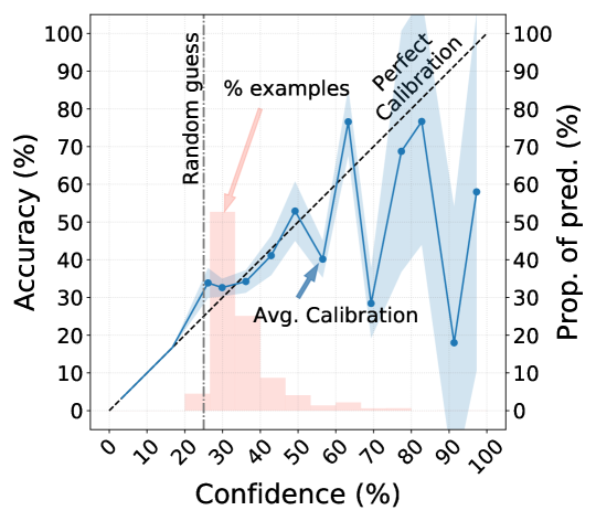
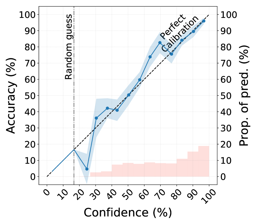
Reliability Diagram. Also called calibration curve (DeGroot & Fienberg, 1983; Niculescu-Mizil & Caruana, 2005), this is a visual representation of the calibration error, across a range of confidence values within (e.g. see Figure 1). To make this diagram, the predictions of the model are grouped in bins, according to their confidence value. For each bin , , a point is drawn where the x-axis is the average confidence of the predictions in the bin:
| while the y-axis is their average accuracy: | ||||
where is the number of examples in the -th bin and is the indicator function.
Expected Calibration Error (ECE). This metric (Naeini et al., 2015; Guo et al., 2017) is a single number that summarizes the calibration error. ECE is the average of the gaps in the reliability diagram, weighted by the number of predictions in each bin, computed as
| ECE |
where is the number of bins and the total number of examples. ECE, however, can be small for models that make mostly random predictions regardless of the calibration of examples with high confidence, since random predictions tend to be calibrated. The model in Figure 1 has a low ECE (4.29%) while decision-makers —that care about making better-than-odds predictions— would likely consider it an unreliable model. In a better-than-odds prediction, being in the predicted class is more likely than not being in the predicted class. To address this shortcoming of ECE, we propose : an ECE computed only over examples with better-than-odds confidence (higher than 50%). In the example of Figure 1, is 17.12%, which better matches the confidence someone looking for better-than-odds predictions should have in the model.
3 Miscalibration of Graph Neural Networks
In this section we investigate the calibration of successful GNNs on a selection of datasets.
| Accuracy (%) | ECE (%) | (%) | ||||||||
|---|---|---|---|---|---|---|---|---|---|---|
| Dataset | Model | Original | Random | Original | Isotonic Reg. | Temp. Scaling | Original | Hist. Binning | Isotonic Reg. | Temp. Scaling |
| Friendster | GCN-MCD | 35.09 (00.94) | 25.00 | 4.40 (01.21) | 6.43 (01.59) | 4.29 (01.37) | 17.18 (04.40) | 39.98 (00.18) | 16.46 (05.34) | 17.12 (05.02) |
| GAT | 32.40 (01.55) | 25.00 | 6.51 (01.88) | 4.13 (00.89) | 3.63 (01.69) | 35.48 (04.78) | 40.59 (00.16) | 39.13 (04.83) | 36.50 (07.71) | |
| GIN-MCD | 27.63 (01.13) | 25.00 | 3.18 (00.87) | 7.00 (01.75) | 2.71 (00.81) | 30.83 (08.44) | 40.71 (00.17) | 46.04 (02.28) | 39.83 (12.66) | |
| PubMed | GCN-MCD | 87.67 (00.50) | 33.33 | 4.12 (00.45) | 1.43 (00.38) | 1.12 (00.24) | 4.05 (00.42) | 2.08 (00.43) | 1.39 (00.37) | 1.04 (00.23) |
| GAT-MCD | 87.03 (00.45) | 33.33 | 5.07 (00.36) | 2.01 (00.27) | 1.64 (00.28) | 5.14 (00.37) | 1.76 (00.26) | 1.99 (00.26) | 1.57 (00.32) | |
| GIN | 86.66 (00.42) | 33.33 | 4.66 (00.37) | 1.74 (00.31) | 1.68 (00.36) | 4.62 (00.32) | 1.80 (00.50) | 1.69 (00.26) | 1.56 (00.34) | |
| CiteSeer | GCN-MCD | 74.90 (01.32) | 16.67 | 23.53 (01.29) | 6.45 (01.49) | 5.22 (01.06) | 24.23 (02.12) | 5.46 (01.62) | 5.59 (01.64) | 5.27 (01.18) |
| GAT | 73.57 (01.62) | 16.67 | 29.85 (01.64) | 7.45 (01.43) | 6.82 (01.75) | 28.55 (01.80) | 5.91 (01.43) | 7.16 (01.62) | 5.53 (01.33) | |
| GIN-MCD | 62.88 (01.24) | 16.67 | 5.67 (01.51) | 6.92 (01.31) | 5.95 (01.19) | 5.43 (01.62) | 5.52 (01.70) | 6.06 (01.99) | 6.55 (01.93) | |
w/o calibrating
w/ Temp. Scaling
w/ Temp. Scaling
w/ Temp. Scaling
Datasets and GNN models.
We train GNNs for the task of node classification in the following graphs: Friendster111https://github.com/PurdueMINDS/GNNsMiscalibrated (social network); CiteSeer, PubMed (Sen et al., 2008) (citation networks). Detailed description, as well as results for other graphs (Cora, Amazon and Facebook) can be found in the Supplementary Material.
We train the following GNNs: Graph Convolutional Networks (GCN) (Kipf & Welling, 2017), Graph Attention Networks (GAT) (Veličković et al., 2018) and Graph Isomorphism Network (GIN) (Xu et al., 2019). Our implementation uses the PyTorch-Geometric library (Fey & Lenssen, 2019). More details on hyperparameter search and optimization procedure in the Supplementary Material.
Existing calibration methods.
After training the GNNs, we apply techniques commonly used to improve the uncertainty quantification and the calibration of the model. These include MC Dropout (Gal & Ghahramani, 2016), Histogram Binning (Zadrozny & Elkan, 2001), Isotonic Regression (Zadrozny & Elkan, 2002) and Temperature Scaling (Guo et al., 2017). More details of these methods and our experimental setup can be found in the Supplementary Material.
Calibrating for balanced classes.
In many datasets, it is common to face an imbalanced class distribution, which can pose challenges to learn meaningful models. In our Friendster dataset, we observe a severe class imbalance, with the one class having 60% of the nodes, while another class has less than 1% of the nodes, which led to collapsed predictions towards a single (most prevalent) class, with all GNNs predicting at least 95% of examples to a single class (or, in some cases, even predicting 100% examples in a single class). To overcome this, we force the class distribution to be balanced during the training, by weighting the loss function —i.e., upweighting the examples of the less prevalent classes— such that all examples contribute equally.
When the test and train distribution are different, conclusions drawn from the evaluation can be misleading. Thus, in our case of a balanced-class loss function in training, it is paramount to evaluate the model with balanced class distributions in testing, by applying the same weighting scheme when computing the test metrics (Accuracy and ECE). As the results in Table 1 show, using the proper test distribution when evaluating has an impact on both accuracy and calibration. In particular, for our hardest task (Friendster), we see that evaluating under a test distribution similar to that used for training has an impact on ECE greater than that of calibrating the trained model. More details and results for other dataset can be found in the Supplementary Material.
Results.
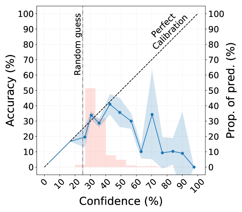
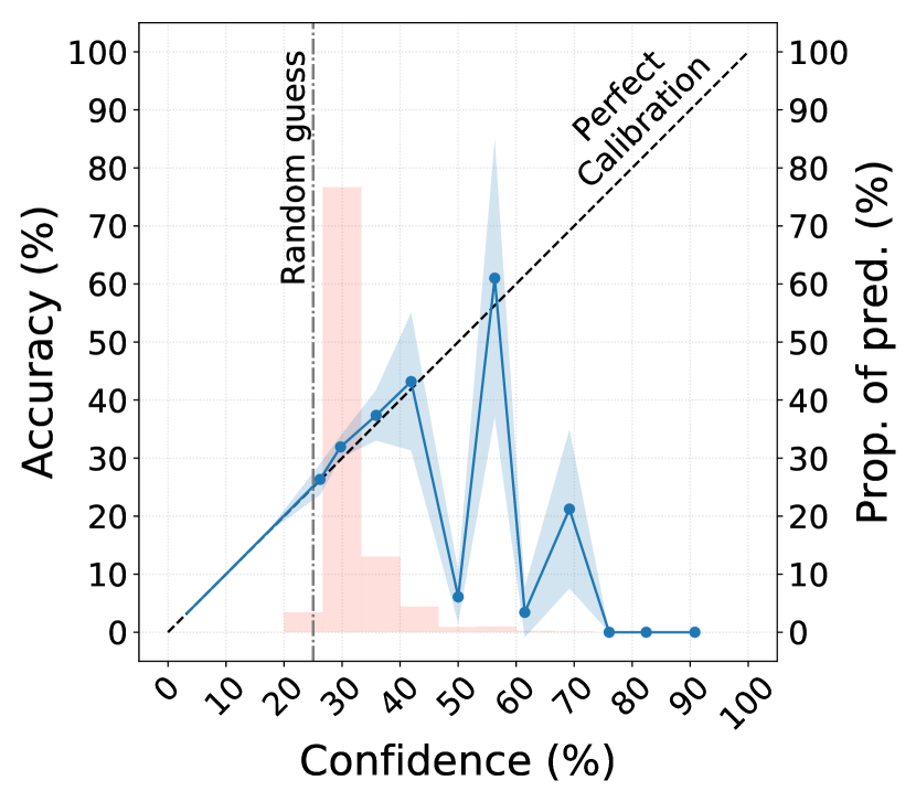
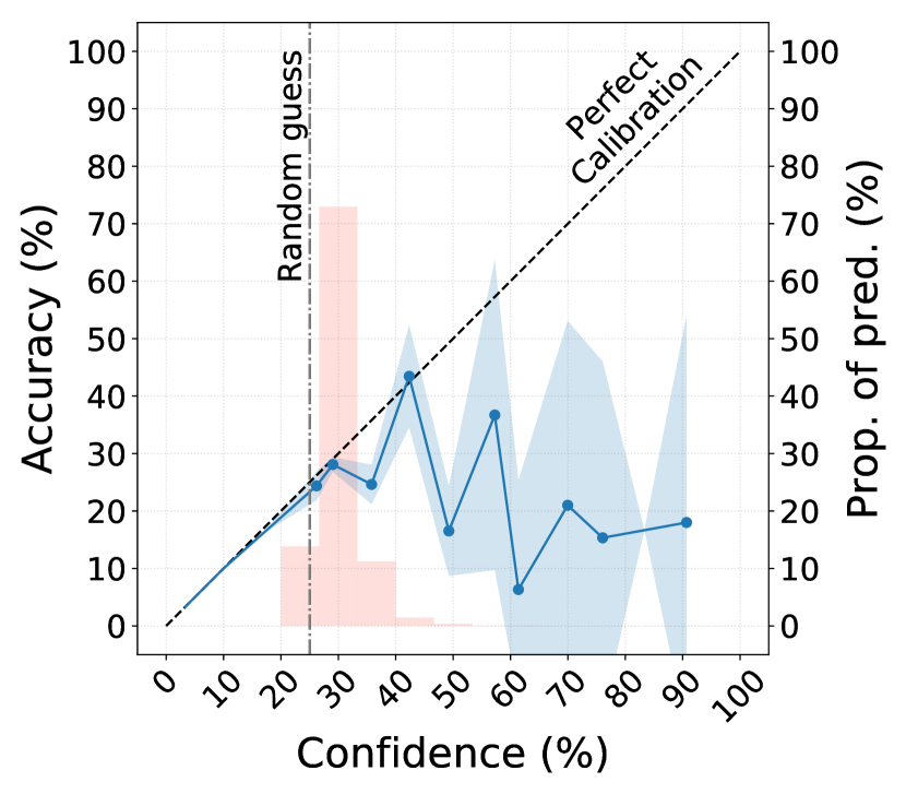
In Table 2 we present the results for the GNNs applied to Friendster —our hardest task— as well as for two common benchmark datasets. For tasks other than Friendster, existing methods are capable of improving calibration, with temperature scaling usually giving the best results. However, we also see that for harder tasks (Friendster), none of the existing calibration methods we tried were enough to fix it, particularly failing at the less frequent (but overconfident) predictions. Moreover, we see that ECE does not capture miscalibration of such predictions, which might be essential for high-stakes decision making, while the proposed presents itself as a useful metric.
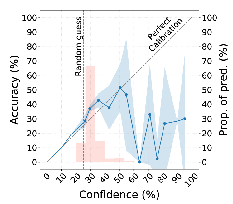
As an example, we see that the ECE for GIN with MC-Dropout on Friendster, with Temperature Scaling, is less than half of the value of ECE for GCN with MC-Dropout and Temperature Scaling for CiteSeer, indicating a better calibrated model, while from a visual inspection of the reliability diagrams (Figures 2(c) and 2(d)) we would make the opposite conclusion. The metric captures the miscalibration that is apparent in the diagrams.
The diagrams in Figure 2 also show an important aspect of ECE: while applying Temperature Scaling to the GAT model in Friendster produces a model with lower ECE, the calibration of the more confident predictions actually gets worse (Figures 2(a) and 2(b)). As the Temperature Scaling method minimizes the negative log-likelihood, the region of close-to-random predictions (which has a larger fraction of examples) has higher impact on the loss (and ECE). What we observe is that those predictions become calibrated (which brings the ECE down), at the expense of making the calibration of the less frequent predictions (confidence above 50%) worse, as those examples have a smaller impact in the loss. In this case, the proposed captures that those predictions remain miscalibrated.
4 Conclusion
In this work we empirically investigate the calibration of Graph Neural Networks (GNNs). Our results show that for easier tasks all GNNs are reasonably calibrated, while for harder tasks, such as our Friendster dataset, GNNs can be miscalibrated and existing calibration techniques are unable to calibrate them. We also propose a new ECE-derived calibration metric. Our results show the need to develop new methods to improve GNN calibration to increase their trustworthiness in high-stakes decision-making.
Acknowledgements
This work was sponsored in part by the ARO, under the U.S. Army Research Laboratory contract number W911NF-09-2-0053, the Purdue Integrative Data Science Initiative and the Purdue Research foundation, the DOD through SERC under contract number HQ0034-13-D-0004RT #206, and the National Science Foundation under contract numbers IIS-1816499 and DMS-1812197.
References
- Battaglia et al. (2018) Battaglia, P. W., Hamrick, J. B., Bapst, V., Sanchez-Gonzalez, A., Zambaldi, V., Malinowski, M., Tacchetti, A., Raposo, D., Santoro, A., Faulkner, R., Gulcehre, C., Song, F., Ballard, A., Gilmer, J., Dahl, G., Vaswani, A., Allen, K., Nash, C., Langston, V., Dyer, C., Heess, N., Wierstra, D., Kohli, P., Botvinick, M., Vinyals, O., Li, Y., and Pascanu, R. Relational inductive biases, deep learning, and graph networks. arXiv:1806.01261 [cs, stat], 2018. URL http://arxiv.org/abs/1806.01261.
- Blattenberger & Lad (1985) Blattenberger, G. and Lad, F. Separating the Brier Score into Calibration and Refinement Components: A Graphical Exposition. The American Statistician, 39(1):26–32, February 1985. ISSN 0003-1305. doi: 10.1080/00031305.1985.10479382.
- Box (1980) Box, G. E. Sampling and bayes’ inference in scientific modelling and robustness. Journal of the Royal Statistical Society: Series A (General), 143(4):383–404, 1980.
- Brier (1950) Brier, G. W. Verification of forecasts expressed in terms of probability. Monthly Weather Review, 78(1):1–3, January 1950. ISSN 0027-0644. doi: 10.1175/1520-0493(1950)078<0001:VOFEIT>2.0.CO;2.
- Card et al. (2019) Card, D., Zhang, M., and Smith, N. A. Deep Weighted Averaging Classifiers. In Proceedings of the Conference on Fairness, Accountability, and Transparency, pp. 369–378, New York, NY, USA, 2019. ACM. ISBN 978-1-4503-6125-5. doi: 10.1145/3287560.3287595.
- DeGroot & Fienberg (1983) DeGroot, M. H. and Fienberg, S. E. The Comparison and Evaluation of Forecasters. Journal of the Royal Statistical Society. Series D (The Statistician), 32(1/2):12–22, 1983. ISSN 0039-0526. doi: 10.2307/2987588.
- Duvenaud et al. (2015) Duvenaud, D. K., Maclaurin, D., Iparraguirre, J., Bombarell, R., Hirzel, T., Aspuru-Guzik, A., and Adams, R. P. Convolutional Networks on Graphs for Learning Molecular Fingerprints. In Cortes, C., Lawrence, N. D., Lee, D. D., Sugiyama, M., and Garnett, R. (eds.), Advances in Neural Information Processing Systems 28, pp. 2224–2232. Curran Associates, Inc., 2015.
- Fey & Lenssen (2019) Fey, M. and Lenssen, J. E. Fast graph representation learning with PyTorch Geometric. In ICLR Workshop on Representation Learning on Graphs and Manifolds, 2019.
- Gal & Ghahramani (2016) Gal, Y. and Ghahramani, Z. Dropout as a Bayesian Approximation: Representing Model Uncertainty in Deep Learning. In Proceedings of The 33rd International Conference on Machine Learning, PMLR, volume 48, pp. 1050–1059, New York, NY, USA, June 2016. JMLR.org.
- Gao et al. (2017) Gao, Y., Parameswaran, A., and Peng, J. On the Interpretability of Conditional Probability Estimates in the Agnostic Setting. In Artificial Intelligence and Statistics, pp. 1367–1374, April 2017.
- Gilmer et al. (2017) Gilmer, J., Schoenholz, S. S., Riley, P. F., Vinyals, O., and Dahl, G. E. Neural Message Passing for Quantum Chemistry. In International Conference on Machine Learning, pp. 1263–1272, July 2017.
- Guo et al. (2017) Guo, C., Pleiss, G., Sun, Y., and Weinberger, K. Q. On Calibration of Modern Neural Networks. In International Conference on Machine Learning, pp. 1321–1330, July 2017.
- Ioffe & Szegedy (2015) Ioffe, S. and Szegedy, C. Batch Normalization: Accelerating Deep Network Training by Reducing Internal Covariate Shift. In International Conference on Machine Learning, pp. 448–456, June 2015.
- Jones et al. (2001–) Jones, E., Oliphant, T., Peterson, P., et al. SciPy: Open source scientific tools for Python, 2001–. URL http://www.scipy.org/. [Online; accessed <today>].
- Kingma & Ba (2014) Kingma, D. P. and Ba, J. Adam: A Method for Stochastic Optimization. In International Conference on Learning Representations, 2014.
- Kipf & Welling (2017) Kipf, T. N. and Welling, M. Semi-Supervised Classification with Graph Convolutional Networks. In International Conference on Learning Representations, 2017.
- Kuleshov et al. (2018) Kuleshov, V., Fenner, N., and Ermon, S. Accurate Uncertainties for Deep Learning Using Calibrated Regression. In International Conference on Machine Learning, pp. 2796–2804, July 2018.
- Kumar et al. (2018) Kumar, A., Sarawagi, S., and Jain, U. Trainable Calibration Measures for Neural Networks from Kernel Mean Embeddings. In International Conference on Machine Learning, pp. 2805–2814, July 2018.
- Laakso & Taagepera (1979) Laakso, M. and Taagepera, R. “effective” number of parties: a measure with application to west europe. Comparative political studies, 12(1):3–27, 1979.
- Lakshminarayanan et al. (2017) Lakshminarayanan, B., Pritzel, A., and Blundell, C. Simple and Scalable Predictive Uncertainty Estimation using Deep Ensembles. In Guyon, I., Luxburg, U. V., Bengio, S., Wallach, H., Fergus, R., Vishwanathan, S., and Garnett, R. (eds.), Advances in Neural Information Processing Systems 30, pp. 6402–6413. Curran Associates, Inc., 2017.
- Leskovec & Faloutsos (2006) Leskovec, J. and Faloutsos, C. Sampling from large graphs. In Proceedings of the 12th ACM SIGKDD International Conference on Knowledge Discovery and Data Mining, pp. 631–636, 2006.
- Linderman et al. (2019) Linderman, G. C., Rachh, M., Hoskins, J. G., Steinerberger, S., and Kluger, Y. Fast interpolation-based t-SNE for improved visualization of single-cell RNA-seq data. Nature Methods, 16(3):243, March 2019. ISSN 1548-7105. doi: 10.1038/s41592-018-0308-4.
- Maaten & Hinton (2008) Maaten, L. v. d. and Hinton, G. Visualizing data using t-sne. Journal of machine learning research, 9(Nov):2579–2605, 2008.
- Mozafari et al. (2018) Mozafari, A. S., Gomes, H. S., Janny, S., and Gagné, C. A New Loss Function for Temperature Scaling to have Better Calibrated Deep Networks. In NeurIPS - Workshop on Security in Machine Learning, October 2018.
- Murphy et al. (2019) Murphy, R. L., Srinivasan, B., Rao, V., and Ribeiro, B. Janossy pooling: Learning deep permutation-invariant functions for variable-size inputs. In ICLR, 2019.
- Naeini et al. (2015) Naeini, M. P., Cooper, G. F., and Hauskrecht, M. Obtaining Well Calibrated Probabilities Using Bayesian Binning. In Proceedings of the 29th AAAI Conference on Artificial Intelligence, volume 2015, pp. 2901–2907, January 2015.
- Nair & Hinton (2010) Nair, V. and Hinton, G. E. Rectified linear units improve restricted boltzmann machines. In Proceedings of the 27th international conference on machine learning (ICML-10), pp. 807–814, 2010.
- Niculescu-Mizil & Caruana (2005) Niculescu-Mizil, A. and Caruana, R. Predicting Good Probabilities with Supervised Learning. In International Conference on Machine Learning (ICML), pp. 625–632, New York, NY, USA, 2005. ISBN 978-1-59593-180-1. doi: 10.1145/1102351.1102430.
- Pedregosa et al. (2011) Pedregosa, F., Varoquaux, G., Gramfort, A., Michel, V., Thirion, B., Grisel, O., Blondel, M., Prettenhofer, P., Weiss, R., Dubourg, V., Vanderplas, J., Passos, A., Cournapeau, D., Brucher, M., Perrot, M., and Duchesnay, E. Scikit-learn: Machine learning in Python. Journal of Machine Learning Research, 12:2825–2830, 2011.
- Platt (1999) Platt, J. Probabilistic outputs for support vector machines and comparisons to regularized likelihood methods. Advances in large margin classifiers, 10(3):61–74, 1999.
- Raposo et al. (2017) Raposo, D., Santoro, A., Barrett, D., Pascanu, R., Lillicrap, T., and Battaglia, P. Discovering objects and their relations from entangled scene representations. In Workshops at the International Conference on Learning Representations (ICLR), 2017.
- Rubin et al. (1984) Rubin, D. B. et al. Bayesianly justifiable and relevant frequency calculations for the applied statistician. The Annals of Statistics, 12(4):1151–1172, 1984.
- Sanchez-Gonzalez et al. (2018) Sanchez-Gonzalez, A., Heess, N., Springenberg, J. T., Merel, J., Riedmiller, M., Hadsell, R., and Battaglia, P. Graph Networks as Learnable Physics Engines for Inference and Control. In Dy, J. and Krause, A. (eds.), Proceedings of the 35th International Conference on Machine Learning, volume 80, pp. 4470–4479. PMLR, July 2018.
- Satorras & Estrach (2018) Satorras, V. G. and Estrach, J. B. Few-Shot Learning with Graph Neural Networks. In International Conference on Learning Representations, 2018.
- Sen et al. (2008) Sen, P., Namata, G., Bilgic, M., Getoor, L., Galligher, B., and Eliassi-Rad, T. Collective Classification in Network Data. AI Magazine, 29(3):93, 2008. ISSN 2371-9621. doi: 10.1609/aimag.v29i3.2157.
- Shchur et al. (2018) Shchur, O., Mumme, M., Bojchevski, A., and Günnemann, S. Pitfalls of Graph Neural Network Evaluation. arXiv:1811.05868 [cs, stat], November 2018.
- Simpson (1949) Simpson, E. H. Measurement of diversity. Nature, 163(4148):688, 1949.
- Sukhbaatar et al. (2016) Sukhbaatar, S., Szlam, A., and Fergus, R. Learning Multiagent Communication with Backpropagation. In Lee, D. D., Sugiyama, M., Luxburg, U. V., Guyon, I., and Garnett, R. (eds.), Advances in Neural Information Processing Systems 29, pp. 2244–2252. Curran Associates, Inc., 2016.
- Vaicenavicius et al. (2019) Vaicenavicius, J., Widmann, D., Andersson, C., Lindsten, F., Roll, J., and Schön, T. B. Evaluating model calibration in classification. In International Conference on Artificial Intelligence and Statistics (AISTATS), Naha, Okinawa, Japan, 2019.
- Veličković et al. (2018) Veličković, P., Cucurull, G., Casanova, A., Romero, A., Liò, P., and Bengio, Y. Graph Attention Networks. In International Conference on Learning Representations, Vancouver, Canada, 2018.
- Xu et al. (2019) Xu, K., Hu, W., Leskovec, J., and Jegelka, S. How Powerful are Graph Neural Networks? In International Conference on Learning Representations, 2019.
- Yang et al. (2017) Yang, J., Ribeiro, B., and Neville, J. Stochastic Gradient Descent for Relational Logistic Regression via Partial Network Crawls. In Proceedings of The 7th International International Workshop on Statistical Relational AI (StarAI), July 2017.
- Zadrozny & Elkan (2001) Zadrozny, B. and Elkan, C. Obtaining Calibrated Probability Estimates from Decision Trees and Naive Bayesian Classifiers. In Proceedings of the Eighteenth International Conference on Machine Learning, ICML ’01, pp. 609–616, San Francisco, CA, USA, 2001. Morgan Kaufmann Publishers Inc. ISBN 978-1-55860-778-1.
- Zadrozny & Elkan (2002) Zadrozny, B. and Elkan, C. Transforming Classifier Scores into Accurate Multiclass Probability Estimates. In Proceedings of the Eighth ACM SIGKDD International Conference on Knowledge Discovery and Data Mining, pp. 694–699, Edmonton, Alberta, Canada, 2002. ACM. ISBN 1-58113-567-X. doi: 10.1145/775047.775151.
Appendix A Datasets and GNN models
In this section we give more detailed information on the datasets and models we used.
A.1 Datasets
The datasets we used are composed of citation networks, social networks and co-purchased goods. For all datasets, we randomly split the labeled nodes into three sets: training, validation and test, in the proportions described in Table 3. A brief description of each dataset is given in the following paragraphs.
Friendster:
social network, where nodes represent users and edges represent friendship relationships. The features of the nodes include numerical features (e.g age, number of photos posted, etc) and categorical features (e.g. gender, college, music interests, etc), encoded as binary one-hot features, for a total of 644 features. As an extra pre-processing step, we standardize all the features to have mean 0 and variance 1, across all nodes. The predicted label is the relationship status of the user, which can be one of four values: Single, Married, In A Relationship or Domestic Partner. There are also nodes without label, which we use when computing the embeddings, but are outside of the set of labeled nodes we use to train (compute the loss) and evaluate the model. The full graph has a largest connected component of more than 6 million nodes. However, due to the challenges of training GNNs on large graphs of this size, we obtained a sample of the larger graph, using the Forest Fire procedure (Leskovec & Faloutsos, 2006). This smaller version of the graph contain 40K nodes, 25K of which are labeled.
Facebook (Yang et al., 2017):
social network of Facebook users from Purdue university, where nodes represent users and edges represent friendship relationships. The feature of the nodes are: religious views, sex and whether the user’s hometown is in Indiana. In addition to those features, we also add the degree of the nodes, as one-hot encoding, bringing the total number of features to 85. As an extra pre-processing step, we standardize all the features to have mean 0 and variance 1, across all nodes. The predicted label is the political view. The graph used is a subset of the entire graph used in Yang et al. (2017), composed by all the users who represented all the features.
Cora, CiteSeer, PubMed (Sen et al., 2008):
citation networks, where the nodes represent papers and the edges represent a citation (undirected) between papers. The features of the nodes are textual features (bag-of-words). As in (Kipf & Welling, 2017), we normalize the features of each node, to have unitary norm. The predicted label is the topic of the paper. Note that, while some other works (e.g. Kipf & Welling (2017)) employ a semi-supervised setting, using only a small fraction of nodes for training, we follow a supervised setting, where all nodes are used for either training, validation or testing.
Cora-Full (Shchur et al., 2018):
an extended version of Cora, with a larger number of nodes, features and labels. As before, nodes represent papers and edges represent a (undirected) citation between papers. Node features are textual representations of the content and labels are the topic of the paper.
Amazon-Computers, Amazon-Photo (Shchur et al., 2018)
: segments of the co-purchased graph from Amazon. Nodes are goods, edges between nodes indicate they are frequently co-purchased. Features are bag-of-words encoding of reviews of the product, while labels are given by the category.
Table 3 gives detailed statistics of the datasets.
| Dataset | Classes | Features | Nodes | Edges | Edge density | Train | Validation | Test split |
|---|---|---|---|---|---|---|---|---|
| Friendster | 4 | 644 | 43880 | 145407 | 0.00015 | 15629 | 3126 | 6251 |
| 2 | 85 | 4556 | 23325 | 0.00225 | 2848 | 569 | 1139 | |
| Cora | 7 | 1433 | 2708 | 5278 | 0.00144 | 1208 | 500 | 1000 |
| CiteSeer | 6 | 3703 | 3327 | 4552 | 0.00082 | 2080 | 416 | 831 |
| PubMed | 3 | 500 | 19717 | 44324 | 0.00023 | 12324 | 2464 | 4929 |
| Cora-Full | 70 | 8710 | 19793 | 63421 | 0.00032 | 12371 | 2474 | 4948 |
| Amazon-Cmp. | 10 | 767 | 13752 | 245861 | 0.00260 | 8595 | 1719 | 3438 |
| Amazon-Ph. | 8 | 745 | 7650 | 119081 | 0.00407 | 4782 | 956 | 1912 |
A.2 GNN models
In our experiments, we employed the Graph Convolutional Networks (GCN) from Kipf & Welling (2017), Graph Attention Networks (GAT) from Veličković et al. (2018) and Graph Isomorphism Networks (GIN) from (Xu et al., 2019). The models were implemented using the PyTorch-Geometric library (Fey & Lenssen, 2019). For GIN, we learn the parameter and use a two-layer MLP with Batch Normalization (Ioffe & Szegedy, 2015) ReLU activation (Nair & Hinton, 2010) at each layer.
MC-Dropout
(Gal & Ghahramani, 2016) is a simple way of improving the uncertainty estimations of a model with Dropout, by doing multiple forward passes, sampling a different dropout mask each time and averaging the results (instead of the mean approximation of using a single forward pass, without dropping neurons but multiplying them by the dropout rate). While a useful (and simple) way of improving the conditional probability estimated by the model, this procedure does not targeted at enforcing a calibrated model, and a calibration method can be applied on top of it, to improve the model calibration. In our experiments, we use 100 forward passes when applying MC Dropout. We use the suffix “-MCD” to denote when we apply MC Dropout with 100 forward passes to the trained GNN.
A.3 Calibration Methods
For the calibration methods, we employed three procedures which have been previously applied in the literature, which we describe here. Similarly to what was done in Guo et al. (2017), for Histogram Binning and Isotonic Regression, we train one version of the model for each class in a one-vs-all manner, which means that after the calibration, the estimated probabilities for one example need not sum to one across all classes and the predicted class might change, based on the transformed confidence values for each class (although we observed that this happen with very low frequency).
Histogram Binning
(Zadrozny & Elkan, 2001) is a simple method which groups the predictions into bins, according to their confidence values (similar to what is done for ECE and the reliability diagrams). Then we build a mapping from the confidence range of each bin to the accuracy of the predictions of that bin, so that when a new prediction is made, we need only to see which bin it originally falls into and replace the confidence with the accuracy of that bin. In our experiments we use 15 bins.
Isotonic Regression
(Zadrozny & Elkan, 2002) can be seen as a more general version of Histogram Binning, where the number of bins and their limits are jointly learned with the piece-wise (isotonic) regression on the accuracy. As with histogram binning, we fit one model for each class in one-vs-all encoding. We use the Isotonic Regression implementation available in the scikit-learn Python package (Pedregosa et al., 2011).
Temperature Scaling
(Guo et al., 2017) is a simple extension of Platt scaling (Platt, 1999) to a multi-class setting, proposed by Guo et al. (2017). A single scalar temperature parameter is learned. This temperature parameter () scales the logit (pre-softmax) values, which will alter the estimated probabilities, without changing the predicted class. In their original paper, Guo et al. (2017) learn this parameter by optimizing the negative log-likelihood on validation data. We tested using both the negative log-likelihood as well as the Brier Score (Brier, 1950) which is a proper scoring rule that can be decomposed into a calibration and refinement term (Blattenberger & Lad, 1985). We implement it using the optimization routines from SciPy (Jones et al., 2001–).
| Dataset | Imbalance Ratio | ||||
|---|---|---|---|---|---|
| Entropy | Simpson | ||||
| Eff. Num. | Index | ||||
| Num. Classes | |||||
| Friendster | 91.62 | 1.20 | 0.35 ( 1.38 ) | 2.9 | 4 |
| Cora | 4.54 | 1.83 | 0.18 ( 1.26 ) | 5.6 | 7 |
| PubMed | 1.92 | 1.06 | 0.36 ( 1.07 ) | 2.8 | 3 |
| CiteSeer | 2.82 | 1.75 | 0.18 ( 1.07 ) | 5.6 | 6 |
| Cora-Full | 61.87 | 4.00 | 0.02 ( 1.52 ) | 46.1 | 70 |
| 1.91 | 0.64 | 0.55 ( 1.10 ) | 1.8 | 2 | |
| Amazon-Cmp. | 17.73 | 1.87 | 0.21 ( 2.08 ) | 4.8 | 10 |
| Amazon-Ph. | 5.86 | 1.93 | 0.16 ( 1.26 ) | 6.1 | 8 |
Appendix B Experimental setup and hyperparameters
For all GNNs, we tested 2, 3, and 4 layers. The number of neurons in the hidden layers was chosen from for GCN and GIN, for GAT (with 8 heads at each layer which are concatenated for intermediary layers and average for last layer, as in the original paper). For all models we used Dropout in the final fully connected layers, with the probability of zeroing a neuron chosen from . The strength of weight decay was chosen from . For GIN, we learn the parameter . We trained all models to minimize the negative log-likelihood of the training data using full-batch gradient descent and the Adam optimizer (Kingma & Ba, 2014) with learning rate chosen from and default values of betas ( and ). We trained our models for 200 epochs, stopping early if the validation performance does not improve after 50 consecutive epochs. We also decay the learning rate by a factor of 2 after each 75 epochs.
For each GNN family, we select the best model (hyperparameters) as the one which achieves best performance in the validation data. We tested using either accuracy or loss as the performance metric for early stopping and model selection. As this choice does not seem to have too much impact on the calibration of the model, we decided to use accuracy for final results presented in the paper, as this choice yields models with slightly better accuracy. In Appendix C we also present results using the validation loss as the metric for model selection and early stopping, for comparison. All models were trained using a NVidia Titan V GPU, in a host with 2.00GHz Intel(R) Xeon(R) CPU E5-2660 v4 processor and 256 GiB of RAM.
After training and selecting the best model for each GNN family, we evaluate the model (accuracy and calibration) on the test data. We compare using MC Dropout (MCD suffix on the tables) or just the regular dropout. For the evaluation, we perform 10 bootstraps of the test data and present our results as the mean and standard deviation over the bootstrap samples.
Since the calibration methods we employ are very simple and do not have hyperparameters to tune, we use the validation data to train them. After training them, we evaluate them on the test data, using the same procedure described before. For both the ECE metric and the Reliability Diagrams, we use 15 bins, which is the same number of bins used by Guo et al. (2017). We also use the same number of bins for histogram binning.
Appendix C Results

C.1 Need for balancing test distribution for Friendster
The class distribution in our Friendster dataset is severely imbalanced. The unlabeled nodes constitute 43% of the nodes in the graph (while not used to compute the loss or the evaluation, they are used in the neighborhood of other nodes when computing their embeddings). Of the remaining 25K labeled nodes, 66.5% belong to the class Single, 14.3 % to the class Married, 18.4 % to the class In A Relationship and 0.8 % to the class Domestic Partner.
This severe class imbalance leads to challenges during the training, such as collapsing the predictions towards the most prevalent class. In our experiments, when training the GNNs without weighting the loss, all three models heavily biases their predictions towards the prevalent class, with GCN predicting 95.5% of the test nodes as Single, GAT predicting 96.2%, and GIN 98.7%. For some configurations of hyperparameters, we even observed that the GNNs predicted all test nodes as Single (we see this for all three GNNs). These models achieve around 66% accuracy in the test, which is the proportion of Single nodes in the test data.
If we want our models to learn something more useful than just predicting any node as Single, we need to deal with the class imbalance. A common way of remedying this issue is to weight the loss function, such that each example contributes the same towards the loss, regardless of its class. With this approach, we are adding and extra assumption to our model, that the distribution of the class labels is balanced.
It is important, however, to maintain this assumption when evaluating our models as well. If we balance the classes only during training, but keep the test data unbalanced, we are evaluating our model under a distribution different from that for which it was trained. To avoid facing the challenges incurred by this type of domain adaptation, we must also evaluate our model with a balanced distribution, which can also be achieved by simply weighting the evaluation metrics in such a way that every example contributes the same, regardless of its class.
In Section A.3 we present measurements of diversity of the distribution of class labels on each dataset. We compute: (1) the ratio between the size of the largest class and the size of the smallest class; (2) entropy, as , where is the proportion of examples in class ; (3) Simpson’s index (Simpson, 1949), given by , which can be interpreted as the probability that two uniformly and independently sampled examples come from the same class, as well as how much larger this index is than if it was computed in a balanced dataset; (4) Effective Number of Classes (Laakso & Taagepera, 1979), given by the inverse of Simpson’s index. As can be seen in the table, while Friendster has the most extreme imbalance when comparing the largest and smallest classes, other datasets also present some level of class imbalance. Faced with these challenges, we decided for balancing the classes in all of our models, even for the other datasets, where the class imbalance is less severe. We also employ the same balancing strategy when training the calibration methods and computing our evaluation metrics.
For the sake of comparison, we present here in the Supplementary Material the results when the model was trained with balanced classes but evaluated with imbalanced classes as well. While the full results are presented in the next section, we also show a summary in Table 5, comparing the accuracy and ECE under both scenarios. One interesting observation is how in some cases, such as for our harder Friendster dataset, simply evaluating under the balanced distribution (by weighting the metrics), as it was trained for, had a greater impact in ECE than applying a calibration method such as Temperature Scaling, but still evaluating under an imbalanced test distribution.
| w/o Balancing | w/ Balancing | ||||||
|---|---|---|---|---|---|---|---|
| Accuracy (%) | ECE (%) | Accuracy (%) | ECE (%) | ||||
| Dataset | Model | Original | Original | Temp. Scaling | Original | Original | Temp. Scaling |
| Friendster | GCN | 39.70 (00.56) | 10.40 (00.78) | 10.90 (00.49) | 35.08 (02.32) | 4.08 (01.13) | 4.32 (01.27) |
| GCN-MCD | 40.48 (00.69) | 11.04 (00.74) | 11.02 (00.64) | 35.09 (00.94) | 4.40 (01.21) | 4.29 (01.37) | |
| GAT | 29.03 (00.40) | 9.39 (00.37) | 5.97 (00.39) | 32.40 (01.55) | 6.51 (01.88) | 3.63 (01.69) | |
| GAT-MCD | 28.53 (00.59) | 8.23 (00.54) | 5.22 (00.53) | 31.24 (01.63) | 5.60 (01.64) | 3.56 (01.43) | |
| GIN | 23.84 (00.54) | 7.90 (00.45) | 7.68 (00.58) | 26.74 (00.84) | 3.43 (00.79) | 3.66 (00.64) | |
| GIN-MCD | 23.91 (00.45) | 8.26 (00.33) | 7.81 (00.42) | 27.63 (01.13) | 3.18 (00.87) | 2.71 (00.81) | |
| GCN | 69.07 (01.49) | 4.93 (00.84) | 4.88 (01.50) | 70.15 (01.44) | 6.16 (01.55) | 5.49 (00.87) | |
| GCN-MCD | 71.44 (00.91) | 6.98 (00.84) | 4.67 (01.41) | 69.49 (01.08) | 5.31 (00.80) | 4.55 (01.08) | |
| GAT | 67.45 (01.64) | 5.58 (01.72) | 4.21 (01.10) | 67.19 (02.08) | 5.92 (01.57) | 4.02 (00.76) | |
| GAT-MCD | 68.47 (01.27) | 5.94 (00.41) | 6.23 (00.98) | 68.62 (01.23) | 6.28 (00.93) | 5.75 (01.26) | |
| GIN | 66.11 (01.97) | 5.81 (01.87) | 4.45 (00.89) | 65.11 (01.24) | 5.61 (00.79) | 5.65 (01.48) | |
| GIN-MCD | 65.56 (01.58) | 4.18 (01.16) | 4.76 (00.98) | 65.64 (01.68) | 4.78 (00.98) | 5.48 (01.58) | |
| Cora | GCN | 86.03 (01.25) | 4.76 (01.07) | 4.56 (01.00) | 86.00 (01.25) | 5.31 (01.08) | 5.53 (01.05) |
| GCN-MCD | 86.06 (00.56) | 10.87 (00.64) | 4.23 (00.69) | 86.00 (01.02) | 10.23 (00.80) | 4.69 (00.79) | |
| GAT | 85.29 (00.88) | 47.81 (00.80) | 4.30 (00.55) | 86.31 (01.07) | 48.01 (01.00) | 4.56 (00.88) | |
| GAT-MCD | 84.79 (01.01) | 47.15 (00.85) | 4.68 (00.79) | 85.30 (01.07) | 46.96 (01.22) | 5.01 (00.76) | |
| GIN | 83.35 (01.14) | 9.65 (01.17) | 5.75 (00.99) | 84.61 (00.80) | 8.76 (00.72) | 6.03 (01.20) | |
| GIN-MCD | 83.77 (00.85) | 3.81 (00.62) | 4.90 (01.36) | 83.44 (01.49) | 5.18 (00.77) | 5.28 (01.21) | |
| CiteSeer | GCN | 77.21 (01.05) | 19.71 (00.92) | 5.56 (01.45) | 74.39 (01.76) | 17.71 (01.79) | 5.30 (00.85) |
| GCN-MCD | 77.32 (01.48) | 25.27 (01.10) | 4.47 (01.12) | 74.90 (01.32) | 23.53 (01.29) | 5.84 (01.14) | |
| GAT | 75.99 (01.11) | 30.68 (01.13) | 5.69 (00.87) | 73.57 (01.62) | 29.85 (01.64) | 7.11 (01.14) | |
| GAT-MCD | 76.49 (01.22) | 31.85 (01.23) | 6.86 (01.00) | 72.05 (01.82) | 29.37 (01.91) | 5.84 (01.38) | |
| GIN | 67.00 (00.83) | 8.38 (00.77) | 6.07 (00.70) | 62.85 (01.70) | 11.75 (01.57) | 6.90 (01.24) | |
| GIN-MCD | 66.87 (01.47) | 7.63 (01.22) | 7.46 (01.44) | 62.88 (01.24) | 5.67 (01.51) | 6.28 (00.56) | |
| PubMed | GCN | 87.31 (00.57) | 1.53 (00.34) | 1.31 (00.37) | 87.63 (00.42) | 1.77 (00.30) | 1.25 (00.21) |
| GCN-MCD | 87.51 (00.48) | 4.07 (00.36) | 1.38 (00.46) | 87.67 (00.50) | 4.12 (00.45) | 1.35 (00.20) | |
| GAT | 86.71 (00.35) | 3.25 (00.37) | 1.50 (00.26) | 86.92 (00.50) | 3.42 (00.49) | 1.62 (00.26) | |
| GAT-MCD | 86.53 (00.25) | 4.85 (00.27) | 1.25 (00.32) | 87.03 (00.45) | 5.07 (00.36) | 1.64 (00.28) | |
| GIN | 86.93 (00.40) | 4.66 (00.41) | 1.79 (00.34) | 86.66 (00.42) | 4.66 (00.37) | 1.68 (00.36) | |
| GIN-MCD | 86.84 (00.21) | 3.53 (00.26) | 1.86 (00.29) | 86.30 (00.59) | 3.85 (00.36) | 2.21 (00.26) | |
| Amazon-Cmp. | GCN | 87.97 (00.57) | 5.29 (00.52) | 2.90 (00.51) | 91.51 (00.54) | 3.77 (00.36) | 1.98 (00.48) |
| GCN-MCD | 88.18 (00.47) | 5.56 (00.48) | 2.65 (00.47) | 91.51 (00.60) | 3.76 (00.59) | 1.81 (00.45) | |
| GAT | 91.03 (00.48) | 2.15 (00.41) | 2.17 (00.32) | 93.15 (00.46) | 1.80 (00.33) | 1.94 (00.44) | |
| GAT-MCD | 90.84 (00.43) | 2.03 (00.40) | 2.58 (00.43) | 93.20 (00.26) | 2.26 (00.41) | 1.68 (00.35) | |
| GIN | 88.66 (00.45) | 3.69 (00.58) | 3.67 (00.50) | 92.11 (00.53) | 2.85 (00.37) | 2.35 (00.44) | |
| GIN-MCD | 88.66 (00.42) | 7.86 (00.43) | 2.61 (00.29) | 92.08 (00.53) | 7.28 (00.46) | 2.27 (00.61) | |
| Amazon-Ph. | GCN | 93.06 (00.36) | 1.50 (00.34) | 1.92 (00.49) | 93.61 (00.69) | 1.71 (00.32) | 2.23 (00.44) |
| GCN-MCD | 93.47 (00.37) | 1.74 (00.28) | 1.73 (00.23) | 93.68 (00.86) | 1.74 (00.34) | 2.19 (00.37) | |
| GAT | 93.41 (00.60) | 2.84 (00.58) | 1.67 (00.42) | 93.38 (00.77) | 3.13 (00.53) | 2.20 (00.51) | |
| GAT-MCD | 93.11 (00.49) | 2.44 (00.42) | 1.89 (00.25) | 93.04 (00.47) | 2.54 (00.33) | 1.90 (00.39) | |
| GIN | 92.51 (00.63) | 2.89 (00.83) | 2.51 (00.45) | 93.96 (00.59) | 2.74 (00.36) | 2.72 (00.63) | |
| GIN-MCD | 92.68 (00.53) | 2.32 (00.33) | 2.27 (00.41) | 93.87 (00.61) | 2.49 (00.55) | 2.74 (00.56) | |
C.2 Misclassification on Friendster
Among the datasets we tested, Friendster is the hardest task. While for other tasks we achieve more than 90% accuracy, all models tested on Friendster achieve accuracy levels closer to that of random predictions.
In Figure 3 we plot the nodes of the three datasets with largest ratio between largest and smallest class. The positions are computed from the node’s features, using a Fast Fourier Transform-accelerated Interpolation-based implementation of t-SNE (Linderman et al., 2019; Maaten & Hinton, 2008). The colors are the true labels.
As can be seen in the figure, for datasets other than Friendster, the features of the nodes have sufficient signal to produce a reasonable embedding of the nodes, while for Friendster, the embedding based on the features alone carries no information about the classes. This could indicate that, for other tasks, the features of the nodes have a stronger signal when compared with the Friendster dataset.
We also investigated the examples misclassified for the GCN model on Friendster and found that the nodes with label “In A Relationship” have the highest misclassification rate (93% misclassified). Of the misclassified examples of this class, 47.3 % are assigned the label “Single” and 46.4 % are assigned as either “Domestic Partner” (14.1 %) or “Married” (32.3%). Further investigation on why the performance is so poor on Friendster is left as future work.
C.3 Calibration Results
In Tables 6, 7, 8 and 9 we present the ECE results for all GNNs in all datasets, with and without balancing the metrics to correct for class imbalance, using accuracy or loss for early stopping / model selection. The results for the same models are present in the corresponding Tables 10, 11, 12 and 13.
We also investigate the calibration of a Logistic Regression model (with L1 regularization) for Friendster. This model obtains accuracy levels similar to GCN with MC Dropout, but still miscalibrated. In Figure 4 we present the reliability diagram, after applying Temperature Scaling. Even when applying a non-i.i.d. model, the state-of-the-art calibration method is not capable of solving the problem, which reinforces the need to develop calibration methods that take into account the non-i.i.d. nature of the data as well.
| Early Stopping and Model Selection using: Balanced Validation Accuracy, Test Metrics: Not Balanced | ||||||||
|---|---|---|---|---|---|---|---|---|
| Accuracy (%) | ECE (%) | |||||||
| Dataset | Model | Original | Random | Original | Hist. Bin. | Isotonic | TS w/ NLL | TS w/ Brier |
| Friendster | GCN | 39.70 (00.56) | 25.00 | 10.40 (00.78) | 3.79 (00.47) | 6.69 (00.80) | 10.90 (00.49) | 10.68 (00.79) |
| GCN-MCD | 40.48 (00.69) | 25.00 | 11.04 (00.74) | 4.67 (00.55) | 8.84 (00.52) | 11.02 (00.64) | 10.98 (00.44) | |
| GAT | 29.03 (00.40) | 25.00 | 9.39 (00.37) | 2.73 (00.45) | 15.22 (00.50) | 5.97 (00.39) | 6.89 (00.62) | |
| GAT-MCD | 28.53 (00.59) | 25.00 | 8.23 (00.54) | 3.29 (00.69) | 17.05 (00.62) | 5.22 (00.53) | 6.39 (00.43) | |
| GIN | 23.84 (00.54) | 25.00 | 7.90 (00.45) | 1.31 (00.60) | 10.70 (00.58) | 7.68 (00.58) | 8.02 (00.66) | |
| GIN-MCD | 23.91 (00.45) | 25.00 | 8.26 (00.33) | 1.40 (00.44) | 8.54 (00.56) | 7.81 (00.42) | 7.99 (00.56) | |
| Cora | GCN | 86.03 (01.25) | 14.29 | 4.76 (01.07) | 5.87 (00.92) | 6.99 (00.83) | 4.56 (01.00) | 6.51 (00.90) |
| GCN-MCD | 86.06 (00.56) | 14.29 | 10.87 (00.64) | 4.93 (00.49) | 5.22 (01.19) | 4.23 (00.69) | 5.19 (00.91) | |
| GAT | 85.29 (00.88) | 14.29 | 47.81 (00.80) | 6.19 (01.26) | 3.75 (01.09) | 4.30 (00.55) | 4.17 (00.93) | |
| GAT-MCD | 84.79 (01.01) | 14.29 | 47.15 (00.85) | 4.18 (01.00) | 3.20 (00.73) | 4.68 (00.79) | 5.01 (00.84) | |
| GIN | 83.35 (01.14) | 14.29 | 9.65 (01.17) | 5.80 (01.26) | 5.55 (01.05) | 5.75 (00.99) | 6.55 (01.25) | |
| GIN-MCD | 83.77 (00.85) | 14.29 | 3.81 (00.62) | 6.32 (00.97) | 5.21 (00.76) | 4.90 (01.36) | 4.53 (00.82) | |
| PubMed | GCN | 87.31 (00.57) | 33.33 | 1.53 (00.34) | 1.63 (00.36) | 1.90 (00.34) | 1.31 (00.37) | 1.20 (00.35) |
| GCN-MCD | 87.51 (00.48) | 33.33 | 4.07 (00.36) | 2.01 (00.22) | 1.87 (00.26) | 1.38 (00.46) | 1.38 (00.48) | |
| GAT | 86.71 (00.35) | 33.33 | 3.25 (00.37) | 1.69 (00.41) | 1.49 (00.25) | 1.50 (00.26) | 1.41 (00.30) | |
| GAT-MCD | 86.53 (00.25) | 33.33 | 4.85 (00.27) | 1.61 (00.26) | 1.76 (00.34) | 1.25 (00.32) | 1.42 (00.22) | |
| GIN | 86.93 (00.40) | 33.33 | 4.66 (00.41) | 1.61 (00.44) | 1.80 (00.22) | 1.79 (00.34) | 1.71 (00.34) | |
| GIN-MCD | 86.84 (00.21) | 33.33 | 3.53 (00.26) | 1.45 (00.31) | 2.33 (00.34) | 1.86 (00.29) | 2.29 (00.26) | |
| CiteSeer | GCN | 77.21 (01.05) | 16.67 | 19.71 (00.92) | 4.67 (01.33) | 5.09 (01.13) | 5.56 (01.45) | 5.92 (01.01) |
| GCN-MCD | 77.32 (01.48) | 16.67 | 25.27 (01.10) | 4.45 (00.84) | 5.22 (00.76) | 4.47 (01.12) | 4.65 (00.90) | |
| GAT | 75.99 (01.11) | 16.67 | 30.68 (01.13) | 5.46 (00.91) | 7.42 (01.20) | 5.69 (00.87) | 5.16 (00.75) | |
| GAT-MCD | 76.49 (01.22) | 16.67 | 31.85 (01.23) | 6.29 (00.69) | 4.74 (00.53) | 6.86 (01.00) | 5.60 (01.30) | |
| GIN | 67.00 (00.83) | 16.67 | 8.38 (00.77) | 5.99 (01.11) | 6.08 (00.78) | 6.07 (00.70) | 7.23 (01.29) | |
| GIN-MCD | 66.87 (01.47) | 16.67 | 7.63 (01.22) | 5.93 (01.36) | 7.46 (00.99) | 7.46 (01.44) | 7.01 (01.40) | |
| Cora-Full | GCN | 70.34 (00.61) | 1.43 | 5.79 (00.59) | 5.98 (00.61) | 5.68 (00.43) | 5.46 (00.54) | 4.99 (00.31) |
| GCN-MCD | 70.31 (00.55) | 1.43 | 6.83 (00.41) | 4.25 (00.47) | 3.62 (00.46) | 3.78 (00.47) | 3.49 (00.56) | |
| GAT | 69.44 (00.51) | 1.43 | 3.58 (00.48) | 4.63 (00.41) | 4.26 (00.37) | 4.36 (00.59) | 3.73 (00.49) | |
| GAT-MCD | 69.90 (00.54) | 1.43 | 3.48 (00.54) | 4.00 (00.32) | 3.94 (00.40) | 3.59 (00.75) | 3.21 (00.35) | |
| GIN | 68.84 (00.45) | 1.43 | 13.48 (00.75) | 5.43 (00.62) | 5.20 (00.44) | 11.32 (00.42) | 9.41 (00.20) | |
| GIN-MCD | 68.94 (00.77) | 1.43 | 31.76 (00.60) | 5.77 (00.55) | 3.46 (00.49) | 6.56 (00.43) | 6.13 (00.74) | |
| GCN | 69.07 (01.49) | 50.00 | 4.93 (00.84) | 5.21 (01.01) | 9.81 (01.31) | 4.88 (01.50) | 5.15 (01.08) | |
| GCN-MCD | 71.44 (00.91) | 50.00 | 6.98 (00.84) | 5.59 (00.70) | 8.67 (00.95) | 4.67 (01.41) | 5.20 (00.95) | |
| GAT | 67.45 (01.64) | 50.00 | 5.58 (01.72) | 5.36 (00.91) | 17.37 (00.73) | 4.21 (01.10) | 4.75 (00.94) | |
| GAT-MCD | 68.47 (01.27) | 50.00 | 5.94 (00.41) | 6.31 (01.42) | 11.83 (01.35) | 6.23 (00.98) | 5.27 (01.12) | |
| GIN | 66.11 (01.97) | 50.00 | 5.81 (01.87) | 3.73 (01.02) | 8.92 (01.02) | 4.45 (00.89) | 5.52 (01.26) | |
| GIN-MCD | 65.56 (01.58) | 50.00 | 4.18 (01.16) | 4.84 (00.85) | 8.10 (01.71) | 4.76 (00.98) | 4.98 (01.13) | |
| Amazon-Cmp. | GCN | 87.97 (00.57) | 10.00 | 5.29 (00.52) | 1.78 (00.41) | 3.76 (00.24) | 2.90 (00.51) | 3.49 (00.50) |
| GCN-MCD | 88.18 (00.47) | 10.00 | 5.56 (00.48) | 2.80 (00.26) | 3.51 (00.55) | 2.65 (00.47) | 3.43 (00.58) | |
| GAT | 91.03 (00.48) | 10.00 | 2.15 (00.41) | 2.28 (00.31) | 3.73 (00.45) | 2.17 (00.32) | 3.10 (00.33) | |
| GAT-MCD | 90.84 (00.43) | 10.00 | 2.03 (00.40) | 2.21 (00.38) | 3.33 (00.45) | 2.58 (00.43) | 3.15 (00.44) | |
| GIN | 88.66 (00.45) | 10.00 | 3.69 (00.58) | 1.91 (00.35) | 4.26 (00.46) | 3.67 (00.50) | 4.04 (00.41) | |
| GIN-MCD | 88.66 (00.42) | 10.00 | 7.86 (00.43) | 2.01 (00.47) | 4.06 (00.37) | 2.61 (00.29) | 3.16 (00.53) | |
| Amazon-Ph. | GCN | 93.06 (00.36) | 12.50 | 1.50 (00.34) | 1.95 (00.56) | 2.29 (00.47) | 1.92 (00.49) | 1.75 (00.47) |
| GCN-MCD | 93.47 (00.37) | 12.50 | 1.74 (00.28) | 1.59 (00.29) | 2.41 (00.43) | 1.73 (00.23) | 1.95 (00.61) | |
| GAT | 93.41 (00.60) | 12.50 | 2.84 (00.58) | 1.71 (00.39) | 2.34 (00.42) | 1.67 (00.42) | 1.70 (00.22) | |
| GAT-MCD | 93.11 (00.49) | 12.50 | 2.44 (00.42) | 1.90 (00.31) | 2.55 (00.49) | 1.89 (00.25) | 2.69 (00.54) | |
| GIN | 92.51 (00.63) | 12.50 | 2.89 (00.83) | 1.86 (00.56) | 2.34 (00.34) | 2.51 (00.45) | 3.24 (00.42) | |
| GIN-MCD | 92.68 (00.53) | 12.50 | 2.32 (00.33) | 2.39 (00.33) | 2.35 (00.49) | 2.27 (00.41) | 2.69 (00.43) | |
| Early Stopping using: Validation Accuracy, Test Metrics: Balanced | ||||||||
|---|---|---|---|---|---|---|---|---|
| Accuracy (%) | ECE (%) | |||||||
| Dataset | Model | Original | Random | Original | Hist. Bin. | Isotonic | TS w/ NLL | TS w/ Brier |
| Friendster | GCN | 35.08 (02.32) | 25.00 | 4.08 (01.13) | 39.48 (00.24) | 5.70 (01.66) | 4.32 (01.27) | 4.87 (00.90) |
| GCN-MCD | 35.09 (00.94) | 25.00 | 4.40 (01.21) | 39.57 (00.17) | 6.43 (01.59) | 4.29 (01.37) | 5.20 (01.42) | |
| GAT | 32.40 (01.55) | 25.00 | 6.51 (01.88) | 40.54 (00.16) | 4.13 (00.89) | 3.63 (01.69) | 4.28 (01.19) | |
| GAT-MCD | 31.24 (01.63) | 25.00 | 5.60 (01.64) | 40.66 (00.14) | 3.99 (00.66) | 3.56 (01.43) | 4.32 (01.13) | |
| GIN | 26.74 (00.84) | 25.00 | 3.43 (00.79) | 40.72 (00.08) | 7.44 (00.76) | 3.66 (00.64) | 4.50 (01.15) | |
| GIN-MCD | 27.63 (01.13) | 25.00 | 3.18 (00.87) | 40.69 (00.16) | 7.00 (01.75) | 2.71 (00.81) | 2.88 (01.05) | |
| Cora | GCN | 86.00 (01.25) | 14.29 | 5.31 (01.08) | 6.51 (00.86) | 6.66 (01.27) | 5.53 (01.05) | 5.57 (00.95) |
| GCN-MCD | 86.00 (01.02) | 14.29 | 10.23 (00.80) | 5.22 (01.20) | 4.88 (00.67) | 4.69 (00.79) | 5.14 (01.08) | |
| GAT | 86.31 (01.07) | 14.29 | 48.01 (01.00) | 5.72 (00.78) | 3.55 (00.62) | 4.56 (00.88) | 4.90 (00.65) | |
| GAT-MCD | 85.30 (01.07) | 14.29 | 46.96 (01.22) | 4.35 (00.79) | 3.58 (00.70) | 5.01 (00.76) | 4.79 (00.92) | |
| GIN | 84.61 (00.80) | 14.29 | 8.76 (00.72) | 5.12 (01.10) | 5.71 (00.67) | 6.03 (01.20) | 6.90 (00.94) | |
| GIN-MCD | 83.44 (01.49) | 14.29 | 5.18 (00.77) | 7.73 (01.16) | 5.54 (01.53) | 5.28 (01.21) | 5.51 (00.90) | |
| PubMed | GCN | 87.63 (00.42) | 33.33 | 1.77 (00.30) | 1.85 (00.27) | 1.51 (00.34) | 1.25 (00.21) | 1.25 (00.21) |
| GCN-MCD | 87.67 (00.50) | 33.33 | 4.12 (00.45) | 2.06 (00.47) | 1.43 (00.38) | 1.35 (00.20) | 1.12 (00.24) | |
| GAT | 86.92 (00.50) | 33.33 | 3.42 (00.49) | 2.06 (00.32) | 1.87 (00.26) | 1.62 (00.26) | 1.64 (00.47) | |
| GAT-MCD | 87.03 (00.45) | 33.33 | 5.07 (00.36) | 2.01 (00.31) | 2.01 (00.27) | 1.64 (00.28) | 1.75 (00.40) | |
| GIN | 86.66 (00.42) | 33.33 | 4.66 (00.37) | 1.97 (00.48) | 1.74 (00.31) | 1.68 (00.36) | 1.83 (00.33) | |
| GIN-MCD | 86.30 (00.59) | 33.33 | 3.85 (00.36) | 2.00 (00.35) | 1.83 (00.50) | 2.21 (00.26) | 2.21 (00.32) | |
| CiteSeer | GCN | 74.39 (01.76) | 16.67 | 17.71 (01.79) | 4.48 (01.02) | 5.56 (01.11) | 5.30 (00.85) | 5.81 (00.93) |
| GCN-MCD | 74.90 (01.32) | 16.67 | 23.53 (01.29) | 6.55 (01.26) | 6.45 (01.49) | 5.84 (01.14) | 5.22 (01.06) | |
| GAT | 73.57 (01.62) | 16.67 | 29.85 (01.64) | 6.35 (01.85) | 7.45 (01.43) | 7.11 (01.14) | 6.82 (01.75) | |
| GAT-MCD | 72.05 (01.82) | 16.67 | 29.37 (01.91) | 5.82 (01.45) | 6.06 (01.20) | 5.84 (01.38) | 6.83 (00.67) | |
| GIN | 62.85 (01.70) | 16.67 | 11.75 (01.57) | 5.41 (00.94) | 6.05 (01.05) | 6.90 (01.24) | 6.49 (01.48) | |
| GIN-MCD | 62.88 (01.24) | 16.67 | 5.67 (01.51) | 6.24 (01.14) | 6.92 (01.31) | 6.28 (00.56) | 5.95 (01.19) | |
| Cora-Full | GCN | 69.62 (00.87) | 1.43 | 6.73 (00.98) | 7.82 (01.06) | 6.96 (00.52) | 5.18 (00.56) | 5.37 (00.94) |
| GCN-MCD | 69.49 (00.91) | 1.43 | 6.07 (00.49) | 7.61 (00.63) | 5.24 (00.66) | 4.15 (00.83) | 3.46 (00.71) | |
| GAT | 68.81 (01.17) | 1.43 | 4.62 (00.58) | 7.55 (00.70) | 5.88 (00.73) | 4.34 (00.73) | 4.34 (00.65) | |
| GAT-MCD | 69.39 (00.91) | 1.43 | 3.95 (00.50) | 6.49 (00.82) | 5.52 (00.68) | 4.17 (00.48) | 3.61 (00.53) | |
| GIN | 66.71 (00.63) | 1.43 | 11.01 (01.01) | 6.90 (00.91) | 6.02 (00.37) | 9.69 (00.86) | 9.48 (00.53) | |
| GIN-MCD | 65.84 (01.14) | 1.43 | 27.62 (00.92) | 5.80 (00.46) | 3.07 (00.61) | 6.25 (00.81) | 6.28 (00.69) | |
| GCN | 70.15 (01.44) | 50.00 | 6.16 (01.55) | 12.59 (01.03) | 7.55 (00.86) | 5.49 (00.87) | 5.64 (01.13) | |
| GCN-MCD | 69.49 (01.08) | 50.00 | 5.31 (00.80) | 12.95 (01.18) | 5.73 (01.42) | 4.55 (01.08) | 5.50 (01.01) | |
| GAT | 67.19 (02.08) | 50.00 | 5.92 (01.57) | 15.99 (00.91) | 6.78 (01.09) | 4.02 (00.76) | 4.82 (01.07) | |
| GAT-MCD | 68.62 (01.23) | 50.00 | 6.28 (00.93) | 8.92 (01.13) | 6.39 (01.04) | 5.75 (01.26) | 5.35 (01.15) | |
| GIN | 65.11 (01.24) | 50.00 | 5.61 (00.79) | 11.85 (02.08) | 6.14 (01.26) | 5.65 (01.48) | 5.64 (01.83) | |
| GIN-MCD | 65.64 (01.68) | 50.00 | 4.78 (00.98) | 11.88 (01.57) | 6.37 (00.81) | 5.48 (01.58) | 6.21 (01.70) | |
| Amazon-Cmp. | GCN | 91.51 (00.54) | 10.00 | 3.77 (00.36) | 2.83 (00.36) | 2.74 (00.41) | 1.98 (00.48) | 2.17 (00.40) |
| GCN-MCD | 91.51 (00.60) | 10.00 | 3.76 (00.59) | 2.07 (00.54) | 2.33 (00.60) | 1.81 (00.45) | 2.25 (00.29) | |
| GAT | 93.15 (00.46) | 10.00 | 1.80 (00.33) | 2.45 (00.64) | 2.43 (00.28) | 1.94 (00.44) | 2.73 (00.47) | |
| GAT-MCD | 93.20 (00.26) | 10.00 | 2.26 (00.41) | 1.99 (00.34) | 2.25 (00.36) | 1.68 (00.35) | 2.79 (00.43) | |
| GIN | 92.11 (00.53) | 10.00 | 2.85 (00.37) | 4.18 (00.52) | 2.47 (00.34) | 2.35 (00.44) | 2.71 (00.50) | |
| GIN-MCD | 92.08 (00.53) | 10.00 | 7.28 (00.46) | 3.52 (00.53) | 2.68 (00.39) | 2.27 (00.61) | 2.38 (00.35) | |
| Amazon-Ph. | GCN | 93.61 (00.69) | 12.50 | 1.71 (00.32) | 2.37 (00.27) | 2.33 (00.35) | 2.23 (00.44) | 1.70 (00.46) |
| GCN-MCD | 93.68 (00.86) | 12.50 | 1.74 (00.34) | 2.17 (00.59) | 2.27 (00.51) | 2.19 (00.37) | 1.69 (00.31) | |
| GAT | 93.38 (00.77) | 12.50 | 3.13 (00.53) | 1.79 (00.32) | 2.09 (00.31) | 2.20 (00.51) | 1.84 (00.39) | |
| GAT-MCD | 93.04 (00.47) | 12.50 | 2.54 (00.33) | 2.28 (00.44) | 2.28 (00.55) | 1.90 (00.39) | 2.10 (00.39) | |
| GIN | 93.96 (00.59) | 12.50 | 2.74 (00.36) | 2.33 (00.35) | 2.41 (00.42) | 2.72 (00.63) | 2.86 (00.57) | |
| GIN-MCD | 93.87 (00.61) | 12.50 | 2.49 (00.55) | 2.73 (00.28) | 2.24 (00.50) | 2.74 (00.56) | 2.94 (00.67) | |
| Early Stopping using: Validation Loss, Test Metrics: Not Balanced | ||||||||
|---|---|---|---|---|---|---|---|---|
| Accuracy (%) | ECE (%) | |||||||
| Dataset | Model | Original | Random | Original | Hist. Bin. | Isotonic | TS w/ NLL | TS w/ Brier |
| Friendster | GCN | 31.97 (00.60) | 25.00 | 6.26 (00.72) | 3.27 (00.51) | 12.10 (00.43) | 7.06 (00.33) | 7.26 (00.40) |
| GCN-MCD | 31.17 (00.34) | 25.00 | 4.95 (00.44) | 3.13 (00.64) | 15.22 (00.52) | 6.77 (00.44) | 6.38 (00.43) | |
| GAT | 24.67 (00.61) | 25.00 | 7.39 (00.66) | 2.03 (00.31) | 17.94 (00.61) | 5.80 (00.37) | 6.03 (00.74) | |
| GAT-MCD | 27.83 (00.51) | 25.00 | 4.42 (00.42) | 1.77 (00.36) | 10.87 (00.49) | 3.81 (00.30) | 3.91 (00.46) | |
| GIN | 23.75 (00.39) | 25.00 | 8.00 (00.38) | 1.39 (00.47) | 11.06 (00.52) | 7.99 (00.53) | 8.26 (00.51) | |
| GIN-MCD | 24.23 (00.58) | 25.00 | 7.87 (00.66) | 1.31 (00.70) | 15.57 (00.57) | 8.06 (00.31) | 7.71 (00.58) | |
| Cora | GCN | 86.19 (01.12) | 14.29 | 5.19 (00.75) | 5.87 (01.17) | 6.67 (01.08) | 5.08 (00.87) | 5.72 (00.83) |
| GCN-MCD | 85.30 (00.90) | 14.29 | 10.19 (01.03) | 4.83 (00.78) | 5.58 (00.57) | 4.03 (00.75) | 4.49 (00.95) | |
| GAT | 85.46 (01.14) | 14.29 | 4.26 (00.77) | 4.98 (01.07) | 5.66 (00.78) | 4.99 (00.58) | 3.98 (01.02) | |
| GAT-MCD | 84.81 (01.01) | 14.29 | 3.92 (00.47) | 6.15 (01.43) | 6.00 (01.23) | 4.87 (00.89) | 4.18 (00.93) | |
| GIN | 83.64 (00.72) | 14.29 | 6.11 (01.01) | 6.03 (00.89) | 5.61 (00.97) | 6.12 (01.25) | 5.57 (00.60) | |
| GIN-MCD | 84.14 (01.63) | 14.29 | 6.58 (00.72) | 5.25 (01.04) | 5.50 (00.96) | 6.11 (00.60) | 6.46 (01.19) | |
| PubMed | GCN | 87.96 (00.45) | 33.33 | 1.85 (00.39) | 1.58 (00.40) | 1.35 (00.22) | 1.72 (00.28) | 1.76 (00.31) |
| GCN-MCD | 87.98 (00.35) | 33.33 | 3.38 (00.43) | 1.50 (00.20) | 1.63 (00.47) | 1.43 (00.20) | 1.58 (00.35) | |
| GAT | 87.71 (00.49) | 33.33 | 2.02 (00.39) | 2.30 (00.41) | 1.73 (00.37) | 1.69 (00.56) | 1.37 (00.38) | |
| GAT-MCD | 87.93 (00.57) | 33.33 | 1.53 (00.29) | 1.94 (00.32) | 1.95 (00.21) | 1.65 (00.36) | 1.44 (00.29) | |
| GIN | 87.31 (00.69) | 33.33 | 1.36 (00.29) | 1.55 (00.28) | 1.76 (00.42) | 1.35 (00.40) | 1.19 (00.17) | |
| GIN-MCD | 87.23 (00.43) | 33.33 | 1.39 (00.20) | 1.65 (00.25) | 1.71 (00.36) | 1.26 (00.26) | 1.61 (00.27) | |
| CiteSeer | GCN | 76.92 (01.15) | 16.67 | 5.10 (01.20) | 5.12 (00.84) | 5.41 (01.12) | 4.37 (01.06) | 5.03 (01.11) |
| GCN-MCD | 77.57 (01.06) | 16.67 | 12.25 (00.99) | 4.80 (01.01) | 5.57 (00.69) | 4.41 (01.07) | 5.02 (00.88) | |
| GAT | 75.50 (01.46) | 16.67 | 9.60 (01.21) | 4.80 (00.92) | 6.12 (01.24) | 4.64 (00.80) | 4.41 (00.72) | |
| GAT-MCD | 74.66 (01.67) | 16.67 | 9.97 (01.15) | 4.25 (01.30) | 5.98 (00.93) | 3.82 (00.79) | 4.20 (00.70) | |
| GIN | 69.24 (01.42) | 16.67 | 6.89 (01.35) | 6.30 (01.03) | 6.76 (01.23) | 6.87 (01.23) | 6.36 (00.84) | |
| GIN-MCD | 68.86 (01.47) | 16.67 | 6.76 (01.48) | 5.64 (01.11) | 6.02 (01.04) | 6.56 (01.08) | 6.85 (00.78) | |
| Cora-Full | GCN | 69.87 (00.61) | 1.43 | 4.45 (00.29) | 5.47 (00.67) | 4.91 (00.63) | 4.68 (00.50) | 4.31 (00.27) |
| GCN-MCD | 69.93 (00.74) | 1.43 | 14.91 (00.57) | 2.93 (00.32) | 2.88 (00.41) | 3.48 (00.44) | 3.28 (00.52) | |
| GAT | 69.67 (00.46) | 1.43 | 3.78 (00.28) | 4.56 (00.48) | 4.21 (00.38) | 4.43 (00.43) | 4.02 (00.35) | |
| GAT-MCD | 69.14 (00.72) | 1.43 | 3.04 (00.72) | 4.49 (00.53) | 4.14 (00.50) | 3.02 (00.53) | 3.17 (00.59) | |
| GIN | 63.50 (00.85) | 1.43 | 4.62 (00.79) | 5.29 (00.50) | 3.84 (00.53) | 7.28 (00.42) | 3.83 (00.59) | |
| GIN-MCD | 63.30 (00.60) | 1.43 | 19.35 (00.65) | 4.81 (00.73) | 3.70 (00.58) | 3.99 (00.59) | 2.59 (00.56) | |
| GCN | 68.87 (01.38) | 50.00 | 5.88 (01.18) | 6.31 (01.47) | 9.20 (01.26) | 6.01 (00.95) | 4.94 (01.03) | |
| GCN-MCD | 69.30 (01.27) | 50.00 | 6.37 (01.15) | 5.51 (01.04) | 8.16 (00.75) | 5.99 (00.83) | 5.86 (00.80) | |
| GAT | 65.02 (01.83) | 50.00 | 4.43 (01.03) | 4.55 (01.04) | 7.68 (01.38) | 4.29 (01.17) | 4.19 (01.04) | |
| GAT-MCD | 67.07 (01.81) | 50.00 | 5.39 (01.15) | 2.98 (01.02) | 7.56 (01.36) | 4.57 (01.02) | 3.79 (00.83) | |
| GIN | 66.33 (01.93) | 50.00 | 4.83 (01.87) | 3.98 (00.97) | 8.85 (00.90) | 4.40 (00.91) | 4.51 (01.11) | |
| GIN-MCD | 66.06 (01.91) | 50.00 | 3.77 (00.95) | 3.40 (00.96) | 9.67 (01.27) | 4.60 (00.80) | 5.01 (00.97) | |
| Amazon-Cmp. | GCN | 87.59 (00.65) | 10.00 | 4.33 (00.59) | 1.81 (00.36) | 4.05 (00.47) | 2.80 (00.39) | 3.33 (00.41) |
| GCN-MCD | 87.80 (00.30) | 10.00 | 4.62 (00.43) | 2.08 (00.34) | 3.90 (00.65) | 2.38 (00.50) | 3.38 (00.48) | |
| GAT | 89.42 (00.52) | 10.00 | 1.95 (00.50) | 2.09 (00.39) | 4.07 (00.40) | 2.34 (00.43) | 2.18 (00.43) | |
| GAT-MCD | 89.63 (00.64) | 10.00 | 1.63 (00.52) | 2.19 (00.37) | 3.51 (00.69) | 2.18 (00.57) | 1.87 (00.30) | |
| GIN | 89.28 (00.68) | 10.00 | 3.72 (00.54) | 1.74 (00.41) | 4.44 (00.43) | 3.59 (00.27) | 3.60 (00.44) | |
| GIN-MCD | 89.17 (00.65) | 10.00 | 3.65 (00.46) | 1.90 (00.26) | 4.49 (00.41) | 3.54 (00.44) | 3.46 (00.19) | |
| Amazon-Ph. | GCN | 93.36 (00.61) | 12.50 | 2.21 (00.41) | 2.03 (00.29) | 2.18 (00.51) | 2.23 (00.46) | 2.25 (00.53) |
| GCN-MCD | 93.01 (00.69) | 12.50 | 2.13 (00.31) | 1.74 (00.35) | 1.81 (00.29) | 2.21 (00.52) | 2.17 (00.57) | |
| GAT | 93.27 (00.57) | 12.50 | 1.67 (00.23) | 2.01 (00.63) | 1.76 (00.39) | 1.71 (00.31) | 1.90 (00.49) | |
| GAT-MCD | 93.38 (00.46) | 12.50 | 2.07 (00.37) | 2.13 (00.48) | 1.72 (00.25) | 1.78 (00.32) | 1.88 (00.26) | |
| GIN | 92.53 (00.75) | 12.50 | 3.36 (00.72) | 2.69 (00.65) | 2.92 (00.51) | 2.40 (00.30) | 3.68 (00.49) | |
| GIN-MCD | 92.20 (00.52) | 12.50 | 1.97 (00.26) | 2.17 (00.57) | 2.78 (00.47) | 2.25 (00.41) | 2.82 (00.43) | |
| Early Stopping using: Validation Loss, Test Metrics: Balanced | ||||||||
|---|---|---|---|---|---|---|---|---|
| Accuracy (%) | ECE (%) | |||||||
| Dataset | Model | Original | Random | Original | Hist. Bin. | Isotonic | TS w/ NLL | TS w/ Brier |
| Friendster | GCN | 35.11 (01.35) | 25.00 | 7.03 (01.61) | 39.81 (00.24) | 4.78 (01.50) | 5.11 (01.35) | 5.88 (01.37) |
| GCN-MCD | 33.31 (01.21) | 25.00 | 4.16 (01.01) | 39.60 (00.14) | 5.47 (01.93) | 3.53 (01.33) | 3.93 (01.11) | |
| GAT | 30.71 (01.87) | 25.00 | 4.19 (01.36) | 40.29 (00.18) | 4.70 (00.82) | 4.36 (01.33) | 4.23 (01.45) | |
| GAT-MCD | 28.81 (01.44) | 25.00 | 4.20 (01.43) | 40.14 (00.16) | 5.93 (00.88) | 3.44 (01.46) | 3.67 (01.15) | |
| GIN | 26.82 (00.91) | 25.00 | 3.17 (00.87) | 40.78 (00.14) | 7.01 (01.49) | 3.07 (00.50) | 3.83 (00.90) | |
| GIN-MCD | 26.90 (00.82) | 25.00 | 3.48 (00.74) | 40.60 (00.13) | 7.21 (01.40) | 3.30 (00.69) | 4.08 (00.71) | |
| Cora | GCN | 86.73 (01.81) | 14.29 | 4.32 (00.84) | 7.06 (01.08) | 6.84 (01.05) | 5.42 (01.11) | 5.91 (01.05) |
| GCN-MCD | 85.50 (01.10) | 14.29 | 9.91 (01.34) | 6.75 (01.21) | 6.27 (00.56) | 3.85 (00.91) | 5.07 (00.96) | |
| GAT | 84.24 (00.99) | 14.29 | 4.95 (00.55) | 6.16 (00.87) | 6.33 (00.75) | 5.60 (00.64) | 5.48 (00.91) | |
| GAT-MCD | 85.10 (01.67) | 14.29 | 4.06 (00.72) | 6.80 (00.85) | 5.36 (00.80) | 4.79 (01.03) | 4.54 (01.00) | |
| GIN | 83.76 (01.19) | 14.29 | 6.80 (01.48) | 6.78 (00.50) | 5.51 (01.03) | 6.07 (01.13) | 6.21 (01.24) | |
| GIN-MCD | 83.00 (01.00) | 14.29 | 6.32 (00.96) | 4.71 (00.99) | 4.83 (00.65) | 6.26 (01.04) | 6.71 (01.21) | |
| PubMed | GCN | 88.73 (00.57) | 33.33 | 1.83 (00.28) | 1.60 (00.35) | 1.53 (00.35) | 1.80 (00.35) | 1.65 (00.40) |
| GCN-MCD | 88.47 (00.44) | 33.33 | 3.77 (00.22) | 1.64 (00.27) | 1.48 (00.27) | 1.51 (00.30) | 1.53 (00.26) | |
| GAT | 88.19 (00.36) | 33.33 | 1.74 (00.23) | 2.22 (00.32) | 1.35 (00.30) | 1.53 (00.22) | 1.39 (00.36) | |
| GAT-MCD | 87.72 (00.38) | 33.33 | 1.49 (00.20) | 2.11 (00.38) | 1.31 (00.30) | 1.53 (00.29) | 1.27 (00.16) | |
| GIN | 87.38 (00.54) | 33.33 | 1.42 (00.37) | 2.00 (00.35) | 1.60 (00.39) | 1.25 (00.27) | 1.39 (00.32) | |
| GIN-MCD | 87.31 (00.60) | 33.33 | 1.38 (00.44) | 2.44 (00.23) | 1.54 (00.26) | 1.37 (00.42) | 1.44 (00.31) | |
| CiteSeer | GCN | 74.53 (02.07) | 16.67 | 5.57 (01.16) | 6.49 (01.63) | 6.02 (00.96) | 4.89 (01.07) | 6.12 (01.05) |
| GCN-MCD | 75.03 (02.35) | 16.67 | 11.33 (02.26) | 7.48 (01.37) | 6.59 (01.75) | 5.56 (01.16) | 5.60 (01.40) | |
| GAT | 74.72 (01.72) | 16.67 | 9.63 (01.73) | 6.77 (01.13) | 6.64 (00.99) | 5.65 (00.85) | 5.12 (00.77) | |
| GAT-MCD | 74.16 (01.64) | 16.67 | 9.60 (01.57) | 6.16 (00.84) | 6.34 (01.03) | 5.36 (01.00) | 5.55 (00.70) | |
| GIN | 69.49 (01.33) | 16.67 | 7.29 (01.65) | 5.49 (01.22) | 7.48 (01.37) | 7.07 (01.65) | 7.70 (00.87) | |
| GIN-MCD | 68.66 (01.33) | 16.67 | 7.88 (01.07) | 5.57 (01.18) | 7.54 (01.17) | 7.15 (00.98) | 6.88 (01.09) | |
| Cora-Full | GCN | 68.98 (01.05) | 1.43 | 4.25 (00.90) | 7.77 (00.72) | 6.38 (00.99) | 4.42 (00.54) | 4.21 (00.40) |
| GCN-MCD | 68.98 (00.90) | 1.43 | 13.43 (00.92) | 6.53 (00.93) | 3.32 (00.61) | 4.58 (00.54) | 4.08 (00.76) | |
| GAT | 68.85 (00.93) | 1.43 | 4.66 (00.47) | 7.83 (01.05) | 5.38 (00.70) | 4.01 (00.37) | 4.23 (00.58) | |
| GAT-MCD | 68.89 (01.24) | 1.43 | 3.80 (00.91) | 7.12 (00.74) | 5.25 (00.91) | 3.48 (00.91) | 4.08 (00.42) | |
| GIN | 62.45 (01.13) | 1.43 | 3.55 (00.87) | 6.77 (01.02) | 5.00 (00.41) | 5.27 (00.70) | 4.61 (00.54) | |
| GIN-MCD | 62.76 (00.84) | 1.43 | 17.81 (00.66) | 5.18 (00.88) | 4.80 (00.75) | 3.68 (00.54) | 3.51 (00.42) | |
| GCN | 70.08 (01.37) | 50.00 | 5.45 (01.11) | 9.79 (00.56) | 7.30 (00.94) | 5.06 (00.61) | 5.84 (01.02) | |
| GCN-MCD | 69.62 (01.80) | 50.00 | 5.62 (01.17) | 8.77 (01.14) | 6.99 (01.20) | 6.00 (01.33) | 5.87 (01.07) | |
| GAT | 66.15 (01.42) | 50.00 | 3.38 (00.85) | 8.45 (00.97) | 4.39 (01.18) | 3.68 (00.94) | 3.87 (01.43) | |
| GAT-MCD | 66.57 (01.62) | 50.00 | 4.37 (01.64) | 9.88 (01.11) | 4.12 (01.22) | 4.35 (01.13) | 4.48 (00.93) | |
| GIN | 64.93 (01.45) | 50.00 | 5.52 (01.17) | 11.09 (01.10) | 6.31 (00.84) | 4.92 (00.62) | 5.29 (01.04) | |
| GIN-MCD | 64.78 (01.34) | 50.00 | 4.46 (00.84) | 12.23 (00.73) | 6.01 (01.14) | 5.19 (01.28) | 5.03 (01.21) | |
| Amazon-Cmp. | GCN | 91.31 (00.64) | 10.00 | 3.38 (00.21) | 1.92 (00.60) | 2.51 (00.43) | 2.05 (00.29) | 2.57 (00.35) |
| GCN-MCD | 91.60 (00.49) | 10.00 | 3.83 (00.36) | 1.98 (00.58) | 2.29 (00.27) | 1.69 (00.30) | 2.44 (00.42) | |
| GAT | 92.87 (00.60) | 10.00 | 1.78 (00.42) | 2.21 (00.57) | 2.68 (00.43) | 2.32 (00.49) | 2.17 (00.59) | |
| GAT-MCD | 92.54 (00.65) | 10.00 | 1.59 (00.35) | 2.52 (00.42) | 2.65 (00.48) | 1.76 (00.24) | 1.96 (00.26) | |
| GIN | 91.10 (00.48) | 10.00 | 2.84 (00.43) | 3.08 (00.66) | 2.82 (00.60) | 2.63 (00.43) | 2.48 (00.40) | |
| GIN-MCD | 91.33 (00.71) | 10.00 | 2.63 (00.43) | 2.34 (00.35) | 2.67 (00.40) | 2.63 (00.59) | 2.86 (00.44) | |
| Amazon-Ph. | GCN | 94.24 (00.58) | 12.50 | 2.20 (00.32) | 2.44 (00.58) | 1.79 (00.30) | 2.34 (00.44) | 1.90 (00.41) |
| GCN-MCD | 94.12 (00.58) | 12.50 | 2.45 (00.26) | 2.53 (00.49) | 2.05 (00.43) | 2.36 (00.43) | 1.85 (00.40) | |
| GAT | 93.91 (00.47) | 12.50 | 1.76 (00.42) | 2.92 (00.59) | 1.78 (00.39) | 2.06 (00.32) | 2.17 (00.64) | |
| GAT-MCD | 93.33 (00.71) | 12.50 | 2.44 (00.57) | 2.82 (00.67) | 1.83 (00.63) | 2.19 (00.46) | 2.20 (00.37) | |
| GIN | 93.31 (00.79) | 12.50 | 3.06 (00.58) | 3.36 (00.71) | 3.10 (00.57) | 2.30 (00.51) | 3.19 (00.17) | |
| GIN-MCD | 93.04 (00.40) | 12.50 | 2.27 (00.48) | 3.05 (00.87) | 2.68 (00.80) | 2.51 (00.29) | 2.87 (00.46) | |
| Early Stopping using: Validation Accuracy, Test Metrics: Not Balanced | ||||||||
|---|---|---|---|---|---|---|---|---|
| Accuracy (%) | (%) | |||||||
| Dataset | Model | Original | Random | Original | Hist. Bin. | Isotonic | TS w/ NLL | TS w/ Brier |
| Friendster | GCN | 39.70 (00.56) | 25.00 | 32.55 (01.98) | 3.71 (00.46) | 37.62 (02.51) | 31.04 (04.31) | 30.69 (02.06) |
| GCN-MCD | 40.48 (00.69) | 25.00 | 26.36 (02.17) | 4.65 (00.51) | 28.71 (01.53) | 27.51 (02.62) | 28.71 (02.16) | |
| GAT | 29.03 (00.40) | 25.00 | 48.89 (02.89) | 2.68 (00.47) | 43.16 (02.13) | 49.07 (02.51) | 52.88 (01.75) | |
| GAT-MCD | 28.53 (00.59) | 25.00 | 45.76 (03.20) | 3.29 (00.69) | 42.02 (02.77) | 43.25 (03.54) | 46.95 (04.30) | |
| GIN | 23.84 (00.54) | 25.00 | 42.58 (07.37) | 1.27 (00.59) | 47.85 (01.89) | 50.24 (08.94) | 44.74 (06.77) | |
| GIN-MCD | 23.91 (00.45) | 25.00 | 46.11 (06.00) | 1.39 (00.45) | 47.62 (01.14) | 46.48 (06.67) | 48.77 (06.25) | |
| Cora | GCN | 86.03 (01.25) | 14.29 | 3.83 (01.14) | 5.74 (01.00) | 6.28 (00.74) | 4.10 (00.95) | 5.87 (00.73) |
| GCN-MCD | 86.06 (00.56) | 14.29 | 9.82 (00.59) | 4.68 (00.49) | 5.15 (01.17) | 3.70 (00.71) | 4.46 (00.84) | |
| GAT | 85.29 (00.88) | 14.29 | 40.25 (01.13) | 5.83 (01.04) | 3.15 (00.99) | 3.92 (00.73) | 3.76 (00.92) | |
| GAT-MCD | 84.79 (01.01) | 14.29 | 37.35 (01.01) | 3.80 (00.77) | 2.39 (00.68) | 4.33 (00.70) | 4.61 (00.69) | |
| GIN | 83.35 (01.14) | 14.29 | 9.33 (01.22) | 5.79 (01.36) | 5.19 (00.97) | 4.71 (01.25) | 5.52 (01.15) | |
| GIN-MCD | 83.77 (00.85) | 14.29 | 3.35 (00.65) | 5.85 (00.94) | 4.88 (00.71) | 4.32 (01.33) | 3.96 (00.90) | |
| PubMed | GCN | 87.31 (00.57) | 33.33 | 1.45 (00.33) | 1.57 (00.30) | 1.84 (00.31) | 1.21 (00.37) | 1.10 (00.35) |
| GCN-MCD | 87.51 (00.48) | 33.33 | 3.98 (00.35) | 2.03 (00.28) | 1.82 (00.27) | 1.35 (00.44) | 1.28 (00.47) | |
| GAT | 86.71 (00.35) | 33.33 | 3.18 (00.37) | 1.54 (00.37) | 1.50 (00.25) | 1.42 (00.26) | 1.34 (00.32) | |
| GAT-MCD | 86.53 (00.25) | 33.33 | 4.84 (00.30) | 1.47 (00.26) | 1.75 (00.31) | 1.18 (00.31) | 1.32 (00.20) | |
| GIN | 86.93 (00.40) | 33.33 | 4.59 (00.46) | 1.45 (00.45) | 1.74 (00.24) | 1.73 (00.36) | 1.63 (00.33) | |
| GIN-MCD | 86.84 (00.21) | 33.33 | 3.46 (00.25) | 1.30 (00.30) | 2.23 (00.36) | 1.76 (00.28) | 2.16 (00.26) | |
| CiteSeer | GCN | 77.21 (01.05) | 16.67 | 20.15 (01.13) | 4.56 (00.98) | 4.68 (01.11) | 4.43 (01.30) | 5.07 (00.92) |
| GCN-MCD | 77.32 (01.48) | 16.67 | 25.80 (01.34) | 3.42 (00.70) | 4.17 (00.94) | 3.87 (00.97) | 4.30 (01.33) | |
| GAT | 75.99 (01.11) | 16.67 | 30.14 (01.31) | 5.34 (01.13) | 6.90 (01.13) | 5.50 (00.87) | 3.68 (00.67) | |
| GAT-MCD | 76.49 (01.22) | 16.67 | 31.56 (01.52) | 5.59 (00.80) | 4.33 (00.61) | 6.25 (01.32) | 5.56 (01.32) | |
| GIN | 67.00 (00.83) | 16.67 | 8.75 (00.85) | 5.10 (00.93) | 6.84 (01.09) | 6.08 (01.18) | 7.10 (01.59) | |
| GIN-MCD | 66.87 (01.47) | 16.67 | 7.60 (01.20) | 5.62 (01.49) | 6.73 (00.78) | 7.52 (01.50) | 7.39 (01.48) | |
| Cora-Full | GCN | 70.34 (00.61) | 1.43 | 6.49 (00.59) | 5.62 (00.57) | 6.05 (00.57) | 3.99 (00.59) | 4.44 (00.47) |
| GCN-MCD | 70.31 (00.55) | 1.43 | 4.70 (00.36) | 3.83 (00.58) | 3.56 (00.52) | 3.01 (00.49) | 2.92 (00.63) | |
| GAT | 69.44 (00.51) | 1.43 | 3.02 (00.59) | 4.48 (00.62) | 4.65 (00.40) | 3.16 (00.41) | 3.02 (00.65) | |
| GAT-MCD | 69.90 (00.54) | 1.43 | 2.36 (00.74) | 3.63 (00.54) | 4.11 (00.30) | 2.54 (00.59) | 2.59 (00.33) | |
| GIN | 68.84 (00.45) | 1.43 | 6.52 (00.57) | 5.52 (00.67) | 5.48 (00.47) | 6.09 (00.27) | 6.34 (00.65) | |
| GIN-MCD | 68.94 (00.77) | 1.43 | 27.21 (00.68) | 6.85 (00.53) | 3.57 (00.45) | 3.31 (00.66) | 3.33 (00.50) | |
| GCN | 69.07 (01.49) | 50.00 | 4.93 (00.84) | 5.21 (01.01) | 9.81 (01.31) | 4.88 (01.50) | 5.15 (01.08) | |
| GCN-MCD | 71.44 (00.91) | 50.00 | 6.98 (00.84) | 5.59 (00.70) | 8.67 (00.95) | 4.67 (01.41) | 5.20 (00.95) | |
| GAT | 67.45 (01.64) | 50.00 | 5.58 (01.72) | 5.36 (00.91) | 17.37 (00.73) | 4.21 (01.10) | 4.75 (00.94) | |
| GAT-MCD | 68.47 (01.27) | 50.00 | 5.94 (00.41) | 6.31 (01.42) | 11.83 (01.35) | 6.23 (00.98) | 5.27 (01.12) | |
| GIN | 66.11 (01.97) | 50.00 | 5.81 (01.87) | 3.73 (01.02) | 8.92 (01.02) | 4.45 (00.89) | 5.52 (01.26) | |
| GIN-MCD | 65.56 (01.58) | 50.00 | 4.18 (01.16) | 4.84 (00.85) | 8.10 (01.71) | 4.76 (00.98) | 4.98 (01.13) | |
| Amazon-Cmp. | GCN | 87.97 (00.57) | 10.00 | 4.25 (00.44) | 1.54 (00.39) | 3.55 (00.20) | 2.55 (00.46) | 3.17 (00.50) |
| GCN-MCD | 88.18 (00.47) | 10.00 | 4.54 (00.40) | 2.50 (00.31) | 3.39 (00.62) | 2.35 (00.47) | 3.25 (00.55) | |
| GAT | 91.03 (00.48) | 10.00 | 2.03 (00.42) | 2.27 (00.29) | 3.44 (00.46) | 2.04 (00.27) | 3.05 (00.29) | |
| GAT-MCD | 90.84 (00.43) | 10.00 | 1.79 (00.37) | 2.11 (00.37) | 3.23 (00.44) | 2.47 (00.42) | 3.04 (00.42) | |
| GIN | 88.66 (00.45) | 10.00 | 2.53 (00.37) | 1.58 (00.40) | 3.99 (00.49) | 2.72 (00.40) | 3.71 (00.37) | |
| GIN-MCD | 88.66 (00.42) | 10.00 | 6.95 (00.41) | 1.83 (00.43) | 3.68 (00.40) | 2.20 (00.33) | 3.01 (00.54) | |
| Amazon-Ph. | GCN | 93.06 (00.36) | 12.50 | 1.23 (00.36) | 1.80 (00.52) | 2.07 (00.50) | 1.57 (00.45) | 1.47 (00.40) |
| GCN-MCD | 93.47 (00.37) | 12.50 | 1.44 (00.25) | 1.45 (00.27) | 2.02 (00.49) | 1.25 (00.30) | 1.64 (00.54) | |
| GAT | 93.41 (00.60) | 12.50 | 2.55 (00.57) | 1.47 (00.37) | 2.22 (00.37) | 1.32 (00.37) | 1.43 (00.21) | |
| GAT-MCD | 93.11 (00.49) | 12.50 | 2.27 (00.43) | 1.79 (00.30) | 2.22 (00.45) | 1.60 (00.26) | 2.39 (00.56) | |
| GIN | 92.51 (00.63) | 12.50 | 2.21 (00.69) | 1.60 (00.54) | 1.94 (00.32) | 1.52 (00.44) | 2.81 (00.52) | |
| GIN-MCD | 92.68 (00.53) | 12.50 | 1.42 (00.35) | 2.18 (00.35) | 2.11 (00.46) | 1.35 (00.28) | 2.14 (00.44) | |
| Early Stopping using: Validation Accuracy, Test Metrics: Balanced | ||||||||
|---|---|---|---|---|---|---|---|---|
| Accuracy (%) | (%) | |||||||
| Dataset | Model | Original | Random | Original | Hist. Bin. | Isotonic | TS w/ NLL | TS w/ Brier |
| Friendster | GCN | 35.08 (02.32) | 25.00 | 16.08 (02.80) | 39.73 (00.29) | 18.52 (05.94) | 23.61 (06.17) | 16.92 (03.80) |
| GCN-MCD | 35.09 (00.94) | 25.00 | 17.18 (04.40) | 39.98 (00.18) | 16.46 (05.34) | 17.12 (05.02) | 16.49 (03.63) | |
| GAT | 32.40 (01.55) | 25.00 | 35.48 (04.78) | 40.59 (00.16) | 39.13 (04.83) | 36.50 (07.71) | 33.85 (08.56) | |
| GAT-MCD | 31.24 (01.63) | 25.00 | 34.83 (06.91) | 40.76 (00.17) | 28.52 (07.38) | 29.64 (06.34) | 31.69 (08.26) | |
| GIN | 26.74 (00.84) | 25.00 | 33.25 (07.94) | 40.72 (00.08) | 43.93 (01.84) | 38.70 (13.32) | 28.92 (08.34) | |
| GIN-MCD | 27.63 (01.13) | 25.00 | 30.83 (08.44) | 40.71 (00.17) | 46.04 (02.28) | 39.83 (12.66) | 35.64 (08.35) | |
| Cora | GCN | 86.00 (01.25) | 14.29 | 4.13 (00.87) | 6.29 (00.85) | 5.87 (01.34) | 4.88 (00.91) | 5.31 (01.07) |
| GCN-MCD | 86.00 (01.02) | 14.29 | 9.47 (00.96) | 4.91 (01.24) | 4.74 (00.77) | 4.14 (00.76) | 4.37 (00.91) | |
| GAT | 86.31 (01.07) | 14.29 | 40.62 (01.03) | 5.36 (00.95) | 3.19 (00.60) | 3.83 (00.78) | 4.38 (00.61) | |
| GAT-MCD | 85.30 (01.07) | 14.29 | 37.64 (01.87) | 3.44 (00.76) | 3.13 (00.62) | 4.17 (00.68) | 4.34 (00.98) | |
| GIN | 84.61 (00.80) | 14.29 | 8.56 (00.76) | 5.11 (01.03) | 5.42 (00.65) | 4.97 (01.38) | 6.11 (00.83) | |
| GIN-MCD | 83.44 (01.49) | 14.29 | 4.01 (00.67) | 7.21 (01.17) | 4.87 (01.36) | 4.95 (01.20) | 5.22 (00.94) | |
| PubMed | GCN | 87.63 (00.42) | 33.33 | 1.65 (00.30) | 1.69 (00.24) | 1.43 (00.33) | 1.17 (00.26) | 1.19 (00.22) |
| GCN-MCD | 87.67 (00.50) | 33.33 | 4.05 (00.42) | 2.08 (00.43) | 1.39 (00.37) | 1.29 (00.21) | 1.04 (00.23) | |
| GAT | 86.92 (00.50) | 33.33 | 3.41 (00.50) | 2.00 (00.33) | 1.87 (00.28) | 1.49 (00.22) | 1.52 (00.43) | |
| GAT-MCD | 87.03 (00.45) | 33.33 | 5.14 (00.37) | 1.76 (00.26) | 1.99 (00.26) | 1.57 (00.32) | 1.70 (00.39) | |
| GIN | 86.66 (00.42) | 33.33 | 4.62 (00.32) | 1.80 (00.50) | 1.69 (00.26) | 1.56 (00.34) | 1.78 (00.37) | |
| GIN-MCD | 86.30 (00.59) | 33.33 | 3.78 (00.39) | 1.82 (00.37) | 1.79 (00.49) | 2.00 (00.31) | 2.07 (00.36) | |
| CiteSeer | GCN | 74.39 (01.76) | 16.67 | 18.56 (02.01) | 4.22 (00.79) | 5.39 (01.18) | 4.40 (01.40) | 5.13 (00.96) |
| GCN-MCD | 74.90 (01.32) | 16.67 | 24.23 (02.12) | 5.46 (01.62) | 5.59 (01.64) | 5.48 (00.85) | 5.27 (01.18) | |
| GAT | 73.57 (01.62) | 16.67 | 28.55 (01.80) | 5.91 (01.43) | 7.16 (01.62) | 5.59 (01.85) | 5.53 (01.33) | |
| GAT-MCD | 72.05 (01.82) | 16.67 | 30.81 (01.39) | 4.87 (01.33) | 5.19 (01.56) | 5.31 (01.47) | 6.77 (01.17) | |
| GIN | 62.85 (01.70) | 16.67 | 12.46 (01.67) | 4.45 (01.09) | 6.47 (01.29) | 7.22 (01.46) | 6.88 (02.11) | |
| GIN-MCD | 62.88 (01.24) | 16.67 | 5.43 (01.62) | 5.52 (01.70) | 6.06 (01.99) | 5.64 (00.61) | 6.55 (01.93) | |
| Cora-Full | GCN | 69.62 (00.87) | 1.43 | 7.34 (01.22) | 7.51 (01.06) | 7.13 (00.71) | 4.38 (00.67) | 4.96 (00.91) |
| GCN-MCD | 69.49 (00.91) | 1.43 | 5.08 (00.78) | 6.98 (00.73) | 4.90 (00.83) | 3.73 (00.61) | 3.20 (00.73) | |
| GAT | 68.81 (01.17) | 1.43 | 4.30 (00.68) | 6.41 (00.87) | 5.99 (00.95) | 3.22 (00.82) | 3.99 (00.96) | |
| GAT-MCD | 69.39 (00.91) | 1.43 | 3.16 (00.56) | 6.40 (00.90) | 5.39 (00.63) | 3.63 (00.69) | 3.37 (00.67) | |
| GIN | 66.71 (00.63) | 1.43 | 5.64 (01.25) | 5.77 (00.97) | 6.60 (00.53) | 6.57 (01.14) | 8.69 (00.63) | |
| GIN-MCD | 65.84 (01.14) | 1.43 | 25.38 (01.53) | 6.56 (00.62) | 2.58 (00.73) | 4.70 (00.72) | 4.91 (00.70) | |
| GCN | 70.15 (01.44) | 50.00 | 6.16 (01.55) | 12.59 (01.03) | 7.55 (00.86) | 5.49 (00.87) | 5.64 (01.13) | |
| GCN-MCD | 69.49 (01.08) | 50.00 | 5.31 (00.80) | 12.95 (01.18) | 5.73 (01.42) | 4.55 (01.08) | 5.50 (01.01) | |
| GAT | 67.19 (02.08) | 50.00 | 5.92 (01.57) | 15.99 (00.91) | 6.78 (01.09) | 4.02 (00.76) | 4.82 (01.07) | |
| GAT-MCD | 68.62 (01.23) | 50.00 | 6.28 (00.93) | 8.92 (01.13) | 6.39 (01.04) | 5.75 (01.26) | 5.35 (01.15) | |
| GIN | 65.11 (01.24) | 50.00 | 5.61 (00.79) | 11.85 (02.08) | 6.14 (01.26) | 5.65 (01.48) | 5.64 (01.83) | |
| GIN-MCD | 65.64 (01.68) | 50.00 | 4.78 (00.98) | 11.88 (01.57) | 6.37 (00.81) | 5.48 (01.58) | 6.21 (01.70) | |
| Amazon-Cmp. | GCN | 91.51 (00.54) | 10.00 | 3.40 (00.47) | 2.79 (00.28) | 2.49 (00.44) | 1.74 (00.43) | 1.95 (00.43) |
| GCN-MCD | 91.51 (00.60) | 10.00 | 3.67 (00.64) | 1.87 (00.48) | 2.14 (00.62) | 1.58 (00.39) | 1.96 (00.33) | |
| GAT | 93.15 (00.46) | 10.00 | 1.68 (00.34) | 2.37 (00.59) | 2.35 (00.26) | 1.75 (00.40) | 2.61 (00.48) | |
| GAT-MCD | 93.20 (00.26) | 10.00 | 1.95 (00.32) | 1.93 (00.34) | 2.12 (00.30) | 1.42 (00.41) | 2.62 (00.47) | |
| GIN | 92.11 (00.53) | 10.00 | 2.20 (00.46) | 4.02 (00.52) | 2.14 (00.34) | 1.87 (00.34) | 2.36 (00.46) | |
| GIN-MCD | 92.08 (00.53) | 10.00 | 6.67 (00.51) | 3.18 (00.54) | 2.03 (00.30) | 1.89 (00.51) | 2.05 (00.37) | |
| Amazon-Ph. | GCN | 93.61 (00.69) | 12.50 | 1.49 (00.43) | 2.29 (00.29) | 1.99 (00.36) | 1.82 (00.35) | 1.36 (00.47) |
| GCN-MCD | 93.68 (00.86) | 12.50 | 1.31 (00.37) | 1.91 (00.56) | 1.67 (00.58) | 1.83 (00.22) | 1.40 (00.29) | |
| GAT | 93.38 (00.77) | 12.50 | 2.79 (00.56) | 1.57 (00.36) | 1.74 (00.34) | 1.75 (00.49) | 1.44 (00.51) | |
| GAT-MCD | 93.04 (00.47) | 12.50 | 2.34 (00.43) | 2.09 (00.41) | 1.97 (00.43) | 1.61 (00.34) | 1.67 (00.35) | |
| GIN | 93.96 (00.59) | 12.50 | 2.07 (00.31) | 2.02 (00.36) | 1.99 (00.37) | 1.47 (00.49) | 2.31 (00.67) | |
| GIN-MCD | 93.87 (00.61) | 12.50 | 1.65 (00.48) | 2.53 (00.25) | 1.80 (00.55) | 1.61 (00.43) | 2.51 (00.55) | |
| Early Stopping using: Validation Loss, Test Metrics: Not Balanced | ||||||||
|---|---|---|---|---|---|---|---|---|
| Accuracy (%) | (%) | |||||||
| Dataset | Model | Original | Random | Original | Hist. Bin. | Isotonic | TS w/ NLL | TS w/ Brier |
| Friendster | GCN | 31.97 (00.60) | 25.00 | 39.44 (03.39) | 3.21 (00.51) | 25.69 (01.36) | 41.17 (02.86) | 39.72 (04.25) |
| GCN-MCD | 31.17 (00.34) | 25.00 | 39.44 (08.06) | 3.07 (00.64) | 23.09 (01.27) | 37.63 (03.22) | 37.46 (01.84) | |
| GAT | 24.67 (00.61) | 25.00 | 51.68 (02.81) | 2.05 (00.34) | 48.50 (01.69) | 53.40 (05.07) | 52.41 (04.87) | |
| GAT-MCD | 27.83 (00.51) | 25.00 | 53.27 (02.86) | 1.66 (00.40) | 43.17 (02.32) | 51.06 (04.46) | 53.79 (03.88) | |
| GIN | 23.75 (00.39) | 25.00 | 36.50 (09.63) | 1.35 (00.47) | 45.21 (01.58) | 46.74 (07.32) | 45.49 (06.07) | |
| GIN-MCD | 24.23 (00.58) | 25.00 | 50.40 (06.66) | 1.32 (00.71) | 49.40 (01.63) | 45.15 (08.83) | 47.79 (04.04) | |
| Cora | GCN | 86.19 (01.12) | 14.29 | 4.00 (00.85) | 5.69 (01.03) | 6.12 (00.94) | 4.54 (00.92) | 5.19 (00.88) |
| GCN-MCD | 85.30 (00.90) | 14.29 | 8.96 (00.79) | 4.80 (00.71) | 5.18 (00.52) | 3.72 (00.72) | 4.17 (00.94) | |
| GAT | 85.46 (01.14) | 14.29 | 3.68 (00.69) | 4.53 (01.04) | 5.29 (00.78) | 4.56 (00.52) | 3.35 (00.95) | |
| GAT-MCD | 84.81 (01.01) | 14.29 | 3.36 (00.63) | 5.87 (01.30) | 5.97 (01.15) | 4.50 (00.93) | 3.21 (00.75) | |
| GIN | 83.64 (00.72) | 14.29 | 5.53 (01.10) | 5.64 (00.91) | 5.23 (01.06) | 4.89 (01.09) | 4.37 (00.79) | |
| GIN-MCD | 84.14 (01.63) | 14.29 | 4.43 (00.68) | 5.11 (01.14) | 5.07 (00.78) | 5.08 (00.77) | 4.95 (00.86) | |
| PubMed | GCN | 87.96 (00.45) | 33.33 | 1.67 (00.38) | 1.47 (00.44) | 1.30 (00.26) | 1.58 (00.28) | 1.55 (00.33) |
| GCN-MCD | 87.98 (00.35) | 33.33 | 3.26 (00.46) | 1.37 (00.17) | 1.52 (00.44) | 1.22 (00.24) | 1.39 (00.32) | |
| GAT | 87.71 (00.49) | 33.33 | 1.96 (00.37) | 2.11 (00.40) | 1.66 (00.37) | 1.58 (00.58) | 1.29 (00.45) | |
| GAT-MCD | 87.93 (00.57) | 33.33 | 1.49 (00.31) | 1.85 (00.33) | 1.83 (00.25) | 1.61 (00.35) | 1.39 (00.30) | |
| GIN | 87.31 (00.69) | 33.33 | 1.23 (00.34) | 1.40 (00.33) | 1.64 (00.39) | 1.16 (00.42) | 1.12 (00.31) | |
| GIN-MCD | 87.23 (00.43) | 33.33 | 1.27 (00.18) | 1.58 (00.27) | 1.63 (00.34) | 1.11 (00.21) | 1.48 (00.24) | |
| CiteSeer | GCN | 76.92 (01.15) | 16.67 | 4.64 (01.23) | 4.65 (00.84) | 4.85 (01.11) | 3.85 (01.03) | 4.48 (01.08) |
| GCN-MCD | 77.57 (01.06) | 16.67 | 11.68 (00.83) | 4.02 (01.10) | 5.23 (01.05) | 3.73 (00.84) | 4.47 (00.99) | |
| GAT | 75.50 (01.46) | 16.67 | 9.71 (01.26) | 4.14 (00.91) | 5.01 (01.46) | 4.14 (00.61) | 3.87 (00.99) | |
| GAT-MCD | 74.66 (01.67) | 16.67 | 9.96 (01.48) | 4.09 (01.23) | 5.08 (00.65) | 3.36 (00.88) | 3.64 (00.56) | |
| GIN | 69.24 (01.42) | 16.67 | 6.70 (01.53) | 6.07 (00.80) | 5.86 (01.27) | 6.23 (01.43) | 5.89 (01.00) | |
| GIN-MCD | 68.86 (01.47) | 16.67 | 6.66 (01.62) | 5.63 (01.36) | 5.39 (01.32) | 5.96 (01.18) | 6.26 (01.39) | |
| Cora-Full | GCN | 69.87 (00.61) | 1.43 | 3.65 (00.42) | 4.93 (00.62) | 5.05 (00.49) | 3.60 (00.37) | 3.68 (00.39) |
| GCN-MCD | 69.93 (00.74) | 1.43 | 11.24 (00.88) | 2.40 (00.29) | 2.87 (00.53) | 2.96 (00.53) | 2.95 (00.57) | |
| GAT | 69.67 (00.46) | 1.43 | 3.08 (00.29) | 4.70 (00.61) | 4.54 (00.45) | 3.22 (00.62) | 3.14 (00.40) | |
| GAT-MCD | 69.14 (00.72) | 1.43 | 2.15 (00.50) | 4.55 (00.71) | 4.01 (00.40) | 2.13 (00.49) | 2.53 (00.48) | |
| GIN | 63.50 (00.85) | 1.43 | 4.46 (00.82) | 4.81 (00.64) | 3.23 (00.58) | 6.60 (00.60) | 4.24 (00.85) | |
| GIN-MCD | 63.30 (00.60) | 1.43 | 20.16 (00.64) | 4.30 (00.79) | 2.70 (00.38) | 4.13 (00.63) | 2.37 (00.52) | |
| GCN | 68.87 (01.38) | 50.00 | 5.88 (01.18) | 6.31 (01.47) | 9.20 (01.26) | 6.01 (00.95) | 4.94 (01.03) | |
| GCN-MCD | 69.30 (01.27) | 50.00 | 6.37 (01.15) | 5.51 (01.04) | 8.16 (00.75) | 5.99 (00.83) | 5.86 (00.80) | |
| GAT | 65.02 (01.83) | 50.00 | 4.43 (01.03) | 4.55 (01.04) | 7.68 (01.38) | 4.29 (01.17) | 4.19 (01.04) | |
| GAT-MCD | 67.07 (01.81) | 50.00 | 5.39 (01.15) | 2.98 (01.02) | 7.56 (01.36) | 4.57 (01.02) | 3.79 (00.83) | |
| GIN | 66.33 (01.93) | 50.00 | 4.83 (01.87) | 3.98 (00.97) | 8.85 (00.90) | 4.40 (00.91) | 4.51 (01.11) | |
| GIN-MCD | 66.06 (01.91) | 50.00 | 3.77 (00.95) | 3.40 (00.96) | 9.67 (01.27) | 4.60 (00.80) | 5.01 (00.97) | |
| Amazon-Cmp. | GCN | 87.59 (00.65) | 10.00 | 3.41 (00.52) | 1.56 (00.36) | 3.71 (00.44) | 2.44 (00.42) | 3.26 (00.38) |
| GCN-MCD | 87.80 (00.30) | 10.00 | 3.73 (00.50) | 1.98 (00.32) | 3.63 (00.64) | 2.18 (00.45) | 3.13 (00.50) | |
| GAT | 89.42 (00.52) | 10.00 | 1.65 (00.49) | 2.00 (00.35) | 3.75 (00.38) | 2.07 (00.52) | 1.92 (00.35) | |
| GAT-MCD | 89.63 (00.64) | 10.00 | 1.38 (00.51) | 2.19 (00.39) | 3.35 (00.65) | 1.80 (00.53) | 1.69 (00.34) | |
| GIN | 89.28 (00.68) | 10.00 | 2.78 (00.48) | 1.54 (00.44) | 4.18 (00.40) | 2.74 (00.19) | 2.78 (00.45) | |
| GIN-MCD | 89.17 (00.65) | 10.00 | 2.35 (00.31) | 1.80 (00.22) | 4.24 (00.37) | 2.55 (00.39) | 2.54 (00.36) | |
| Amazon-Ph. | GCN | 93.36 (00.61) | 12.50 | 1.59 (00.42) | 1.93 (00.32) | 1.80 (00.40) | 1.67 (00.40) | 1.76 (00.41) |
| GCN-MCD | 93.01 (00.69) | 12.50 | 1.52 (00.25) | 1.52 (00.32) | 1.49 (00.31) | 1.61 (00.46) | 1.74 (00.52) | |
| GAT | 93.27 (00.57) | 12.50 | 1.37 (00.21) | 1.88 (00.58) | 1.51 (00.29) | 1.37 (00.38) | 1.57 (00.47) | |
| GAT-MCD | 93.38 (00.46) | 12.50 | 1.62 (00.32) | 1.84 (00.43) | 1.44 (00.22) | 1.40 (00.31) | 1.42 (00.27) | |
| GIN | 92.53 (00.75) | 12.50 | 2.83 (00.68) | 2.62 (00.65) | 2.71 (00.50) | 1.46 (00.32) | 3.34 (00.43) | |
| GIN-MCD | 92.20 (00.52) | 12.50 | 1.67 (00.28) | 2.02 (00.59) | 2.48 (00.53) | 1.83 (00.39) | 2.50 (00.42) | |
| Early Stopping using: Validation Los, Test Metrics: Balanced | ||||||||
|---|---|---|---|---|---|---|---|---|
| Accuracy (%) | (%) | |||||||
| Dataset | Model | Original | Random | Original | Hist. Bin. | Isotonic | TS w/ NLL | TS w/ Brier |
| Friendster | GCN | 35.11 (01.35) | 25.00 | 36.86 (03.79) | 39.93 (00.26) | 14.34 (02.36) | 30.40 (05.62) | 32.71 (02.94) |
| GCN-MCD | 33.31 (01.21) | 25.00 | 32.19 (08.26) | 39.99 (00.12) | 14.98 (04.16) | 17.95 (07.01) | 20.07 (07.31) | |
| GAT | 30.71 (01.87) | 25.00 | 43.96 (02.14) | 40.43 (00.19) | 40.24 (04.01) | 47.90 (07.28) | 45.95 (06.57) | |
| GAT-MCD | 28.81 (01.44) | 25.00 | 48.14 (07.09) | 40.55 (00.19) | 35.68 (06.44) | 45.77 (05.97) | 48.89 (06.45) | |
| GIN | 26.82 (00.91) | 25.00 | 36.37 (08.71) | 40.77 (00.14) | 43.85 (02.13) | 42.14 (13.11) | 32.86 (13.42) | |
| GIN-MCD | 26.90 (00.82) | 25.00 | 47.85 (08.33) | 40.61 (00.13) | 47.57 (01.82) | 37.64 (12.65) | 33.59 (10.89) | |
| Cora | GCN | 86.73 (01.81) | 14.29 | 3.40 (00.76) | 6.77 (00.95) | 6.30 (00.89) | 4.91 (01.33) | 5.53 (01.18) |
| GCN-MCD | 85.50 (01.10) | 14.29 | 8.86 (01.52) | 6.60 (01.14) | 5.75 (00.76) | 3.62 (00.85) | 4.43 (00.98) | |
| GAT | 84.24 (00.99) | 14.29 | 4.21 (00.77) | 5.35 (01.05) | 5.73 (00.67) | 4.76 (00.86) | 4.79 (00.98) | |
| GAT-MCD | 85.10 (01.67) | 14.29 | 3.71 (00.83) | 6.47 (00.81) | 5.32 (00.87) | 4.44 (01.00) | 3.94 (01.22) | |
| GIN | 83.76 (01.19) | 14.29 | 6.45 (01.47) | 6.07 (00.53) | 4.93 (00.98) | 5.34 (00.80) | 5.12 (00.90) | |
| GIN-MCD | 83.00 (01.00) | 14.29 | 4.43 (00.80) | 4.31 (01.08) | 4.85 (00.68) | 5.07 (00.82) | 5.47 (01.17) | |
| PubMed | GCN | 88.73 (00.57) | 33.33 | 1.62 (00.28) | 1.42 (00.35) | 1.35 (00.33) | 1.55 (00.34) | 1.45 (00.42) |
| GCN-MCD | 88.47 (00.44) | 33.33 | 3.62 (00.21) | 1.60 (00.30) | 1.32 (00.33) | 1.33 (00.26) | 1.37 (00.26) | |
| GAT | 88.19 (00.36) | 33.33 | 1.66 (00.28) | 2.01 (00.29) | 1.27 (00.30) | 1.46 (00.23) | 1.33 (00.35) | |
| GAT-MCD | 87.72 (00.38) | 33.33 | 1.43 (00.19) | 1.99 (00.40) | 1.24 (00.27) | 1.46 (00.31) | 1.25 (00.20) | |
| GIN | 87.38 (00.54) | 33.33 | 1.22 (00.32) | 1.77 (00.33) | 1.43 (00.39) | 1.13 (00.32) | 1.26 (00.20) | |
| GIN-MCD | 87.31 (00.60) | 33.33 | 1.20 (00.39) | 2.26 (00.20) | 1.45 (00.25) | 1.21 (00.33) | 1.38 (00.32) | |
| CiteSeer | GCN | 74.53 (02.07) | 16.67 | 5.68 (01.49) | 6.03 (01.38) | 5.33 (01.02) | 4.80 (01.02) | 5.85 (01.09) |
| GCN-MCD | 75.03 (02.35) | 16.67 | 11.13 (01.76) | 6.09 (01.60) | 5.82 (01.90) | 5.15 (01.20) | 4.80 (01.47) | |
| GAT | 74.72 (01.72) | 16.67 | 8.72 (01.92) | 5.90 (01.24) | 6.03 (01.38) | 4.71 (00.92) | 4.34 (01.00) | |
| GAT-MCD | 74.16 (01.64) | 16.67 | 9.12 (01.52) | 5.92 (00.99) | 5.95 (01.26) | 4.35 (00.94) | 4.55 (00.95) | |
| GIN | 69.49 (01.33) | 16.67 | 7.33 (01.62) | 5.02 (01.38) | 6.60 (01.74) | 6.44 (01.42) | 7.36 (01.09) | |
| GIN-MCD | 68.66 (01.33) | 16.67 | 7.44 (01.27) | 4.98 (01.42) | 6.86 (01.50) | 6.88 (01.04) | 6.66 (01.52) | |
| Cora-Full | GCN | 68.98 (01.05) | 1.43 | 4.02 (00.72) | 6.46 (00.81) | 6.80 (01.05) | 3.74 (00.64) | 4.03 (00.66) |
| GCN-MCD | 68.98 (00.90) | 1.43 | 11.26 (01.24) | 5.84 (00.79) | 3.25 (00.67) | 4.19 (00.53) | 3.88 (00.86) | |
| GAT | 68.85 (00.93) | 1.43 | 4.44 (00.69) | 6.86 (01.34) | 5.23 (00.98) | 3.07 (00.75) | 4.06 (00.63) | |
| GAT-MCD | 68.89 (01.24) | 1.43 | 2.98 (00.75) | 6.86 (00.60) | 5.16 (01.03) | 2.95 (00.95) | 3.32 (00.77) | |
| GIN | 62.45 (01.13) | 1.43 | 3.73 (00.83) | 4.99 (01.14) | 4.18 (00.73) | 5.32 (00.84) | 5.00 (00.99) | |
| GIN-MCD | 62.76 (00.84) | 1.43 | 18.83 (01.33) | 3.55 (00.98) | 3.45 (00.63) | 3.92 (00.72) | 3.59 (00.62) | |
| GCN | 70.08 (01.37) | 50.00 | 5.45 (01.11) | 9.79 (00.56) | 7.30 (00.94) | 5.06 (00.61) | 5.84 (01.02) | |
| GCN-MCD | 69.62 (01.80) | 50.00 | 5.62 (01.17) | 8.77 (01.14) | 6.99 (01.20) | 6.00 (01.33) | 5.87 (01.07) | |
| GAT | 66.15 (01.42) | 50.00 | 3.38 (00.85) | 8.45 (00.97) | 4.39 (01.18) | 3.68 (00.94) | 3.87 (01.43) | |
| GAT-MCD | 66.57 (01.62) | 50.00 | 4.37 (01.64) | 9.88 (01.11) | 4.12 (01.22) | 4.35 (01.13) | 4.48 (00.93) | |
| GIN | 64.93 (01.45) | 50.00 | 5.52 (01.17) | 11.09 (01.10) | 6.31 (00.84) | 4.92 (00.62) | 5.29 (01.04) | |
| GIN-MCD | 64.78 (01.34) | 50.00 | 4.46 (00.84) | 12.23 (00.73) | 6.01 (01.14) | 5.19 (01.28) | 5.03 (01.21) | |
| Amazon-Cmp. | GCN | 91.31 (00.64) | 10.00 | 3.06 (00.31) | 1.80 (00.57) | 2.39 (00.42) | 1.77 (00.33) | 2.46 (00.39) |
| GCN-MCD | 91.60 (00.49) | 10.00 | 3.54 (00.26) | 2.00 (00.56) | 2.21 (00.30) | 1.56 (00.32) | 2.16 (00.53) | |
| GAT | 92.87 (00.60) | 10.00 | 1.49 (00.41) | 2.15 (00.54) | 2.51 (00.38) | 1.94 (00.53) | 1.77 (00.50) | |
| GAT-MCD | 92.54 (00.65) | 10.00 | 1.18 (00.37) | 2.43 (00.43) | 2.41 (00.46) | 1.35 (00.22) | 1.51 (00.28) | |
| GIN | 91.10 (00.48) | 10.00 | 2.35 (00.55) | 2.95 (00.59) | 2.58 (00.57) | 2.22 (00.25) | 2.11 (00.46) | |
| GIN-MCD | 91.33 (00.71) | 10.00 | 1.99 (00.48) | 2.23 (00.41) | 2.48 (00.43) | 2.17 (00.52) | 2.33 (00.47) | |
| Amazon-Ph. | GCN | 94.24 (00.58) | 12.50 | 1.66 (00.37) | 2.33 (00.57) | 1.57 (00.27) | 1.77 (00.41) | 1.60 (00.36) |
| GCN-MCD | 94.12 (00.58) | 12.50 | 1.86 (00.27) | 2.31 (00.49) | 1.70 (00.27) | 1.85 (00.34) | 1.46 (00.37) | |
| GAT | 93.91 (00.47) | 12.50 | 1.40 (00.39) | 2.59 (00.56) | 1.59 (00.40) | 1.71 (00.28) | 1.79 (00.57) | |
| GAT-MCD | 93.33 (00.71) | 12.50 | 1.91 (00.62) | 2.66 (00.69) | 1.57 (00.48) | 1.70 (00.42) | 1.77 (00.38) | |
| GIN | 93.31 (00.79) | 12.50 | 2.70 (00.52) | 3.21 (00.67) | 2.95 (00.54) | 1.59 (00.45) | 2.93 (00.28) | |
| GIN-MCD | 93.04 (00.40) | 12.50 | 1.97 (00.51) | 2.69 (00.76) | 2.38 (00.77) | 2.25 (00.38) | 2.65 (00.50) | |