Fitting the b-quark PDF as a massive-$b$ scheme:
Higgs production in bottom fusion.

We show that a simple and accurate approach to the computation of hadron collider processes involving initial-state $b$ quarks can be obtained by introducing an independently parametrized $b$ PDF. We use the so-called FONLL method for the matching of a scheme in which the $b$ quark is treated as a massless parton to that in which it is treated as a massive state, and extend it to the case in which the $b$ quark PDF is not necessarily determined by perturbative matching conditions. This generalizes to hadronic collisions analogous results previously obtained for deep-inelastic scattering. The results corresponds to a “massive $b$” scheme, in which $b$ mass effects are retained, yet the $b$ quark is endowed with a PDF. We specifically study Higgs production in bottom fusion, and show that our approach overcomes difficulties related to the fact that in a standard massive four-flavor scheme $b$-quark induced processes only start at high perturbative orders.

1 The treatment of heavy quark PDFs

It has been recently shown [1] that for accurate phenomenology at the LHC it is advantageous to treat the charm parton distribution (PDF) on the same footing as light-quark PDFs, namely, to parametrize it and extract it from data, rather than to take it as radiatively generated from the gluon using perturbative matching conditions. This is likely to be due to the fact that matching conditions are only known to the lowest nontrivial order, which may well be subject to large higher order corrections, as revealed by the strong dependence of results on the choice of matching scale. On top of this, of course, the starting low-scale heavy quark PDFs could in principle also have a non-perturbative “intrinsic” component [2, 3]. It is important to note that whether or not the heavy quark PDF has a nonperturbative component, and whether it is advantageous to parametrize the heavy quark PDF are separate issues: in fact in Ref. [1] it was shown that the main phenomenological advantage in parametrizing and fitting the charm PDF comes from a region in which any nonperturbative contribution to charm is likely to be extremely small.

The case of the bottom quark PDF is, in this respect, particularly interesting. On the one hand, one may think that that the problem of large higher order corrections to the matching conditions is alleviated in this case by the larger value of the mass. However, on the other hand, there is a more subtle consideration. Namely, there are $b$-initiated hadron collider processes — some of which are especially relevant for new physics searches — such as Higgs production in bottom fusion, for which $b$ quark mass effects might be non-negligible [4, 5, 6]. This suggests the use of a scheme in which the $b$ quark is treated as a massive final-state parton — hence not endowed with a PDF. In such a scheme the $b$-induced process necessarily starts at a higher perturbative order than in a scheme in which there exists a $b$ PDF, because the $b$ production process is included in the hard matrix element. As a consequence, the computation of the $b$-induced process itself is more difficult and it can typically only be performed with a lower perturbative accuracy than in a scheme in which the $b$ quark is a massless parton.

The problem is somewhat alleviated if the massive-scheme and massless-scheme computations are combined, with the $b$-PDF in the massless scheme assumed to be produced by perturbative matching conditions. We henceforth refer to such a computational framework as “matched-$b$”. However, in a matched-$b$ framework the massive computation is still beset by the need to start at high perturbative order. As a possible way out, the use of a “massive five flavor scheme” has been suggested recently [7, 8], in which there is a $b$ PDF (hence five flavors), yet $b$ quark mass effects are included (possibly, at least in part, also in parton showering). The use of an independently parametrized $b$ quark PDF within a framework in which massive and massless computations are combined offers a simpler way of dealing with the same problem. We refer to this as a “parametrized $b$” computational framework. Such an approach has been developed for electroproduction in Refs. [9, 10], and it has been used in order to produce PDF sets with parametrized charm [11, 1], including the recent NNPDF3.1 set. Because the only data currently used for PDF determination in which heavy quark mass effects have a significant impact are deep-inelastic scattering data close to the charm production threshold, in these references only electroproduction was considered and only the parametrization of the charm was studied.

In these previous studies, an independently parametrized heavy quark PDF is included in the so-called FONLL method [12], which allows for the matching of a scheme in which the heavy quark mass is included but the heavy quark decouples from QCD evolution equations, and a massless scheme in which the heavy quark mass is neglected, but the heavy quark PDF couples to perturbative evolution. In this parametrized heavy quark version of the FONLL scheme, the heavy quark PDF is present both in the massive and massless scheme, though decoupled from evolution in the massive scheme; unlike in conventional matched heavy quark computations in which the number of PDFs is different, with one more PDF in the massless scheme. The rationale for FONLL with a parametrized heavy quark is to simultaneously include heavy quark mass effects at lower scales and the resummation of collinear mass logarithms in the heavy quark PDFs at higher scales. This has the important byproduct that one ends up with a computational framework in which there are heavy quarks in the initial state even in the scheme in which mass effects are retained.

Therefore, in a parametrized-$b$ FONLL framework, problems related to the fact that the relevant processes in a massive scheme start at higher order is thus completely evaded, since the heavy quark PDF is always present. Mass effects are then included to finite perturbative order, along with the resummation of mass logarithms, though (unlike in some “massive five-flavor scheme”) mass corrections to resummed perturbative evolution are not included. On the other hand, any possible nonperturbative corrections to the $b$ PDF, including, say, the effective value of the $b$ mass at which the matching should happen, are then included in the PDF itself and thus extracted from the data.

In this paper we explicitly construct the parametrized-$b$ FONLL method, by generalizing to hadronic processes the construction of Refs. [9, 10] of FONLL with parametrized heavy quark PDF. We specifically consider the application to Higgs production in bottom fusion. This process has been computed at the matched level both using the FONLL method [13, 14] and EFT-based methods [15, 16], with the respective results benchmarked in Ref. [17] and found to be in good agreement with each other. All these computations were performed in a matched-$b$ approach, in which the $b$ PDF is absent in the massive (four-flavor) scheme, and determined by matching condition in the massless (five-flavor) scheme. Here we take this process as a prototype for the use of a parametrized-$b$ scheme for hadron-collider processes.

First, we discuss how the counting of perturbative orders changes in the presence of a parametrized-$b$ PDF, and redefine suitable matched schemes based on this new counting. We then work out the generalization to hadronic processes of FONLL with parametrized heavy quark PDF of Refs. [9, 10], we discuss in which sense it effectively provides an alternative to the massive five-flavor scheme, and then we work out explicit expressions for Higgs production in bottom fusion to the matched next-to-leading order - next-to leading log (NLO-NLL) level and NLO-NNLL level. We finally compare predictions obtained within this approach with some plausible choices of the $b$-quark PDF to those obtained in the approach of Refs. [13, 14], and argue that results with similar or better phenomenological accuracy can be obtained in a much simpler way within this new approach.

2 The FONLL scheme with parametrized heavy quark PDF in hadronic collisions

Even though we have the general goal of constructing a parametrized-$b$ FONLL scheme for hadronic processes, we always specifically refer to Higgs production in gluon fusion, in order to have a concrete reference case, and test scenario. We recall that the FONLL method matches two calculations of the same process performed in two different renormalization schemes: a massive scheme in which the heavy quark mass is retained, but the heavy quark decouples from the running of $\alpha_{s}$ and from QCD evolution equations, and a massless scheme in which the heavy quark contributes to the running of $\alpha_{s}$ and QCD evolution equations, but the heavy quark mass is neglected. In the computation of a hard process at scale $Q^{2}$, in the former scheme mass effects $O\left(\frac{m_{b}^{2}}{Q^{2}}\right)$ are retained, but mass logarithms $\ln\frac{Q^{2}}{m_{b}^{2}}$ are only kept to finite order in $\alpha_{s}$ (where $m_{b}$ denotes generically the mass of the heavy quark). In the latter scheme, mass effects are neglected but mass logarithms are resummed to all orders in $\alpha_{s}$. Hence by matching the two calculations one retains accuracy both at low scales where quark mass effects are important, and at high scales where mass logarithms are large.

The general idea of the FONLL method is to realize that these are just two different renormalization schemes: the massive scheme is a decoupling scheme, and the massless scheme is a minimal subtraction scheme. So the two calculations can be simply matched by re-expressing both in the same renormalization scheme, and then subtracting common contributions. In practice, this is done by expressing the massive scheme computation in terms of the PDFs and $\alpha_{s}$ of the massless scheme, and then adding to it the difference $\sigma^{\rm d}$ between the massless calculation and the massless limit of the massive one. Schematically

$$\sigma^{\text{FONLL}}=\sigma^{\rm massive}+\sigma^{\rm d}$$ (1)

$$\qquad\sigma^{\rm d}=\sigma^{\rm massless}-\sigma^{\rm massive,\,0}.$$ (2)

This corresponds to replacing all the terms in the massless computation which are included to finite order in $\alpha_{s}$ in the massive computation with their massive counterpart.

In the simplest (original) version of FONLL, as discussed in Ref. [12] for $b$ production in hadronic collisions, and in Ref. [18] for deep-inelastic scattering, in the massive scheme there is no heavy quark PDF, and the heavy quark can only appear as a final-state particle. In the massless scheme the heavy quark PDF is determined by matching conditions in terms of the light quarks and the gluon. These conditions match the massless scheme at a scale $\mu$ such that the heavy quark PDF only appears for scales above $\mu$. Specifically, at order $O(\alpha_{s})$, the heavy quark PDF just vanishes at the scale $\mu=m_{b}$ and it is generated by perturbative evolution at higher scales, while at $O(\alpha^{2}_{s})$ it has a nontrivial gluon-induced matching condition at all scales.

When introducing a parametrized PDF both the massive and massless scheme computations change. The massless scheme changes, somewhat trivially, in that the heavy quark PDF, at the matching scale, instead of being given by a matching condition, is freely parametrized. The massive scheme changes nontrivially in that there is now a heavy quark PDF also in this scheme, only it does not evolve with the scale. The consequences of this were worked out in Refs. [9, 10] in the case of electroproduction, and we study them here for hadroproduction for the first time.

Figure 1: Feynman diagrams for the leading (left) and next-to-leading order real emission contributions to Higgs production in bottom fusion which are present in the massive scheme when the $b$ quark PDF is independently parametrized, but absent otherwise.

2.1 Perturbative ordering

Because there is now a $b$ PDF also in the massive scheme, the counting of perturbative orders in this scheme changes substantially. Specifically, for Higgs production in bottom fusion the diagrams of Fig. 1 are present only when the $b$ PDF is independently parametrized. This means that while in the massive scheme the process in the matched-$b$ approach of Refs. [13, 14] starts at $O(\alpha_{s}^{2})$, in a parametrized-$b$ approach it starts at $O(\alpha_{s}^{0})$. As discussed in detail in Refs. [18, 13, 14], the FONLL method allows the consistent combination of computations performed at different perturbative orders either in the massive or massless scheme: various combinations were defined and discussed in Refs. [13, 14] for Higgs production in bottom fusion.

With the new counting of perturbative orders which is relevant for a parametrized-$b$ framework it is convenient to define some new combinations. We consider in particular the combination of the massive scheme $O(\alpha_{s})$ computation with the standard five-flavor scheme next-to-leading log (NLL) and next-to-next-to-leading log computations. We call these combinations respectively FONLL-AP (hence corresponding to NLO-NLL) and FONLL-BP (corresponding to NLO-NNLL).

2.2 Parametrized-$b$ FONLL

The construction of the parametrized-$b$ FONLL for hadronic processes closely follows the corresponding construction for electroproduction, presented in Refs. [9, 10], to which we refer for more details. In comparison to the matched-$b$ FONLL of Refs. [13, 14] the massive scheme contribution to Eq. (1) includes an extra contribution:

$$\sigma_{\text{FONLL}_{P}} =\sigma_{\text{FONLL}_{M}}+\delta\sigma_{P}$$

$$\quad\quad\delta\sigma_{P} =\sigma^{\rm massive}_{P}-\sigma^{{\rm massive},0}_{P},$$ (3)

where $\sigma^{\rm massive}_{P}$ is the massive-scheme contribution to the given process with initial-state heavy quarks and $\sigma^{{\rm massive},0}_{P}$ its massless limit (which subtract its double counting with the massless-scheme contribution). This massive scheme contribution has to be re-expressed in terms of massless-scheme PDFs, as explained in detail in Refs. [12, 18, 9, 10, 13, 14].

For Higgs production in bottom fusion, up to NLO, this extra contribution is given by the real diagrams of Fig. 1, supplemented by the corresponding virtual correction and thus it has the form

$$\begin{split}\delta\sigma_{P}^{\rm massive}\left(\frac{m_{H}^{2}}{m_{b}^{2}}\right)=&2\,\int_{\tau_{0}}^{1}\frac{{\rm d}{x}}{x}\,\int_{\frac{\tau_{0}}{x}}^{1}\frac{{\rm d}{y}}{y^{2}}\,f^{(4)}_{b}(x)\,f^{(4)}_{\bar{b}}\left(\frac{\tau_{0}}{xy}\right)\left[\sigma_{b\bar{b}}^{(4),(0)}\left(y,\frac{m_{H}^{2}}{m_{b}^{2}}\right)+\alpha_{s}\,\sigma_{b\bar{b}}^{(4),(1)}\left(y,\frac{m_{H}^{2}}{m_{b}^{2}}\right)\right]\\ &+4\,\alpha_{s}\,f^{(4)}_{b}(x)\,f^{(4)}_{g}\left(\frac{\tau_{0}}{xy}\right)\,\sigma_{bg}^{(4),(1)}\left(y,\frac{m_{H}^{2}}{m_{b}^{2}}\right)\,,\end{split}$$ (4)

where the subscript $P$ denotes the fact that this contribution is only present when the $b$ PDF is independently parametrized, and the superscript $(4)$ is used to denote the massive factorization scheme, as in Refs. [13, 14]. Note that even though, with a parametrized $b$ there are five flavors also in the massive scheme, only the four lightest ones contribute to the running of $\alpha_{s}$ and perturbative evolution. The massive cross-sections $\sigma_{ij}^{(4),(k)}$ were computed e.g. in Ref. [7] based on corresponding QED results from Ref. [19] and are collected in Appendix B after scheme change as we discuss below.

Note that in the matched-$b$ computation of Ref. [13, 14] this process in the massive scheme starts at $O(\alpha_{s}^{2})$, hence up to NLO (with our new counting) the contribution given in Eq. (4) is the only one to $\sigma^{\rm massive}$ Eq. (1): so in actual fact in this case

$$\sigma^{\rm massive,\,NLO}=\sigma^{\rm massive,\,NLO}_{P}.$$ (5)

The expression of $\sigma^{\rm massive,\,NLO}$ suitable for use in the FONLL formula Eq. (1) is obtained, as mentioned, by re-expressing the massive scheme PDFs and $\alpha_{s}$ in terms of massless-scheme ones. For simplicity we assume that this is done at a matching scale $\mu_{b}=m_{b}$. The matching condition for $\alpha_{s}$ is, as well known,

$$\alpha_{s}^{(4)}(Q^{2})=\alpha^{(5)}_{s}(Q^{2})\left[1\,-\alpha_{s}\,\frac{T_{R}}{2\,\pi}\,\log\frac{Q^{2}}{m_{b}^{2}}+{\cal O}(\alpha_{s}^{2})\right]$$ (6)

while to $O(\alpha_{s})$ the only nontrivial matching condition is that for the $b$ PDF:

$$f_{b}^{(4)}(x)=f^{(5)}_{b}(x,Q^{2})-\alpha_{s}\int_{x}^{1}\frac{{\rm d}{z}}{z}\left[K_{bb}^{(1)}\left(z,Q^{2}\right)f^{(5)}_{b}\left(\frac{x}{z},Q^{2}\right)+K_{bg}^{(1)}(z,Q^{2})\,f_{g}^{(5)}\left(\frac{x}{z},Q^{2}\right)\right]+{\cal O}(\alpha_{s}^{2}),$$ (7)

where again the superscripts $(4)$ and $(5)$ denote respectively the massive- and massless-scheme expressions, and $K_{ij}$ are the matching coefficients

$$f_{i}^{(5)}(Q^{2})=\sum_{j}K_{ij}(Q^{2})\otimes f^{(4)}_{j}(Q^{2}),$$ (8)

where the sum runs over all partons (including the heavy quark), and

$$K_{ij}(Q^{2})=\delta_{ij}\delta(1-z)+\sum_{n=1}\alpha^{n}_{s}(Q^{2})K_{ij}^{(n)}(Q^{2}).$$ (9)

Note that, of course, since there is a heavy quark PDF also in the massive scheme, $K_{ij}$ is a square matrix, so that, to $O(\alpha_{s})$, $K^{-1}_{ij}(Q^{2})=\delta_{ij}-\alpha_{s}(Q^{2})K_{ij}^{(1)}(Q^{2})$. The matching function $K^{(1)}_{bb}$ was calculated in Ref. [20]. Its explicit expression is given for ease of reference in Appendix A together with that of the splitting functions $P_{ij}$.

Substituting Eq.s (6-7) in Eq. (4) we get the desired expression for the massive-scheme cross section:

$$\sigma_{P}^{\rm massive}\left(\frac{m_{H}^{2}}{m_{b}^{2}}\right)=\int_{\tau_{H}}^{1}\frac{dx}{x}\int_{\frac{\tau_{H}}{x}}^{1}\frac{dy}{y^{2}}\sum_{ij=b,g}f_{i}^{(5)}(x,Q^{2})f_{j}^{(5)}\left(\frac{\tau_{H}}{xy},Q^{2}\right)B_{ij}\left(y,\alpha_{s}^{(5)}(Q^{2}),\frac{Q^{2}}{m_{b}^{2}}\right),$$ (10)

where to $O(\alpha_{s})$ the non-vanishing coefficients are

$$B_{b\bar{b}}^{(0)}\left(y,\frac{m_{H}^{2}}{m_{b}^{2}}\right) =\sigma_{b\bar{b}}^{(4),(0)}\left(y,\frac{m_{H}^{2}}{m_{b}^{2}}\right)$$ (11)

$$B_{b\bar{b}}^{(1)}\left(y,\frac{m_{H}^{2}}{m_{b}^{2}}\right) =\sigma_{b\bar{b}}^{(4),(1)}\left(y,\frac{m_{H}^{2}}{m_{b}^{2}}\right)-2\,\sigma_{0}\int_{y}^{1}{\rm d}z\,z\,\delta(z-y)\,K_{bb}^{(1)}\left(z,\ln\frac{m_{H}^{2}}{m_{b}^{2}}\right)$$ (12)

$$B_{bg}^{(1)}\left(y,\frac{m_{H}^{2}}{m_{b}^{2}}\right) =\sigma_{bg}^{(4),(1)}\left(y,\frac{m_{H}^{2}}{m_{b}^{2}}\right)-\sigma_{0}\int_{y}^{1}{\rm d}z\,z\,\delta(z-y)\,K_{bg}^{(1)}\left(z,\ln\frac{m_{H}^{2}}{m_{b}^{2}}\right)\,,$$ (13)

whose explicit expressions are collected, as mentioned, in Appendix B.

In order to construct the FONLL expression Eq. (1), the massive scheme contribution must be combined with the difference term $\sigma^{\rm d}$ Eq. (2). However, it is easy to check that, just like in the case of electroproduction[9, 10], this term, which is subleading when using matched $b$, vanishes identically with parametrized $b$. This is due to the fact that the massless limit of the massive-scheme calculation only differs from the massless-scheme calculation because of the resummation of mass logarithms $\ln\frac{Q^{2}}{m_{b}^{2}}$ beyond the accuracy of the massive-scheme result (so at $O(\alpha_{s}^{2})$ and beyond, in our case). However, when re-expressing the massive-scheme calculation in terms of massless-scheme PDFs the evolution of the $b$-PDF is only removed up to the same accuracy as that of the massive scheme calculation. This is seen explicitly in Eq. (7), in which mass logarithms $\ln\frac{Q^{2}}{m_{b}^{2}}$ are only removed up to $O(\alpha_{s})$. Therefore, the higher order logarithms remain unsubtracted in the expression of $f_{b}^{(5)}(x,Q^{2})$ and thus cancel exactly between $\sigma^{\rm massless}$ and $\sigma^{\rm massive,\,0}$.

The FONLL result thus reduces to the expression Eq. (10):

$$\sigma^{\text{FONLL-AP}}=\sigma_{P}^{\rm massive}\left(\frac{m_{H}^{2}}{m_{b}^{2}}\right).$$ (14)

We can thus write the FONLL result in the form

$$\sigma^{\text{FONLL-AP}}=\sum_{i,j}\sum_{l,m}\sigma^{\rm massive}_{ij}\left(\frac{m_{h}^{2}}{m^{2}_{b}}\right)\otimes K^{-1}_{il}\otimes f_{l}^{\left(5\right)}\left(Q^{2}\right)K^{-1}_{jm}\otimes f_{m}^{\left(5\right)}\left(Q^{2}\right),$$ (15)

where $K^{-1}_{il}$ is the inverse of the matching matrix defined in Eq. (6), perturbatively defined order by order according to Eq. (9). This is of course well defined with a parametrized $b$ because $K_{ij}$ is a square matrix. As discussed in detail in Refs. [9, 10] the effect of the inverse matching matrices in Eq. (15) is to remove collinear logarithms related to the evolution of the $b$ PDF from the massless scheme PDFs $f_{i}^{\left(5\right)}$, since these are already included in the massive-scheme matrix cross-section $\sigma^{\rm massive}_{ij}$, where they would appear as mass logarithms $\ln\frac{Q^{2}}{m_{b}^{2}}$ in the large $Q^{2}$ limit (in actual fact here $Q^{2}=m_{H}^{2}$). As a consequence, the result Eq. (15) is completely independent of the matching scale $m_{b}$ (i.e. the scale at which the $b$ PDF is parametrized), as it must be, given that once the $b$ PDF is parametrized there is no matching scale left. We will check this cancellation explicitly (see Fig. 2 below).

Equation (15) shows that FONLL effectively acts as a massive five-flavor scheme, in which standard five-flavor PDFs are combined with the massive-scheme cross-section, with massive quarks included in the initial state: it is in fact akin to five-flavor scheme of Ref. [7], though in this reference mass effects are also included in parton showering, which we do not consider here. In FONLL as corrections are consistently included to the order at which the massive-scheme cross-section is computed, with collinear and mass logarithms resummed to the logarithmic order to which PDFs are used. The structure of the result Eq. (15) is universal, and so are the PDFs which appear in it. Therefore, to the extent that the PDF is correctly fitted, mass corrections (i.e. all terms suppressed by powers of $m_{b}/Q$) are then fully included up to the order of the massive-scheme calculation: $O(\alpha_{s})$ for FONLL-AP and FONLL-BP. Of course these latter corrections are not universal and will have to be computed separately for each process.

As mentioned, the FONLL framework allows for the combination of massive- and massless-scheme computations performed at arbitrary, independent accuracy. We discuss specifically the two cases defined in Sect. 2.1, FONLL-AP and FONLL-BP. In FONLL-AP, the massive-scheme partonic cross sections $\sigma_{ij}^{\rm massive}$ are computed up to NLO (i.e. $O(\alpha_{s})$), while the PDFs are evolved using NLO (more properly, NLL) evolution equations. Hence, in this case Eq. (15), with $\sigma_{ij}^{\rm massive}$ computed up to $O(\alpha_{s})$ (i.e. including the diagrams of Fig. 1), and NLO PDFs.

In FONLL-BP, the massive-scheme computation is still performed up to NLO, but now the massless-scheme computation is performed up to NNLO. This has two consequences. The first is that NNLO PDFs are now used. The other is that hard cross-sections are now computed up to NNLO i.e. up to $O(\alpha^{2}_{s})$. Because massive terms are included only up to $O(\alpha_{s})$, Eq. (15) must now be supplemented by a purely massless $O(\alpha^{2}_{s})$ contribution:

$$\sigma^{\text{FONLL-BP}}=\sigma^{\text{FONLL-AP}}+\sum_{l,m}\sigma^{(5),(2)}_{lm}\otimes f_{l}^{\left(5\right)}\left(Q^{2}\right)f_{m}^{\left(5\right)}\left(Q^{2}\right),$$ (16)

where $\sigma^{\text{FONLL-AP}}$ is given by Eq. (15). Note that because the matching functions $K_{ij}^{-1}$ are used to re-express the massive-flavor scheme cross-section in the massless scheme, they are accordingly computed to the same accuracy as the massive-scheme partonic cross-section itself: so here to $O(\alpha_{s})$. The difference term $\sigma^{\rm d}$ Eq. (2) always vanishes identically. It is clear that the computation is considerably streamlined in comparison to the standard FONLL framework of Refs. [13, 14].

3 Higgs production in $b$ fusion

We now present explicit results for Higgs production in $b$-quark fusion within the FONLL-AP and FONLL-BP scheme, and compare them to previous results of Refs. [13, 14]. Results presented in this section are obtained using the following set-up. For the calculation of the 5F scheme coefficient functions, we use the interface to the h@nnlo code [21] as implemented in the public bbhfonll code [22]. The subtraction terms needed for the FONLL-B calculation of Refs. [13, 14] is obtained using bbhfonll. The standard contributions to the 4F scheme are computed using the MG5_aMC@NLO package [23, 24], while we have implemented the new terms $\delta\sigma_{P}^{\rm massive}$ Eq. (4) and their massless limit in a new version of bbhfonll, following the expressions reported in Appendix B, and is available at

https://gitlab.com/dnapoletano/bbh-intrinsic-public.

Both codes use the LHAPDF [25] package.

We use the NNPDF3.1 NNLO set of parton distributions with $\alpha_{s}(M_{z})=0.118$ [1]. For a first default comparison we just use the vanilla NNPDF3.1 set, including the $b$ PDF. From the point of view of a computational framework in which the $b$ PDF is fitted, this can be thought of as the $b$ PDF that one would get if initial PDFs were parametrized at $Q_{0}=m_{b}$, and the fitted $b$ PDF were to turn out to be exactly equal to that given by the matching condition at this scale. Furthermore, in order to get a feeling for effects related to the size of the $b$-PDF we then consider, for the sake of argument, a $b$ PDF equal to that which would be obtained by using the matching condition at $\mu_{b}=2/3m_{b}$ or $\mu_{b}=1/2m_{b}$, and then evolving up to $Q=m_{b}$ where the initial PDF is given.

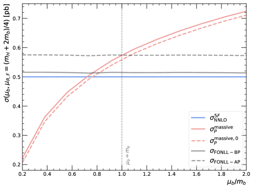
Figure 2: Cancellation of the dependence on the matching scale in the FONLL-AP and FONLL-BP schemes.

First, as a consistency check, in Fig. 2 we verify that indeed the dependence on $\mu_{b}$ cancels when constructing the FONLL result with parametrized $b$ according to Eq. (2.2). In this figure the massive-scheme result has been constructed using a fixed $b$ PDF (that which corresponds to the standard matching condition at $\mu_{b}=m_{b}$) and then re-expressing results in terms of the massive scheme PDFs and $\alpha_{s}$ in terms of massless-scheme ones. This is done using Eq. (8), which contains the matching coefficients $K_{ij}$ which depend on the matching scale $\mu_{b}$, and thus the massive-scheme result becomes $\mu_{b}$-dependent. However, this dependence cancels exactly in the final FONLL result.

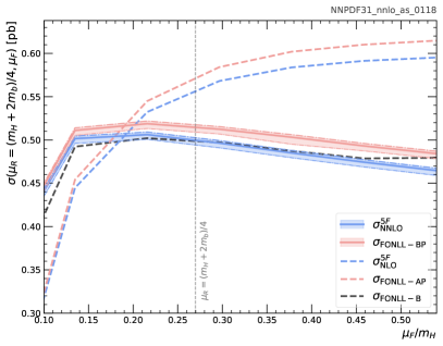
Figure 3: Renormalization (left) and factorization (right) scale variation of the cross-section for Higgs production in bottom fusion. The pure five-flavor scheme computation is compared to the FONLL-AP and FONLL-BP results presented here and to the FONLL-B result of Ref. [13]. For the pure five flavor NNLO and the FONLL-BP three curves are shown, corresponding to three choices of initial $b$ PDF (see text).

In Fig. 3 we show the factorization and renormalization scale dependence of the cross-section computed in various schemes, with the other scale kept fixed at the preferred [13, 14] value $\mu=\frac{m_{H}+2m_{b}}{4}$. Specifically, we compare results obtained using the FONLL-AP and FONLL-BP schemes discussed above, the pure five-flavor scheme , and the FONLL-B result of Ref. [14], all using the same PDFs (including the $b$ PDF) as discussed above. For the pure five-flavor scheme and for FONLL-BP we also show the three curves corresponding to the three different choices for the $b$ PDF discussed above, with a corresponding band: the central, thick, solid line represents the default $\mu_{b}=m_{b}$ choice, while the edges of the band are drawn with dot-dash curves with decreasing thickness, with the thicker of the two corresponding to $\mu_{b}=2\frac{m_{b}}{3}$, and the other two $\mu_{b}=\frac{m_{b}}{2}$.

Note that the FONLL-BP computation Eq. (16) and the FONLL-B result [14] are directly comparable: indeed, they both include the five-flavor scheme computation up to NNLO, and combine it with the first two orders of the massive-scheme computation. The difference is that in FONLL-B in the massive-scheme computation refers to the process $gg\to b\bar{b}H$, while in FONLL-BP it refers to $b\bar{b}\to H$. If the $b$ PDF is the same as given by perturbative matching, the difference is then only that, in the latter case, only mass effects related to the $b\bar{b}$ which fuses into the Higgs are included, while in the former, also those related to the further unobserved $b\bar{b}$ pair are present. In a realistic situation, in which FONLL-BP is used while parametrizing and fitting the $b$ PDF these mass effects should be reabsorbed in the fitted $b$ PDF. In our comparisons, they appear as a certain enhancement of FONLL-BP in comparison to FONLL-B due to the opening of phase space.

Otherwise, the qualitative features of the comparison between FONLL and the pure five-flavor scheme remain essentially the same as discussed in Ref. [14]: FONLL is quite close to the five-flavor scheme, with mass effects a non-negligible, but small, positive correction. Indeed, the difference between FONLL-AP and FONLL-BP, i.e., the impact of NNLO corrections in the five-flavor scheme, is much more significant than that of mass corrections. The impact of varying the $b$ PDF by an amount which is comparable to a reasonable variation of the matching scale is clearly comparable to that of the mass corrections. This provides evidence for the fact that fitting the $b$ PDF is likely to have a significant impact on precision phenomenology.

Note that results for the FONLL-B scheme differ at the percent level from those of Ref. [14] because there a different PDF set and $m_{b}$ value were used, for the sake of benchmarking with Ref. [15, 16]. This further highlights the fact that the size of effects due to the $b$ PDF is comparable to that of mass corrections.

4 Conclusions

In summary, we have shown how the FONLL matching of massive- and massless-scheme treatment of computations involving heavy quarks can be generalized to the case in which the heavy quark PDF is freely parametrized for hadronic processes. We have show that this effectively provides us with a massive heavy quark scheme, in which the heavy quark is endowed with a standard PDF satisfying QCD evolution equations, yet it is treated as massive in hard matrix elements. A first application to Higgs production in bottom fusion shows that effects related to the $b$ PDF are quite likely to be comparable to mass corrections: both are small, but non-negligible corrections to a purely massless NNLO calculation in which the $b$ PDF is obtained from perturbative matching conditions. Determining the $b$ PDF from data is thus likely to be necessary for a description of $b$-induced hadron collider processes at percent or sub-percent accuracy.

As a direction for further study, it should be noticed that extending our results to NNLO — thereby allowing the construction of a FONLL-CP result, in the terminology of Sect. 2.1 (NNLO+NNLL) — is beyond current knowledge. Indeed, starting at NNLO the cancellation between real and virtual corrections is no longer trivial, and is spoiled by massive quarks in the initial state [26, 27]. Hence, such an extension would require conceptual advances in the understanding of QCD factorization in the presence of massive quarks, which are left for future studies.

Appendix A Matching coefficients

We collect for ease of reference the well-known matching coefficients which relate the four and five scheme PDFs. Up to $O(\alpha_{s})$

$$K_{ij}(z,Q^{2})=\delta_{ij}\delta(1-z)+\alpha_{s}(Q^{2})\,K_{ij}^{(1)}(z,Q^{2})+{\cal O}(\alpha_{s}^{2})\,.$$ (A.1)

so that

$$K_{ij}^{-1}(z,Q^{2})=\delta_{ij}\delta(1-z)-\alpha_{s}(Q^{2})\,K_{ij}^{(1)}(z,Q^{2})+{\cal O}(\alpha_{s}^{2})\,.$$ (A.2)

The only non-zero contributions at order ${\cal O}(\alpha_{s})$ are the heavy quark-heavy quark and the heavy quark-gluon matching functions, which are respectively given by

$$\begin{split}K_{bb}^{(1)}\left(x,\frac{Q^{2}}{\mu_{b}^{2}}\right)&=\frac{C_{F}}{2\,\pi}{\left\{P_{qq}(x)\left[\ln{\frac{Q^{2}}{\mu_{b}^{2}}}-2\ln(1-x)-1\right]\right\}}_{+}\\ K_{bg}^{(1)}\left(x,\frac{Q^{2}}{\mu_{b}^{2}}\right)&=\frac{T_{R}}{2\,\pi}P_{qg}(x)\,\ln{\frac{Q^{2}}{\mu_{b}^{2}}}\end{split}$$ (A.3)

where

$$P_{qg}(x)=\left(1\,-\,2\,x\,+\,2\,x^{2}\right)\quad{\rm and}\quad P_{qq}(x)=\frac{2}{1-x}-\left(1+x\right)\,.$$ (A.4)

Appendix B Massive coefficient functions

In this Appendix we summarize the computation of the coefficient functions in the massive scheme and of their massless limit up to $O(\alpha_{s})$. The NLO corrections are computed using the extension of Catani-Seymour subtraction for massive initial states developed in Ref. [19] and extended to QCD in Ref. [7]. This way of preforming the computation has the main advantage of following closely that of the five-flavor massive scheme, so that a direct comparison is much easier at the analytic level. Indeed, strictly speaking because of Eq. (15) the massless limit is not needed. However, we have computed it explicitly in order to check that it matches the massless-scheme result (thereby verifying Eq. (14) explicitly), and also in order to produce Fig. 2, which provides a further consistency check. Another advantage of this way of performing the computation (though we do not use it here) is that it allows for the computation of the fully differential cross section in this scheme.

B.1 Leading order

The leading order partonic cross section for the production of a Higgs boson, accounting for the mass of the initial state $b$ and $\bar{b}$, is given by

$$\hat{\sigma}_{0}(xs)=\left(\frac{g_{b\bar{b}H}^{2}\,\beta_{0}\,\pi}{6}\right)\delta(xs-m_{H}^{2})=\sigma_{0}\,x\,\delta\left(x-\frac{m_{H}^{2}}{s}\right)$$ (B.1)

where

$$\sigma_{0}=\frac{g_{b\bar{b}H}^{2}\,\beta_{0}\,\pi}{6\,m_{H}^{2}}\,,\quad{\rm and}\quad\beta_{0}=\sqrt{1-\frac{4\,m_{b}^{2}}{m_{H}^{2}}}\,.$$ (B.2)

where $g_{b\bar{b}H}$ is the coupling of the $b$ quark to the Higgs boson, obtained as the mass of the quark divided by vacuum expectation value of the Higgs sector:

$$g_{b\bar{b}H}=\frac{m_{b}}{v}\,.$$ (B.3)

In the following we will also use the notation

$${\cal B}(x)\equiv\hat{\sigma}_{0}(xs)\,,\quad{\rm and}\quad{\cal B}\equiv\hat{\sigma}_{0}(s)\,.$$ (B.4)

B.2 Next-to-leading order: $b\bar{b}$-channel

The next to leading order corrections to the Higgs production in bottom quark fusion consist in virtual corrections (${\cal V}$) to the left diagram of Fig. 1, as well as of real emission corrections (${\cal R}$) , represented by the central diagram of Fig. 1. Both this contributions are separately divergent when the additional gluon, real or virtual, becomes soft, though the final result remains finite. In order to handle these soft divergences we employ the subtraction scheme defined in [7]. This implies that we need two more ingredients: a subtraction term, ${\cal S}$, and its integral over the gluon phase space, ${\cal I}=\int{\rm d}\Phi_{g}{\cal S}$. Our final result is then given by:

$$\hat{\sigma}_{\rm NLO}=\int{\rm d}\Phi_{1}{\cal B}+{\cal V}+{\cal I}+\int{\rm d}\Phi_{2}{\cal R}-{\cal S}\,.$$ (B.5)

B.2.1 Real corrections, and subtraction term

The real emission partonic differential cross section, is given by

$$\int{\rm d}\Phi_{2}{\cal R}=\int{\rm d}\Phi_{2}\left|\overline{{\cal M}}_{b\bar{b}Hg}\right|(s,t,u)\,,$$ (B.6)

where

$${\rm d}\Phi_{2}=\frac{1}{32\,\pi\,\beta\,s}{\rm d}\cos\theta\,\Theta(1+\cos\theta)\,\Theta(1-\cos\theta)\,,\quad{\rm and}\quad\beta=\sqrt{1-\frac{4\,m_{b}^{2}}{s}}\,,$$ (B.7)

and

$$\begin{split}\left|\overline{{\cal M}}_{b\bar{b}Hg}\right|(s,t,u)=&\frac{4}{3}\pi g_{b\bar{b}H}^{2}C_{F}\alpha_{s}\left\{\left(s-m_{H}^{2}\right)\left[\frac{1}{m_{b}^{2}-t}+\frac{1}{m_{b}^{2}-u}\right]\right.\\ &\left.+(m_{H}^{2}-4\,m_{b}^{2})\left[\frac{2\left(s-2\,m_{b}^{2}\right)}{(m_{b}^{2}-t)(m_{b}^{2}-u)}-\frac{2\,m_{b}^{2}}{(m_{b}^{2}-t)^{2}}-\frac{2\,m_{b}^{2}}{(m_{b}^{2}-u)^{2}}\right]\right\}\,.\end{split}$$ (B.8)

The Mandelstam variables in terms of scalar products and $\cos\theta$ are given by

$$\left\{\begin{split}t&=m_{b}^{2}-\frac{s-m_{H}^{2}}{2}\left(1-\beta\,\cos\theta\right)\\ u&=m_{b}^{2}-\frac{s-m_{H}^{2}}{2}\left(1+\beta\,\cos\theta\right)\end{split}\right.\,.$$ (B.9)

In order to remove the soft divergence which appears in the $s\rightarrow m_{H}^{2}$ limit we need to construct a suitable subtraction term. Using the relevant equations in Ref. [7] we find

$${\cal S}=\frac{2}{3}\,\pi\,\alpha_{s}\,C_{F}\,g_{b\bar{b}H}^{2}\,\beta_{0}^{2}\,m_{H}^{2}\frac{1}{\tilde{x}}\left[\frac{2}{m_{b}^{2}-t}\left(P_{qq}(\tilde{x})-\frac{2\,\tilde{x}\,m_{b}^{2}}{m_{b}^{2}-t}\right)+\frac{2}{m_{b}^{2}-u}\left(P_{qq}(\tilde{x})-\frac{2\,\tilde{x}\,m_{b}^{2}}{m_{b}^{2}-u}\right)\right]$$ (B.10)

where

$$\tilde{x}=\frac{m_{H}^{2}-2\,m_{b}^{2}}{s-2\,m_{b}^{2}}\,.$$ (B.11)

Combining Eqs. (B.8) and (B.10) and factoring the trivial $\frac{\alpha_{s}\,C_{F}\,\sigma_{0}}{\pi}$ dependence we get

$$\begin{split}\frac{\alpha_{s}\,C_{F}\,\sigma_{0}}{\pi}\int{\rm d}\Phi_{2}\left[{\cal R}-{\cal S}\right]&=\frac{\alpha_{s}\,C_{F}\,\sigma_{0}}{\pi}\frac{m_{b}^{2}}{2}\int_{-1}^{1}{\rm d}\cos\theta\left[\frac{s\,(s-m_{H}^{2})^{2}}{(m_{H}^{2}-2\,m_{b}^{2})(m_{b}^{2}-t)(m_{b}^{2}-u)}\right]\\ &=-\frac{\alpha_{s}\,C_{F}\,\sigma_{0}}{\pi}\frac{1}{\beta_{0}}\left(\frac{1-\beta^{2}}{\beta^{2}}\right)\frac{x}{\left(1-2\,x-\beta^{2}\right)}\ln d\,,\end{split}$$ (B.12)

where we defined

$$d\equiv\frac{1+\beta}{1-\beta}\,,\quad{\rm and}\quad x\equiv\frac{m_{H}^{2}}{s}\,.$$ (B.13)

B.2.2 Virtual corrections, and integrated subtraction term

QCD virtual corrections to the Born process in this simple case completely factorize in a vertex form factor:

$${\cal V}=\frac{\alpha_{s}\,C_{F}}{\pi}{\cal B}\,\delta_{g}\,,$$ (B.14)

with

$$\delta_{g}=-1-L_{\lambda}+\frac{(1-\beta_{0}^{2})}{\beta_{0}}\ln d_{0}-\frac{1+\beta_{0}^{2}}{2\,\beta_{0}}\left[-\ln d_{0}\,L_{\lambda}+\ln^{2}d_{0}+{\rm Li}_{2}\left(1-\frac{1}{d_{0}}\right)-\frac{\pi^{2}}{2}\right]\,,$$ (B.15)

where

$$L_{\lambda}\equiv\frac{1}{\epsilon}+\ln\frac{4\,\pi\,\mu_{R}^{2}}{m_{b}^{2}}+{\cal O}(\epsilon^{2})\,.$$ (B.16)

The integrated subtraction term ${\cal I}$ is obtained by integrating ${\cal S}$, Eq. (B.10), over the phase space of the emitted gluon. This term can be separated into two pieces: a term proportional to $\delta(1-x)$, which contains the singularity, and a plus distribution:

$${\cal I}=\delta(1-x)\,I+\left\{{\cal G}(x)\right\}_{+}\,,$$ (B.17)

where

$$\begin{split}I=&2+L_{\lambda}-\ln{\frac{(1+\beta_{0}^{2})^{2}}{1-\beta_{0}^{2}}}+\frac{1-3\,\beta_{0}^{2}}{4\beta_{0}}\ln d_{0}\\ &+\frac{1+\beta_{0}^{2}}{2\,\beta_{0}}\left[\frac{1}{2}\ln^{2}d_{0}-\ln d_{0}\,\ln{\frac{4\,\beta_{0}^{2}}{(1+\beta)^{2}}}-L_{\lambda}\,\ln d_{0}-1+2\,{\rm Li}_{2}\left(\frac{1}{d_{0}}\right)-\frac{\pi^{2}}{3}\right]\,,\end{split}$$ (B.18)

and

$$\{{\cal G}(x)\}_{+}={\left\{P_{qq}(x)\left[\frac{1+\beta^{2}}{2\beta}\ln{d}-1\right]+\left(1-x\right)\right\}}_{+}\,.$$ (B.19)

B.2.3 Final formulae, mass and PDF renormalization

We now combine the various partial results obtained in the previous subsections into the full expression for the $b\bar{b}$-channel coefficient functions. First, however, we need to adjust $b$-quark mass and the PDFs. Renormalization of the $b$ mass leads to the replacement

$$g_{hb\bar{b}}^{2}=g_{hb\bar{b}}^{2}(\mu_{R}^{2})\left(1-\frac{\alpha_{s}\,C_{F}}{\pi}\left(\frac{3}{2}\ln\frac{m_{b}^{2}}{\mu_{R}^{2}}-2\right)\right)\,.$$ (B.20)

in $\sigma_{0}$, Eq. (B.2).

The massive $b$ PDF is free of collinear singularities and thus it does not have to undergo subtraction: indeed it is scale independent. However, we must perform the change of renormalization scheme Eq. (11) which relates the massive and massless schemes. Up to ${\cal O}(\alpha_{s})$ we get

$$B_{b\bar{b}}\left(x,\mu_{R}^{2},\mu_{F}^{2},\mu_{b}^{2}\right)=\,\left[\sigma_{0}(\mu_{R}^{2})\delta(1-x)+\alpha_{s}(\mu_{R}^{2})B_{b\bar{b}}^{(1)}\left(x,\mu_{R}^{2},\mu_{F}^{2},\mu_{b}^{2}\right)\right]+{\cal O}(\alpha_{s}^{2})$$ (B.21)

where

$$\begin{split}B_{b\bar{b}}^{(1)}\left(x,\mu_{R}^{2},\mu_{F}^{2},\mu_{b}^{2}\right)=\frac{\sigma_{0}(\mu_{R}^{2})\,C_{F}}{\pi}&\left\{\left[\frac{3}{2}\ln\frac{\mu_{R}^{2}}{\mu_{b}^{2}}+2+I+\delta_{g}\right]\delta(1-x)\right.\\ &\left.+\int_{0}^{1}{\rm d}z\{{\cal G}(z)-2\,K_{b\bar{b}}^{(1)}(z)\}_{+}z\,\delta(z-x)+\int{\rm d}\Phi_{2}\left[{\cal R}-{\cal S}\right]\right\}\,.\end{split}$$ (B.22)

Performing the $z$ integration gives the final result

$$\begin{split}B_{b\bar{b}}^{(1)}&\left(x,\mu_{R}^{2},\mu_{F}^{2},\mu_{b}^{2}\right)=\frac{\sigma_{0}(\mu_{R}^{2})\,C_{F}}{\pi}\Biggl{\{}\delta(1-x)\left[\xi-2+\frac{3}{2}\left(\gamma_{0}\ln\frac{(1+\beta)^{2}}{4}-\gamma_{0}\ln\frac{m_{H}^{2}}{m_{b}^{2}}+\ln\frac{\mu_{R}^{2}}{\mu_{F}^{2}}\right)\right]\\ +&\,4\,{\cal D}_{1}(1-x)+2\left[\gamma\ln\frac{(1+\beta)^{2}}{4}+\gamma\ln\frac{m_{H}^{2}}{m_{b}^{2}}+\ln{\frac{\mu_{b}^{2}}{\mu_{F}^{2}}}\right]\,{\cal D}_{0}(1-x)\\ -&(2+x+x^{2})\left[\gamma\ln\frac{(1+\beta)^{2}}{4}+\gamma\ln\frac{m_{H}^{2}}{m_{b}^{2}}-\gamma\ln x+\ln{\frac{\mu_{b}^{2}}{\mu_{F}^{2}}}+2\ln(1-x)\right]+x\,(1-x)\\ -&\frac{2\,\gamma\,\ln x}{1-x}-\frac{1}{\beta_{0}}\left(\frac{1-\beta^{2}}{\beta^{2}}\right)\frac{x}{\left(1-2\,x-\beta^{2}\right)}\ln d\Biggr{\}}\,,\end{split}$$ (B.23)

where

$$\xi=1+\ln\left(\frac{1-\beta_{0}^{2}}{(1+\beta_{0})^{2}}\right)+\frac{\left(5-7\beta_{0}^{2}\right)}{4\,\beta_{0}}\ln d_{0}+\frac{\left(\beta_{0}^{2}+1\right)}{\beta_{0}}\left(2\,{\rm Li}_{2}\left(\frac{1}{d_{0}}\right)+\frac{\pi^{2}}{6}-\ln d_{0}\ln\frac{4\beta_{0}^{2}}{(1+\beta_{0}^{2})(1+\beta_{0})}\right)\,,$$ (B.24)

and

$$\gamma=\frac{1+\beta^{2}}{2\,\beta}\,,\quad\gamma_{0}=\frac{1+\beta_{0}^{2}}{\,2\beta_{0}}\,\quad\text{ and }\quad{\cal D}_{n}(x)={\left(\frac{\ln^{n}(1-x)}{1-x}\right)}_{+}\,.$$ (B.25)

B.2.4 Massless limit

The massless limit of the $b\bar{b}$-channel can be computed directly from Eq. (B.23), by setting $\beta=1$ everywhere except in the logarithms, where one can use the simple expansion

$$\beta\sim 1\,-\,\frac{2\,x\,m_{b}^{2}}{m_{H}^{2}}+{\cal O}\left(\frac{m_{b}^{4}}{m_{H}^{4}}\right)\,.$$ (B.26)

We get

$$\begin{split}B_{b\bar{b}}^{(1),(0)}&\left(x,\mu_{R}^{2},\mu_{F}^{2},\mu_{b}^{2}\right)=\frac{\alpha_{s}\,C_{F}\,\sigma_{0}(\mu_{R}^{2})}{\pi}\Biggl{\{}\delta(1-x)\left[-1+\frac{\pi^{2}}{3}+\frac{3}{2}\ln\frac{\mu_{R}^{2}}{\mu_{F}^{2}}\right]+\,4\,{\cal D}_{1}(1-x)\\ +&2\left(\ln{\frac{m_{H}^{2}}{\mu_{F}^{2}}}+\ln{\frac{\mu_{b}^{2}}{m_{b}^{2}}}\right)\,{\cal D}_{0}(1-x)-\frac{2\ln x}{1-x}-(2+x+x^{2})\left[\ln\frac{m_{H}^{2}}{\mu_{F}^{2}}+\ln{\frac{\mu_{b}^{2}}{m_{b}^{2}}}+\ln\frac{(1-x)^{2}}{x}\right]+x\,(1-x)\Biggr{\}}\,.\end{split}$$ (B.27)

As it can be easily verified, this exactly corresponds to its massless scheme equivalent, which can be found in Eq. (A6) of Ref. [28].

B.3 Next-to-leading order: $bg$-channel

In the presence of initial-state massive quarks, the cross-section for the $bg$-channel is free of soft or collinear divergences, and no subtraction is accordingly necessary. Also in this case, however, we must perform the scheme change Eq. (11). We get

$$\begin{split}B_{bg}^{(1)}(x,\mu_{R}^{2},\mu_{F}^{2},\mu_{b}^{2})&=\hat{\sigma}_{bg}(x,\mu_{R}^{2})-\alpha_{s}\,\int_{0}^{1}{\rm d}z\,K_{bg}^{(1)}(z,\mu_{F}^{2})\sigma(zs)\,\\ &=\left.\hat{\sigma}_{bg}(x,\mu_{R}^{2})-\frac{\alpha_{s}\,T_{R}\,\sigma_{0}}{\pi}\left[\frac{x}{2}\,P_{qg}(x)\ln{\frac{\mu_{F}^{2}}{\mu_{b}^{2}}}\right]\,\right|_{x=\tfrac{m_{H}^{2}}{s}},\end{split}$$ (B.28)

where

$$\hat{\sigma}_{bg}(x,\mu_{R}^{2})=\int{\rm d}\Phi_{2}^{(b)}\left|\overline{{\cal M}}_{bgHb}\right|^{2}(s,t,u)\,,$$ (B.29)

and the subscript $(b)$ in $\Phi_{2}^{(b)}$ denotes the fact that now the phase-space has a massive $b$ instead of a massless gluon, in the final state. The color- and helicity-averaged square matrix element, can be obtained from Eq. (B.8) using crossing symmetry. In addition, we have to take into account that the gluon can have 8 possible colors (as opposed to 3 for a quark),

$$\left|\overline{{\cal M}}_{bgHb}\right|^{2}(s,t,u)=-\frac{3}{8}\left|\overline{{\cal M}}_{b\bar{b}Hg}\right|^{2}(t,s,u)\,,$$ (B.30)

where now the Mandelstam invariants are given by

$$\left\{\begin{split}t&=2\,m_{b}^{2}+\frac{s}{32}\left((5-\beta^{2})(\beta^{2}+4\,x-5)-(3+\beta^{2})\,\Lambda\,\cos\theta\right)\\ u&=m_{b}^{2}+\frac{s}{32}\left((5-\beta^{2})(\beta^{2}+4\,x-5)+(3+\beta^{2})\,\Lambda\,\cos\theta\right),\end{split}\right.\,$$ (B.31)

where

$$\Lambda=\sqrt{\left(3+\beta^{2}\right)^{2}+16x^{2}-8\,x\,\left(5-\beta^{2}\right)}\,,$$ (B.32)

while the phase-space ${\rm d}\Phi_{2}^{(b)}$ is given by

$${\rm d}\Phi_{2}^{(b)}=\frac{\Lambda\,x}{32\,\pi\,\left(3+\beta^{2}\right)\,m_{H}^{2}}\,{\rm d}\cos\theta\,\Theta(1+\cos\theta)\,\Theta(1-\cos\theta)\,.$$ (B.33)

Performing the $\cos\theta$ integration gives

$$\begin{split}\hat{\sigma}_{bg}(x,\mu_{R}^{2})=&\frac{\alpha_{s}\,T_{R}\,\sigma_{0}(\mu_{R}^{2})}{\pi}\frac{x}{16\beta_{0}\left(\beta^{2}+3\right)^{3}}\\ &\times\Biggl{\{}-64\left(9\beta^{4}+(40x-42)\beta^{2}+8x(4x-9)+49\right){\rm arctanh}\left(\frac{\Lambda}{\beta^{2}+4x-5}\right)\\ &\frac{4096\,\Lambda\,\left(1-\beta^{2}\right)\left(\beta^{2}+x-1\right)}{\left(-\Lambda+\beta^{2}+4x-5\right)\left(\Lambda+\beta^{2}+4x-5\right)}+\Lambda\,\left(5-\beta^{2}\right)\left(\beta^{4}+(4x+22)\beta^{2}+44x-71\right)\Biggr{\}}\,.\end{split}$$ (B.34)

B.3.1 Massless limit

As in the case of the $b\bar{b}$ channel, taking the massless limit requires setting $\beta=1$ everywhere except in the logarithms where one can use Eq. (B.26), which gives

$$B_{bg}^{(1),(0)}(x,\mu_{R}^{2},\mu_{F}^{2},\mu_{b}^{2})=\frac{T_{R}}{\pi}\left\{\frac{x}{2}\,P_{qg}(x)\left[\ln\left(\frac{(1-x)^{2}}{x}\right)+\ln\frac{m_{H}^{2}}{\mu_{F}^{2}}+\ln{\frac{\mu_{b}^{2}}{m_{b}^{2}}}\right]-\frac{x}{4}(1-x)(3-7\,x)\right\}\,.$$ (B.35)

Once again, one can explicitly check that this exactly corresponds to its massless scheme counterpart, which can be found in Eq. (A9) of Ref. [28].

References

- [1] R. D. Ball et al., Parton distributions from high-precision collider data, Eur. Phys. J. C77 (2017), no. 10 663, [arXiv:1706.00428].
- [2] S. J. Brodsky, P. Hoyer, C. Peterson, and N. Sakai, The Intrinsic Charm of the Proton, Phys. Lett. 93B (1980) 451–455.
- [3] S. J. Brodsky, C. Peterson, and N. Sakai, Intrinsic Heavy Quark States, Phys. Rev. D23 (1981) 2745.
- [4] F. Maltoni, G. Ridolfi, and M. Ubiali, b-initiated processes at the LHC: a reappraisal, JHEP 07 (2012) 22, [arXiv:1203.6393].
- [5] M. Lim, F. Maltoni, G. Ridolfi, and M. Ubiali, Anatomy of double heavy-quark initiated processes, JHEP 09 (2016) 132, [arXiv:1605.09411].
- [6] E. Bagnaschi, F. Maltoni, A. Vicini, and M. Zaro, Lepton-pair production in association with a pair and the determination of the boson mass, arXiv:1803.04336.
- [7] F. Krauss and D. Napoletano, Towards a fully massive five-flavor scheme, Phys. Rev. D98 (2018), no. 9 096002, [arXiv:1712.06832].
- [8] D. Figueroa, S. Honeywell, S. Quackenbush, L. Reina, C. Reuschle, and D. Wackeroth, Electroweak and QCD corrections to -boson production with one jet in a massive five-flavor scheme, Phys. Rev. D98 (2018), no. 9 093002, [arXiv:1805.01353].
- [9] R. D. Ball, V. Bertone, M. Bonvini, S. Forte, P. Groth Merrild, J. Rojo, and L. Rottoli, Intrinsic charm in a matched general-mass scheme, Phys. Lett. B754 (2016) 49–58, [arXiv:1510.00009].
- [10] R. D. Ball, M. Bonvini, and L. Rottoli, Charm in Deep-Inelastic Scattering, JHEP 11 (2015) 122, [arXiv:1510.02491].
- [11] R. D. Ball, V. Bertone, M. Bonvini, S. Carrazza, S. Forte, A. Guffanti, N. P. Hartland, J. Rojo, and L. Rottoli, A Determination of the Charm Content of the Proton, Eur. Phys. J. C76 (2016), no. 11 647, [arXiv:1605.06515].
- [12] M. Cacciari, M. Greco, and P. Nason, The P(T) spectrum in heavy flavor hadroproduction, JHEP 9805 (1998) 7, [hep-ph/9803400].
- [13] S. Forte, D. Napoletano, and M. Ubiali, Higgs production in bottom-quark fusion in a matched scheme, Phys. Lett. B751 (2015) 331–337, [arXiv:1508.01529].
- [14] S. Forte, D. Napoletano, and M. Ubiali, Higgs production in bottom-quark fusion: matching beyond leading order, Phys. Lett. B763 (2016) 190–196, [arXiv:1607.00389].
- [15] M. Bonvini, A. S. Papanastasiou, and F. J. Tackmann, Resummation and matching of b-quark mass effects in production, JHEP 11 (2015) 196, [arXiv:1508.03288].
- [16] M. Bonvini, A. S. Papanastasiou, and F. J. Tackmann, Matched predictions for the cross section at the 13 TeV LHC, JHEP 10 (2016) 53, [arXiv:1605.01733].
- [17] D. de Florian et al., Handbook of LHC Higgs Cross Sections: 4. Deciphering the Nature of the Higgs Sector, arXiv:1610.07922.
- [18] S. Forte, E. Laenen, P. Nason, and J. Rojo, Heavy quarks in deep-inelastic scattering, Nucl.Phys. B834 (2010) 116–162, [arXiv:1001.2312].
- [19] S. Dittmaier, A general approach to photon radiation off fermions, Nucl. Phys. B565 (2000) 69–122, [9904440].
- [20] M. Buza, Y. Matiounine, J. Smith, and W. L. van Neerven, Charm electroproduction viewed in the variable flavor number scheme versus fixed order perturbation theory, Eur. Phys. J. C1 (1998) 301–320, [hep-ph/9612398].
- [21] R. V. Harlander and W. B. Kilgore, Next–to-next–to–leading order Higgs production at hadron colliders, Phys.Rev.Lett. 88 (2002) 201801, [hep-ph/0201206].
- [22] S. Forte, D. Napoletano, and M. Ubiali, “bbhfonll.” http://bbhfonll.hepforge.org/, 2017.
- [23] J. Alwall, R. Frederix, S. Frixione, V. Hirschi, F. Maltoni, O. Mattelaer, H.-S. Shao, T. Stelzer, P. Torrielli, and M. Zaro, The automated computation of tree-level and next-to-leading order differential cross sections, and their matching to parton shower simulations, JHEP 1407 (2014) 79, [arXiv:1405.0301].
- [24] M. Wiesemann, R. Frederix, S. Frixione, V. Hirschi, F. Maltoni, and P. Torrielli, Higgs production in association with bottom quarks, JHEP 02 (2015) 132, [arXiv:1409.5301].
- [25] A. Buckley, J. Ferrando, S. Lloyd, K. Nordström, B. Page, M. Rüfenacht, M. Schönherr, and G. Watt, LHAPDF6: parton density access in the LHC precision era, Eur. Phys. J. C75 (2015), no. 3 132, [arXiv:1412.7420].
- [26] R. Doria, J. Frenkel, and J. C. Taylor, Counter Example to Nonabelian Bloch-Nordsieck Theorem, Nucl. Phys. B168 (1980) 93–110.
- [27] S. Catani, M. Ciafaloni, and G. Marchesini, Non-cancelling infrared divergences in QCD coherent state, Nucl. Phys. B264 (1986) 588–620.
- [28] R. V. Harlander and W. B. Kilgore, Higgs boson production in bottom quark fusion at next-to-next-to leading order, Phys. Rev. D68 (2003) 13001, [hep-ph/0304035].