Investigating the Diversity of Type Ia Supernova Spectra with the Open-Source Relational Database Kaepora

Abstract

We present a public, open-source relational database (we name kaepora) containing a sample of 4975 spectra of 777 Type Ia supernovae (SNe Ia). Since we draw from many sources, we significantly improve the spectra by inspecting these data for quality, removing galactic emission lines and cosmic rays, generating variance spectra, and correcting for the reddening caused by both MW and host-galaxy dust. With our database, we organize this homogenized dataset by 56 unique categories of SN-specific and spectrum-specific metadata. With kaepora, we produce composite spectra of subpopulations of SNe Ia and examine how spectral features correlate with various SN properties. These composite spectra reproduce known correlations with phase, light-curve shape, and host-galaxy morphology. With our large dataset, we are also able to generate fine-grained composite spectra simultaneously over both phase and light-curve shape. The color evolution of our composite spectra is consistent with other SN Ia template spectra, and the spectral properties of our composite spectra are in rough agreement with these template spectra with some subtle differences. We investigate the spectral differences of SNe Ia that occur in galaxies with varying morphologies. Controlling for light-curve shape, which is highly correlated with host-galaxy morphology, we find that SNe Ia residing in late-type and early-type galaxies have similar spectral properties at multiple epochs. However for SNe Ia in these different environments, their spectra appear to have Ca II near-infrared triplet features that have slightly different strengths. Although this is apparent in the composite spectra and there is some difference in the populations as seen by individual spectra, this difference is not large enough to indicate differences in the underlying populations. All individual spectra and metadata are available in our open-source database kaepora along with the tools developed for this investigation to facilitate future investigations of SN Ia properties.

1 Introduction

Type Ia (SNe Ia) are excellent cosmological probes and an important tool for understanding dark energy. In general, the accepted models for these phenomena involve the thermonuclear disruption of a carbon-oxygen white dwarf. Despite their reputation as “standard candles", the observational properties of these explosions are intrinsically heterogeneous (Hatano et al., 2000; Blondin et al., 2012a). SN Ia luminosities can vary by an order of magnitude (Pskovskii, 1977). The “standardizability” of these events only became evident after observing some basic correlations between these optical properties. Mainly, SNe Ia exhibit an empirical relationship between peak luminosity and light-curve width (Pskovskii, 1977; Phillips, 1993; Riess et al., 1996). This relationship has been attributed to the varying amount of ⁵⁶Ni produced in these explosions (Arnett, 1982; Nugent et al., 1995; Stritzinger et al., 2006).

The normalization of SN Ia luminosities via this relationship allows for precise distance measurements on extragalactic scales. Measurements of SNe Ia were used to show that the expansion of our universe is currently accelerating (Riess et al., 1998; Perlmutter et al., 1999). Today, after making corrections for light-curve shape and color, there remains an intrinsic scatter that may belie unaccounted SN physics (Foley & Kasen, 2011; Scolnic et al., 2018; Jones et al., 2018). This scatter will soon become a dominant source of systemic uncertainty for SN Ia distance measurements (Jones et al., 2018).

Although valuable, these basic correlations do not adequately explain the observed spectral diversity. For example, SNe Ia with the same light-curve shape and color exhibit a wide range of photospheric velocities at maximum light (Hatano et al., 2000). Spectra provide an abundance of information about SN ejecta (e.g., nucleosynthesis, ionization states, kinematics, etc.) necessary for constructing a complete picture of these phenomena.

Despite their proven cosmological utility, open questions remain regarding the physical processes that can produce the observed range of diversity. Detailed studies of individual events have been essential for improving our understanding of how spectral features change with phase and luminosity. The well-sampled spectroscopic observations of SN 2011fe solidified our understanding of the optical properties of normal SNe Ia from very early to very late epochs (Nugent et al., 2011; Pereira et al., 2013a; Shappee et al., 2013; Mazzali et al., 2014a). Observations of the spectroscopically distinct SNe 1991T (Phillips et al., 1992; Filippenko et al., 1992c) and 1991bg (Filippenko et al., 1992a; Leibundgut et al., 1993) highlight how the temperature of the SN ejecta can impact spectral features. SN 1991T exhibited a large intrinsic luminosity and showed very little Ca H&K and Si II $\lambda 5972$ absorption. In addition to its low intrinsic luminosity, SN 1991bg showed strong Ti II absorption near $4300$ Å at maximum light. These effects have been attributed to a sequence in the photospheric temperature where peculiar events like SNe 1991T and 1991bg lie in the high- and low-temperature tails of this relationship, respectively (Nugent et al., 1995). This sequence could be described by the tight correlation between light-curve shape and the ratio of the depth Si II $\lambda 5972$ and $\lambda 6355$ ($\mathcal{R}$(Si II)). While very useful, detailed analyses of a few individual events cannot fully represent the observed spectroscopic diversity.

Branch (1987) first showed that ejecta velocities of SNe Ia are heterogeneous. Studies of larger samples have revealed that the nature of the diversity of SNe Ia properties is indeed multidimensional (Hatano et al., 2000; Li et al., 2001b; Benetti et al., 2005; Foley et al., 2011; Blondin et al., 2012a). For normal SNe Ia, the velocities derived from Si II $\lambda 6355$ do not correlate with the decline-rate parameter $\Delta m_{15}(B)$ (Hatano et al., 2000). Foley & Kasen (2011) showed that high-velocity (HV) SNe Ia have redder intrinsic colors. Furthermore, subgroups of SNe Ia exhibit a large range of velocity gradients for the Si II $\lambda 6355$ feature. Benetti et al. (2005) showed that for normal SNe Ia, this velocity gradient does not correlate with $\Delta m_{15}(B)$. Additional observations have also revealed the presence of high-velocity features (HVF) in numerous events. These typically appear as double-troughed absorption profiles in Si II $\lambda 6355$, Ca II H&K, or the Ca II near-infrared triplet (Gerardy et al., 2004; Mazzali et al., 2005a; Mazzali et al., 2005b; Foley et al., 2012; Childress et al., 2013; Silverman et al., 2015). HVF strength was shown to correlate with the maximum-light velocity of Si II $\lambda 6355$ (Childress et al., 2014). Filling this photometric and spectroscopic parameter space has proven difficult even with large individual SN data sets.

Studies of the mean spectroscopic properties of SNe Ia have been particularly useful for cosmology. Distance estimators require spectral models so that photometric measurements can be calibrated. Spectral models are also useful for estimating bolometric luminosities and thus ⁵⁶Ni yields (Howell et al., 2009). Nugent et al. (2002) first developed a spectral template for the purpose of representing the temporal evolution of normal SNe Ia. Similarly, Hsiao et al. (2007) constructed a mean spectral template time series using ${\sim}600$ spectra of $\sim$100 normal SNe Ia. Sparse sampling of the observed spectroscopic diversity has limited most data-driven spectral templates to single-parameter models (typically phase). The Nugent and Hsiao template spectra are only representative of normal SNe Ia and do not vary with $\Delta m_{15}(B)$. To best represent the heterogeneous nature of SNe Ia, all available spectroscopic data and metadata should be compiled.

Large efforts have been made to improve the accessibility of spectroscopic SN data. Online databases such as SUSPECT (Richardson et al., 2001), WISEREP (Yaron & Gal-Yam, 2012), and the Open Supernova Catalog (Guillochon et al., 2017a) have all provided access to large samples of spectra covering decades of observations. However, since the origins of these data are heterogeneous, studying the bulk properties of these data has been challenging. These spectra have been reduced using different techniques and come from a variety of telescopes and instruments. Thus, the available spectra vary greatly in many basic properties (e.g., wavelength coverage, resolution, signal-to-noise ratio, reduction quality, existence of telluric correction, variance spectra, etc.) Furthermore, online databases do not often link these samples to their respective calibrated light-curves and photometric metadata. While some groups have released large homogenized spectroscopic samples (Blondin et al., 2012a; Silverman et al., 2012a; Folatelli et al., 2013a), no efforts have been made to make use of all available SN Ia spectra at once.

In order to properly combine these data, we have developed a framework to homogenize these spectra. By taking steps like inspecting individual spectra for quality, removing unwanted features, generating variance spectra, correcting for Milky-Way (MW) extinction, and interpolating to constant resolution, we are able to provide a fully homogenized sample containing 4975 spectra of 777 SNe Ia and their associated event specific and spectrum specific metadata. One way we aim to improve the efficiency of SN Ia analyses is via leveraging the power of relational queries. A relational database model simplifies data retrieval and provides a structure that is easily scalable in order to accommodate the rapidly increasing number of SN observations. In this work, we present a comprehensive relational database for observations of SNe Ia. We generate composite spectra from subsets of the data in order to validate the data itself and our processing techniques. The database used in this work and all composite spectra presented below can be found online. The source code developed here is open and freely available for use. Installation instructions and example code are also available online. Here we outline how to query the database for subsamples of individual spectra, and produce composite spectra if desired.

In Section 2, we overview the demographics of the dataset. In Section 3, we outline the reprocessing steps that we execute to homogenize all spectroscopic data and the methods we use for spectroscopic analyses. In Section 4 we present our composite spectra generated from various subsets of these data, compare these composites spectra with other template spectra, and use these composite spectra to investigate SN Ia spectral variations related to their host-galaxy environments. Finally in Section 5, we summarize our results and discuss the future potential for uses of our relational database.

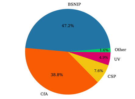
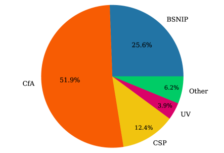
Figure 1: (left): Contributions of each major data source to the total number of SNe in the database. (right): Contributions of each major data source to the total number of spectra in the database. The BSNIP sample provides the largest number of individual SNe, while the CfA sample tends to provide the largest number of spectra per SN.

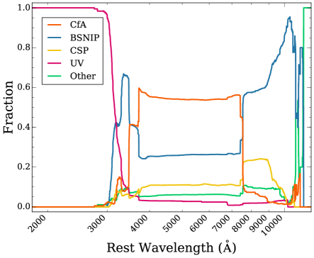
Figure 2: Fraction of all spectra coming from the major sources as a function of wavelength. The CfA sample is the dominant source of spectra in the range of ${\sim}3500-7500$ Å. The BSNIP sample is incredibly important for reaching wavelengths ${>}7500$ Å, and Swift and HST spectra provide the valuable data ${<}3000$ Å.

2 Sample

Our database currently contains 4975 spectra of 777 SNe Ia. The full sample is comprised of spectra from heterogeneous data sources. The majority of our data are sourced from the Center for Astrophysics (CfA) Supernova Program (Blondin et al., 2012a), the Berkeley SN Ia Program (BSNIP; Silverman et al. 2012a), and the Carnegie Supernova Project (CSP; Folatelli et al. 2013a). These sources provide 2584, 1273, and 616 spectra respectively. We also include 195 Swift and HST UV spectra, and 307 spectra from various other sources detailed in Table 1. The relative contributions to the total number of objects and spectra from each source are shown in Figure 1. While BSNIP and the CfA have observed a comparable number of SNe, the CfA has acquired more spectra per object. Figure 2 shows the relative contributions of these sources as a function of wavelength. The two largest samples, CfA and BSNIP, are complementary. The CfA data are very important for representing SNe Ia at a range of epochs, and the BSNIP spectra are vital for their larger wavelength range (extending from ${\sim}3000-10000$ Å). These data are linked to a variety of event-specific and spectrum-specific metadata. We also include light-curves from the Open Supernova Catalog (Guillochon et al., 2017b) that overlap with our sample of SNe Ia.

Individual spectra have been inspected by eye for quality. Those that are dominated by noise or contain large wavelength gaps are discarded. Spectra with considerable telluric contamination have been identified and flagged. Details for individual spectra are provided in Table 1. Associated metadata for each SN contained within the database are described in Table 2.

SN Name	MJD	Phase	S/N	Wavelength Range	Reference
1980N	44584.0	-1.8	1.9	1886 - 3247	1
1980N	44586.0	0.2	1.8	1875 - 3261	1
1980N	44589.0	3.2	1.2	1883 - 3271	1
1980N	44590.0	4.2	1.8	1883 - 3239	1
1980N	44596.0	10.1	1.5	1899 - 3202	1
1980N	44597.0	11.1	1.4	1923 - 3237	1
1980N	44620.0	34.0	0.6	1899 - 3240	1
1981B	44672.0	1.0	3.8	1910 - 3213	1
1981B	44673.0	2.0	2.2	1891 - 3261	1
1981B	44674.0	2.9	2.5	1862 - 3298	1
1986G	46556.0	10.5	0.7	1995 - 3348	1
1986G	46558.0	12.5	1.8	1939 - 3257	1
1986G	46562.0	16.5	1.4	1923 - 3286	1
1986G	46565.0	19.5	1.9	1873 - 3326	1
1986G	46569.0	23.5	1.5	1907 - 3270	1
1989A	47643.0	83.8	11.6	3450 - 9000	2
1989B	47572.0	7.5	211.6	3450 - 8450	3
1989B	47578.0	13.5	12.1	3450 - 7000	3
1989B	47643.0	78.3	56.3	3300 - 9050	3
1989B	47717.0	152.1	14.1	3900 - 6226	3
1989B	47558.0	-6.5	2.6	1226 - 3348	1
1989M	47716.0	2.5	221.1	3080 - 10300	2

Table 1: Full spectral sample. References: (1) Foley et al. (2008b); (2) Silverman et al. (2012b); (3) Wells et al. (1994a); (4) Filippenko et al. (1992b); (5) Ruiz-Lapuente et al. (1993); (6) Matheson et al. (2001); (7) Filippenko et al. (1992d); (8) Unknown; (9) Blondin et al. (2012b); (10) Ruiz-Lapuente et al. (1997); (11) Patat et al. (1996a); (12) Salvo et al. (2001); (13) Li et al. (1999); (14) Li et al. (2001c); (15) Cappellaro et al. (2001); (16) Modjaz et al. (2001); (17) Gal-Yam et al. (2003); (18) Li et al. (2001a); (19) Valentini et al. (2003); (20) Krisciunas et al. (2011); (21) Leonard et al. (2005); (22) Benetti et al. (2004); (23) Elias-Rosa et al. (2008); (24) Li et al. (2003); (25) Jha et al. (2006); (26) Pignata et al. (2008); (27) Kotak et al. (2005); (28) Elias-Rosa et al. (2006); (29) Stanishev et al. (2007); (30) Anupama et al. (2005); (31) Folatelli et al. (2013b); (32) Leonard (2007); (33) Wang et al. (2009a); (34) Garavini et al. (2007); (35) Chornock et al. (2006); (36) Phillips et al. (2007); (37) Foley et al. (2010); (38) Thomas et al. (2007); (39) Hicken et al. (2007); (40) Östman et al. (2011); (41) Wang et al. (2008); (42) Yamanaka et al. (2009); (43) Simon et al. (2007); (44) Zhang et al. (2010); (45) Silverman et al. (2011); (46) Pan et al. (2018); (47) McCully et al. (2014); (48) Foley et al. (2009); (49) Foley & Kirshner (2013); (50) Pereira et al. (2013b); (51) Mazzali et al. (2014b); (52) Amanullah et al. (2015); (53) Pan et al. (2015); (54) Foley et al. (2016) (This table is available in its entirety in a machine-readable form in the online journal. A portion is shown here for guidance regarding its form and content.)

Property	Number of SNe
$t_{max}$ (B)	444
Redshift	773
$\Delta m_{15}(B)$	274
$\Delta m_{15}(B)$ from fit parameter	97
$A_{V}$	314
Host Morphology	525
$M_{B}$	120
$B-V$	120
Velocity at Max $m_{B}$	290
Carbon Presence	193
Hubble Residual	149

Table 2: The main queryable spectral and photometric properties of the SNe included in the database. We also include but do not list additional metadata from Hicken et al. (2009) and Betoule et al. (2014).

2.1 Nominal Sample

We explore the diversity of spectral properties of SNe Ia for a large subsample of these data. The main criterion for selecting this subsample from the total SN sample was whether there was a calibrated light-curve covering the time of maximum light. With this, each spectrum allows for a measurement of the phase relative to $B$-band maximum light for each spectrum in this subsample. We also do not consider SNe classified as Type Iax as they are proposed to originate from a different progenitor scenario (103 spectra of 13 SNe Iax); (Foley et al., 2013). Since the reddening caused by host-galaxy dust causes the relative strengths of spectral features and overall continuum to change, we restrict our sample again to SNe Ia where we can correct for this effect using MLCS reddening parameters (Jha et al., 2007). These requirements limit us to 3485 spectra of 305 SNe Ia for our analysis. From here on this sample will be referred to as our “nominal” sample.

Figure 3: Histogram of the number of individual spectra per SN in the nominal sample.

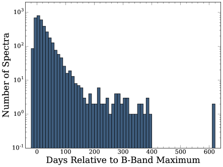
Figure 4: Histogram of the number of individual SN spectra at each epoch in the nominal sample.

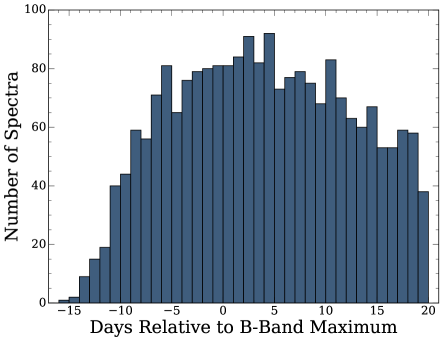
Figure 5: Histogram of the number of individual SN spectra at each epoch within 20 days of maximum brightness in the nominal sample.

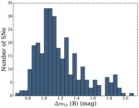
Figure 6: Histogram of the number of SNe Ia per $\Delta m_{15}(B)$ bin. This distribution is skewed towards slower-declining events and peaks at $\Delta m_{15}(B)$ $=1.12$ mag (typical for normal SNe Ia.)

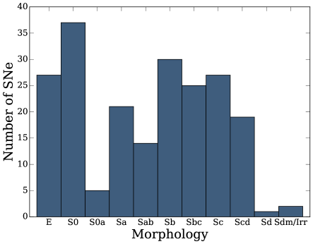
Figure 7: Histogram of the number of SNe Ia per bin in host galaxy morphology.

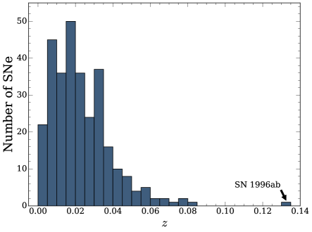
Figure 8: Histogram of the number of SNe Ia per redshift bin.

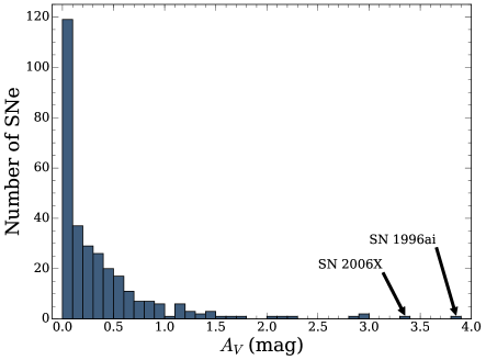
Figure 9: Histogram of the number of SNe Ia per host-galaxy extinction bin.

Some of the characteristics of the nominal sample are shown in Figures 3 $-$ 9. All SNe in the sample are at low-redshift (median $z=0.02$), vary greatly in their light-curve shapes ($0.68\leq$ $\Delta m_{15}(B)$ $\leq 2.09$ mag), and occur in a diversity of host environments. For SNe Ia without an explicit measurement of $\Delta m_{15}(B)$, we estimate $\Delta m_{15}(B)$ based on its power-law relationships with SALT, SALT2 and MLCS31 shape parameters (Figure 10). $s$, $x_{1}$, and $\Delta$ are taken from tables 1, 2, and 3 of Hicken et al. 2009. We also include $\Delta$ estimates from another set of MLCS fits using $R_{V}=2.5$ (Jha et al., 2007). For SNe that have been fit by more than one of these methods, we determine $\Delta m_{15}(B)$ from the power-law relationship with the lowest on outlier fraction and RMS uncertainty. Using a consistent sample of 85 SNe among fitting methods, we estimate the outlier fractions of SALT, SALT2, MLCS31, and MLCS25 to be 0.082, 0.035, 0.024, and 0.071 respectively, and the RMS uncertainties to be 0.071, 0.066, 0.070, and 0.074 respectively. Thus, we choose to give MLCS31 highest priority, followed by SALT2, SALT, and then MLCS25 for determining $\Delta m_{15}(B)$ from a given light-curve shape parameter.

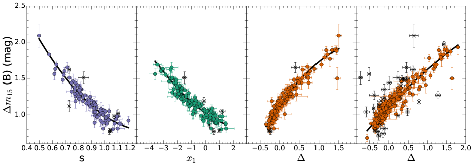
Figure 10: Power-law relationships between $\Delta m_{15}(B)$ and the light-curve shape parameters $s$ (SALT; first), $x_{1}$ (SALT2; second), $\Delta$ (MLCS using $R_{V}=3.1$; third), and $\Delta$ (MLCS using $R_{V}=2.5$; fourth). We use these relationships to determine an estimate of $\Delta m_{15}(B)$ when there is no explicit measurement available. In all panels, points marked with a black “x” are $3$-$\sigma$ outliers and are not included when fitting the relation.

3 Data Homogenization

The heterogeneous nature of spectral observations and reduction techniques has been a significant barrier to studying the bulk properties of SN Ia spectra across multiple sources. We have developed a framework to process SN spectra in order to facilitate analyses of large data sets. Prior to storing a spectrum in the database, several steps are taken to ensure homogeneity. These processing steps are applied to every spectrum in the database in addition to the nominal sample.

3.1 Variance Spectrum Generation

For many spectra, we do not have a corresponding variance spectrum. We illustrate the procedure we use to generate an approximate variance spectrum in Figures 11 and 12. First, we create a smoothed spectrum using the inverse-variance Gaussian smoothing algorithm from Blondin et al. 2006. In this work, Blondin et al. 2006 define a “smoothing factor" ($d\lambda/\lambda$) that accounts for the intrinsic broadening of spectral features due to the large expansion velocities. Since our spectra vary greatly in S/N, one value of $d\lambda/\lambda$ is not sufficient to adequately smooth every spectrum. Using a sample of spectra with varying S/N, we empirically determined the best value of $d\lambda/\lambda$ for each spectrum. We fit a linear function of S/N to these data:

$$d\lambda/\lambda=\begin{cases}0.0045&S/N<2.5\\ 4.61\cdot 10^{-3}-4.52\cdot 10^{-5}*S/N&2.5\leq S/N\leq 80\\ 0.001&S/N>80\end{cases}$$

We apply constant values of $d\lambda/\lambda$ at the extremes of our S/N range to prevent over-/under-smoothing of the data. The yellow curve in Figure 11 shows a smoothed spectrum of SN 2005lz using this method. We then subtract the smoothed spectrum from the original spectrum (blue curve), take the absolute value, and smooth again using $d\lambda/\lambda=0.015$ (orange curve in Figure 12). We account for possible uncertainty from sky emission by scaling a template sky emission spectrum to to our smoothed absolute residual spectrum, multiplying by a constant factor, and adding this to our smoothed absolute residual spectrum. We chose a value for the constant factor that provides a reasonable match to the uncertainty due to sky emission seen in the CfA spectra.

We compare the generated approximate uncertainty spectra to the associated uncertainty spectra of the CfA sample. We find that we consistently underestimate the uncertainty of the CfA sample at bluer wavelengths (see Figure 12). To quantify this effect, we divide every CfA uncertainty spectrum by the uncertainty spectrum that we generate from the flux. We then fit a linear function of wavelength to each of these ratio spectra. For spectra without archival uncertainty spectra, we apply the mean fit as a wavelength-dependent scaling to each uncertainty spectrum in order to account for this discrepancy. After making this scaling correction, we obtain an uncertainty spectrum (pink curve) that closely matches the CfA uncertainty spectrum (green curve), especially at bluer wavelengths.

3.2 Removal of Residual Sky Lines, Cosmic Rays, and Galaxy Emission Lines

We attempt to remove any residual night sky lines, cosmic ray hits, and host-galaxy emission lines that are still present. We generate a smoothed absolute residual spectrum via the same method in Section 3.1. We interpolate the flux and the variance over regions where the residual spectrum exceeds this smoothed residual spectrum by ${>}5\sigma$, where $\sigma$ is the local scatter obtained from the variance spectrum. We also increase the threshold for clipping of negative residuals to $10\sigma$ in regions where absorption lines from Ca H&K, Na I D, K 1 $\lambda 7687$, and the 5780 Å diffuse interstellar band may exist. The effects of this method are shown in Figure 11. The narrow emission features (red) have been removed resulting in the blue curve.

3.3 Reddening Corrections, Deredshifting, and Re-binning

We correct each flux and variance spectrum for MW-reddening using the Schlafly and Finkbeiner reddening map (Schlafly & Finkbeiner, 2011), a Fitzpatrick 1999 (F99) reddening law, and $R_{V}=3.1$. We then deredshift the spectrum, rebin at equally spaced wavelength values ($\Delta\lambda=2$ Å) using a flux-conserving interpolation algorithm, and store the re-binned spectrum in the database. Since interpolation introduces unwanted correlation in our variance spectra, we scale our original variance spectrum to the rebinned variance spectrum. When available, we use MLCS reddening parameters to correct for the distortion introduced by host-galaxy reddening. Since there is a larger degree of uncertainty associated with this step, the non-corrected spectra are stored in the database and we perform this correction during our analysis.

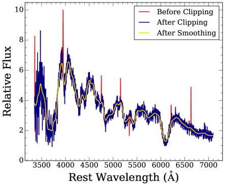
Figure 11: Spectra SN 2005lz before (red curve) and after (blue curve) removing unwanted features using the method described in section 3.2. The smoothed spectrum (with $d\lambda/\lambda=0.004$; yellow curve) is used to estimate a preliminary uncertainty in order to determine the clipping threshold.

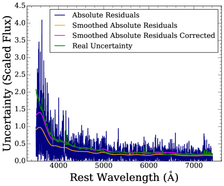
Figure 12: Uncertainty spectra corresponding to the spectrum of SN 2005lz presented in Figure 11. The blue curve is the absolute residual spectrum from the difference between the clipped spectrum and the smoothed spectrum, the green curve is the real uncertainty spectrum from the CfA archive, the yellow curve is the smoothed absolute residual spectrum, and the pink curve is the same spectrum after applying a small scaling in order to better match the green curve.

4 Generating Composite Spectra

The large sample necessitates a reliable way to visualize and validate the data and our processing techniques. Composite spectra provide a reasonable solution to this problem. They attempt to provide the “most representative” average of a given subset of data. We use this tool to reproduce the known spectral trends in SNe Ia in order to verify that our sample is of high quality. By maximizing S/N and reducing the impact of outliers, composite spectra make it easy to analyze the differences between complex spectral feature shapes. This is an advantage over measurements of derived quantities from individual spectra like velocities, EWs, and line ratios, which significantly reduce the available information and may only apply to a subset of the data (e.g., not all spectra have obvious carbon absorption).

We show that composite spectra in combination with relational queries with kaepora provide for a fast means of validating known relationships and testing different hypotheses. We always find it useful to follow up potential trends seen in composite spectra with an analysis of the individual underlying spectra.

Here we describe our method for generating composite spectra from subsets of our nominal sample. The basic algorithm is adapted from the methods used in Foley et al. 2008a and Foley et al. 2012. Reference these works for a more detailed description of the potential systematic errors introduced using these techniques. We require $A_{V}<2$ for each SN included in the composite spectra generated for this work.

4.1 Algorithm

When combining spectra from a subsample of SNe, we make an effort to ensure that the selected sample of SNe are representative of their respective populations. Multiple spectra from a single SN may satisfy a given query and in this case, we first create individual inverse-variance weighted composite spectra for each of these SNe using the methods described below. If a spectrum does not overlap with any other spectra from the same SN we attempt to add it in during the next step (if there is still no overlap, the spectrum is ignored). Once the set of spectra (now including combined spectra) is selected, we scale the flux of all spectra to the flux of the spectrum with the largest wavelength range (the preliminary template spectrum) by minimizing the sum over wavelength of the absolute differences between each spectrum and this template spectrum. A new template spectrum is then created by averaging these spectra weighted by their inverse variance (or taking the median). Spectra in the original sample that did not have overlap with the largest wavelength spectrum may potentially overlap with this new template spectrum. This process is repeated until all possible spectra are included in the composite spectrum. The $50$ Å at the beginning and end of each spectrum are ignored when constructing composite spectra in order to suppress any systematic errors that frequently occur in these regions.

It is often the case that one or a few high-S/N spectra will strongly influence the overall continuum and spectral features of the composite spectrum. This is a larger problem for smaller sample sizes where the median may be a more appropriate representation of the underlying spectra. Highly unequal weight distributions also tend to cause discontinuities in the composite spectrum at wavelengths where highly weighted spectra end. These issues can be resolved by assigning equal weights to each spectrum at the expense of S/N of the composite spectrum. We re-weight using Gini coefficients to mitigate this issue. This solution is a middle-ground approach that avoids discontinuities while attempting to still maximize S/N.

In this case, the Gini coefficient is used to measure how much the distribution of weight deviates from complete equality. It ranges from 0 to 1, where 0 means complete equality and 1 means complete inequality. Therefore in the context of combining spectra, a Gini coefficient of 0 indicates equal weight given to each spectrum (i.e., the average) and a gini coefficient of 1 indicates that a single spectrum carries all of the weight. Equation 1 defines the Gini coefficient as half of the relative mean absolute difference. For our purposes, $w_{i}$ represents the total weight (sum of inverse variance) given to an individual spectrum in some wavelength range, and $N$ is the number of spectra contributing to the composite spectrum in that same wavelength range.

$$G=\frac{\sum\limits_{i=1}^{N}\sum\limits_{j=1}^{N}|w_{i}-w_{j}|}{2N\sum\limits_{i=1}^{N}w_{i}}$$ (1)

We separate the composite spectrum into $1000$ Å regions and measure $G$. If $G>0.6$ in any of these wavelength bins, we subsequently de-weight the individual spectrum that carries the most weight across its whole wavelength range by a constant factor. This process is iterated until $G<0.6$ in all wavelength bins. We chose a value of $G<0.6$ as our threshold because it tends to provide a reasonable compromise between the average and the inverse-variance weighted average. This method allows us to achieve better S/N in our composite spectrum than the average without a strong bias towards the highest S/N spectra. This tends to result in a smooth composite spectrum that is more representative of the underlying data.

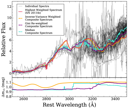
Figure 13: (top panel): Composite spectra generated from a subsample (black curves) using different methods. The red dashed curve is a high S/N spectrum of SN 2011fe. This spectrum carries the most weight in this wavelength range. The cyan curve is the median composite spectrum, the yellow curve is the inverse-variance weighted composite spectrum, and the purple curve is the Gini-weighted composite spectrum. The Gini-weighted composite spectrum is less influenced by SN 2011fe than the inverse-variance weighted composite spectrum while maintaining a larger S/N that the median composite spectrum. (bottom panel): The average value of $\Delta m_{15}(B)$ as a function of wavelength for each composite spectrum.

We demonstrate the effects using different methods to construct composite spectra in Figure 13. Here we have generated composite spectra from a sample of 180 spectra of 82 total SNe. These spectra have phase between $-4$ and $0$ days and $\Delta m_{15}(B)$ $<1.25$ mag. The black curves are individual spectra (or combined spectra from the same SN) of varying S/N, the red dashed curve is a high-S/N spectrum SN 2011fe, and the other colored curves are composite spectra generate from these individual spectra using three different methods; medianed (cyan), inverse-variance weighted (yellow), and “Gini-weighted" (purple). As expected, the inverse-variance weighted composite spectrum (yellow curve) is strongly influenced by the high S/N spectrum of SN 2011fe. We find that the median composite spectrum works well in this wavelength range and the Gini-weighted composite spectrum is consistent with the median, but with higher S/N. We also see that as $N$ increases, the properties of the Gini-weighted composite spectrum approach the inverse-variance weighted composite spectrum. The average gini coefficients of the inverse-weighted composite spectrum and the Gini-weighted composite spectrum in this wavelength range are 0.86 and 0.57 respectively. The effective value of $\Delta m_{15}(B)$ for our Gini-weighted composite spectrum is consistent with the median at wavelengths ${<}2950$ Å and then smoothly approaches the inverse-variance weighted value as $N$ increases. This is expected since SN 2011fe carries less overall weight as more spectra contribute to each weighted composite spectrum. Since we have demonstrated that Gini-weighted composite spectra are more reliable for sample sizes that vary with wavelength, the composite spectra presented in this work are constructed using this method unless specified otherwise.

4.2 Uncertainty of Composite Spectra

To understand the subtle differences between composite spectra we need an estimate of the uncertainty at each wavelength. We implement a bootstrap resampling with replacement algorithm in order to estimate the variation about the average spectrum.

Although not completely independent, the bootstrapping uncertainty is different from the root-mean-square error (RMSE) in several ways. The bootstrapping method assumes that the given sample probes the diversity of the underlying population. This diversity is manifested in the bootstrapping uncertainty by taking random resamples of the original set of spectra. This means that composite spectra with high S/N can still have large bootstrapping uncertainty if the underlying population is diverse. Therefore, the bootstrapping uncertainty provides information about the reproducibility of the average spectrum. The RMSE is typically smaller than the bootstrapping uncertainty and less affected by the diversity of the underlying population. At any given wavelength, the bootstrapping uncertainty may be estimated from the full distribution (and therefore asymmetric about the average spectrum) while the RMSE is defined as being symmetric about the average spectrum.

The uncertainty that we observe is a combination of several effects. The blue end of our composite spectra are primarily dominated by the intrinsic variation of the sample which increases towards the UV (Foley et al., 2008a), Poisson noise because we have fewer spectra contributing to the average, and the typically low detector responses in this region. We correct the continuum for host-galaxy extinction using an estimate of $A_{V}$ from an MLCS2k2 fit (Jha et al., 2007). Since we normalize our spectra by minimizing absolute differences in the overlap region with the template spectrum (see Section 4.1), we effectively normalize near $5000\$ Å on average. Therefore, spectra with anomalous continua can cause more scatter farther away from this central wavelength. Since host-galaxy extinction corrections modify the continua of our spectra, we expect that the uncertainty at the red end of a composite spectrum is dominated by imperfect corrections for reddening.

4.3 Example Composite Spectrum

In Figure 14 we present a Gini-weighted composite spectrum constructed from 142 maximum-light spectra ($-1<\tau<+1$ days, and $\Delta m_{15}(B)$ $<1.8$ mag) of 96 SNe Ia. This composite spectrum has an average phase of $0.11$ days, an average $\Delta m_{15}(B)$ $=1.11$ mag, and an average $z=0.013$. In the first panel, the blue curve is the relative flux and the blue-shaded region is the $1\sigma$ bootstrap resampling region. Our composite spectrum covers a wavelength range where we require at least 5 contributing SNe. We exclude the fastest declining events ($\Delta m_{15}(B)$ $<1.8$ mag) because there continua are often far redder than the rest of the sample. Overall, the flux and the average properties of our maximum-light composite spectrum are very similar to those of a normal SN Ia.

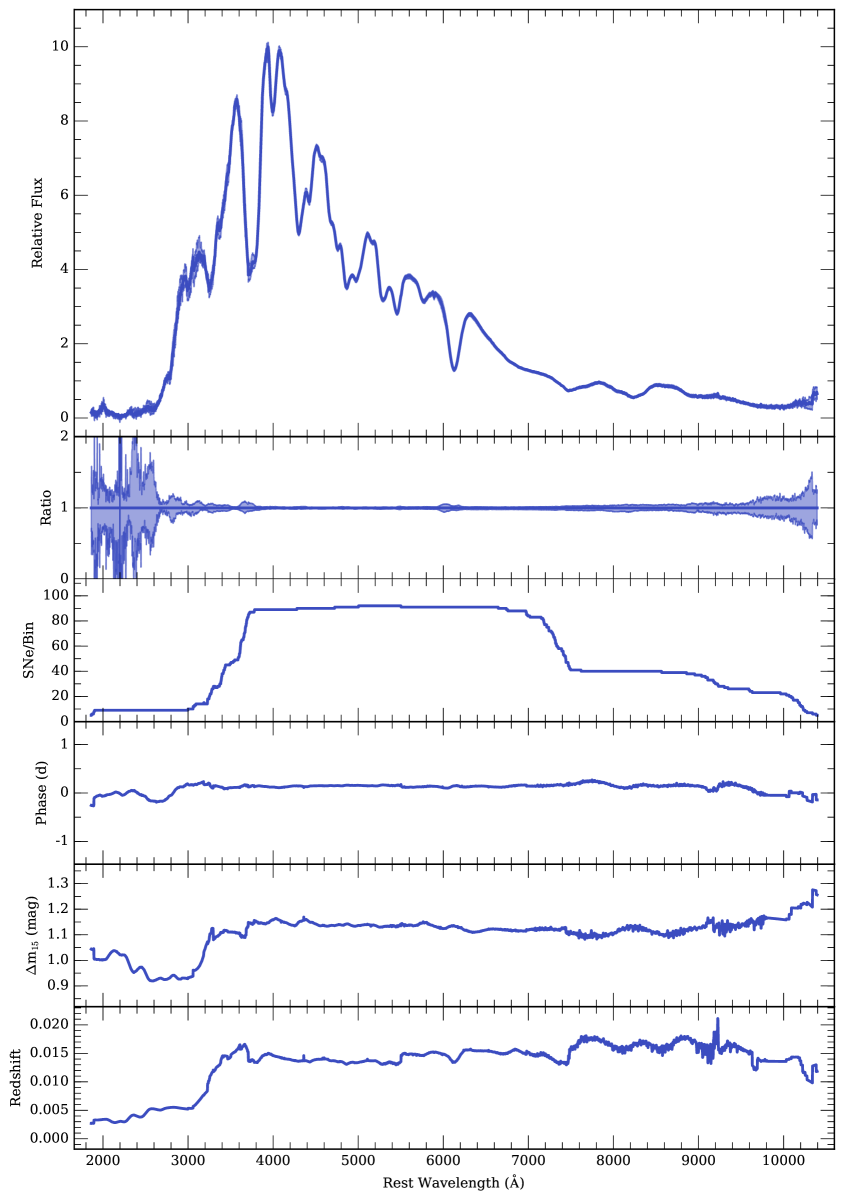
Figure 14: (first panel): Maximum-light composite spectrum created from our nominal sample consisting of spectra from 145 spectra of 96 SNe ($-1<\tau<+1$ days, and $\Delta m_{15}(B)$ $<1.8$ mag). The light-blue region is the $1\sigma$ bootstrap sampling uncertainty. (second panel): The light-blue region is the ratio of the $1\sigma$ bootstrap sampling uncertainty relative to the composite spectrum. (third panel): The number of individual spectra contributing to each wavelength bin. For this composite spectrum, a minimum of 5 and a maximum of 96 spectra contribute at any given wavelength. (fourth panel): The average phase relative to maximum brightness as a function of wavelength for this composite spectrum. (fifth panel): The average value of $\Delta m_{15}(B)$ as a function of wavelength for this composite spectrum. (sixth panel): The average redshift of the composite spectrum as a function of wavelength.

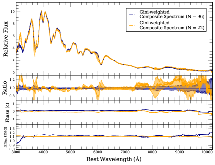
Figure 15: (first panel): The maximum-light composite spectrum from Figure 14 (blue curve) compared to a maximum-light composite spectrum constructed from a subsample of 15 SNe Ia with $-1<\tau<+1$ days and $1.05<$$\Delta m_{15}(B)$ $<1.15$ mag (yellow curve). The shaded regions are the $1\sigma$ bootstrap sampling uncertainties of the respective composite spectra. (second panel): The ratio of the given composite spectra and $1\sigma$ bootstrap sampling regions to the larger sample size composite spectrum. (third panel): The average phase relative to maximum brightness as a function of wavelength for a given composite spectrum. (fourth panel): The average value of $\Delta m_{15}(B)$ as a function of wavelength for a given composite spectrum.

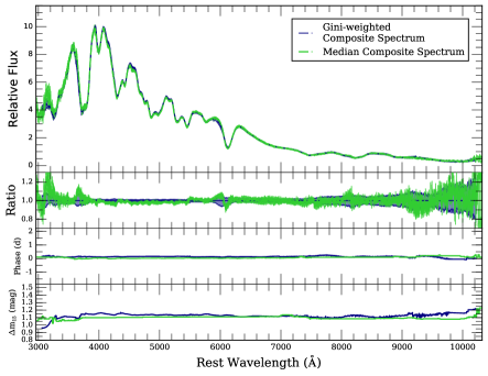
Figure 16: A comparison between Gini-weighted composite spectra and median composite spectra constructed from the subsample of 96 SNe Ia with $-1<\tau<+1$ days and $\Delta m_{15}(B)$ $<1.8$ mag (blue and green curves respectively). The panel format is the same as Figure 15.

The second panel contains the $1\sigma$ bootstrap contours divided by the relative flux of the composite spectrum. This fractional uncertainty is largest below $3200$ Å. The uncertainty also gradually increases redward of ${\sim}6000$ Å. The fractional uncertainty is smallest between these regions because this is both the region where most spectra overlap, and the region where most spectra are effectively normalized. There is a slight correlation of the fractional uncertainty with the Si II and Ca II absorption features. This correlation is likely caused by the variability of line velocities in the underlying sample.

Since the wavelength ranges of individual spectra can vary greatly, the number of of contributing events varies with wavelength. The third panel of the figure shows the number of SNe contributing to the composite spectrum as a function of wavelength. Since the CfA could obtain spectra frequently, it is more likely that to have spectra within a small phase window than other surveys. Therefore, a large portion of this subsample are spectra obtained with the FAST spectrograph. This instrument has a wavelength coverage of ${\sim}3700-7600$ Å (Fabricant et al., 1998). Thus the number of spectra contributing to the composite spectrum reaches its maximum in this wavelength range.

Additionally, since the variance of individual spectra vary with wavelength, the average properties of composite spectra can change with wavelength. Panels $4-6$ of Figure 14 show the variation of phase, $\Delta m_{15}(B)$, and redshift with wavelength. There is a large shift in the average properties from the UV to the optical part of our composite spectrum. This change is due to the fact that UV spectra tend to be from intrinsically bright and nearby events. Overall, there is not much variation in these average properties in the optical, but there does seem to be some slight correlation with the stronger spectral features. It is also important to note our maximum-light composite spectrum is subject to Malmquist bias. However, analyses of subsamples with comparable $\Delta m_{15}(B)$ should not be as heavily impacted by this effect.

We find that composite spectra with similar average properties tend to look remarkably similar regardless of sample size. In Figure 15 we compare our maximum-light composite spectrum ($N$ = 96; blue curve) to a maximum-light composite spectrum constructed from a smaller sample of SNe ($N$ = 22) with the same average phase and $\Delta m_{15}(B)$ ($-1<\tau<+1$ days and $1.05<$$\Delta m_{15}(B)$ $<1.15$ mag). This composite spectrum has an average phase of $0.13$ days, an average $\Delta m_{15}(B)$ $=1.09$ mag, and an average $z=0.015$. These properties are very similar to those of the composite spectrum constructed with a larger $\Delta m_{15}(B)$ window. Most of the differences are captured by the $1\sigma$ bootstrap uncertainty regions and the largest differences occur in regions where the average light curve shapes differ between composite spectra (${\sim}3200$ Å).

We also compare these Gini-weighted maximum-light composite spectra to median composite spectra generated from the same subsamples (Figure 16). Generally, the Gini-weighted composite spectrum is very similar to the corresponding median composite spectrum at all wavelengths and has higher S/N. The small differences tend occur at the large spectral features. The most discrepant regions are the Si II and Ca II absorption features, however the differences are consistent with the $1\sigma$ bootstrap uncertainty region of the Gini-weighted composite spectrum and vice versa.

5 Results and Analysis

In this section, we use kaepora to generate subsets of our nominal sample with desirable average properties. We present composite spectra generated using our Gini-weighting method from these subsets that vary primarily with phase and light-curve shape. We demonstrate that our composite spectra reproduce known correlations between spectral and photometric properties. We obtain composite spectra with desired properties by making cuts on the certain parameter ranges. We often refer to this process as “controlling for" a specific parameter. Finally, we investigate the spectral variation of SNe Ia residing in different host-galaxy environments.

We compare our results to four sets of SN Ia template spectra and their respective color curves. The template spectra come from Nugent et al. (2002), Stern et al. (2004), Hsiao et al. (2007), Guy et al. (2007), and Foley et al. (2008a) and will be referred to as the Nugent/Nugent-91T/Nugent-91bg, Hsiao, SALT2, and Foley template spectra respectively. These template spectra were developed with different scientific goals in mind. It is also important to note that the spectral samples used in constructing these spectral templates will inevitably overlap with some of the data in our nominal sample. It is difficult to know exactly which data are shared between template spectra, but we still expect to find similar results because of this overlap.

The Nugent and Hsiao template spectra were created for the purpose of determining $K$-corrections for samples of SNe Ia. The Nugent template spectra are solely dependent on phase and use only local SNe Ia. The Nugent template spectra are heavily influenced by SNe 1989B, 1992A, and 1994D. One of which has strong dust reddening (SN 1989B; Wells et al. 1994b) and another of which has anomalous luminosity and colors (SN 1994D; Richmond et al. 1995; Patat et al. 1996b). We include the Nugent template spectra in our comparisons but acknowledge that significant discrepancies may be caused by the weight of these atypical SNe.

The Hsiao template spectra improve on the method for constructing spectral templates and provide a phase dependent spectral sequence for normal SNe Ia. The number of spectra contributing to these epochs ranges from 16 spectra at 85.6 days to 71 spectra at 0 days. Additionally, the spectral library used to construct these template spectra included a sample of high-$z$ SNe Ia. The total sample included 576 spectra of 99 SNe at $z<0.2$ and 32 spectra of 32 SNe at $z>0.2$ (Hsiao et al., 2007). While small compared to the total sample, the high-$z$ sample is restricted in phase and light-curve shape greatly influences the UV region of the Hsiao template spectra. The colors of the Hsiao template spectra are set to match the B-band template light curve from Goldhaber et al. (2001) and the UVR-band template light curves from Knop et al. (2003).

SALT2 was developed to improve distance estimates of SNe Ia. This light-curve fitter models the evolution of the mean spectral energy distribution (SED) of SNe Ia along with its variation with light-curve shape and color (Guy et al., 2007). We are interested in improving our understanding of this multi-dimensional spectral surface with our composite spectra. The SALT2 model also makes use of high-$z$ SN data in order to constrain the UV continuum. In the sections below we compare the properties of our composite spectra to version 2.4 of the SALT2 spectral sequence model.

The Foley template spectra were created to investigate the potential evolution of SNe Ia with redshift. The methods for constructing our composite spectra are similar to this work and make use of inverse-variance weighting to produce composite spectra. These composite spectra vary with phase, light-curve shape, and redshift.

5.1 Evolution of Phase-binned Composite Spectra

We first examine the spectral evolution of our composite spectra. In Figure 17, we present 62 phase-binned composite spectra with phase ranging from $-11.2$ to $+270.5$ days. This set of composite spectra represents all of the spectra in our nominal sample. The time of maximum light of each SN is likely the largest source of error on phase (typical uncertainty $0.5$ days), therefore we do not assume that our composite spectra can differentiate spectral features with sub-day precision. We require a minimum bin size of 1 day and expand the size of the phase bin as needed as we probe later epochs. We require a minimum of 20 individual SNe per composite spectrum. We also require at least 5 spectra per wavelength bin and thus these composite spectra have differing wavelength ranges. For clarity, the $1\sigma$ bootstrap uncertainty regions and other composite spectrum properties are are not displayed. However, each of these composite spectra can be decomposed in a similar way to our maximum-light composite spectrum in Figure 14.

The spectral features evolve smoothly with time and clearly show how the average SN Ia transitions from its photospheric phase, dominated by absorption from intermediate mass elements (IMEs), to the nebular phase, which is dominated by forbidden emission from iron-group elements (IGEs). There is a slight tendency to see small discontinuities near the edges of the composite spectra where $N$ is small and near ${\sim}7600$ Å (the red end of the CfA sample’s wavelength coverage). The overall effect on the continuum is small and most often captured by the bootstrapping uncertainty region. Our composite spectra are comprised of spectra coming from a diversity of events, therefore, at any specific phase normal selection biases will apply. In particular, composite spectra for later phases are more likely to be influenced by intrinsically bright events.

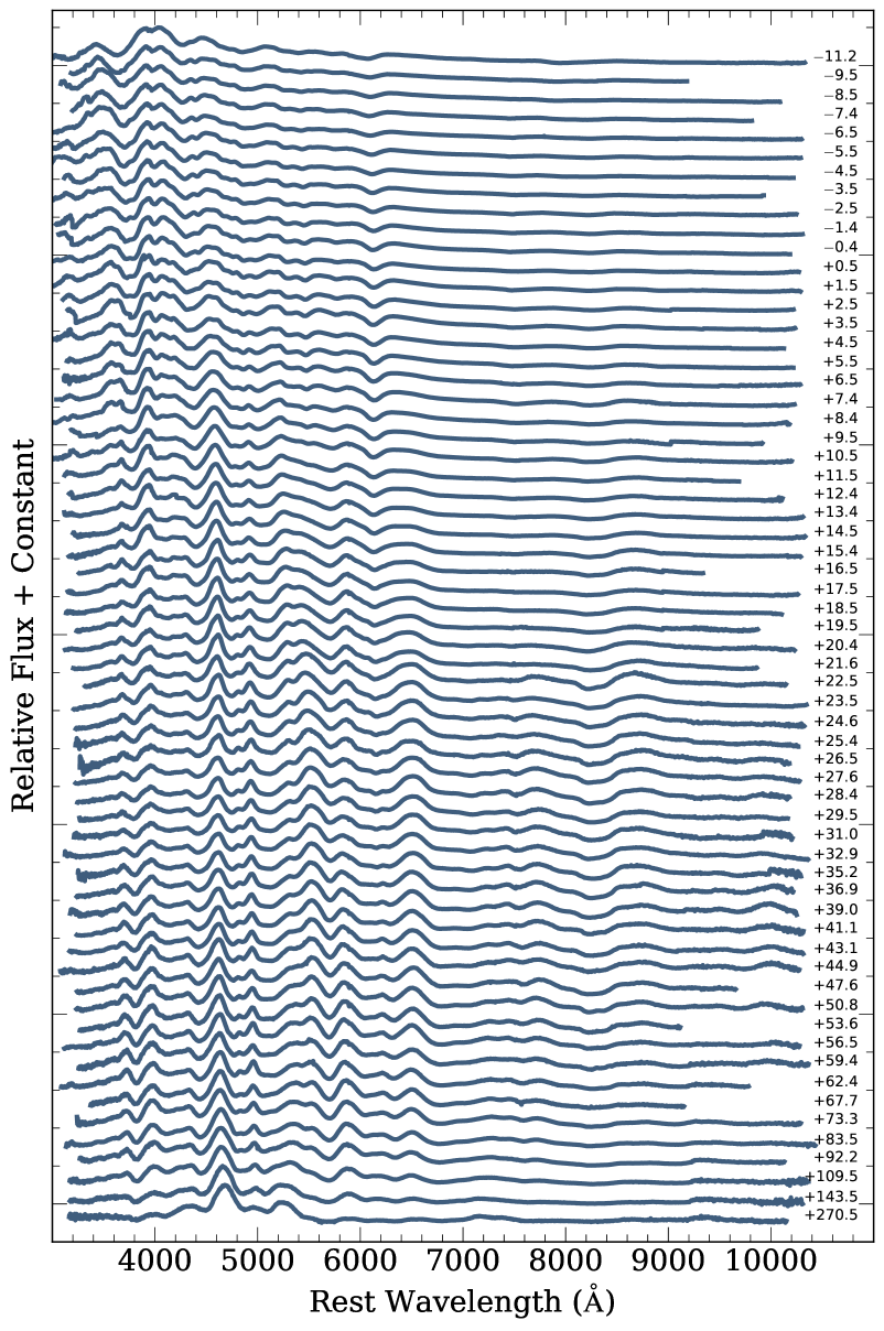
Figure 17: Composite spectra generated from the nominal sample showing the time evolution of spectral features of SNe Ia. A time series is plotted with effective phases of $t=-11.3$ to $t=271.2$ days relative to $B$ maximum brightness. Minimum bin sizes of 1 day are enforced near maximum brightness. Bin sizes are adjusted accordingly at later epochs to include a statistically significant ($N\geq 20$) sample for each composite spectrum.

In Figure 18, we present 16 phase-binned composite spectra ranging from $-11$ days relative to maximum light to $16$ days after maximum light using a bin size of 2 days. The Si II and Ca II absorption features evolve smoothly with time indicating a steady change in photospheric velocity. The minima of these features progress towards redder wavelengths indicating a smooth decrease in velocity with time.

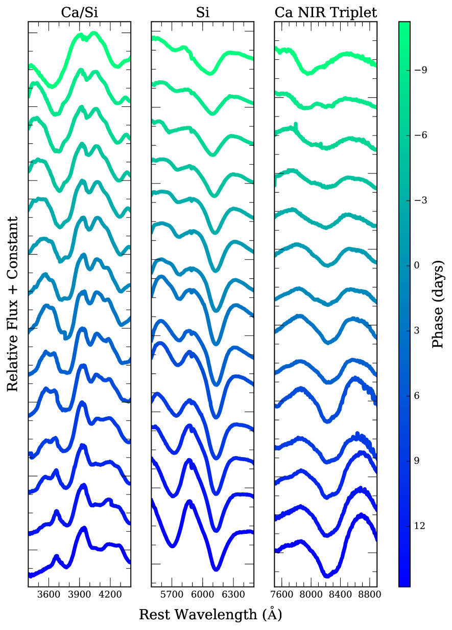
Figure 18: Zoomed-in composite spectra within 16 days of maximum light created from the nominal sample. The spectral absorption features associated with Ca II H$\&$K, Si II, and the Ca II NIR triplet are shown in the left, middle and right panels respectively. Bin sizes of 2 days are used for each of these composite spectra.

Beyond MW and host galaxy extinction corrections, we do not make any modifications to the continua of our composite spectra. The $B-V$ color evolution of these composite spectra is very similar to that of normal SNe Ia. This similarity means that the relative flux calibration among different surveys is good enough to produce reliable mean continua.

In Figure 19, we show the $B-V$ color evolution of our composite spectra with $\Delta m_{15}(B)$ $<1.8$ mag (red squares) and compare to the Nugent (cyan), Hsiao (yellow), and SALT2 template spectra (black) for phases ranging from $-12$ to $+56$ days. We also investigate the effects of binning our composite spectra with $1.05\leq$ $\Delta m_{15}(B)$ $\leq 1.25$ mag (dark blue stars). We chose this bin size for $\Delta m_{15}(B)$ since the Hsiao and Nugent template spectra were created to represent $s=1.0$ ($\Delta m_{15}(B)$ $\approx 1.1$ mag) SNe, and the SALT2 base template spectrum has $x_{1}=0$ ($\Delta m_{15}(B)$ $\approx 1.1$ mag). Thus our sets of composite spectra with large and small $\Delta m_{15}(B)$ windows have average values of $\Delta m_{15}(B)$ that range from $1.03-1.17$ mag and $1.07-1.11$ mag respectively. This means that on average these two sets of composite spectra have very similar light curve shapes.

Overall, we see good agreement with the the three template spectra. We also find that our two sets of composite spectra with different $\Delta m_{15}(B)$ windows are consistent at all phases. This further reinforces the fact our composite spectra with larger sample sizes (due to having larger ranges of light curve shape) are representative of SNe Ia with the average properties of our underlying samples. On average, our composite spectra are most consistent with Hsiao and slightly bluer than the SALT2 and Nugent color curves. The slope of the Nugent template spectrum between the epochs of $-6$ and +24 days is significantly larger than the other color curves. This difference may be due to the influence of atypical SNe on the Nugent template spectrum. Both the Hsiao and Nugent spectral templates are warped to match the photometry of template light curves in the literature (Hsiao; $B$-band Goldhaber et al. 2001, $UVR$-band Knop et al. 2003, Nugent; $B$-band Riess et al. 1999, $RI$-band Knop et al. 2003). Our composite spectra reproduce a normal SN Ia $B-V$ color curve without the need for spectral warping and thus preserve absorption features, lines ratios, and velocities that are representative of the underlying spectra.

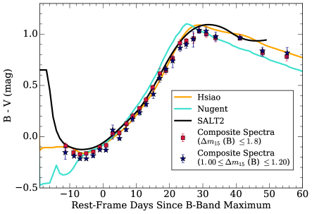
Figure 19: Comparison of the $B-V$ color evolution of various SN Ia template spectra and our composite spectra created from the nominal sample. The orange, light-blue, and black curves are the Hsiao, Nugent, and SALT2 template spectra respectively. The red squares are color measurements from composite spectra generated from the nominal sample with $\Delta m_{15}(B)$ $<1.8$ mag. The blue stars are color measurements from composite spectra generated from the nominal sample using only SNe where $1.00\leq$ $\Delta m_{15}(B)$ $\leq 1.20$ mag. Bin sizes of 2 days are used for phase $\leq$+30 days and bin sizes of 4 days are used for phase $>$+30 days.

Si II $\lambda 6355$ line velocities measured from these composite spectra are also representative of their respective subsets. In Figure 20, we compare the velocity evolution of our composite spectra (black) to the distributions of velocities of the individual SNe in each phase bin (distinguished by color) covering phases between $-13$ and $+16$ days. We also compare to the velocity evolution of the median velocity measurement in each phase range (brown), and median composite spectra generated from the same subsets (orange).

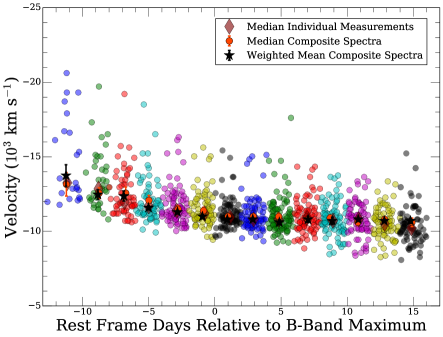
Figure 20: Velocity evolution of our composite spectra created from the nominal sample. Black stars are measurements from the weighted mean composite spectra and orange circles are measurements from median composite spectra. The smaller circle points are measurements from the individual spectra. These are color coded to distinguish the borders of the phase bins defined for the composite spectra. The brown diamonds correspond to the median of the individual measurements within each bin.

The velocities of our composite spectra are consistent with these measurements across all phases and range from a blueshift of $-13{,}700$ km s^-1 at -11 days to $-10{,}700$ km s^-1 at +15 days. The velocities of our weighted mean and median composite spectra steadily decline with phase until around maximum light where they level off at $\sim$ $-10{,}800$ km s^-1. Due to the lack of data at very early epochs (${<}-10$ days), it is likely that the velocity of our composite spectrum is slightly underestimated at this phase.

5.2 Maximum-Light $\Delta m_{15}(B)$-binned spectra

We also examine luminosity-dependent spectral differences through the light-curve decline rate parameter $\Delta m_{15}(B)$ for events near maximum light. In Figure 21 we present 6 maximum light composite spectra where we have controlled for light-curve shape. Here we expand our phase range to include spectra with phase between $-$3 and +3 days. We require at least 5 spectra per wavelength bin which results in varying wavelength ranges among the composite spectra. Since there are more UV spectra for slow-declining events that tend to have higher luminosities, we are able to extend two of these composite spectra into the UV.

This subdivision by $\Delta m_{15}(B)$ clearly demonstrates several known spectral sequences with light-curve shape. In particular the continua become redder with narrower light-curves (larger $\Delta m_{15}(B)$). We also see clear evidence of Ti II absorption at ${\sim}4300$ Å in the lowest luminosity composite spectrum ($\Delta m_{15}(B)$ $=1.87$ mag). This is a characteristic feature of the SN 1991bg-like subclass of SNe Ia (Filippenko et al., 1992a; Leibundgut et al., 1993) and is expected for these faster declining events. This composite spectrum also has stronger O I $\lambda 7773$ and Ca near-IR triplet absorption than the other composite spectra.

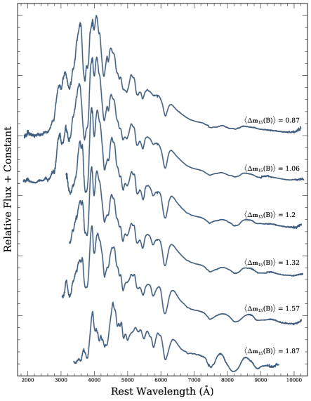
Figure 21: $\Delta m_{15}(B)$-binned maximum-light composite spectra. From top to bottom the spectra has $\Delta m_{15}(B)$ bins of $\Delta m_{15}(B)$ $<0.95$ mag, $0.95<$ $\Delta m_{15}(B)$ $<1.15$ mag, $1.15<$ $\Delta m_{15}(B)$ $<1.25$ mag, $1.25<$ $\Delta m_{15}(B)$ $<1.42$ mag, $1.42<$ $\Delta m_{15}(B)$ $<1.7$ mag, and $\Delta m_{15}(B)$ $>1.7$ mag. Phase bins of $-3<\tau<+3$ days were used for each composite spectrum. The composite spectra consist of 30, 61, 16, 23, 21, and 13 individual SNe respectively.

The average $\Delta m_{15}(B)$ for each composite spectrum is shown above each spectrum.

We measure the $B-V$ colors of our composite spectra from Figure 21 and present them in Figure 22 (blue stars). For comparison, we show measurements made from maximum-light SALT2 template spectra with effective $\Delta m_{15}(B)$ corresponding to the mean values of $\Delta m_{15}(B)$ from our composite spectra (black circles), a linear fit of this relationship from Phillips et al. (1999) (green curve), and the relationship that is produced by the MLCS2k2 model (Jha et al. 2007; orange curve).

While the SALT2 spectral feature strengths differ greatly, the $B-V$ colors of the SALT2 maximum-light spectra, by design, do not vary much with light-curve shape. The $B-V$ colors of our maximum-light composite spectra slowly become redder with $\Delta m_{15}(B)$ and then change dramatically for the fastest-declining SNe. Our composite spectra are consistent with with Phillips et al. (1999) for the slower-declining SNe Ia and produce the same general trend seen in MLCS2k2. This is not surprising because we rely on an estimate of $A_{V}$ from MLCS light-curve fits in order to correct individual spectra for host-galaxy extinction.

Figure 23 highlights the subtle differences between the Si II $\lambda 5972$ and $\lambda 6355$ absorption features of $\Delta m_{15}(B)$-binned composite spectra. Here the continuum difference between these composite spectra is obvious. Since intrinsically bright SNe tend to have bluer colors, our composite spectra progress towards having redder continua as the average light-curve shape becomes narrower ($\Delta m_{15}(B)$ increases). Additionally, we see evidence of Na I D absorption in all composite spectra except the two with the largest effective $\Delta m_{15}(B)$ values. This trend is likely because fast-declining SNe Ia tend to occur in early-type environments devoid of gas (Hamuy et al., 2000; Howell, 2001).

From the slowest-declining to fastest-declining composite spectra (top to bottom in Figure 21) the Si II $\lambda 6355$ line velocities of these composite spectra are $-10{,}500$, $-11{,}000$, $-10{,}800$, $-11{,}200$, $-11{,}200$, and $-10{,}500$ km s^-1. These measurements are consistent with the lack of an observed correlation between light-curve shape and velocity for the bulk of SNe Ia and the tendency for events with extremely high or low values of $\Delta m_{15}(B)$ to have slightly lower velocities (Wang et al., 2009b).

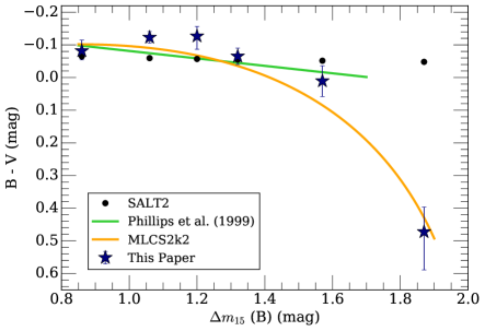
Figure 22: The relationship between $\Delta m_{15}(B)$ and $B-V$ color at maximum-light. The blue stars are measurement made from our composite spectra in Figure 21. The black circles are measurements made from maximum-light SALT2 template spectra with effective $\Delta m_{15}(B)$ corresponding to the mean values of $\Delta m_{15}(B)$ from our composite spectra. The green and orange curves are fits from Phillips et al. (1999) and Phillips (1993) respectively.

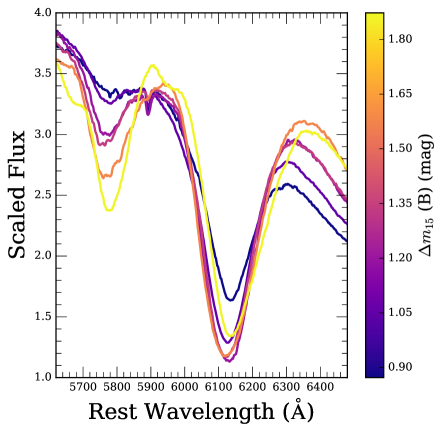
Figure 23: The Si II $\lambda 5972$ and $\lambda 6355$ absorption features of our maximum-light composite spectra from Figure 21. The color bar ranges from slow-declining light-curve shapes ($\Delta m_{15}(B)$ = 0.86 mag; dark purple) to fast-declining light-curve shapes ($\Delta m_{15}(B)$ = 1.87 mag; yellow).

In addition, the ratio of the depth of the two main Silicon absorption features ($\mathcal{R}$(Si II)) changes with light-curve shape. This sequence, originally discovered by Nugent et al. (1995), results from the changing abundance of the ionization species of Silicon (Hachinger et al., 2008). Using a similar approach to our analysis of velocity near maximum light, we compare $\mathcal{R}$(Si II) from our composite spectra (black) to those measured from the individual spectra in each $\Delta m_{15}(B)$ bin (distinguished by color; Figure 24). We also compare the median $\mathcal{R}$(Si II) measurement in each $\Delta m_{15}(B)$ range (brown), and $\mathcal{R}$(Si II) measured from median composite spectra generated from the same subsets (orange). Here we clearly show that $\mathcal{R}$(Si II) of a composite spectrum is representative of its effective decline rate. The measurements of $\mathcal{R}$(Si II) reproduce the properties of their underlying subsets and are consistent with the median properties of these individual spectra.

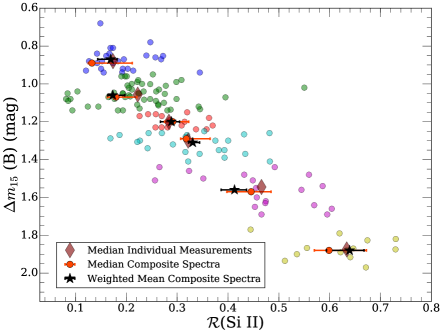
Figure 24: $\mathcal{R}$(Si II) of our $\Delta m_{15}(B)$-binned composite spectra created from the nominal sample. Black stars are measurements from the weighted mean composite spectra and orange circles are measurements from median composite spectra. The smaller circle points are measurements from the individual spectra. These are color coded to distinguish the borders of the phase bins defined for the composite spectra. The brown diamonds correspond to the median of the individual measurements within each bin.

 

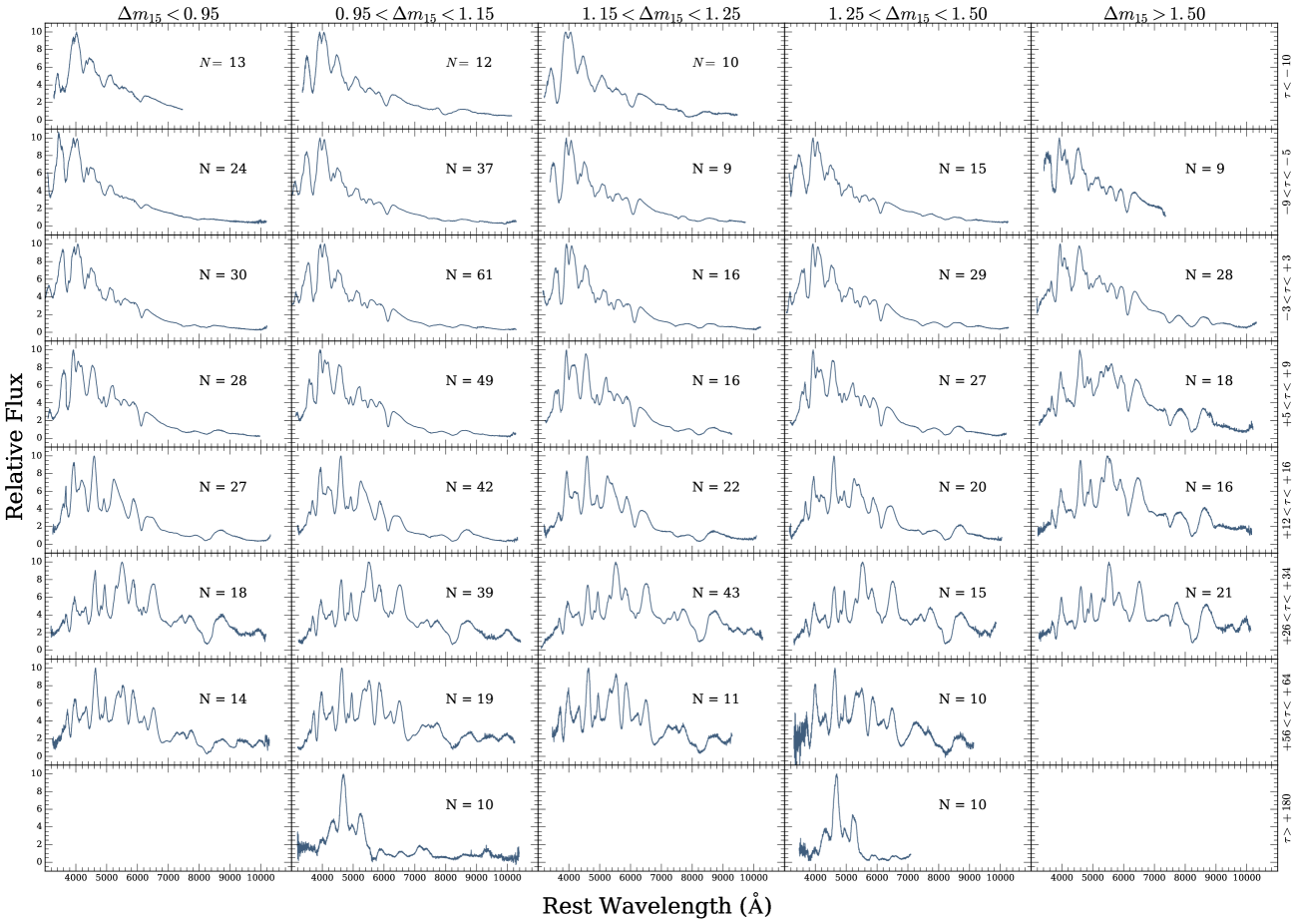
Figure 25: Phase and $\Delta m_{15}(B)$-binned composite spectra. Columns from left to right correspond to $\Delta m_{15}(B)$ bins of $\Delta m_{15}(B)$ $<0.95$ mag, $0.95<$ $\Delta m_{15}(B)$ $<1.15$ mag, $1.15<$ $\Delta m_{15}(B)$ $<1.25$ mag, $1.25<$ $\Delta m_{15}(B)$ $<1.5$ mag, and $\Delta m_{15}(B)$ $>1.5$ mag.. Rows from top to bottom corresponds to phase bins of $\tau<-10$ days, $-9<\tau<-5$ days, $-3<\tau<+3$ days, $+5<\tau<+9$ days, $+12<\tau<+16$ days, $+26<\tau<+34$ days, $+56<\tau<+64$ days, and $\tau>+180$ days. The number of individual spectra included in each composite spectrum is stated in the corresponding panel. Composite spectra have varying wavelength ranges because we require at least 5 individual spectra at any given wavelength. Blank panels correspond to regions of this parameter space where we do not currently have enough data to generate a representative composite spectrum.

The SNe in our nominal sample span a large range of light-curve shapes and their spectra cover a large range of phases. These are the primary parameters that control the spectral features of SNe Ia and we have demonstrated that our composite spectra reproduce evolution and variation with these properties. In Figure 25, we present a grid of composite spectra generated by controlling for both phase and light-curve shape. From top to bottom composite spectra are increasing in their effective phase, and from left to right composite spectra are increasing in their effective $\Delta m_{15}(B)$. So the maximum-light composite spectra from Figure 21 are represented by the third row in this grid. For clarity we have used slightly different $\Delta m_{15}(B)$ ranges and the rightmost column contains all SNe with $\Delta m_{15}(B)$ $>1.50$ mag (including SNe Ia spectroscopically similar to SN 1991bg). The amount of data contributing to each composite spectrum is related to observing strategies, intrinsic brightness, and rates. For example, the composite spectrum for bins with $-3<\tau<+3$ days and $0.95<$ $\Delta m_{15}(B)$ $<1.15$ mag contains the most individual spectra (61) likely because most SNe Ia are discovered near maximum brightness and normal SNe Ia ($\Delta m_{15}(B)$ $\approx 1.1$ mag) are relatively bright and common. Despite slower declining SNe Ia ($\Delta m_{15}(B)$ $<0.95$ mag) being intrinsically brighter, fewer spectra contribute to these composite spectra because the rates of these events are lower (Li et al., 2011). Similarly, faster declining SNe Ia ($\Delta m_{15}(B)$ $>1.50$ mag) are both intrinsically fainter and have lower rates than normal SNe Ia (Li et al., 2011). For these fast-declining events, we again see Ti II absorption at ${\sim}4300$ Å at all phases. Naturally, we also see a decrease in the number of spectra with phase as the SNe dim and get more difficult to observe.

This figure also highlights some spectral correlations that are slightly degenerate with both phase and light-curve shape. As expected, the continua of our composite spectra are bluer for earlier phases and smaller values of $\Delta m_{15}(B)$ and redder for later phases and larger values of $\Delta m_{15}(B)$. This continuum relationship is consistent with Figure 19 which shows that the $B-V$ color of our composite spectra become redder with time for phases between $-6$ and $+28$ days, and Figure 23 which also shows the tendency for maximum-light composite spectra with larger effective $\Delta m_{15}(B)$ to have redder continua. Additionally, light-curve shape and phase produce some similar effects on spectral feature strengths. For example, the strength of the Si II $\lambda 4130$ absorption feature is weaker with earlier epochs and broader light-curve shapes. The flux of the peak to the right the $\lambda 4130$ absorption feature has the tendency to decrease with phase relative to the peak to the right of the Ca H&K absorption feature. A similar correlation between these peaks exists with increasing $\Delta m_{15}(B)$ near maximum light. We also observe a slight positive correlation between $\mathcal{R}$ (Si II) and phase between $-11$ and $+9$ days. For these reasons, some composite spectra look very similar despite having very different average properties. For example, our composite spectra constructed using $-9<\tau<-5$ and $1.25<$ $\Delta m_{15}(B)$ $<1.5$ mag (row 2, column 4) and $+5<\tau<+9$ and $\Delta m_{15}(B)$ $<0.95$ mag (row 4, column 1) have similar continua and spectral feature strengths.

5.3 Template Spectrum Comparisons

In this section, we compare our composite spectra to the Nugent, Hsiao, SALT2 and Foley template spectra using various bins of phase and $\Delta m_{15}(B)$.

In Figure 26 we investigate the normal SN Ia template spectra near maximum light. We use our total maximum-light composite ($-1<\tau<+1$ days and $\Delta m_{15}(B)$ $<1.8$ mag) spectrum from Figure 14 as a comparison. Overall, our composite spectrum is most similar to the Hsiao and Foley template spectra. The majority of the Hsiao anf Foley template spectra fall within the $1\sigma$ bootstrap uncertainty of our composite spectrum and the near-UV peaks blueward of $4000$ Å are very well matched. Hsiao has slightly higher flux in some regions ${>}8000$ Å. The Nugent template spectrum is slightly bluer than the composite spectrum especially in the UV and near-UV. The SALT2 maximum-light ($x_{1}=0$) template spectrum has a slightly redder continuum than the composite spectrum and only extends from $2000-9200$  Å.

Despite the slight color differences, the relative strengths of most absorption features are very similar for our composite spectrum and the three template spectra. The Nugent template spectrum has a larger Si II $\lambda 6355$ blueshift of $-12{,}300$ km/s in comparison to our composite spectrum ($-10{,}900$ km s^-1), Hsiao ($-11{,}000$ km s^-1), Foley ($-11{,}500$ km s^-1), and SALT2 ($-11{,}300$ km s^-1).

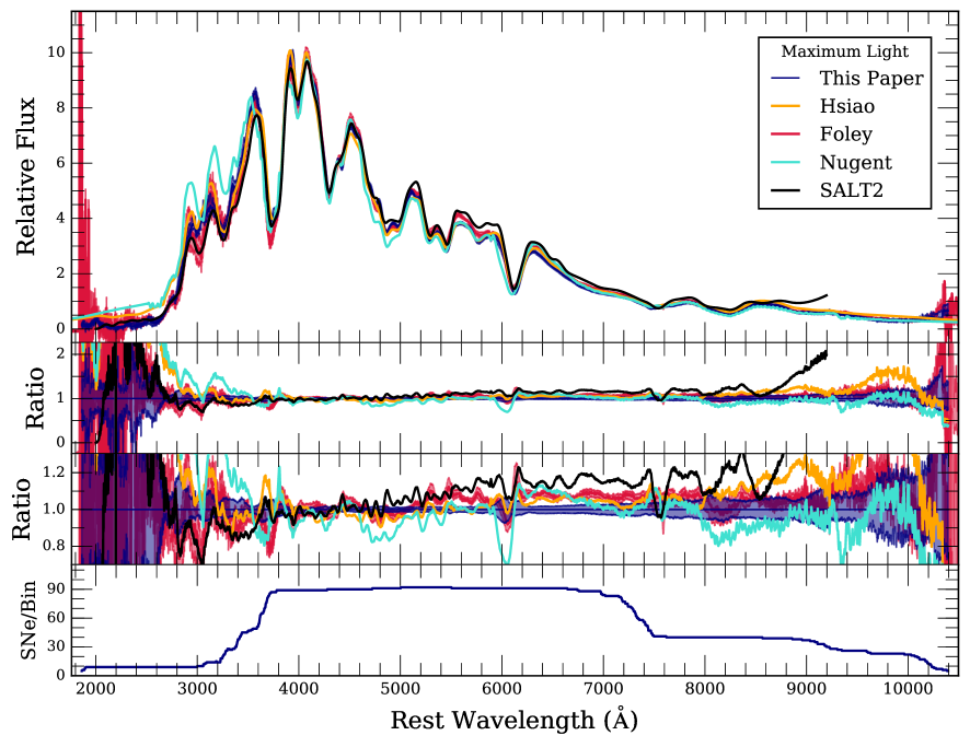
Figure 26: (first panel): Comparison of our maximum-light composite spectrum (blue curve) from Figure 14 to maximum-light template spectra from Hsiao (orange curve), Foley (red curve), Nugent (light-blue curve), and SALT2 (black curve). The blue- and red-shaded regions are the $1\sigma$ bootstrapping uncertainty on the composite spectra from this work and Foley respectively. (second panel): The ratio as a function of wavelength of a given template spectrum to our maximum-light composite spectrum. (third panel): Zoomed in version of the second panel to emphasize smaller differences between template spectra. The light-blue shaded region is the $1\sigma$ bootstrap variation of the total maximum-light composite spectrum. (fourth panel): The number of individual spectra contributing to each wavelength bin of the total maximum-light composite spectrum.

.

In section 5.1, we investigated the effect our $\Delta m_{15}(B)$ bin size on the color evolution of our composite spectra. Here we perform a similar analysis to see if spectral feature strengths differ for composite spectra with the same average properties but different sample sizes. In Figure 27 we compare our maximum-light composite spectrum with $\Delta m_{15}(B)$ $<1.8$ (blue curve) to our maximum-light composite spectrum with $1.0<$ $\Delta m_{15}(B)$ $<1.2$ mag (green curve). The latter composite spectrum was constructed from 51 spectra of 34 SNe. The differences between this composite spectrum and our maximum-light composite spectrum with $\Delta m_{15}(B)$ $<1.8$ (blue curve) are very small. There does seem to be larger variation near the stronger spectral features, but these differences are all captured by the bootstrapping uncertainty. We also see that the average phase and $\Delta m_{15}(B)$ are very similar in the wavelength range where these composite spectra overlap. For these reasons, we elect to use our composite spectra constructed from larger sample sizes when comparing to other template spectra of normal SNe Ia.

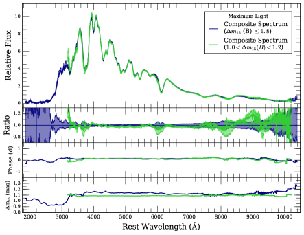
Figure 27: Same format as Figure 15 except we compare our maximum-light composite spectrum (blue curve) from Figure 26 and our maximum-light composite spectrum with $1.0<$ $\Delta m_{15}(B)$ $<1.2$ mag (green curve).

Figures 28, 29 and 30 compare our composite spectra to the Nugent, Hsiao, SALT2, and Foley template spectra at different epochs ($\sim-1$ week, $\sim+1$ week, and $\sim+1$ month respectively). The line velocities of these composite spectra are well matched by the SALT2 template spectra. We measure a Si II $\lambda 6355$ blueshift of $-12{,}600$ km s^-1 for our -1 week composite spectrum ($-11{,}700$ km s^-1, $-12{,}100$ km s^-1, $-11{,}500$ km s^-1, and $-12{,}700$ km s^-1 for the -1 week Hsiao, Foley, Nugent, and SALT2 template spectra respectively). Similarly, we measure a Si II $\lambda 6355$ blueshift of $-10{,}800$ km s^-1 for our +1 week composite spectrum ($-10{,}900$ km s^-1, $-11{,}000$ km s^-1, $-10{,}600$ km s^-1, and $-10{,}800$ km s^-1 for -1 week Hsiao, Foley, Nugent, and SALT2 template spectra respectively). At every epoch, our composite spectra best match the spectral features and continua of the Hsiao and Foley template spectra. Additionally, the SALT2 template spectra have redder continua than our composite spectra at every epoch. The largest differences tend to occur near the stronger spectral features such as Si II $\lambda 6355$ and the Ca II NIR triplet. Finally, our +1 month composite spectrum is significantly bluer than the other template spectra.

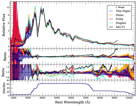
Figure 28: Same as Figure 26 except the composite spectrum (blue curve) is constructed using a phase bin of $-8<\tau<-6$ days and $\Delta m_{15}(B)$ $<1.8$ mag.

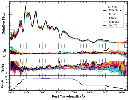
Figure 29: Same as Figure 26 except the composite spectrum (blue curve) is constructed using a phase bin of $+6<\tau<+8$ days and $\Delta m_{15}(B)$ $<1.8$ mag.

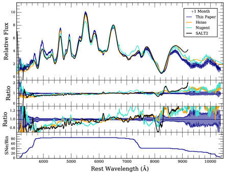
Figure 30: Same as Figure 26 except the composite spectrum (blue curve) is constructed using a phase bin of $+28<\tau<+32$ days and $\Delta m_{15}(B)$ $<1.8$ mag.

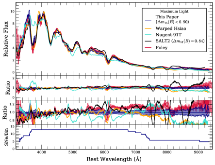
Figure 31: Same as Figure 26 except the composite spectrum (blue curve) is constructed using a phase bin of $-1<\tau<+1$ days and a $\Delta m_{15}(B)$ bin of $\Delta m_{15}(B)$ $<0.90$ mag. The maximum-light Hsiao template spectrum has been warped to match the $B$, $V$, and $R$-band photometry measured from the composite spectrum. The red curve is the Foley maximum-light, $\Delta=-0.27$ template spectrum. The light-blue is the Nugent-91T template spectrum, and the black curve is the maximum-light SALT2 model spectrum corrected for light-curve shape such that it has an effective $\Delta m_{15}(B)$ $=0.84$ mag.

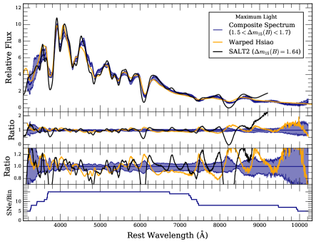
Figure 32: Same as Figure 31 except the composite spectrum (blue curve) is constructed using a phase bin of $-3<\tau<+3$ days and a $\Delta m_{15}(B)$ bin of $1.50<$ $\Delta m_{15}(B)$ $<1.70$ mag. The maximum-light SALT2 model spectrum is corrected for light-curve shape such that it has an effective $\Delta m_{15}(B)$ $=1.64$ mag.

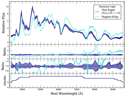
Figure 33: Comparison between a composite spectrum constructed from the fastest declining SNe Ia and the Nugent-91bg template spectrum. The composite spectrum (light-blue curve) is constructed using a phase bin of $-3<\tau<+3$ days and a $\Delta m_{15}(B)$ bin of $\Delta m_{15}(B)$ $>1.80$ mag.

We also compare SN Ia template spectra with maximum-light composite spectra for both slow and fast declining events. In Figure 31 we present our composite spectrum constructed using only slow-declining events ($\Delta m_{15}(B)$ $<0.90$ mag). For this comparison, we warp the Hsiao maximum-light ($\Delta m_{15}(B)$ $=1.1$ mag) template spectrum to match the $B$, $V$, and $R$-band photometry of the composite spectrum. We also compare to the Foley $\Delta=-0.27$ ($\Delta m_{15}(B)$ $=0.90$) template spectrum, the Nugent-91T template spectrum (Stern et al., 2004), and the SALT2 model spectrum for an event with $\Delta m_{15}(B)$ $=0.84$ mag. This value of $\Delta m_{15}(B)$ is the average $\Delta m_{15}(B)$ of our composite spectrum. The value of $x_{1}$ was chosen using the polynomial relationship between $\Delta m_{15}(B)$ and $x_{1}$ shown in Figure 10. The Si II $\lambda 6355$ feature is blueshifted $10{,}300$ km s^-1, $11{,}000$ km s^-1, $12{,}000$ km s^-1, and $10{,}700$ km s^-1 for the composite spectrum, warped Hsiao template spectrum, Foley $\Delta=-0.27$ template spectrum, and SALT2 model spectrum respectively. Overall, the Foley $\Delta=-0.27$ template spectrum and SALT2 model reproduce the Si II $\lambda 6355$ and $\lambda 5972$ absorption features the best; however, both of these template spectra have slightly redder continua than the other spectra. The Nugent-91T template spectrum is almost exclusively constructed from SN 1991T which has $\Delta m_{15}(B)$ $=0.90$ mag. The Nugent-91T template spectrum reproduces the color of the composite spectrum, but does not do well reproducing individual absorption features. This difference is because our composite spectrum was constructing using all slow-declining events, and not just those from the SN 1991T-like subclass. The Foley $\Delta=-0.27$ template spectrum and our composite spectrum are well matched towards bluer wavelengths.

Similarly, we also compare template SN Ia spectra to a composite spectrum constructed from faster-declining events (Figure 32). In this case our composite spectrum created from a $\Delta m_{15}(B)$ bin of $1.50<$ $\Delta m_{15}(B)$ $<1.70$ mag. In this comparison we also warp the maximum-light ($\Delta m_{15}(B)$ $=1.1$ mag) template spectrum to the $B$, $V$, and $R$-band photometry of the composite spectrum. The SALT2 spectrum was created to represent a SN Ia with $\Delta m_{15}(B)$ $=1.64$ mag (the average $\Delta m_{15}(B)$ of the composite spectrum). It is important to note that the SALT2 template spectrum has $x_{1}=-3.06$. Since SALT2 training sample only included SNe Ia with $\Delta m_{15}(B)$ $<1.6$ ($x_{1}>-3$)(Guy et al., 2007), we caution that the SALT2 template may not be adequately representative of these lower-luminosity SNe Ia. This SALT2 template spectrum does not match the composite spectrum as well as the slow-declining template spectrum matches the corresponding composite spectrum in Figure 31. Most of the absorption features of the faster-declining SALT2 template spectra are stronger than the respective features in the composite spectrum. However, the overall change in these features going from slow to faster declining events is similar between the composite spectra and SALT2 template spectra. Overall, after warping, the Hsiao template spectrum matches up well with our composite spectra for different values of $\Delta m_{15}(B)$. As expected, the largest differences between the Hsiao template spectra and our composite spectra occur in the features that strongly correlate with $\Delta m_{15}(B)$ (e.g., Si II and Ca II).

Finally, in Figure 33 we compare composite spectra for the fastest declining events $\Delta m_{15}(B)$ $>1.80$ mag to the Nugent-91bg template spectrum (Nugent et al., 2002). The Nugent-91bg template spectrum is constructed from SN 1991bg and SN 1999by and has telluric absorption included. Our composite spectrum has a bluer continuum and slightly larger line velocities. The composite spectrum also shows the Ti II absorption feature at ${\sim}4300$ Å characteristic of the SN 1991bg-like subclass.

5.4 Host-galaxy Morphology

In this section we investigate SN Ia spectral variations related to their host-galaxy environments. As seen above, SN Ia spectra strongly depend on phase and light-curve shape. We have shown that our composite spectra reproduce known spectral trends with these properties. Since low-luminosity SNe Ia tend to occur in early-type environments while high-luminosity SNe Ia tend to occur in late-type environments (Hamuy et al., 2000; Howell, 2001), composite spectra (for a specific epoch) generated by solely splitting the sample by host galaxy morphology will reflect this correlation. Therefore, we must control for light-curve shape in order to uncover the differences between similar SNe Ia that occur in varying environments.

We make a single cut on host galaxy morphology via its Hubble classification. Our composite spectra represent SNe Ia originating from late-type galaxies classified as Sa to Sd/Irr and early-type galaxies classified as E to S0a. If we split our nominal sample into these two subgroups, we see the expected trend that SNe residing in late-type galaxies have an average $\Delta m_{15}(B)$ $=1.10$ mag and the SNe residing in early-type galaxies have an average $\Delta m_{15}(B)$ $=1.47$ mag. Since the spectral features of our composite spectra change significantly with $\Delta m_{15}(B)$ (section 5.2), we need to choose ranges of $\Delta m_{15}(B)$ that produce composite spectra with similar average properties. Since the two populations have differing average light-curve shapes we create our composite spectra to have an effective $\Delta m_{15}(B)$ $\approx 1.3$ mag in order to incorporate the largest number of spectra. We match $\Delta m_{15}(B)$ between samples by making hard cuts on the allowed $\Delta m_{15}(B)$ ranges for each composite spectrum.

We have generated composite spectra for each host morphology subgroup at three separate epochs, $-6<\tau<0$ days (Figure 34), $0<\tau<+6$ days (Figure 35), and $+6<\tau<+11$ days (Figure 36). In each of these Figures the blue curve and shaded region are constructed from spectra of SNe Ia occuring in late-type galaxies and the red curve and shaded region are constructed from SNe Ia occuring in early-type galaxies. These Figures have similar format to Figure 14 where we presented our total maximum-light composite spectrum. The second panels show the ratio of the $1\sigma$ bootstrapping uncertainty regions relative to the late-type composite spectrum. The third panel shows the number of spectra contributing to each wavelength bin (we again require at least 5 spectra per wavelength bin). The other panels show the average values of phase, $\Delta m_{15}(B)$, and host-galaxy morphology as a function of wavelength for each composite spectrum. At all three epochs, we see evidence for stronger Na I D absorption in composite spectra representative of SNe residing in late-type galaxies which indicates more gas in the surrounding environment.

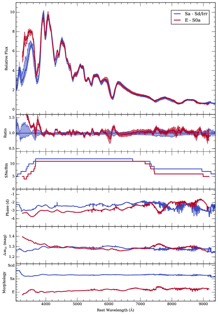
Figure 34: Same format as Figure 14 except the bottom panel now displays the average host-galaxy morphology of a given composite spectrum as a function of wavelength. The blue curves show the properties of our late-type composite spectrum and the red curves show the properties of our early-type composite spectrum. Both of these composite spectra were constructed using a phase bin of $-6<\tau<0$. The late-type composite spectrum was constructed using a light-curve shape bin of $1.20<$ $\Delta m_{15}(B)$ $<1.45$ mag. The early-type composite spectrum was constructed using a light-curve shape bin of $1.15<$ $\Delta m_{15}(B)$ $<1.50$ mag.

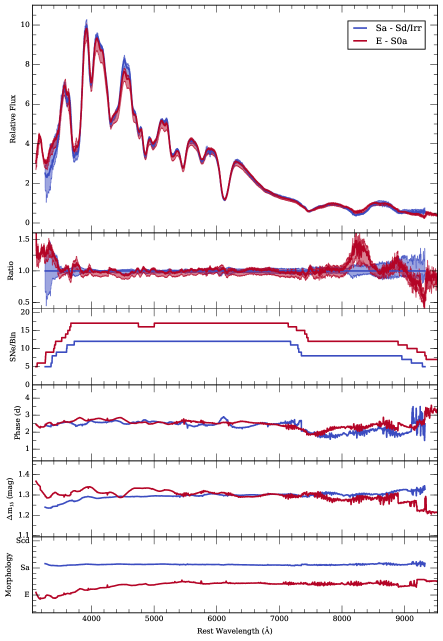
Figure 35: Same format as Figure 14. The blue curves show the properties of our late-type composite spectrum and the red curves show the properties of our early-type composite spectrum. Both of these composite spectra were constructed using a phase bin of $0<\tau<+6$. The late-type composite spectrum was constructed using a light-curve shape bin of $1.20<$ $\Delta m_{15}(B)$ $<1.45$ mag. The early-type composite spectrum was constructed using a light-curve shape bin of $1.10<$ $\Delta m_{15}(B)$ $<1.50$ mag.

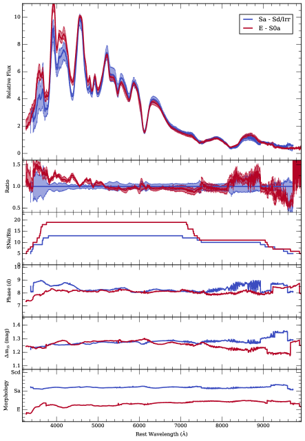
Figure 36: Same format as Figure 14. The blue curves show the properties of our late-type composite spectrum and the red curves show the properties of our early-type composite spectrum. Both of these composite spectra were constructed using a phase bin of $+6<\tau<+11$. The late-type composite spectrum was constructed using a light-curve shape bin of $1.17<$ $\Delta m_{15}(B)$ $<1.48$ mag. The early-type composite spectrum was constructed using a light-curve shape bin of $1.15<$ $\Delta m_{15}(B)$ $<1.45$ mag.

Overall we see very little difference between composite spectra constructed from SNe with differing host galaxy environments. In Figure 34 the late- and early-type composite spectra have effective phases of $-2.4$ and $-2.7$ days and an effective $\Delta m_{15}(B)$ of 1.28 and 1.29 mag respectively. The 1$\sigma$ bootstrapping uncertainty region of the early-type composite spectrum is within the 1$\sigma$ bootstrapping uncertainty region of the late-type composite spectrum at all wavelengths except for the red side of the Ca H&K absorption feature, and at the bluest wavelengths (${<}3500$ Å). This Ca H&K feature is also double troughed in the early-type composite spectrum unlike the late-type composite spectrum. Since the average values of $\Delta m_{15}(B)$ are different by ${\sim}0.1$ mag at the bluest wavelengths, we may be able to attribute the differences in composite spectra at these wavelengths to a difference in average light-curve shape.

Post maximum light the host morphology-controlled composite spectra are also very similar with some consistent differences. The composite spectra in Figure 35 represent the late- and early-type subsamples and have effective phases of $+2.35$ and $+2.52$ days and an effective $\Delta m_{15}(B)$ of 1.30 and 1.29 mag respectively. There is one region near ${\sim}\ 4600$ Å where the late-type composite spectrum has a slightly larger flux. There are also some slight differences in the Calcium absorption features. The early-type composite spectrum has slightly larger flux in the Ca II near-infrared (NIR) triplet absorption region.

Our final set of composite spectra for late and early-type host morphologies have effective phases of $+8.4$ and $+8.1$ days and an effective $\Delta m_{15}(B)$ of 1.28 and 1.25 mag respectively. The 1$\sigma$ bootstrapping uncertainty regions are consistent at all wavelengths except in two regions. We see an excess flux in the early-type composite spectrum near the peak redward of the Si II $\lambda 4130$ feature. Additionally, we see slightly weaker Ca near-infrared triplet absorption in the early-type composite spectrum. We see slightly weaker Ca H&K absorption in the early-type composite spectrum at +3 and +8 days, but these differences are consistent with the 1$\sigma$ bootstrapping uncertainty regions of the late-type composite spectra at those epochs. It is important to note that while the spectra between each of these subsamples are different, some of the same SNe may contribute to the composite spectra at different epochs.

Across multiple epochs there is some evidence for weaker Ca II absorption in the early-type composite spectra. Since this difference is more evident in the Ca II NIR triplet absorption feature, we investigate the evolution of the equivalent width (EW) of this feature from the individual spectra contributing to these composite spectra. These measurements are displayed in Figure 37. Here, measurements coming from the same SNe are connected by lines and the black curve is the best fit linear evolution for the whole sample. We see a very slight tendency for the evolution of the Ca II NIR triplet EW for SNe residing in late-type galaxies (blue points) to lie above the mean evolution, and a very slight tendency for the evolution of the Ca II NIR triplet EW for SNe residing in early-type galaxies (red points) to lie below the mean evolution. To quantify this difference, we measure the mean residual per SN relative to our best fit evolution of the EW of the Ca II NIR triplet. In Figure 38, we show the distribution of these residuals for two bins of host galaxy morphology. The mean Ca II NIR triplet EW residual for late- and early-type host galaxies are $29\pm 2$ Å, and $4\pm 2$ Å respectively. We perform a Kolmogorov-Smirnov test with these data and find a p-value of 0.60, suggesting that we cannot reject the hypothesis that these residual distributions are drawn from the same population. Nonetheless, the tentative evidence for a difference in the strength of the Ca feature is intriguing.

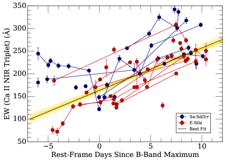
Figure 37: Ca II NIR Triplet EW evolution for SNe residing in late (blue points) and early (red points) type galaxies. Measurements coming from the same SNe are connected by lines. The black curve is our linear best fit to the evolution of the whole sample ($y=(9.4\pm 0.6)x+163\pm 4$)). The yellow curves are best fit lines generated from bootstrap resampling of the data.

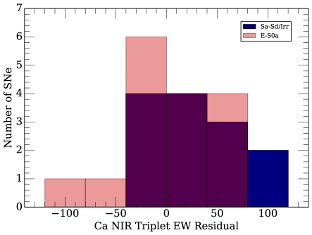
Figure 38: Histograms of the late (blue) and early (red) type mean Ca II NIR Triplet EW residuals per SN from Figure 37.

It is possible that these weaker Ca features can be explained by differences in progenitor metallicity. The simulations presented in De et al. (2014) and Miles et al. (2016) show decreasing ⁴⁰Ca yields with increasing metallicity while ²⁸Si yields stay constant. At each phase, our early-type composite spectra show weaker Ca II features than their late-type analogs and Si II features remain roughly constant (especially near maximum light). However, Miles et al. (2016) also predict that the the strongest effects of metallicity on spectra of SNe Ia should occur in the regions near ${\sim}4200$Å and ${\sim}5200$Å. Our early- and late-type composite spectra tend to be consistent and within the bootstrapping uncertainty regions in these wavelength regions.

The subdivision of our sample by host-galaxy morphology also shows our need for more data in these fine-grained groupings. Since there is a strong correlation between host-galaxy morphology and light-curve shape, disentangling effects of $\Delta m_{15}(B)$ from effects caused by the SN environment is difficult with our limited sample sizes. Although not significant, the differences that we see in Ca II absorption features between our late- and early-type composite spectra is intriguing and could be further investigated with more spectra. This analysis also shows the potential for our composite spectra to uncover minor trends in the spectral features of SNe Ia.

6 Discussion and Conclusions

We have compiled an open-source SQL relational database (kaepora) for observations of SNe Ia. We currently include all spectroscopic data from the largest low-z spectroscopic samples as well as UV data from HST and Swift. This amounts to 4975 spectra of 777 SNe. We have inspected these data for quality and enhanced the data by removing galactic emission lines and cosmic rays, generating variance spectra, and correcting for the reddening caused by both MW and host-galaxy dust. The resulting product is a fully homogenized and accessible sample of SN Ia spectra.

We construct Gini-weighted composite spectra from subsets of these data with sufficient metadata to estimate phase and correct for host-galaxy extinction. We generate 62 independent, phase-binned composite spectra with at least 20 contributing spectra covering phases $-11$ - $+271$ days. We also generate $\Delta m_{15}(B)$-binned composite spectra for a variety of effective light-curve shapes and phases. The maximum-light $\Delta m_{15}(B)$-binned composite spectra range from $\Delta m_{15}(B)$ $=0.86-1.87$ mag. Finally, we investigate the differences between composite spectra generated from SNe Ia residing and late-type and early-type galaxies. Wavelength ranges vary between composite spectra because we require at least 5 SNe to contribute at any given wavelength. Using these composite spectra we are able to reproduce and verify the following trends:

• General evolution of spectral features with phase for normal SNe Ia

• $B-V$ color evolution of normal SNe Ia

• Si II $\lambda 6355$ velocity evolution of normal SNe Ia

• General spectral trends with $\Delta m_{15}(B)$ at maximum light

• Correlation of continuum with $\Delta m_{15}(B)$

• Correlation of $\mathcal{R}$ (Si II) with $\Delta m_{15}(B)$

• Lower Si II $\lambda 6355$ velocities in SNe with extreme values of $\Delta m_{15}(B)$

• Na I D absorption in slower-declining SNe

• Na I D absorption in SNe residing in late-type galaxies

These numerous verifications assure us that the data in our database are of very high quality, which is encouraging for the large number of studies that we include. The additional metadata in our database (see Table 2) will be useful for future studies.

Our phase and $\Delta m_{15}(B)$-binned composite spectra are in good agreement with other template SN Ia spectra. In general the continua of composite spectra for normal SNe Ia are best matched by the Hsiao and Foley template spectra. This was achieved without any generic spectral warping. We have also demonstrated that larger bin sizes in phase and $\Delta m_{15}(B)$ can be used to produce composite spectra that are representative of SNe with the same average properties.

Finally, we examine the subtle spectral differences of composite spectra generated from samples with differing host-galaxy morphologies. Since we can control for both phase and light-curve shape, the remaining significant spectral differences should be related to the progenitor environments of these SNe Ia. Overall the composite spectra representing SNe occurring in late- and early-type environments are very similar at multiple epochs. We see a slight trend for weaker Ca II absorption in composite spectra representing SNe Ia occurring in early-type environments. However, by investigating the Ca NIR triplet EW evolution of these SNe, we do not find significant evidence for the association of these differences with two distinct populations.

Our primary goal for this work is to present kaepora to the community along with the tools that we developed for its validation. We encourage members of the community to use these tools where they see fit. We also strongly encourage the analysis of individual spectra which kaepora makes very easy.

We hope that our database will become a valuable tool for investigating the spectral properties of SNe Ia. We have demonstrated its utility for making template spectra with arbitrary average properties. While we have investigated some parameters here to demonstrate the power of this new database and technique, there are many potential future investigations using other parameters. Also, the large amount of photometric metadata present in the database should be useful for those not solely interested in spectra. Finally, we would like to emphasize that a particular strength this tool provides is fast testing of hypotheses. Since we have homogenized these observations, subsets of spectra with specific properties can be acquired and investigated via a few lines python code.

References

- Amanullah et al. (2015) Amanullah R., et al., 2015, MNRAS, 453, 3300
- Anupama et al. (2005) Anupama G. C., Sahu D. K., Jose J., 2005, A&A, 429, 667
- Arnett (1982) Arnett W. D., 1982, ApJ, 253, 785
- Benetti et al. (2004) Benetti S., et al., 2004, MNRAS, 348, 261
- Benetti et al. (2005) Benetti S., et al., 2005, ApJ, 623, 1011
- Betoule et al. (2014) Betoule M., et al., 2014, VizieR Online Data Catalog, 356
- Blondin et al. (2006) Blondin S., et al., 2006, AJ, 131, 1648
- Blondin et al. (2012a) Blondin S., et al., 2012a, AJ, 143, 126
- Blondin et al. (2012b) Blondin S., et al., 2012b, AJ, 143, 126
- Branch (1987) Branch D., 1987, ApJ, 316, L81
- Cappellaro et al. (2001) Cappellaro E., et al., 2001, ApJ, 549, L215
- Childress et al. (2013) Childress M. J., et al., 2013, ApJ, 770, 29
- Childress et al. (2014) Childress M. J., Filippenko A. V., Ganeshalingam M., Schmidt B. P., 2014, MNRAS, 437, 338
- Chornock et al. (2006) Chornock R., Filippenko A. V., Branch D., Foley R. J., Jha S., Li W., 2006, PASP, 118, 722
- De et al. (2014) De S., et al., 2014, ApJ, 787, 149
- Elias-Rosa et al. (2006) Elias-Rosa N., et al., 2006, MNRAS, 369, 1880
- Elias-Rosa et al. (2008) Elias-Rosa N., et al., 2008, MNRAS, 384, 107
- Fabricant et al. (1998) Fabricant D., Cheimets P., Caldwell N., Geary J., 1998, PASP, 110, 79
- Filippenko et al. (1992a) Filippenko A. V., et al., 1992a, AJ, 104, 1543
- Filippenko et al. (1992b) Filippenko A. V., et al., 1992b, AJ, 104, 1543
- Filippenko et al. (1992c) Filippenko A. V., et al., 1992c, ApJ, 384, L15
- Filippenko et al. (1992d) Filippenko A. V., et al., 1992d, ApJ, 384, L15
- Fitzpatrick (1999) Fitzpatrick E. L., 1999, PASP, 111, 63
- Folatelli et al. (2013a) Folatelli G., et al., 2013a, ApJ, 773, 53
- Folatelli et al. (2013b) Folatelli G., et al., 2013b, ApJ, 773, 53
- Foley & Kasen (2011) Foley R. J., Kasen D., 2011, ApJ, 729, 55
- Foley & Kirshner (2013) Foley R. J., Kirshner R. P., 2013, ApJ, 769, L1
- Foley et al. (2008a) Foley R. J., et al., 2008a, ApJ, 684, 68
- Foley et al. (2008b) Foley R. J., Filippenko A. V., Jha S. W., 2008b, ApJ, 686, 117
- Foley et al. (2009) Foley R. J., et al., 2009, AJ, 138, 376
- Foley et al. (2010) Foley R. J., Narayan G., Challis P. J., Filippenko A. V., Kirshner R. P., Silverman J. M., Steele T. N., 2010, ApJ, 708, 1748
- Foley et al. (2011) Foley R. J., Sanders N. E., Kirshner R. P., 2011, ApJ, 742, 89
- Foley et al. (2012) Foley R. J., et al., 2012, ApJ, 744, 38
- Foley et al. (2013) Foley R. J., et al., 2013, ApJ, 767, 57
- Foley et al. (2016) Foley R. J., et al., 2016, MNRAS, 461, 1308
- Gal-Yam et al. (2003) Gal-Yam A., Maoz D., Guhathakurta P., Filippenko A. V., 2003, AJ, 125, 1087
- Garavini et al. (2007) Garavini G., et al., 2007, A&A, 471, 527
- Gerardy et al. (2004) Gerardy C. L., et al., 2004, in American Astronomical Society Meeting Abstracts #204. p. 777
- Goldhaber et al. (2001) Goldhaber G., et al., 2001, ApJ, 558, 359
- Guillochon et al. (2017a) Guillochon J., Parrent J., Kelley L. Z., Margutti R., 2017a, ApJ, 835, 64
- Guillochon et al. (2017b) Guillochon J., Parrent J., Kelley L. Z., Margutti R., 2017b, ApJ, 835, 64
- Guy et al. (2007) Guy J., et al., 2007, A&A, 466, 11
- Hachinger et al. (2008) Hachinger S., Mazzali P. A., Tanaka M., Hillebrandt W., Benetti S., 2008, MNRAS, 389, 1087
- Hamuy et al. (2000) Hamuy M., Trager S. C., Pinto P. A., Phillips M. M., Schommer R. A., Ivanov V., Suntzeff N. B., 2000, AJ, 120, 1479
- Hatano et al. (2000) Hatano K., Branch D., Lentz E. J., Baron E., Filippenko A. V., Garnavich P. M., 2000, ApJ, 543, L49
- Hicken et al. (2007) Hicken M., Garnavich P. M., Prieto J. L., Blondin S., DePoy D. L., Kirshner R. P., Parrent J., 2007, ApJ, 669, L17
- Hicken et al. (2009) Hicken M., Wood-Vasey W. M., Blondin S., Challis P., Jha S., Kelly P. L., Rest A., Kirshner R. P., 2009, ApJ, 700, 1097
- Howell (2001) Howell D. A., 2001, ApJ, 554, L193
- Howell et al. (2009) Howell D. A., et al., 2009, ApJ, 691, 661
- Hsiao et al. (2007) Hsiao E. Y., Conley A., Howell D. A., Sullivan M., Pritchet C. J., Carlberg R. G., Nugent P. E., Phillips M. M., 2007, ApJ, 663, 1187
- Jha et al. (2006) Jha S., Branch D., Chornock R., Foley R. J., Li W., Swift B. J., Casebeer D., Filippenko A. V., 2006, AJ, 132, 189
- Jha et al. (2007) Jha S., Riess A. G., Kirshner R. P., 2007, ApJ, 659, 122
- Jones et al. (2018) Jones D. O., et al., 2018, ApJ, 857, 51
- Knop et al. (2003) Knop R. A., et al., 2003, ApJ, 598, 102
- Kotak et al. (2005) Kotak R., et al., 2005, A&A, 436, 1021
- Krisciunas et al. (2011) Krisciunas K., et al., 2011, AJ, 142, 74
- Leibundgut et al. (1993) Leibundgut B., et al., 1993, AJ, 105, 301
- Leonard (2007) Leonard D. C., 2007, in Immler S., Weiler K., McCray R., eds, American Institute of Physics Conference Series Vol. 937, Supernova 1987A: 20 Years After: Supernovae and Gamma-Ray Bursters. pp 311–315, doi:10.1063/1.3682922
- Leonard et al. (2005) Leonard D. C., Li W., Filippenko A. V., Foley R. J., Chornock R., 2005, ApJ, 632, 450
- Li et al. (1999) Li W. D., et al., 1999, AJ, 117, 2709
- Li et al. (2001a) Li W., et al., 2001a, PASP, 113, 1178
- Li et al. (2001b) Li W., Filippenko A. V., Treffers R. R., Riess A. G., Hu J., Qiu Y., 2001b, ApJ, 546, 734
- Li et al. (2001c) Li W., Filippenko A. V., Treffers R. R., Riess A. G., Hu J., Qiu Y., 2001c, ApJ, 546, 734
- Li et al. (2003) Li W., et al., 2003, PASP, 115, 453
- Li et al. (2011) Li W., et al., 2011, MNRAS, 412, 1441
- Matheson et al. (2001) Matheson T., Filippenko A. V., Li W., Leonard D. C., Shields J. C., 2001, AJ, 121, 1648
- Mazzali et al. (2005a) Mazzali P. A., Benetti S., Stehle M., Branch D., Deng J., Maeda K., Nomoto K., Hamuy M., 2005a, MNRAS, 357, 200
- Mazzali et al. (2005b) Mazzali P. A., et al., 2005b, ApJ, 623, L37
- Mazzali et al. (2014a) Mazzali P. A., et al., 2014a, MNRAS, 439, 1959
- Mazzali et al. (2014b) Mazzali P. A., et al., 2014b, MNRAS, 439, 1959
- McCully et al. (2014) McCully C., et al., 2014, ApJ, 786, 134
- Miles et al. (2016) Miles B. J., van Rossum D. R., Townsley D. M., Timmes F. X., Jackson A. P., Calder A. C., Brown E. F., 2016, ApJ, 824, 59
- Modjaz et al. (2001) Modjaz M., Li W., Filippenko A. V., King J. Y., Leonard D. C., Matheson T., Treffers R. R., Riess A. G., 2001, PASP, 113, 308
- Nugent et al. (1995) Nugent P., Phillips M., Baron E., Branch D., Hauschildt P., 1995, ApJ, 455, L147
- Nugent et al. (2002) Nugent P., Kim A., Perlmutter S., 2002, PASP, 114, 803
- Nugent et al. (2011) Nugent P. E., et al., 2011, Nature, 480, 344
- Östman et al. (2011) Östman L., et al., 2011, A&A, 526, A28
- Pan et al. (2015) Pan Y.-C., et al., 2015, MNRAS, 452, 4307
- Pan et al. (2018) Pan Y.-C., Foley R. J., Filippenko A. V., Kuin N. P. M., 2018, MNRAS, 479, 517
- Patat et al. (1996a) Patat F., Benetti S., Cappellaro E., Danziger I. J., della Valle M., Mazzali P. A., Turatto M., 1996a, MNRAS, 278, 111
- Patat et al. (1996b) Patat F., Benetti S., Cappellaro E., Danziger I. J., della Valle M., Mazzali P. A., Turatto M., 1996b, MNRAS, 278, 111
- Pereira et al. (2013a) Pereira R., et al., 2013a, A&A, 554, A27
- Pereira et al. (2013b) Pereira R., et al., 2013b, A&A, 554, A27
- Perlmutter et al. (1999) Perlmutter S., et al., 1999, ApJ, 517, 565
- Phillips (1993) Phillips M. M., 1993, ApJ, 413, L105
- Phillips et al. (1992) Phillips M. M., Wells L. A., Suntzeff N. B., Hamuy M., Leibundgut B., Kirshner R. P., Foltz C. B., 1992, AJ, 103, 1632
- Phillips et al. (1999) Phillips M. M., Lira P., Suntzeff N. B., Schommer R. A., Hamuy M., Maza J., 1999, AJ, 118, 1766
- Phillips et al. (2007) Phillips M. M., et al., 2007, PASP, 119, 360
- Pignata et al. (2008) Pignata G., et al., 2008, MNRAS, 388, 971
- Pskovskii (1977) Pskovskii I. P., 1977, Soviet Ast., 21, 675
- Richardson et al. (2001) Richardson D., Thomas R. C., Casebeer D., Blankenship Z., Ratowt S., Baron E., Branch D., 2001, in American Astronomical Society Meeting Abstracts. p. 1428
- Richmond et al. (1995) Richmond M. W., et al., 1995, AJ, 109, 2121
- Riess et al. (1996) Riess A. G., Press W. H., Kirshner R. P., 1996, ApJ, 473, 88
- Riess et al. (1998) Riess A. G., et al., 1998, AJ, 116, 1009
- Riess et al. (1999) Riess A. G., et al., 1999, AJ, 117, 707
- Ruiz-Lapuente et al. (1993) Ruiz-Lapuente P., et al., 1993, Nature, 365, 728
- Ruiz-Lapuente et al. (1997) Ruiz-Lapuente P., Canal R., Isern J., eds, 1997, Thermonuclear supernovae. Proceedings. NATO Advanced Science Institutes (ASI) Series C Vol. 486, doi:10.1007/978-94-011-5710-0.
- Salvo et al. (2001) Salvo M. E., Cappellaro E., Mazzali P. A., Benetti S., Danziger I. J., Patat F., Turatto M., 2001, MNRAS, 321, 254
- Schlafly & Finkbeiner (2011) Schlafly E. F., Finkbeiner D. P., 2011, ApJ, 737, 103
- Scolnic et al. (2018) Scolnic D. M., et al., 2018, ApJ, 859, 101
- Shappee et al. (2013) Shappee B. J., Stanek K. Z., Pogge R. W., Garnavich P. M., 2013, ApJ, 762, L5
- Silverman et al. (2011) Silverman J. M., Ganeshalingam M., Li W., Filippenko A. V., Miller A. A., Poznanski D., 2011, MNRAS, 410, 585
- Silverman et al. (2012a) Silverman J. M., et al., 2012a, MNRAS, 425, 1789
- Silverman et al. (2012b) Silverman J. M., et al., 2012b, MNRAS, 425, 1789
- Silverman et al. (2015) Silverman J. M., Vinkó J., Marion G. H., Wheeler J. C., Barna B., Szalai T., Mulligan B. W., Filippenko A. V., 2015, MNRAS, 451, 1973
- Simon et al. (2007) Simon J. D., et al., 2007, ApJ, 671, L25
- Stanishev et al. (2007) Stanishev V., et al., 2007, A&A, 469, 645
- Stern et al. (2004) Stern D., et al., 2004, ApJ, 612, 690
- Stritzinger et al. (2006) Stritzinger M., Mazzali P. A., Sollerman J., Benetti S., 2006, A&A, 460, 793
- Thomas et al. (2007) Thomas R. C., et al., 2007, ApJ, 654, L53
- Valentini et al. (2003) Valentini G., et al., 2003, ApJ, 595, 779
- Wang et al. (2008) Wang X., et al., 2008, ApJ, 675, 626
- Wang et al. (2009a) Wang X., et al., 2009a, ApJ, 697, 380
- Wang et al. (2009b) Wang X., et al., 2009b, ApJ, 699, L139
- Wells et al. (1994a) Wells L. A., et al., 1994a, AJ, 108, 2233
- Wells et al. (1994b) Wells L. A., et al., 1994b, AJ, 108, 2233
- Yamanaka et al. (2009) Yamanaka M., et al., 2009, PASJ, 61, 713
- Yaron & Gal-Yam (2012) Yaron O., Gal-Yam A., 2012, PASP, 124, 668
- Zhang et al. (2010) Zhang T., et al., 2010, PASP, 122, 1