2cm2cm1.5cm1.5cm
Orthodiagonal anti-involutive Kokotsakis polyhedra
Abstract.
We study the properties of Kokotsakis polyhedra of orthodiagonal anti-involutive type. Stachel conjectured that a certain resultant connected to a polynomial system describing flexion of a Kokotsakis polyhedron must be reducible. Izmestiev [3] showed that a polyhedron of the orthodiagonal anti-involutive type is the only possible candidate to disprove Stachel’s conjecture. We show that the corresponding resultant is reducible, thereby confirming the conjecture. We do it in two ways: by factorization of the corresponding resultant and providing a simple geometric proof. We describe the space of parameters for which such a polyhedron exists and show that this space is non-empty. We show that a Kokotsakis polyhedron of orthodiagonal anti-involutive type is flexible and give explicit parameterizations in elementary functions and in elliptic functions of its flexion.
1. Introduction
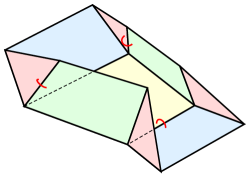
A Kokotsakis polyhedron is a polyhedral surface in which consists of one -gon (the base), quadrilaterals attached to every side of the -gon, and triangles placed between each pair of two consecutive quadrilaterals. Such surfaces are rigid in general. However, there exist special classes of flexible surfaces, that is, ones that allow isometric deformations. Flexible Kokotsakis polyhedra were studied by several authors: in the PhD thesis of Antonios Kokotsakis and in [4]; Nawratil [5] studied flexible Kokotsakis polyhedra with triangular base; and in [8] some classes of flexible Kokotsakis polyhedra with quadrilateral base were found. The question of complete classification for the case was open. Using Bricard’s approach [1], Stachel and Nawratil [6, 7, 9] with the use of the following trigonometric substitution
| (1) |
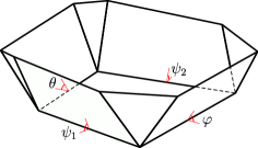
expressed the dependencies between the dihedral angles , , , (see Figure 1) as a polynomial system in , , , :
| (2) | ||||||
They studied this system with respect to different factorizations of the resultant of and as polynomials in , and they classified all classes of flexible Kokotsakis polyhedra with quadrilateral base for reducible . Stachel conjectured that there is no flexible Kokotsakis polyhedron whose system has the irreducible resultant.
Considering a complexified version of system (2), Izmestiev [3] classified all possible classes of flexible polyhedra disregarding reality and embeddability. In particular, from the results of [3] it follows that there is only one possible candidate for a flexible Kokotsakis polyhedron with the irreducible resultant . He called elements of this class Kokotsakis polyhedra of orthodiagonal anti-involutive type (OAI).
In this paper we study the properties of OAI Kokotsakis polyhedra. We find an explicit parameterization in elementary functions of all solutions of the system (2) for this type and show that there are solutions which may be embedded in the real three-dimensional space. We prove that the resultant is always reducible, which confirms Stachel’s conjecture. In addition, we provide a simple geometric proof of this fact in Theorem 6 that directly follows from the results of [3].
The rest of the article is organized as follows. We give the definition of an OAI Kokotsakis polyhedron in Section 2 together with algebraic formulas for coefficients of the polynomial systems required for further analysis. However, we postpone an explanation of their geometric meaning to Section 6. Section 3 is devoted to the description of all solutions of the system (2) for an OAI Kokotsakis polyhedron, which is the system (10). In Theorem 2 of this Section, we give an explicit parameterization in elementary functions of all branches of the solution. In other words, here we come up with a description of all possible flexions of an OAI polyhedron when all planar angles are given. In Section 4 we study a four parameter system that describes planar angles of all flexible OAI Kokotsakis polyhedra. We give a full parameterization of the solution set of this system in terms of the angles of the base quadrilateral and one additional parameter in Theorem 4. Summarizing the results, we introduce in Section 5 an algorithm for constructing a flexible OAI Kokotsakis polyderon for a given base quadrilateral without right angles. In addition, we present results from the numerical screening of the space of parameters. In Section 6, we discuss the geometry behind the definitions and equations that we use, show that there is a nice flattening effect in the case of the orthodiagonal anti-involutive surface, and give a simple proof of Stachel’s conjecture using it. In Appendix 8 we prove some technical results.
Remark 1.1.
We formulate all the theorems in such a manner that the reader can understand them right after reading the definitions of Section 2. This allows to use formulas from these theorems and construct a flexible polyhedron without going into the details of the proofs.
2. Definitions
In this section we give an algebraic description of a Kokotsakis polyhedron of the orthodiagonal anti-involutive type. We do not discuss the nature of the written equations here. A comprehensive explanations can be found in [3]. However, we give a brief explanation in Section 6, where we show that Stachel’s conjecture is a simple consequence of the results from [3].
Vertices of a Kokotsakis polyhedron and the values of its planar angles at the interior vertices are denoted as in Figure 2. Clearly, it is only a neighborhood of the base face that matters: replacing, say, the vertex by any other point on the half-line does not affect the flexibility or rigidity of the polyhedron.
For each of the four interior vertices , , , consider the intersection of the cone of adjacent faces with a unit sphere centered at the vertex. This yields four spherical quadrilaterals with side lengths in this cyclic order. Let , , , and be the exterior dihedral angles at edges and respectively. Clearly, it suffices to parameterize these dihedral angles in order to describe a flexion of a Kokotsakis polyhedron.
2.1. Orthodiagonal quadrilaterals
We call a spherical quadrilateral orthodiagonal if its diagonals are orthogonal. A spherical quadrilateral is called elliptic if its planar angles satisfy
Let be a spherical elliptic orthodiagonal quadrilateral with side lengths and angles denoted as in Figure 3. Then the orthodiagonality of is equivalent to the following identity:
| (3) |
(see Lemma 8.1 below).
By definition put . Then satisfy the following equation (see Lemma 4.13 in [3]):
| (4) |
where are the so-called involution factors defined as follows
| (5) | |||
| (6) |
and is given by
| (7) |
The involution factors and are well-defined real numbers different from .
2.2. Orthodiagonal anti-involutive type
A Kokotsakis polyhedron belongs to the orthodiagonal anti-involutive type, if its planar angles satisfy the following conditions.
-
1)
All quadrilaterals are orthodiagonal and elliptic:
-
2)
The involution factors at common vertices are opposite:
(8) -
3)
The involution factors and satisfy the following system:
(9)
By (4) and (8), variables of a Kokotsakis polyhedron of the orthodiagonal anti-involutive type satisfy the system
| (10) | |||
We are interested only in the non-trivial solutions of this system, that is, the one-parametric branches of the solution set chosen in a way that each of is not a constant.
Remark 2.1.
System (9) expresses the proportionality of the resultants and .
2.3. Five-parametric system
The problem of description of all flexible Kokotsakis polyhedra of the orthodiagonal anti-involutive type is separated into two sub-problems in a natural way:
-
•
to describe the planar angles such that the corresponding polyhedron is of the orthodiagonal anti-involutive type;
-
•
to describe its flexion, i.e. the trajectory in dihedral angles space.
The latter is equivalent to solving system (10), which describes the configuration space of , with given coefficients , , that satisfy (8) and (9). In Theorem 2 we give a complete parameterization with one variable of a solution set of this system.
It is more complicated to describe all admissible planar angles . It is natural to consider the angles as parameters. Since , it is a three parametric family. From the algebraic point of view, system (9) together with identities (8) and definition (7) is a system of three equations in four variables . It is enough to introduce one more parameter to describe a solution, which we do in Section 4. On the other hand, given and together with (8) one can recover angles from
| (11) |
in the case and compute from
| (12) |
if the right-hand side is in . That is, the angles of the base quadrilateral and determine all the needed data to construct a Kokotsakis polyhedron.
It is not obvious that such a geometric construction exists even one finds all the planar angles of an OAI Kokotsakis polyhedron. However, the following result gives the answer to this question.
Definition 2.3.
We consider the following geometric assumptions on and
-
1.
are the angles of a quadrilateral without right angles, that is and , where and
- 2.
- 3.
-
4.
Spherical quadrilaterals with sides , where , are elliptic.
Theorem 1.
Let and meet the geometric assumptions of Definition 2.3. Then a Kokotsakis polyhedron with spherical quadrilaterals with sides exists, it is flexible and all its possible flexion are parameterized as in Theorem 2.
Remark 2.4.
We find it interesting that if and meet only first two of the geometric assumptions, a non-trivial solution of (10) still exists and is given by Theorem 2. However, the angles might fail to be determined by (12) if the absolute value of the right-hand side of (12) is bigger than 1. This follows from Lemma 4.1 and a condition of the existence of non-trivial solution in Theorem 2.
3. The real part of the configuration space
The form of solution in real numbers of the system (10) depends on the signs of . That is, it depends on the signs of the entries in the matrix
We call arrangement of signs in this matrix a sign pattern. It will be shown below in Lemma 3.1 that there is a unique possible arrangement of signs up to re-enumeration of the vertices. Using this observation, we assume that
| (13) |
Theorem 2.
According to assumption (13) and by condition , we see that all values under square roots in the previous formulas are positive.
3.1. Uniqueness of the sign pattern
Due to system (9), we have some restrictions to possible signs of .
Lemma 3.1.
Proof.
We first show that for some vertex both . By the third equation in (9), we see that either or . If in this positive product both factors are also positive, we have found the sought vertex. If however both coefficients are negative, from the fact that in a sign pattern there are always exactly four pluses and four minuses (follows from (8)), we conclude that if in sign pattern there is a row of minuses, there should be a row of pluses.
As cyclic permutations just change the order of vertices of the base quadrilateral, we assume that and . In other words, known signs are:
We rewrite equation of (10) in the following way:
Since absolute values of both parentheses are greater or equal to 2, for this equation to have a one-parametric solution (and not discrete set of points), we obtain
By the third equation in (9)
Hence, or, equivalently, . By the first equation in (9), we get that . Finally, the only possible sign pattern is (15). ∎
3.2. Reduced system
To simplify equations of system (10) and (9), we scale the variables and consider a reduced system (after the re-enumeration of vertices so that and ). Making the following substitution in system (10):
| (16) | ||||||
we get 4 equations:
| (17) |
where and are positive.
System (9), which describes conditions for the proportionality of the resultants, can be rewritten in the form
| (18) |
3.3. Equation with positive signature
One can see that and are of the same sign, and there is a symmetry of the solution . We assume that . Now we consider new coordinates In these coordinates, the equation takes the form:
| (20) |
Thus, there is a one-parametric real solution set if and only if
| (21) |
which we have already shown in Lemma 3.1.
Solution to Equation (20) can be parameterized in an explicit way. Let , . Then we can parameterize solution of (20) as
where , which, by direct calculations, leads to the following representation of and :
where
Moreover, the solution of (20) is bounded in the plane . This means that and cannot be equal or . Or, speaking geometrically, if equation (19) describes the configuration space of the spherical quadrilateral of a Kokotsakis polyhedron, then the corresponding side quadrilaterals never cross the base plane (see Lemma 6.5).
3.4. Proof of Theorem 2
Proof.
By the results of Subsection 3.3 and by (21) in particularly, we see that the real solution of the system is nonempty and non-trivial if and only if (recall that and are positive). Also in Subsection 3.3, the equation with positive sign signature was resolved, which leads to the explicit formulas for and . One can prove that the formulas for and from (14) are the solution of the system by the direct substitution. However, we want to show that we have found all branches of the solution. We can consider system (17) and variables instead of . One can see that the solution of the first equation is given in Subsection 3.3, the second equation is quadratic in , the fourth equation is quadratic in . Hence, we have two possible branches of solution for both and , and there are at most four branches of the solution up to the symmetry . So the only difficulty is to check that we have chosen the correct branches to meet the third equation of the system. We claim that the latter obstacle implies that there are exactly two branches of the solution with positive and . Hence, we described all possible solution with positive and . Indeed, fixing , we fix . Therefore, fixing , we fix . But changes its value if we change the branch for . Therefore, there is a unique branch of for each branch of . By the symmetry , we describe all branches of the solution. ∎
3.5. Reducible resultant
As a linear substitution does not change the property of irreducabillity of the resultant, we consider the resultant of the first two equations of reduced system (17) as polynomials in is given by:
When from (18) holds true, the resultant is the product of the following polynomials:
This can be checked by a direct calculation. Moreover, as we show in Lemma 6.6 below, the resultant is reducible if and only if
3.6. Symmetries
Here we discuss some symmetries hidden in our equations.
First of all, the symmetry or, equivalently, in terms of the dihedral angles is just the symmetry with respect to a plane of the base quadrilateral. Clearly, it does not change a configuration.
Secondly, our equations allow us to make the following substitution for planar angles at vertex of the base quadrilateral:
-
(1)
-
(2)
-
(3)
Clearly, the corresponding spherical quadrilateral remains elliptic, and the involution factors do not change. These symmetries may help with avoiding self-intersections of a polyhedron.
3.7. Elliptic parameterization
In [3] the author parameterized a solution of (4) in terms of the Jacobi elliptic sines. Using the results of that paper, we provide a sketch of the proof of the following result in which we give an elliptic parameterization of the solution set of system (10). A comprehensive description of the OAI flexible Kokotsakis polyhedra with the use of elliptic functions can be found in [2].
Theorem 3.
Let satisfy systems (9), (8) and assumption (13). Then system (10) has a real non-trivial one-parametric set of solutions if and only if . The solution set has four branches, which, up to the symmetry , are given by
| (22) |
where is the elliptic modulus given by and are the quarter periods of elliptic sine with modulus ; is a parameter and the choice of and in and is simultaneous.
Sketch of the proof..
It was shown in [3] that the solution set of (4) has a parameterization of the form
where is a quarter-period of that is, and the amplitudes belong to Moreover, there is a table with explicit formulas for as functions of in Lemma 4.17 of [3]:
From this table, we see that the elliptic modulus is a function of Since and by the choice of sign pattern (15), we get that the elliptic moduli of all four spherical quadrilaterals are the same in case of an OAI polyhedron. Then it is easy to recover what a quarter-period shift one can use in each equation of (17). ∎
Remark 3.1.
It follows that the OAI type of Kokotsakis polyhedra is a special class of the elliptic equimodular type in the notation of [3].
We note that the parameterizations from Theorem 3 cannot be transformed to the parameterizations given by Theorem 2 using linear substitution of the parameter as the first one uses elliptic functions that are not elementary. However, under the substitution the parameterization given by Theorem 3 is quite close to the parameterization given by Theorem 2 for small enough (see Figure 13 and Figure 14).
4. Planar angles of a flexible polyhedron
In this section, we study and that meet the first two of the geometric assumptions. In the following theorem we manage to parameterize all such . In fact, for solving system (9), we need to make it more symmetrical with a proper substitution, and we use new variables for this purpose. We introduce these substitutions in the theorem and explain their sense later.
Theorem 4.
Let all and meet the first two of the geometric assumptions. Put
| (23) |
Then there exists and a proper choice of signs such that
| (24) |
where are functions of with the symmetries
| (25) |
and is given by
| (26) |
where
with
It is very intriguing that for each value of in this theorem such that all values under square roots are positive, system (10) has real non-trivial solutions.
Lemma 4.1.
4.1. A new symmetric system
System (9) can be rewritten in the following form:
| (27) |
Make a substitution
| (28) |
and let
| (29) |
Then system (27) is equivalent to the system of the following three equations , and . Adding a linear dependent equation, system (27) can be rewritten in the following equivalent way
| (30) |
where is parameter.
System (8) takes the form:
| (31) |
The equations of system (30) are linear in both or . Since, by the definitions, , are real and , we obtain a restriction on the values of , :
| (32) |
4.2. Proof of Theorem 4
Proof.
Restriction (32) yields positivity of radical expressions in (24). So, it suffices to prove identities (25) and (26). We start with the latter one.
Using exclusion technique to find from system (30) is equivalent to finding roots of an equation of the second degree with coefficients determined by the coefficients of the system (30). Indeed, from the equation , we see that functions or are linear fractional transformations. Since composition of two linear fractional transformations is a linear fractional transformation, finding , and , , we obtain two different Möbius transformation functions for Therefore, general solution has a form:
| (33) |
where and are polynomials of 2nd degree and is a polynomial of 4th degree. However, we noticed that always have a full square as a multiplier, when . Using our substitution (23), we managed to factorize , merge two branches in (33) and obtain (26). The explicit formulas for the coefficients were found and can be verified with the use of a system of computer algebra. We used Wolfram Mathematica 11 for this purpose.
Since equation (33) is obtained by the exclusion technique, it describes all possible . Note that it has two branches, however we have only one in (26). So we need explain how we managed to merge the branches. The radical expression in (33) equals to . Since is the only function that have linear terms in and , substitution changes the sign of and preserves the values of , , in (26), that is, it merges two branches of (33).
Let us explain identities (25). There are no more solutions as each equation of (30) is linear in either or . Apart from checking (25) with direct calculations, we provide the following arguments. The dependencies on , , arise from re-enumeration of vertices, Explanation of a “phase shift” of is trickier. By the symmetry of the system (30), it is enough to explain a “phase shift” for . Fixing , we have exactly one possible value for by the equation and two possible branches in (33) rewritten for . The “phase shift” corresponds to the right choice of the branch. ∎
4.3. Proof of Lemma 4.1 and Theorem 1
Proof of Lemma 4.1.
By the first equation in (27), either , or , are both non-zero and have the same sign. Again, by Pigeonhole principle, it implies that there is a pair with positive numbers. Without loss of generality, let it be pair , . By the second equation, the latter implies that , has the same sign. We claim that they are negative, and, therefore, we have the case of the right sign pattern.
Theorem 1 is a direct consequence of this lemma.
5. Algorithm
In the following Theorem, we summarize all needed steps to construct a flexible Kokotsakis polyhedron of the orthodiagonal anti-involutive type and to describe its flexion using given values of the angles of the base quadrilateral. We are always looking for angles in interval However, one can allow to the angles and to be in
Theorem 5.
Given parameters , the algorithm of constructing a flexible Kokotsakis polyhedron of the orthodiagonal anti-involutive type is the following:
-
(1)
Check whether meet the first of the geometric assumptions, that is, they form a quadrilateral without right angles.
-
(2)
Calculate using substitution (23).
-
(3)
Check whether there exists such that , , , given by (26) and (25) satisfy inequality (32) (see Subsection 5.1 for how this can be done). Set , , , .
-
(4)
Calculate the angles and from
where are chosen in a way to satisfy: . Select angles to be from to .
-
(5)
Check that . Find using (12).
-
(6)
Check that obtained spherical quadrilaterals with sides are elliptic.
- (7)
-
(8)
Re-enumerate vertices to get (15) as a sign pattern of the system.
-
(9)
Find using formulas of Theorem 2. Calculate dihedral angles using
Proof.
Remark 5.1.
We do not check whether the obtained surface is not self-intersecting. There remains a possibility that at every moment during flexion, there are two intersecting facets.
It’s possible to derive a implicit formula for a set of (or, equivalently, ) for which there exists such that and the angles are well-defined. However, the resulting formula is likely to be enormous and incomprehensive. We instead explain how to check the conditions and show the result of numerical screening in the next subsection.
5.1. Screening of the space of parameters
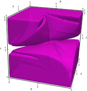
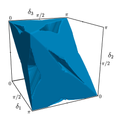
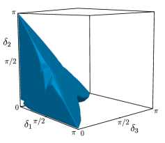
In Theorem 5, one need to find a proper parameter for a given angles (or, equivalently, ). We run a computer screening and found numerically the set of for which there exists such that are given by Theorem 4 and meet the geometric assumptions. The result of our numerical computation is in Figure 4, here we do not show surfaces on which at least one is not elliptic. Figure 5 shows the result of screening in coordinates for convex and non-convex base quadrialareals.
We claim that it can be done with an arbitrary precision or, probably, explicit formulas for the boundary can be found, as all the restrictions on are polynomial.
More precisely,
-
(1)
is clearly a polynomial in .
-
(2)
(and others comparisons for with constant ) is equivalent to a proper system of the following polynomial inequalities
and comparison of , and with zero.
-
(3)
is well-defined if and only if
By the latter is
which is equivalent to a system of polynomial inequalities.
6. Geometric properties
6.1. The configuration space of a spherical quadrilateral
Side lengths and angles of a spherical quadrilateral are denoted in Figure 6, and .
As was discovered by Bricard [1], the equation of the configuration space of has the form
| (34) |
where the coefficients are trigonometric functions of the angles of
By allowing to take complex values, we arrive at a complex algebraic curve
| (35) |
with two coordinate projections
| (36) |
If is of elliptic type then is an elliptic curve. The projections in (36) are two-fold branched covers with exactly 4 points in the branch set. Since equation (34) is quadratic in one variable, one can easily find explicit formulas for points of the branch set by solving a quadratic equation. The complete classification of different classes of spherical quadrilaterals and their branch sets can be found in [3] Subsection 2.4 and Lemma 4.10.
Denote by
the deck transformations of and . If and are real, we can give a geometric interpretation of these involutions: and act by folding the quadrilateral along one of its diagonals, see Figure 7. This means that realizable branch points correspond to a degenerate case when quadrilateral becomes a triangle. Hence, we conclude
Lemma 6.1.
Let be a spherical quadrilateral of elliptic type. We use the notation as in Figure 6 and put Then belongs to the branch set of if and only if
6.2. Scissors-like linkage
Two adjacent vertices of the base quadrilateral share the common dihedral angles, which means the corresponding spherical quadrilaterals are coupled by means of the angle (see Figure 8).
There are four such scissors-like linkages corresponding to edges , , and of the base quadrilateral in a Kokotsakis polyhedron. Isometric deformations of the polyhedron correspond to motions of these linkages. Algebraically speaking, these linkages are described by the rows and columns of system (2), and the system itself describes possible dihedral angles of the polyhedron. Moreover, a Kokotsakis polyhedron is flexible if and only if the system of polynomial equations (2) has a one-parameter family of solutions over the reals ([3], Lemma 2.2). One possible approach to find a solution is as follows:
-
(1)
consider a pair of opposite edges and together with corresponding linkages, which are described by systems and respectively;
-
(2)
exclude common variables and in the corresponding systems by computing the resultants and .
The polyhedron is flexible if and only if the algebraic sets and have a common irreducible component. This means that they are reducible or irreducible simultaneously. Stachel and Nawratil described all flexible classes for reducible and .
Remark 6.1.
Geometrically speaking, the zero set of the resultant gives an implicit dependence of the non-common angles of spherical quadrilaterals and , and does the same for and . The polyhedron is flexible if and only if these “dependencies” have a common branch, that is, on can join the scissors-like linkages and during the corresponding flexion.
Izmestiev [3] considers the complexified configuration space of a spherical linkage (that is, the set of all complex solutions of the corresponding polynomial system). The following lemma is a direct consequence of the results of [3]. It follows from Lemma 5.1 and assertion (4) of Lemma 4.10 of that paper.
Lemma 6.2.
Let polynomial system describe a scissors-like linkage of two elliptic spherical quadrilaterals and The resultant is reducible if and only if the branch sets of and coincide.
Remark 6.2.
We note that Izmestiev understands the property of irreducibility of a coupling of two spherical quadrilaterals as the irreducibility of an algebraic set that describes the corresponding complexified configuration spaces. One should not confuse the properties of irreducibility of the resultant with the irreducibility of the coupling.
As was mentioned above, Izmestiev showed that there is only one possible candidate for a flexible Kokotsakis polyhedron with irreducible resultant . In particular, all scissors-like linkages of such a polyhedron must be of a special type, which the author called anti-involutive coupling.
6.3. Anti-involutive coupling and its properties
A coupling of two orthodiagonal quadrilaterals is called anti-involutive if their involution factors at the common vertex are opposite, e.g. for two coupled spherical quadrilaterals associated with the edge .
Lemma 6.3.
Let spherical orthodiagonal quadrilaterals and form a scissor-like linkage as in Figure 9 with the involution factors and in the common vertex. Then
Proof.
Equation (4) implies that the involutions of an orthodiagonal quadrilateral are given by
Therefore, the condition is equivalent to compatibility of the involutions of the coupled quadrilaterals at their common vertex:
On the other hand, the involution changes the angle of the first quadrilateral at the common vertex from to , and the angle of the second quadrilateral from to . The compatibility means that the angles at the common vertex remain equal after the involution: . Because , this is equivalent to , .
Observe that exchanging and changes the sign of the involution factor. Thus, if we rotate the left half of the scissors linkage, then the condition transforms to . On the other hand, this exchanges the angles and . This proves the second part of the lemma. ∎
Lemma 6.4.
In an antiinvolutive () linkage of two orthodiagonal quadrilaterals, if one of the angles and in Figure 10 becomes or , then the other one does as well.
Proof.
Indeed, if and only if ∎
6.4. Geometric properties of orthodiagonal anti-involutive type polyhedra
From the definition of an OAI polyhedron, we see that all four linkages of it are anti-involutive. Applying Lemma 6.4, we observe the following flattening effect.
Corollary 6.1.
In a flexible OAI Kokotsakis polyhedron the dihedral angles at the three bold edges in Figure 11 vanish or become at the same time.

Using Theorem 2, it is quite easy to understand what kind of flattening has a flexible OAI Kokotsakis polyhedron.
Lemma 6.5.
Two dihedral angles of a flexible OAI Kokotsakis polyhedron never become or , the two other dihedral angles become and on each brunch of the solution given by Theorem 2
Proof.
We use the notation of Section 3. If one of the angles , , , is or then the corresponding variable is or Since substitution (16) just scales the variables, the same happens to the corresponding variable of system (17). Let us consider it for simplicity. By Subsection 3.3, the variables of the first equation of (17) (with positive signature) never become or Also, each branch of the solution of the whole system contains all solutions of the first equation up to the symmetry Moreover, since then at two different points of the solution of the first equation. Therefore, by the second equation, becomes or at these points on each branch of the solution of the whole system. It is easy to see that is different at this points. So it must be and at these points, and it can have these values only at these points. A similar argument works for and ∎
Summarizing all results, we prove Stachel’s conjecture.
Theorem 6.
Stachel’s conjecture is true. The resultant of a real flexible OAI Kokotsakis polyhedron is reducible.
Proof.
We use the notation of the first three sections. By Lemma 6.2, it is enough to show that the branch sets for and coincide. By Lemma 6.1, it suffices to prove that the dihedral angles at edges and (see Figure 2) become 0 or simultaneously at four different points. This follows from Corollary 6.1 and Lemma 6.5. ∎
Remark 6.3.
Lemma 6.6.
The resultant of the first two equations of system (17) is reducible if and only if
Proof.
It is easy to see that belongs to the branch set of if and only if
From here, the branch set is
Similar, the branch set of for the second equation is
These sets coincide exactly when ∎
7. Example
In this section we consider the construction of a flexible OAI Kokotsakis polyhedron with angles of the base quadrilateral:
We selected . Following the procedure in Theorem 5, we get
In Figure 12 we show the state of the given polyhedron when we observe the flattening effect.
In this case, we have And we observe the effect of a closeness of parameterization mentioned in Section 3. Hardly one can observe the difference between two parameterizations.
However, they are different. And we can calculate numerically the difference
8. Appendix: properties of orthodiagonal quadrilaterals
Lemma 8.1.
The diagonals of a spherical quadrilateral with side lenths , , , (in this cyclic order) are orthogonal if and only if its side lengths satisfy the relation
Proof.
Take the intersection point of two diagonals of the quadrilateral. (A pair of opposite vertices determines a big circle. We take one of the two intersection points of these two big circles.) Denote the lengths of the segments between the vertices and the intersection point of the diagonals as shown in Figure 15. By the spherical Pythagorean theorem we have It follows that
∎
Lemma 8.2.
Let satisfy Then there exists a spherical orthodiagonal quadrilateral with side lengths
Proof.
Assume that is the minimum of the sum of two consecutive angles in . If and the construction is obvious. Otherwise, assume that Put sides and with lengths and respectively on the same great circle. Then there is a vertex such that is a right angle and the length of is By the identity, the length of is ∎
References
- [1] R. Bricard. Mémoire sur la théorie de l’octaèdre articulé. Journal de Mathématiques pures et appliquées, 3:113–148, 1897.
- [2] I. Izmestiev. Flexible Kokotsakis polyhedra based on orthodiagonal spherical quadrilaterals. In preparation.
- [3] I. Izmestiev. Classification of flexible Kokotsakis polyhedra with quadrangular base. International Mathematics Research Notices, 2017(3):715–808, 2016.
- [4] A. Kokotsakis. Über bewegliche polyeder. Mathematische Annalen, 107(1):627–647, 1933.
- [5] G. Nawratil. Flexible octahedra in the projective extension of the Euclidean 3-space. J. Geom. Graph., 14(2):147–169, 2010.
- [6] G. Nawratil. Reducible compositions of spherical four-bar linkages with a spherical coupler component. Mechanism and Machine Theory, 46:725–742, 2011.
- [7] G. Nawratil. Reducible compositions of spherical four-bar linkages without a spherical coupler component. Mechanism and Machine Theory, 49:87–103, 2012.
- [8] R. Sauer and H. Graf. Über Flächenverbiegung in Analogie zur Verknickung offener Facettenflache. Mathematische Annalen, 105(1):499–535, 1931.
- [9] H. Stachel. A kinematic approach to Kokotsakis meshes. Comput. Aided Geom. Design, 27(6):428–437, 2010.