Strategies of motion under the black hole horizon

Abstract

In this methodological paper we consider two problems an astronaut faces with under the black hole horizon in the Schwarzschild metric. 1) How to maximize the survival proper time. 2) How to make a visible part of the outer Universe as large as possible before hitting the singularity. Our consideration essentially uses the concept of peculiar velocities based on the ”river model”. Let an astronaut cross the horizon from the outside. We reproduce from the first principles the known result that point 1) requires that an astronaut turn off the engine near the horizon and follow the path with the momentum equal to zero. We also show that point 2) requires maximizing the peculiar velocity of the observer. Both goals 1) and 2) require, in general, different strategies inconsistent with each other that coincide at the horizon only. The concept of peculiar velocities introduced in a direct analogy with cosmology, and its application for the problems studied in the present paper can be used in advanced general relativity courses.

I Introduction

”Elementary” metrics of black holes such as the Schwarzschild or Reissner-Nordström ones are studied very thoroughly and described in many textbooks. Nonetheless, time to time new and, sometimes, quite unexpected aspects of them appear again and again. The aim of the present article is to draw attention to the special class of trajectories situated inside the event horizon of a nonextremal black hole. These trajectories correspond to $\varepsilon=0$ where the integral of motion $\varepsilon$ has inside a horizon the meaning of momentum, not energy. And, among them the most interesting is their subclass when the trajectory strongly bends to the horizon. The results are valid for a quite generic metric but, for definiteness, we concentrate mainly on the Schwarzschild one. There is a number of different issues in this context which, however, turned out to be interrelated due to this class of trajectories. In our previous work zero , we considered high-energy collisions of a particle that follows such a trajectory with ambient ones. Meanwhile, there are also other interesting properties of the same class of trajectories discussed in the present work. Namely, we consider the following questions: (i) the maximization of time before reaching the singularity, (ii) possibility for an observer to see during a finite proper time all future of Universe (this issue was discussed in kras , gpu but account of the trajectories under discussion adds new options not noticed there). Both questions usually attract great attention of a student audience while General Relativity studying. The concept of ”river of space” itself, being a counterpart of the famous concept of ”expanding space” in cosmology, as well as the definition of peculiar velocities introduced in a direct analogy of the corresponding definition in cosmology can be used in advanced General Relativity courses. They show in particular that some intuitively clear concepts in GR represent not the physical situation itself, but mostly the properties of a coordinate system used to describe this picture. Using appropriate coordinate system better suited for a physical problem considered is a necessary skill for scientific work in GR. We hope that the present paper where we study the spherically symmetric static metric in three different frames (one stationary and two different synchronous frames) depending on a particular question considered, would help in achieving this goal.

Throughout the paper, we use geometric units in which fundamental constants $G=c=1$.

II Basic equations

We consider the metric

$$ds^{2}=-fdt^{2}+\frac{dr^{2}}{f}+r^{2}d\omega^{2}\text{,}$$ (1)

where $d\omega^{2}=(d\theta^{2}+\sin^{2}\theta d\phi^{2}).$

We suppose that the metric has the event horizon at $r=r_{+}$, so $f(r_{+})=0$. For the Schwarzschild metric, $f=1-\frac{r_{+}}{r}$, where $r_{+}=2M$ is the horizon radius, $M$ being the black hole mass. The most part of results applies also to generic $f(r)$ with one root. Near the event horizon,

$$f\approx\kappa(r-r_{+})\text{,}$$ (2)

where $\kappa=\frac{f^{\prime}(r_{+})}{2}$ is the surface gravity. In the Schwarzschild case $\kappa=\frac{1}{2r_{+}}$.

We are mainly concerned with the interior of a black hole. Then, it is instructive to make substitutions (see nov61 and fn , page 25)

$$r=-T,t=y,f=-\tilde{f},\text{ }\tilde{f}\geq 0,$$ (3)

where $-r_{+}\leq T\leq 0$. The coordinate $y$ plays the role of a radial coordinate inside the horizon while $T$ has the meaning of time.

Then,

$$ds^{2}=-\frac{dT^{2}}{\tilde{f}}+\tilde{f}dy^{2}+T^{2}d\omega^{2}\text{.}$$ (4)

For the Schwarzschild metric $\tilde{f}=\frac{r_{+}}{r}-1=-1-\frac{r_{+}}{T},$ where $-r_{+}<T\leq 0$.

The metric under discussion looks differently in different regions of space-time. This is a particular manifestation of the fact that in spherically symmetric space-times there exist so-called $R$ and $T$ regions. Namely, let us denote $\rho^{2}$ the coefficient at the angular part. Then, if the vector normal to the surface $\rho=const$ is space-like, the region is called the $R$ one. If such a normal vector is time-like, it corresponds to the $T$ region. Such a classification was suggested in rt . The full space-time diagram of the Schwarazschild eternal black hole includes two $R$ regions $R1$ and $R2$ and two $T$ regions - expanding and contracting ones. This description can be found in many textbooks and monographs. See, e.g. fn . Region $R1$ corresponds to our world while $R2$ represents the ”mirror world”. The second $T$ region and $R2$ region exist only in a mathematical picture which includes black and white eternal hole, and they are absent in a realistic black hole space-times obtained as a result of gravitational collapse.

In the metric (1), (4) there is an integral of motion

$$\varepsilon=-u_{\mu}\xi^{\mu}\text{,}$$ (5)

where $\xi^{\mu}$ is the corresponding Killing vector responsible for translations along the $y$ axis, $u^{\mu}=\frac{dx^{\mu}}{d\tau}$ being the four-velocity, $\tau$ the proper time. Under the horizon, $\varepsilon$ has the meaning of the radial momentum,

$$\varepsilon=-u_{y}.$$ (6)

Three equations of motion within the plane $\theta=\frac{\pi}{2}$ for a geodesic particle read

$$\dot{T}=Z\text{,}$$ (7)

$$\dot{y}=-\frac{\varepsilon}{\tilde{f}}\text{,}$$ (8)

$$m\dot{\phi}=\frac{L}{T^{2}}\text{,}$$ (9)

dot denotes differentiation with respect to the proper time $\tau$. Eq. (8) follows immediately from (6) in the metric (4). If the Killing vector corresponds to rotations, in coordinates $(T,y,\phi)$ it has the form ($0,0,1$), so similar to (6) we have $L=mu_{\phi}$. In this manner, we get eq. (9). Then, from the normalization condition and $\dot{T}>0$ we obtain (7).

Here, $\varepsilon$ can have any sign, $\varepsilon=\pm\left|\varepsilon\right|.$ The case $\varepsilon=0$ is also possible. From the normalization  condition $u_{\mu}u^{\mu}=-1$ and taking into account the forward-in-time condition $\dot{T}>0$, we obtain in coordinates $(T,y,\phi)$ the four-velocity of a particle moving within the plane $\theta=\frac{\pi}{2}$:

$$u^{\mu}=(Z,-\frac{\varepsilon}{\tilde{f}},\frac{L}{mT^{2}})\text{,}$$ (10)

$$u_{\mu}=(-\frac{Z}{\tilde{f}},-\varepsilon,\frac{L}{m}),$$ (11)

$$Z=\sqrt{\varepsilon^{2}+\tilde{f}(1+\frac{L^{2}}{m^{2}T^{2}})}\text{.}$$ (12)

From (8), it follows that a proper time required for travel from the horizon $r_{+}$ to $r_{1}<r_{+}$ is equal to

$$\tau=\int_{r_{1}}^{r_{+}}\frac{dr}{Z}=\int_{-r_{+}}^{T_{1}}\frac{dT}{\sqrt{\varepsilon^{2}+\tilde{f}(1+\frac{L^{2}}{m^{2}T^{2}})}}.$$ (13)

III Behavior of the proper time

After crossing the horizon of a black hole, an observer inevitably falls into the singularity, so the low limit in the integral (13) $r_{1}=0$. One may ask, how to make the corresponding proper time as large as possible austr . To maximize $\tau$, we must minimize $Z$. It is seen from (13) that this is achieved if $\varepsilon=0$, $L=0$. In particular, for the Schwarzschild metric we get the famous maximal interval of proper time equal to

$$\tau_{\max}=(\pi/2)r_{+}.$$ (14)

In the above formulas it was assumed that a particle moves freely. What changes if it undergoes some acceleration? Then, because of the action of the force, the momentum $\varepsilon$ is not conserved any longer. However, one can still use definition (5) where now $\varepsilon=\varepsilon(T)$ depends on time. One has $u^{y}=\frac{dy}{d\tau}=\frac{u_{y}}{\tilde{f}}=-\frac{\varepsilon}{\tilde{f}}$ that coincides with eq. (8). In a similar way, one can check the validity of (9). Then, taking into account the normalization condition $u_{\mu}u^{\mu}=-1$, we obtain eqs. (7) - (8) again. In other words, the equations of motion retain the same form as for free fall but now the quantity $\varepsilon$ is not integral of motion.

From this simple observation, an important consequence follows. It turns out that formula (13) with $Z$ given by (12) is also valid. This means that the main conclusion about the maximum survival time holds true. Namely, the geodesic trajectory with $\varepsilon=0$, $L=0$ is more ”profitable” than any other one, including those even under the action of force.

If a particle moves along the geodesic path in a static (or homogeneous) metric, its energy (or momentum) and angular momentum are obviously conserved. Moreover, in our context the reverse is also true. Indeed, there are two independent integrals of motion and there are two independent equations of motion. Therefore, the values of these integrals fix the trajectory (up to the constant affecting the initial moment of motion). More precise formulation consists in that the trajectory maximizing the survival proper time is (i) geodesic, for which (ii) $\varepsilon=0$ and $L=0$. But if a particle fell from the outer region, $\varepsilon$ had there the meaning of energy. There, a particle cannot have $\varepsilon=0$ exactly. It can have very small $\varepsilon>0$, provided it began its motion very closely to the horizon. Alternatively, a particle can move with finite nonzero $\varepsilon\sim 1$ but very nearly to the horizon it should experience large deceleration by some engine. To decelerate a particle near the horizon, the corresponding engine should be super-power since the required force diverges in the horizon limit.

In a qualitative form the discussion of the survival proper time can be found in novengl , pages 45 - 46. Numerically, the best strategy to maximize the proper time – reach the geodesics $\varepsilon=0$ as soon as possible inside the horizon, and then stay on it – has been confirmed in austr . We presented a simple derivation of this fact from the first principles. On the other hand, we agree with austr that a naive first principle ”explanation” based on the minimal action principle (the curve maximizing a proper time between two fixed points is a geodesic) is not applicable here since the black hole singularity is not a space-time point. It seems that these ideas became some kind of folklore. The fact that the proper time of the fall has its maximum at the geodesic (so, if a falling object is equipped by an engine, it is better to switch it off at some point!) is often considered as a rather counter-intuitive, since naive approach prompts to decelerate, whereas the true best strategy requires to ”give up” at some point.

In the Section V we introduce another time variable which also can be used to describe a free fall into a black hole, and this variable does match an intuitively clear strategy of ”never giving up”.

IV Generalization

The material of the previous Section admits generalization which, at the same time, reveals the underlying reason of the best strategy of maximizing the proper survival time. Let us consider some generic metric. Let we have some spatial hypersurface $\Sigma$ and ask the question: how to maximize the proper time $\tau$ from a given  initial point O to $\Sigma$? In doing so, the hypersurface $\Sigma$ can be singular (like in the Schwarzschild case) or regular. Different paths with a fixed initial point intersect $\Sigma$ in different final points, so we are unable to refer directly to the action principle. We choose another approach. Let us introduce a synchronous frame such that $\Sigma$ is described by equation $\tilde{t}=\tilde{t}_{0}$, where $\tilde{t}_{0}$ is some constant,

$$ds^{2}=-d\tilde{t}^{2}+\gamma_{ik}dx^{i}dx^{k}\text{,}$$ (15)

$\gamma_{ik\text{ }}$is some spatial metric. As is known (see LL , Chapter 11.97), such a frame can always be constructed.

We can introduce a three-dimensional velocity of a particle according to

$$v^{i}=\frac{dx^{i}}{d\tilde{t}}\text{, }v^{2}=\gamma_{ik}v^{i}v^{k}\text{.}$$ (16)

Along the particle trajectory, $dx^{i}=v^{i}d\tilde{t}$. By substitution into (15), we obtain

$$ds^{2}=-d\tilde{t}^{2}(1-v^{2})$$ (17)

along the trajectory.

Then, the proper time $\tau$ between O and $\Sigma$ is equal to

$$\tau=\int d\tilde{t}\sqrt{1-v^{2}}\text{.}$$ (18)

Obviously, we must choose $v=0$ to maximize $\tau$. Then, an observer remains at rest and follows the path $x^{i}=const$ which is geodesic. The conclusion under discussion does not require the ability to integrate the equations of motion. This is important since in general such integration is possible only for the metrics with some symmetry properties like it happens for metric (1).

V Two synchronous frames under black hole horizon

It is well-known and described in many textbooks, that using example of a synchronous frame called a Lemaître one, enables us to build a frame that behaves regularly on the horizon of a black hole. Meanwhile, in the present Section we wish to stress here some important subtleties according to which there are at least two different relevant synchronous frames under the horizon. To make presentation self-contained, we give here brief description of the frames we use further in the present paper (details can be found in ham , zero , 3 ). The approach is based on the Painlevé-Gullstrand frame for the Schwarzschild metric pain , gull or its generalization. Namely, starting from (1) one can introduce a new time coordinate according to

$$\tilde{t}=t+\int\frac{dr}{f}\sqrt{1-f}\text{,}$$ (19)

Then, the metric takes the form

$$ds^{2}=-fd\tilde{t}^{2}+dr^{2}+2d\tilde{t}drv+r^{2}d\omega^{2}\text{,}$$ (20)

where

$$v=\sqrt{1-f}\text{.}$$ (21)

The relevant contravariant components of the metric are equal to

$$g^{\tilde{t}\tilde{t}}=-1\text{, }g^{\tilde{t}r}=-v\text{, }g^{rr}=f\text{.}$$ (22)

The metric can be written as

$$ds^{2}=-d\tilde{t}^{2}+(vd\tilde{t}+dr)^{2}+r^{2}d\omega^{2}\text{,}$$ (23)

If, in addition to (19), one transforms also the radial coordinate according to

$$\rho=t+\int\frac{dr}{f\sqrt{1-f}}\text{,}$$ (24)

we obtain the generalized Lemaître frame that turns into a standard one for $f=1-\frac{r_{+}}{r}$ (see, e.g. LL , Chapter 12. Sec. 102),

$$ds^{2}=-d\tilde{t}^{2}+d\rho^{2}(1-f)+r^{2}(\rho,\tilde{t})d\omega^{2}\text{.}$$ (25)

For shortness, we will call $\tilde{t}$ the Lemaître time. The frame is regular in the vicinity of the horizon, where $f=0=\tilde{f}$.

Note, however, that the frame (4), applicable under the horizon, can be also considered as an example of the synchronous frame, where the corresponding synchronous time is equal to

$$\hat{t}=\int\frac{dT}{\sqrt{\tilde{f}(T)}},$$ (26)

so metric (4) takes the form

$$ds^{2}=-d\hat{t}^{2}+\tilde{f}dy^{2}+T^{2}(\hat{t})d\omega^{2}\text{.}$$ (27)

The fact that the frame (4) gives us an example of the synchronous frame is quite obvious if the nature of coordinates under the horizon is taken into account. However, strange as it may seem, this simple fact was not, to the best of our knowledge, pointed out in the textbooks on the subject.

Thus, under the horizon we have two different synchronous frames (25) and (27). The first one is the standard Lemaître one extended across the horizon into the inner region. To obtain the second one, we start from the metric (4) already under the horizon with the help of simple reparametrization of time, as explained above.

Now, we can return to our issue of maximizing the proper time using the approach of the precedeng section. If we use frame (4), the singularity corresponds to $T=0=const$. It is clear that rescaling (26) does not change this fact, so also $\hat{t}=\hat{t}(0)$ =$const$ for the singularity. Then, previous consideration applies directly with the conclusion that the best choice is the geodesic with $y=const$, so $\varepsilon=0$. Meanwhile, the surface $\tilde{t}=const$ cannot coincide with the singularity $r=T=0$. Indeed, eq. (19) shows that the surface $\tilde{t}=\tilde{t}_{0}$ represents some curve $T=T(y,\tilde{t}_{0})\,\$or $y=y(T,\tilde{t}_{0})$ that does not coincide with $T=0$. It intersects the singularity in one point where $y=y(0,\tilde{t}_{0})$.

The Lemaître frame is important in other class of problems which involves both $T$ and $R$ regions, for example the description of the outer world picture seen by an infalling observer (see Section VIII). From this point we will consider only Lemaître synchronous frame in the present paper, leaving the other synchronous frame (4) for a separate study.

VI River model and peculiar velocities

For the description of particle kinematics, the concepts of river of space and peculiar velocities against such a background are quite convenient. Our approach is the counterpart of the ”river model” ham , see also eq. (27) of zero . Outside the horizon, the off-diagonal part of the Painlevé-Gullstrand metric contains the quantity $v$ which can be called ”velocity of flow of space”. More precisely, the rate with which $r$ changes can be decomposed to two parts:

$$\frac{dr}{d\tilde{t}}=-v+v_{p}\text{,}$$ (28)

where, by definition, $v_{p}$ is the peculiar ”velocity” with respect to the ”flow”. (To avoid misunderstanding, we would like to point out that, in general, these velocities have nothing to do with those discussed in Sec. IV of the present paper).

It is convenient to introduce the orthonormal tetrads in which the time-like vector is directed along the velocity of the ”flow”

$$h_{(0)}^{\mu}=\frac{\partial}{\partial\tilde{t}}-v\frac{\partial}{\partial r}$$ (29)

and the other space-like vectors are directed along the coordinate axis:

$$h_{(1)}^{\mu}=\frac{\partial}{\partial r}\text{, }h_{(2)}^{\mu}=\frac{1}{r}\frac{\partial}{\partial\theta}\text{, }h_{(3)}^{\mu}=\frac{1}{r\sin\theta}\frac{\partial}{\partial\phi}.$$ (30)

Covariant components in coordinates ($\tilde{t},r,\theta,\phi$) are equal to

$$h_{\mu(0)}=(-1,0,0,0),$$ (31)

$$h_{\mu(1)}=(v,-1,0,0)$$ (32)

Let us consider pure radial motion, so $L=0$. We define tetrad components of the velocity according to

$$V^{(i)}=-\frac{h_{\mu}^{(i)}u^{\mu}}{h_{\mu(0)}u^{\mu}}\text{.}$$ (33)

Then, it is easy to obtain that $h_{\mu}^{(1)}u^{\mu}=v\frac{d\tilde{t}}{d\tau}+\frac{dr}{d\tau}$, $h_{\mu(0)}u^{\mu}=-\frac{d\tilde{t}}{d\tau}$, $V^{(1)}=v+\frac{dr}{d\tilde{t}}.$ Using (28) we see that the tetrad component of the velocity of a free moving particle just coincides with the peculiar velocity:

$$V^{(1)}=v_{p}\text{.}$$ (34)

This means that $v_{p}$ is not just a coordinate velocity, but is a physical 3-velocity of a particle with respect to the Painlevé-Gullstrand frame. In particular, $v_{p}<1$.

In what follows, it is convenient to rewrite energy integral in terms of free-fall and peculiar velocities. Taking into account (6) - (8), (19) we have the following expression for the conserved momentum in the GP frame

$$\varepsilon=(1-v^{2})\frac{d\tilde{t}}{d\tau}-v\frac{dr}{d\tau}.$$ (35)

Using the definition of $v_{p}$ this expression can be rewritten as

$$\varepsilon=\frac{d\tilde{t}}{d\tau}(1-vv_{p}).$$ (36)

In the next section we will consider special properties of the trajectory with $\varepsilon=0$. Here we can see that for such a trajectory $v_{p}=1/v$, and it exists only below the event horizon where $v$ is superluminal. It is also easy to see that a positive $\varepsilon$ corresponds to $v_{p}<1/v$ and negative $\varepsilon$ requires $v_{p}>1/v$.

The first factor in (36) represents the Lorentz time dilation of an object moving with respect to GP frame, so

$$\frac{d\tilde{t}}{d\tau}=\frac{1}{\sqrt{1-v_{p}^{2}}}\text{.}$$ (37)

The validity of eq. (37) can be checked directly if one uses eqs. (7), (28) and (36).

Then, eq. (36) may be presented as

$$\varepsilon=\frac{1-vv_{p}}{\sqrt{1-v_{p}^{2}}}.$$ (38)

Taking derivative with respect to $v_{p},$ it is possible to get

$$(1-v_{p})^{3/2}\frac{\partial\varepsilon}{\partial v_{p}}=v_{p}-v.$$ (39)

As $v_{p}<1$ always, and $v>1$ inside the horizon, the right hand side of this equation is negative under the horizon. Therefore, the sign of the derivative is negative, so inside a horizon bigger peculiar velocity always means lower value of $\varepsilon$ and vice versa. We will use these results in what follows.

VII Behavior of the Lemaître time

Let us return to the Schwarzschild metric or its generalization (1). We are going to discuss the behavior of the Lemaître time during a fall and the possibility of maximizing it. To the best of our knowledge, such discussion was absent from literature before, and was only briefly mentioned in austr . We start this section with a comment about the difference between the Lemaître time and the proper one. Sometimes in textbooks the description of a free fall into a black hole both times are used as synonyms, though in a general case this is not correct. It follows from eq. (25) that the proper time of a particle free falling into a black hole coincides with the Lemaître time if the value of $\rho$ is constant for a given particle. This means that the particle falls with zero velocity at infinity and has $\varepsilon=1$. This is also seen from eq. (38) with $v_{p}=0$. All particles with other values of energy have their own proper times different from the Lemaître time. In particular, it is so for particles with $\varepsilon=0$.

In contrast to the proper time, which is individual for each particle, the Lemaître time is one of coordinates of the metric and can be considered as a “universal time” appropriate for describing the free fall of any particle. Suppose we have an infinite chain of observers with different $\rho$ unbounded from above, free falling in such a way that their individual $\rho$ remain constant. As it is noted above, all such observers measure the same proper time. As the proper time for them is the Lemaître one, we can say that this chain measures the Lemaître time. Note that a time scale for each individual observer is finite. For example, in the Schwarzschild space time an observer with $\rho=\rho_{1}$ hits the singularity $r=0$ at $\tau=\rho_{1}$ (if the constant in the definition of time is chosen so that $\frac{3}{2}(\rho-\tau)=r_{+}$ on the horizon - see eq. 102.2 in LL ) and does not exist anymore. However, for any Lemaître time there exist observers with big $\rho$ enough which can continue to measure it.

Now we turn to the question of the Lemaître time for the trajectory with $\varepsilon=0$. This trajectory maximizes the proper time of a free fall. Note, however, that getting $\varepsilon=0$ directly at the horizon is impossible (it requires the peculiar velocity equal to the speed of light), so this limit can be reached only asymptotically. For the Lemaître time we get even more interesting result. Using notations of the previous section and the Eq.(21) we can write in general

$$\tilde{t}=\int_{0}^{r_{1}}\frac{dr}{v-v_{p}}\text{.}$$ (40)

for the time needed to reach the singularity from $r=r_{1}$.

Using that $v_{p}=1/v$ at $\varepsilon=0$, we can easily rewrite this integral in terms of the flow velocity $v$ only. This integral in the Schwarzschild space time gives us

$$\tilde{t}=r_{+}\ln(\frac{{\sqrt{r_{+}}+\sqrt{r_{1}}}}{{\sqrt{r_{+}}-\sqrt{r_{1}}}})-2\sqrt{r_{+}r_{1}}.$$ (41)

Clearly, this integral diverges at $r=r_{+}$, so that the Lemaître time for this particular trajectory (passed by the finite interval $(\pi/2)r_{+}$of the proper time) is infinite. Moreover, since bigger $v_{p}$ makes the integral bigger, the Lemaître time for trajectory with $\varepsilon<0$ diverges as well.

That this time diverges is the consequence of the incompleteness of the Lemaître frame. It covers only the right $R$ region and the $T$ one. In a similar way, another Lemaître frame can be built that covers the left $R$ region and the same $T$ one. This problem does not arise if one uses, say, the Kruskal frame that is complete and covers all space-time (see, e.g. mtw ).

As far as the Lemaître time for any trajectory with $\varepsilon>0$ is concerned, it is evidently finite, since the function under the integral is finite at any point from the horizon to singularity.

VIII What can a falling observer see?

The material of the previous sections gives us a new look at the old question about possibility of an observer free falling into a black hole to see the entire future of the Universe. This question is usually considered as an example of a wide-spread mistake. Naively, since finite proper time $\tau$ can correspond to arbitrary large remote observer time $t$, we could expect that the answer is ”yes”. However, as it is pointed out in methodological literature previously, this argument fails if we take into account the finiteness of speed of light. Then, the answer (at least for the Schwarzschild black hole, where there are no inner horizons) becomes ”no”, as is explained in kras , gpu .

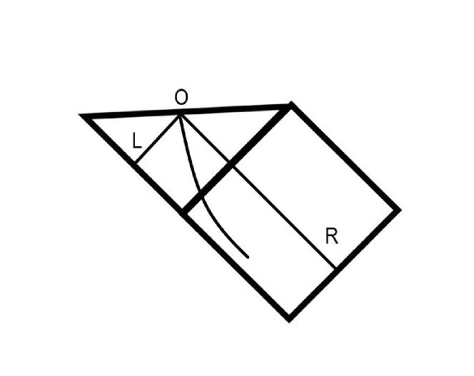
Figure 1: Trajectory of an observer inside a black hole and his individual horizon.

However, this is not the end of story. There were additional assumptions used in the above references without reservations: (i) an observer falls in a black hole starting from the $R1$ region, but not from the $R2$ region (this is a natural assumption for a realistic observer) and (ii) he/she moves along the geodesic path. If one of these requirements (or both) is violated, the answer is to be modified (see below). This is illustrated in Fig.1 showing an observer falling into a singularity and some of light-cones. The part of space-time which can be seen by the observer lies within the past light cone with the vertex at the point $O$ where he/she hits the singularity at some time $t_{s}$. Any events outside this light cone cannot be seen by the observer. So, we can treat this cone as an individual event horizon for the observer in question. Note, that this construction is well known in cosmology, and corresponds to the event horizon of an observer in contracting Universe – it exists due to the fact that (i) lifetime of an observer before the end in cosmological singularity is finite, (ii) the singularity is space-like, so, the range of events which can be seen is finite too. In black hole physics is it important not to mix up this individual horizon (which can be used in description of a free-fall) with standard observer-independent event horizon $r=r_{+}$ absent in cosmology.

In our two-dimension diagram the cross-section of this light cone is in fact two light geodesics directed towards the past. They are represented by the left and right rays in the diagram, so the observer can see events inside this cone at the time of singularity hitting. In the simplest case of the Schwarzschild metric we can explicitly integrate the equation for light geodesics and get the analytical form of the light rays in question. Indeed, integration of equation $ds^{2}=0$ with (23) taken into account gives us

$$\tilde{t}_{R}=\tilde{t}_{s}-r+2\sqrt{r_{+}r}-2r_{+}\log\frac{(\sqrt{r}+\sqrt{r_{+}})}{\sqrt{r_{+}}}\text{,}$$ (42)

$$\tilde{t}_{L}=\tilde{t}_{s}-r+2\sqrt{r_{+}r}+2r_{+}\log\frac{(\sqrt{r_{+}}-\sqrt{r})}{\sqrt{r_{+}}}.$$ (43)

Here, subscripts ”L” and ”R” refer to the left and right rays, respectively. The constant of integration is chosen to ensure that $\tilde{t}=\tilde{t}_{s}$ at $r=0$.

The zone of events which an observer can see before crash into the singularity is given by the interior of the corresponding light cone. For a given $r$, it is given by inequality $\tilde{t}_{L}\leq\tilde{t}\leq\tilde{t}_{R}$. Clearly, for a fixed $r$ we have $\tilde{t}_{R}\to\infty$ if $\tilde{t}_{s}\to\infty$

At this point we remind a reader that any massive particle moving from $R_{1}$ zone into $T$ zone along a geodesic has $\varepsilon>0$. Now, let an observer come from $R_{1}$, being equipped with some engine. Let him turn it on in the point $r$ under the horizon in the $T$ region in such a way that he sits on the trajectory $\varepsilon=0.$ He turns the engine off afterwards, thus making a transition from the geodesic trajectory with $\varepsilon>0$ to the one with $\varepsilon=0$. Then, the Lemaître time from $r$ to singularity is given by (41).

Let $r\rightarrow r_{+}$. Then, this time diverges in accordance with (43). In the point where a particle (astronaut) hits a singularity, we have in (42), (43) $\tilde{t}_{s}\rightarrow\infty$. In doing so, the trajectory of an astronaut bends more and more to the horizon, when $r$ is taken to be closer and closer to $r_{+}$. And, the part of the external Universe in the $R_{1}$ region becomes more and more visible (see Fig.2)

Figure 2: Schematic picture of trajectories of an astronaut changing his path to the E=0 trajectory.

Thus, although the future history of the Universe, accessible to an observer for each astronaut with a rocket, is finite, this part is not limited by some fundamental restrictions. It is limited by the power of the engine required to change an initial trajectory and sit on the trajectory $\varepsilon=0$. It is also limited by the ability of the observer to survive under enormous acceleration caused by this engine: the more powerful is the engine (provided the observer survives during its work), the bigger slope of the $\varepsilon=0$ to the horizon be, and the bigger part of the future of the Universe the observer will see. In other words, each concrete observer sees only a finite part of the future but this part can be expanded without restrictions. One can call this situation ”an observer sees the whole future of the Universe in a weak sense”.

In the limit under discussion the trajectory $\varepsilon=0$ would coincide with the horizon but the only physical object which can reach it there is a light ray (or any another beam of massless particle). Since both velocities $v_{p}=1$ and $v=1$ (as is explained in this Section above), it is seen from (28) that the coordinate $T$ is a constant and so is the radial coordinate $r=r_{+}$ - the beam stays at the horizon forever! However, a realistic photon emitted exactly at the horizon will experience redshift growing exponentially with the Lemaître time along , so the validity of the geometric optics approach becomes questionable and requires separate treatment.

Consider again the view seen by an infalling astronaut. The singularity lies in absolute future, so an astronaut cannot see it. The right ray OR comes from the outer part of Universe from which the astronaut arrived. The astronaut can see it in point O only where this ray hits the singularity. Meanwhile, the ray OL comes from the $R2$ region (”mirror world”). It is inaccessible to the outer observer in region $R1$ but an astronaut in the $T$ region, i.e. inside a black hole, can see it. If there exists the left $R$ region ($R2$) from which information is allowed to propagate, an astronaut can see corresponding events. If there is no such a region (say, in the case of collapse), an astronaut, at least, can see light emitted by the surface of the collapsing star ahead of him (see Ref. Hamilton for details). He can also see the right horizon (which is called a true horizon in Hamilton ) looking in the backward direction, the redshift being finite.

IX Two strategies of an astronaut

The unboundedness of the Lemaître time in free fall into a black hole has one more interesting feature, if we consider not a view of the ”outer” world for an observer, but ask the question is it possible for the astronaut under discussion to communicate with it. Evidently, a communication with any object staying permanently outside the horizon becomes impossible once the astronaut crosses horizon (in fact, even earlier). However, what about objects falling into the black hole? We do not consider here this question in detail, but illustrate with the simplest example of an object with constant spatial Lemaître coordinate $\rho$. A particle with $\rho=\rho_{i}$ reaches the singularity at $\tilde{t}_{1}=\rho_{i}$. If $\tilde{t}_{1}<\tilde{t}_{s}$, the particle in question will pass through the astronaut on the way to singularity. So that, if $\tilde{t}_{s}$ is very big, particles with rather big $\rho$ can still pass near the astronaut in question and could literally touch him/her by hand. Since two both participants (an astronaut and a particle) meet at the same point, the possibility of mutual communication is evident at least till this point which occurs somewhere under the horizon. So that, if $\tilde{t}_{s}$ is very large, more and more free falling observers with bigger and bigger $\rho=const$ are able not only to see the astronaut but mutually communicate!

So, if one uses an engine near the horizon to make $\varepsilon=0$, this helps in achieving two goals at once: maximizing proper time till the singularity and maximizing the possible future of the Universe seen during this fatal fall. We should remark, however, that if the horizon is already passed, and the observer is in $T$ region, these two goals may require different strategies. For example, suppose that the observer inside the horizon found himself at a trajectory with $\varepsilon=0$, but some fuel remains. Is it reasonable to use the fuel more? If we want to make the proper time before hitting singularity as large as possible, the answer is obviously ”no” – the trajectory with $\varepsilon=0$ is optimal. But what about the Lemaître time till the singularity?

The time from some initial $r=r_{0}$ to the singularity $r=0$ is given by (40) with $r=r_{0}$. Under the horizon the integrand is positive, $v>v_{p}$ (see discussion after eq. (39)). Therefore, the bigger $v_{p},$ the bigger is the Lemaître time. So, the astronaut should use the remaining fuel – the fight against gravity makes sense! Ironically, not for the fighter – his proper time till singularity decreases while Lemaître time increases.

Using the results below Eq.(39) we may also note that if an astronaut understands that he/she is actually on the trajectory with $\varepsilon<0$ and wants to achieve the maximum possible proper time, it is necessary to decrease $v_{p}$ in order to reach $\varepsilon=0$. On the contrary, such an astronaut should increase $v_{p}$ as much as possible to maximize the Lemaître time (allowing to see more future of the outer word).

In other words, a researcher inside the horizon should pay by the time of his own life for satisfying his curiosity!

X Conclusions

In our paper we have considered two strategies for an observer falling into a spherically symmetric black hole. The observer may try to maximize either the proper time (this is the case usually considered in textbooks) or the Lemaître time. The latter goal allows the observer to see as much future history of the Universe as possible. These two different goals may or may not lead to different strategies. Of course, they coincide for an observer in the outer region — switching on the engine the observer could ( if the engine is powerful enough) avoid entering inside the horizon. Then, both the proper and Lemaître lifetimes tend to infinity. At the horizon these two goals still require the same action — use the engine us much as possible getting the biggest possible positive peculiar velocity. In the unreachable limit this strategy would turn the energy of the observer to zero, maximizing the proper time to the singularity. Simultaneously, this would lead to peculiar velocity of the observer equal to the speed of light and the Lemaître time to singularity equal to infinity. So, an astronaut with powerful engine which succeeds in ( almost) maximizing the proper lifetime will see as, a “bonus”, (almost) complete future history of the outer world.

Let, being already inside the horizon, the observer decide to live as much as possible and, thus, to maximize the proper time till the singularity. Then, the best strategy, according to (13) consists in reaching the zero energy and turning the engine off afterwards. If, however, the observer would like to see as much future of the outer world as possible, the strategy is to maximize the peculiar velocity (see equation (40)). This means that such a curious observer should use all the power of the engine and not switch it off deliberately. The closer $v_{p}$ is to the unreachable speed of light, the bigger part of future such an observer can see. Such an observer increasing his peculiar velocity as much as possible under the horizon would have large negative $\varepsilon$ (see formula (38), where the numerator is finite and negative for this case, while the denominator is very close to zero for $v_{p}\approx 1$). Then, it follows from (13) with very big $\left|\varepsilon\right|$ that this remote future will pass almost instantly by observer’s own clock between the initial point and the singularity. We would like to stress that there is intimate connection between some properties of motion and metric. Namely, when a point where an astronaut begins to follow the line with $\varepsilon=0$ approaches the horizon, the Lemaître time diverges and the part of the outer universe available for an astronaut increases.

In the present methodological paper we considered an idealized situation and did not take into account details presented in any realistic scenarios. For example, any realistic engine has a finite power, so reaching the trajectory with $\varepsilon=0$ exactly at horizon is impossible. When precisely it is better to switch the engine on, requires a special calculations. More realistic model should also include the fact that an engine works not instantly, but rather gives a finite acceleration. We leave such more technical questions to a separate investigation.

Our consideration applies to any spherically symmetric metric with a simple (nonextremal) horizon, which is static outside it and homogeneous inside, and to any metric theory of gravitation provided particles in the absence of external forces move along geodesics.

- (1) A. V. Toporensky, O. B. Zaslavskii, Zero-momentum trajectories inside a black hole and high energy particle collisions, Journal Cosmol. Astropart. Physics 12 (2019) 063. [arXiv:1808.05254].
- (2) S. Krasnikov, Falling into the Schwarzschild black hole. Important details, Gravitation and Cosmology 14 (2008) 362, [arXiv:0804.3619]
- (3) A. A. Grib, Yu. V. Pavlov, Is it possible to see the infinite future of the Universe when falling into a black hole? Usp.Fiz.Nauk 179:279-283,2009 (Phys.-Usp. 52 257, 2009), [arXiv:0906.1442].
- (4) I. D. Novikov, Note on the space-time metric inside the Schwarzschild singular sphere, Sov. Astr. - AJ, 5, 423 (1961), (Astron. Zh. 38, 564 (1961)).
- (5) V. P. Frolov and I. D. Novikov, Physics of Black Holes (Kluwer Academic, Dordrecht, 1998).
- (6) I. D. Novikov, R- and T-Regions in Space-Time with Spherically Symmetric Space, Soobshch. GAISh 132, 43 (1964) [Gen. Relativ. Gravit. 33, 2259 (2001)].
- (7) G. F. Lewis and J. Kwan, NoWay Back: Maximizing Survival Time Below the Schwarzschild Event Horizon, Publ. of the Astron. Soc. of Australia, 2007, 24, 46–52, [arXiv:0705.1029].
- (8) I. D. Novikov, Black holes and the Universe, Cambridge University Press, Cambridge 1995.
- (9) Painlevé, P.: La mécanique classique et la théorie de la relativité, C. R. Acad. Sci. (Paris) 173, 677 (1921).
- (10) Gullstrand, A. Allgemeine Lösung des statischen Einkörperproblems in der Einsteinschen Gravitationstheorie, Arkiv. Mat. Astron. Fys. 16 (8), 1 (1922)
- (11) A. J. S. Hamilton and J. P. Lisle, The river model of black holes, Am. J. Phys. 76 519, 2008, [arXiv:gr-qc/0411060].
- (12) A V Toporensky, O B Zaslavskii and S B Popov, Unified approach to redshift in cosmological/black hole spacetimes and synchronous frame. Eur. J. Phys. 39, 015601 (2018), [arXiv:1704.08308]
- (13) L. D. Landau and E. M. Liefshitz, The Classical Theory of Fields Pergamon Press, New York (1971).
- (14) C. W. Misner, K. S. Thorne, and J. A. Wheeler, Gravitation, Freeman, San Francisco (1973).
- (15) A. V. Toporensky, O. B. Zaslavskii, Redshift of a photon emitted along the black hole horizon, Eur. Phys. J. C (2017) 77:179, [arXiv:1611.09807].
- (16) A. J. S. Hamilton and G. Polhemus, Stereoscopic visualization in curved spacetime: seeing deep inside a black hole, New J. Phys. 12 (2010) 123027.