Photon-Photon Interactions in Dynamically Coupled Cavities

Abstract

We study theoretically the interaction between two photons in a nonlinear cavity. The photons are loaded into the cavity via a method we propose here, in which the input/output coupling of the cavity is effectively controlled via a tunable coupling to a second cavity mode that is itself strongly output-coupled. Incoming photon wave packets can be loaded into the cavity with high fidelity when the timescale of the control is smaller than the duration of the wave packets. Dynamically coupled cavities can be used to avoid limitations in the photon-photon interaction time set by the delay-bandwidth product of passive cavities. Additionally, they enable the elimination of wave packet distortions caused by dispersive cavity transmission and reflection. We consider three kinds of nonlinearities, those arising from $\chi^{\scriptscriptstyle(2)}$ and $\chi^{\scriptscriptstyle(3)}$ materials and that due to an interaction with a two-level emitter. To analyze the input and output of few-photon wave packets we use a Schrödinger-picture formalism in which travelling-wave fields are discretized into infinitesimal time-bins. We suggest that dynamically coupled cavities provide a very useful tool for improving the performance of quantum devices relying on cavity-enhanced light-matter interactions such as single-photon sources and atom-like quantum memories with photon interfaces. As an example, we present simulation results showing that high fidelity two-qubit entangling gates may be constructed using any of the considered nonlinear interactions.

I Introduction

Photons make excellent flying qubits due to the low decoherence and loss associated with their transport over standard telecommunication fibers. It therefore seems unavoidable that they will play a key role as carriers of quantum information for secure communication networks and distributed quantum computing [1]. The lack of direct interactions between photons makes it very challenging to perform universal quantum information processing using photonic qubits. Indirect interactions may be mediated by materials with optical nonlinearities but these are usually very weak at optical frequencies. Nevertheless, progress in the design and fabrication of nanocavities with very small mode volumes and very large lifetimes [2, 3, 4, 5, 6] has reduced the optical energy required to observe nonlinear interactions close to the single-photon level. To fully exploit the enhanced light-matter interaction inside the cavity, it is necessary for the entire energy of an incoming wave packet to reside in the cavity throughout its lifetime. However, delay-bandwidth trade-offs [7] put bounds on the energy from an incoming wave packet that can reside inside a passive cavity throughout its lifetime. For instance, a rising exponential wave packet may be absorbed completely into a cavity, but only for an infinitesimal time, such that the average energy is smaller than the total incoming energy. The delay-bandwidth limit may be broken using active controls to modify the cavity-waveguide coupling at a timescale smaller than the wave packet temporal width. Such dynamically coupled cavities have been demonstrated in photonic crystals [8] and ring resonators [9]. These demonstrations used short optical pump pulses to generate electric charge carriers in the semiconductor material forming the cavities. The free carrier absorption loss associated with this method degrades the intrinsic quality factor, $Q_{L}$, which motivates the search for an alternative approach.

Here, we propose a method to achieve dynamic coupling that uses the parametric nonlinearity of cavity materials ($\chi^{(2)}$ or $\chi^{(3)}$) and therefore avoids loss.

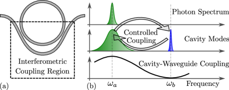
Figure 1: (a) Ring resonator interferometrically coupled to a waveguide. (b) Spectra of the incoming photon wave packet (top), cavity resonances coupled via external control fields (center), and cavity-waveguide coupling rate (bottom).

Two strong optical control fields may couple two cavity modes via so-called Bragg-scattering four-wave-mixing (FWM) in $\chi^{(3)}$-materials [10, 11, 12] and a single control field may do the same in a $\chi^{(2)}$ material [13, 5], as illustrated with arrows in Fig. 1b. If the cavity is interferometrically coupled to a waveguide [14] (see Fig. 1a), one of the cavity modes may be strongly coupled (green mode in Fig. 1b) whereas the other may be completely decoupled from the waveguide (blue mode in Fig. 1b). External control over the coupling between the cavity modes therefore introduces a time-dependent effective coupling between the decoupled mode and the waveguide [12]. In other words, photons may be loaded in and out of the decoupled mode via the strongly coupled mode due to their time-dependent mutual coupling.

We succinctly review a Schrödinger-picture, discrete-time formalism for treating input and output from optical cavities (equivalent to the well-known Heisenberg-picture input/output formalism), and show how it can be used to treat the input/output of one- and two-photon wave packets into and out of dynamically coupled nonlinear cavities. We suggest that dynamically coupled cavities would be useful for a range of quantum applications relying on cavity-enhanced light-matter interaction, and specifically use the formalism to calculate the fidelity of two-qubit gates for travelling-wave photons.

This article is organized as follows: Section II describes the discrete-time formalism and Section III elucidates the Hamiltonians that describe our nonlinear cavity modes. In Section IV we consider the linear regime and examine the dynamics of the cavity modes under the controlled coupling. In Section V we present analytic solutions for the control fields required to absorb and emit wave packets with predefined shapes and consider a specific example in which the wave packets are Gaussian. Section VI contains a description of three types of nonlinear interactions, $\chi^{(2)}$, $\chi^{(3)}$, and two-level emitters (TLEs), and considers their application to controlled-phase (c-phase) gates. Finally, we conclude with a discussion of the limitations of our model and suggest other quantum applications that could benefit from dynamically coupled cavities.

II Discrete-Time Formalism

In our analysis of the dynamics of photons scattering off a system driven by external control fields we discretize the traveling-wave field into time-bins of duration $\Delta t$ as illustrated in Fig. 2 [15, 16, 17].

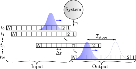
Figure 2: Illustration of the discrete time formalism. The time-axis for the travelling-wave field is divided into discrete bins and time evolution is modeled by shifting the time-axis from left to right. The system interacts with one time bin at a time, modelling a point-interaction with the field as is standard in the input/output formalism for quantum systems.

The time-axis may be thought of as a conveyor belt and time evolution corresponds to dragging this conveyor belt past the fixed system one bin at a time. The discretization involves introducing new field operators

$$\hat{w}(t_{k})=\hat{w}(k\Delta t)\equiv\frac{\hat{w}_{k}}{\sqrt{\Delta t}}\;\;\;\mbox{with}\;\;\;[\hat{w}_{j},\hat{w}_{k}^{\dagger}]=\delta_{jk},$$ (1)

where $\hat{w}(t_{k})$ is the continuous-time annihilation operator that removes a photon from the waveguide at time $t_{k}$. The operator $\hat{w}_{k}$ is the discrete-time counterpart of $\hat{w}(t_{k})$ that removes a photon from the $k^{\mbox{\scriptsize{th}}}$ time-bin. The factor of $1/\sqrt{\Delta t}$ allows $\hat{w}(t_{k})$ to have the canonical commutation relation, $[\hat{w}(t_{j}),\hat{w}^{\dagger}(t_{k})]\!=\!\delta(t_{j}-t_{k})$, as $\Delta t\rightarrow 0$.

For a single-photon input with a wave packet described by $\xi_{\rm{in}}(t)$, the continuous and discrete descriptions are

$$|{\psi_{\rm{in}}}\rangle=\int_{0}^{T}\!\!dt\xi_{\rm{in}}(t)\hat{w}^{\dagger}(t)|{\emptyset}\rangle\approx\sum_{k=1}^{N}\sqrt{\Delta t}\xi^{\rm{in}}_{k}\hat{w}_{k}^{\dagger}|{\emptyset}\rangle,$$ (2)

in which $\int_{0}^{T}|\xi_{\rm{in}}(t)|^{2}=1$ so the state is normalized and $|{\emptyset}\rangle$ denotes the vacuum state of the waveguide. At any time step, $n$ (see Fig. 2), a photon in bin $k$ is referred to as an input photon if $k>n$ and we write the corresponding state of the field as $\hat{w}_{k}^{\dagger}|{\emptyset}\rangle\!\equiv\!|{1_{k}}\rangle$. Similarly, if $k\leq n$ the photon is referred to as an output photon and we denote the corresponding state of the field by $|{\mathbf{1}_{k}}\rangle$.

The system depicted in Fig. 2 consists of a nonlinear multimode cavity. We consider up to three cavity modes of which only one will be coupled to the waveguide and another may be coupled to a two-level emitter. Linear coupling between cavity modes will be implemented by nonlinear interactions with classical control fields. The nonlinear coupling between the photons will originate either from the bulk nonlinearity of the cavity material or an interaction with a TLE. The waveguide-coupled mode is denoted the “auxiliary” cavity mode (oscillating at $\omega_{a}$), and will be used to load and unload photons into and out of the “primary” cavity mode (oscillating at $\omega_{b}$). A third “tertiary” cavity mode (oscillating at $\omega_{c}$), if used, will be coupled to the primary mode and potentially to a TLE.

We use the Schrödinger-picture to derive equations of motion for the time-dependent state coefficients. The unitary time evolution operator describing one time step from $t_{n-1}$ to $t_{n}$ in Fig. 2 is

$$\hat{U}_{n}=\exp\Big{(}\!-\frac{i}{\hbar}\hat{H}_{n}\Delta t\Big{)}=\sum_{m=0}^{\infty}\frac{1}{m!}\Big{(}\!-\frac{i}{\hbar}\hat{H}_{n}\Delta t\Big{)}^{\!m},$$ (3)

such that the updated state is

$$|{\psi_{n}}\rangle=\hat{U}_{n}|{\psi_{n-1}}\rangle,$$ (4)

with $\hat{H}_{n}$ being the Hamiltonian describing the system and its interaction with the waveguide at time-step $n$. In the next section we explain the model used to describe the system and their interaction with the waveguide and additional loss channels.

III Model

A model for the complete system consists of a specification of the Hamiltonian in Eq. (3). It is assumed that the interaction between the system and waveguide occurs at a singular spatial point, which corresponds to interaction only with bin $n$ at time $t_{n}$. It is therefore convenient to think of $N$ different Hamiltonians, $\hat{H}_{n}$, each acting only during the $n^{\mbox{\scriptsize{th}}}$ time step.

The self-energy terms of the system Hamiltonian in a rotating frame (also know as the interaction picture, see Appendix A) are

$$\hat{H}_{0}=\hbar\delta_{a}\hat{a}^{\dagger}\hat{a}+\hbar\delta_{b}\hat{b}^{\dagger}\hat{b}+\hbar\delta_{c}\hat{c}^{\dagger}\hat{c}+\hbar\delta_{e}\hat{\sigma}_{z},$$ (5)

where $\hat{a}$, $\hat{b}$, and $\hat{c}$ annihilate, respectively, a photon from the auxiliary cavity mode ($a$), primary mode ($b$), and tertiary mode ($c$). The operator $\hat{\sigma}_{z}\!=\!|{e}\rangle\langle{e}|$, with $|{e}\rangle$ being the excited state of a TLE coupled to mode $c$. The detunings, $\delta_{n}$, are used to account for discrepancies between energy levels of the system and the incoming photons and control fields as described in Appendix A.

Coupling between the waveguide and the auxiliary cavity mode is described by the Hamiltonian [16]

$$\hat{H}_{n}^{\rm{cav-wg}}=i\hbar\sqrt{\frac{\gamma}{\Delta t}}\Big{(}\hat{a}^{\dagger}\hat{w}_{n}-\hat{a}\hat{w}_{n}^{\dagger}\Big{)},$$ (6)

where $\gamma$ is the coupling rate.

As mentioned above, a dynamic cavity-waveguide coupling is established by coupling two cavity modes, one strongly coupled and one decoupled from the waveguide, via nonlinear interactions driven by external control fields. In materials with a third order nonlinearity, $\chi^{(3)}$, the coupling Hamiltonian is

$$\hat{H}_{n}^{\rm{cav-cav}}=\hbar\chi_{3}\Big{(}\hat{p}_{1}^{\dagger}\hat{p}_{2}\hat{a}^{\dagger}\hat{b}+\hat{p}_{2}^{\dagger}\hat{p}_{1}\hat{b}^{\dagger}\hat{a}\Big{)},$$ (7)

The operators $\hat{p}_{1}$ and $\hat{p}_{2}$ annihilate photons from two pump modes far detuned from modes $a$, $b$, and $c$. The pump fields are treated classically by taking expectation values and making the substitution [18]

$$\chi_{3}\langle\hat{p}_{2}^{\dagger}\hat{p}_{1}\rangle\!=\!\chi_{3}\alpha_{2}^{*}(t_{n})\alpha_{1}(t_{n})\!=\!\Lambda(t_{n}),$$ (8)

where $\alpha_{n}$ is the eigenvalue of the annihilation operator $\hat{p}_{n}$ and $\Lambda(t_{n})$ is the complex-valued control field. With the classical control field, Eq. (7) reads

$$\hat{H}_{n}^{\rm{cav-cav}}=\hbar\Big{(}\Lambda_{n}^{*}\hat{a}^{\dagger}\hat{b}+\Lambda_{n}\hat{b}^{\dagger}\hat{a}\Big{)},$$ (9)

which now describes a linear coupling between modes $a$ and $b$ driven by the time-dependent control field, $\Lambda(t)$. Note that in the case of a TLE nonlinearity, we introduce a second control field, $\Pi(t)$ that couples modes $b$ and $c$ using pump modes $p_{1}$ and another mode $p_{3}$, see Appendix A.

For $\chi^{\scriptscriptstyle(3)}$ materials, we must also include the cross-phase modulation caused by the pump fields on modes $a$, $b$, and $c$ described by the Hamiltonian

$$\hat{H}_{n}^{X\!P\!M\!,p}=\hbar\chi_{3}\sum_{m\!=\!1}^{2}\hat{p}_{m}^{\dagger}\hat{p}_{m}\Big{(}\hat{a}^{\dagger}\hat{a}+\hat{b}^{\dagger}\hat{b}+\hat{c}^{\dagger}\hat{c}\Big{)}~{}\rightarrow\\ 2\hbar|\Lambda_{n}|\Big{(}\hat{a}^{\dagger}\hat{a}+\hat{b}^{\dagger}\hat{b}+\hat{c}^{\dagger}\hat{c}\Big{)},$$ (10)

where we have assumed $\chi_{3}\langle\hat{p}_{2}^{\dagger}\hat{p}_{2}\rangle\!=\!\chi_{3}\langle\hat{p}_{1}^{\dagger}\hat{p}_{1}\rangle\!=\!|\Lambda_{n}|$, which means that the optical energy in each pump mode is identical at all times.

In a $\chi^{\scriptscriptstyle(2)}$ material the cavity-cavity coupling arises from the Hamiltonian

$$\hat{H}_{n}^{\rm{cav-cav}}=\hbar\chi_{2}\Big{(}\hat{p}^{\dagger}\hat{a}^{\dagger}\hat{b}+\hat{p}\hat{b}^{\dagger}\hat{a}\Big{)}.$$ (11)

We assume the frequency separation between modes $a$ and $b$ to be in the GHz range and $\hat{p}$ is therefore the annihilation operator of a radio-frequency (RF) electric field that may be applied using electrodes [5]. Again, we describe it classically by

$$\chi_{2}\langle\hat{p}\rangle\!=\!\chi_{2}\alpha_{p}(t_{n})\!=\!\Lambda_{n}.$$ (12)

The coupling Hamiltonian expressed in terms of the classical control field is therefore given by Eq. (9) for both second- and third-order nonlinear materials. There is no cross-phase modulation term in the Hamiltonian for a $\chi^{\scriptscriptstyle(2)}$ material (unless a DC electric field is applied), so Eq. (10) does not apply in that case.

The Hamiltonian describing the three different types of nonlinear materials are

$$\hat{H}_{\rm{XPM}}\!+\!\hat{H}_{\rm{SPM}} =\hbar\chi_{3}\Big{[}\hat{a}^{\dagger}\hat{a}\hat{b}^{\dagger}\hat{b}+\hat{b}^{\dagger}\hat{b}\hat{c}^{\dagger}\hat{c}\Big{]}~{}+$$

$$\hskip 62.59596pt\frac{\hbar\chi_{3}}{4}\!\sum_{\hat{q}}\!\Big{(}\!\hat{q}^{\dagger}\hat{q}\!-\!1\!\Big{)}\hat{q}^{\dagger}\hat{q}$$ (13a)

$$\hat{H}_{\rm{SHG}} =\hbar\chi_{2}\Big{(}\hat{c}\hat{b}^{\dagger}\hat{b}^{\dagger}+\hat{c}^{\dagger}\hat{b}\hat{b}\Big{)}$$ (13b)

$$\hat{H}_{\rm{TLE}} =\hbar\Big{(}g\hat{c}^{\dagger}\hat{\sigma}_{\!-}+g^{*}\hat{c}\hat{\sigma}_{\!+}\Big{)},$$ (13c)

where $\hat{q}\!\in\!\{\hat{a},\hat{b},\hat{c}\}$ in Eq. (13a) and $\hat{\sigma}_{\!-}\!\equiv\!|{g}\rangle\langle{e}|$ and $\hat{\sigma}_{\!+}\!\equiv\!|{e}\rangle\langle{g}|$ in Eq. (13c) with $|{g}\rangle$ being the ground state and $|{e}\rangle$ the excited state of the TLE. Note that not all possible combinations of modes are considered in Eq. (13), but only those included in the protocols for photon-photon interactions that we consider here.

IV Linear Dynamics

In this section we derive equations of motion including only the linear dynamics. We start with the simplest case of one photon coupling to one cavity mode to built intuition about the derivation procedure. Then, we consider one photon coupling to a cavity with two modes, and finally two photons coupling to a cavity with two modes. Having derived equations of motion in the linear regime, it is fairly straight forward to add nonlinear interactions and make the appropriate additions to the equations, which we do in Section VI.

IV.1 One Cavity Mode - One Photon

Let us begin by considering a single input photon coupling to one cavity mode. The relevant terms of the Hamiltonian are

$$\hat{H}_{n}^{(1)}=\hbar\delta_{a}\hat{a}^{\dagger}\hat{a}+i\hbar\sqrt{\frac{\gamma}{\Delta t}}\Big{(}\hat{a}^{\dagger}\hat{w}_{n}-\hat{a}\hat{w}_{n}^{\dagger}\Big{)}.$$ (14)

Keeping only terms to first order in $\Delta t$, the corresponding time-evolution operator is

$$\hat{U}_{n}^{(1)}\approx\hat{\mathbb{I}}+\sqrt{\gamma\Delta t}\Big{(}\hat{a}^{\dagger}\hat{w}_{n}-\hat{a}\hat{w}_{n}^{\dagger}\Big{)}~{}-\\ \frac{\gamma}{2}\Delta t\hat{a}^{\dagger}\hat{a}\hat{w}_{n}\hat{w}_{n}^{\dagger}-i\delta_{a}\Delta t\hat{a}^{\dagger}\hat{a}.$$ (15)

The state at time step $n$ is

$$|{\psi_{n}}\rangle=\!\!\sum_{k=n+1}^{N}\!\!\xi^{\rm{in}}_{k}\sqrt{\Delta t}|{0}\rangle|{1_{k}}\rangle~{}+\\ \sum_{k=1}^{n}\xi^{\rm{out}}_{k}\sqrt{\Delta t}|{0}\rangle|{\mathbf{1}_{k}}\rangle+\psi_{1}(n)|{1}\rangle|{\emptyset}\rangle,$$ (16)

where $\xi^{\rm{in}}_{k}\!=\!\xi_{\rm{in}}(t_{k})$ describes the input wave packet. The states $|{0}\rangle|{1_{k}}\rangle$ and $|{0}\rangle|{\mathbf{1}_{k}}\rangle$ correspond to an empty cavity and a photon in bin $k$ on the input ($k>n$) and output ($k\leq n$) side, respectively. The state corresponding to a photon in the cavity has the coefficient $\psi_{1}(n)$. In Appendix B we derive the equation of motion for $\psi_{1}(t)$ and the input-output relation connecting $\xi_{\rm{out}}(t)$ to $\xi_{\rm{in}}(t)$

$$\dot{\psi}_{1}(t) =-\Big{(}i\delta_{a}+\frac{\gamma}{2}\Big{)}\psi_{1}(t)+\sqrt{\gamma}\xi_{\rm{in}}(t)$$ (17a)

$$\xi_{\rm{out}}(t) =\xi_{\rm{in}}(t)-\sqrt{\gamma}\psi_{1}(t).$$ (17b)

These equations have the same form as those derived classically using arguments of energy conservation and time-reversal symmetry [19]. They also have the same form as the Heisenberg equations of motion of the usual input-output formalism [20].

IV.2 Loss

At this stage we consider the effect of loss. It may be conveniently modeled using an additional waveguide with a vacuum input. If the annihilation operator that removes a photon from the loss channel at time $t_{n}$ is $\hat{l}_{n}$, then the time-evolution operator has the additional terms

$$\hat{U}_{n}^{\rm{loss}}=\sum_{\hat{q}}\Big{[}\sqrt{\gamma_{L}\Delta t}\big{(}\hat{q}^{\dagger}\hat{l}_{n}-\hat{q}\hat{l}_{n}^{\dagger}\big{)}-\frac{\gamma_{L}}{2}\Delta t\hat{q}^{\dagger}\hat{q}\hat{l}_{n}\hat{l}_{n}^{\dagger}\Big{]},$$ (18)

where $\hat{q}$ represents all the cavity modes (we assume they have identical loss rates, $\gamma_{L}$). If we ignore all states of the loss channel except the vacuum, Eq. (18) shows that a term, $-m\gamma_{L}/2$, is added to all loss terms (with $m$ photons in the cavity mode), such that the loss term in Eq. (17a) would have the coefficient $-(\gamma\!+\!\gamma_{L})/2$. We therefore define the total coupling rate, $\Gamma\!=\!\gamma\!+\!\gamma_{L}$. Noise photons injected into the system from the loss channel due to vacuum fluctuations at finite temperatures is neglected in this treatment.

Ignoring all states in the loss channel except the vacuum, $|{\emptyset}\rangle_{{}_{\!L}}$, our total state is $|{\psi}\rangle|{\emptyset}\rangle_{{}_{\!L}}$. It will not be normalized due to the finite probability of finding photons in the loss channel. We may, however, consider a heralded state, $|{\psi_{M}}\rangle$, corresponding to a measurement revealing that the loss channel was, in fact, in the state $|{\emptyset}\rangle_{{}_{\!L}}$

$$|{\psi_{M}}\rangle=\frac{\big{(}|{\emptyset}\rangle_{{}_{\!L}}{}_{{}_{L}}\!\langle{\emptyset}|\big{)}|{\Psi}\rangle}{\sqrt{\big{\langle}{\Psi|\big{(}|{\emptyset}\rangle_{{}_{\!L}}{}_{{}_{L}}\!\langle{\emptyset}|\big{)}|\Psi}\big{\rangle}}}=\frac{|{\psi}\rangle}{\sqrt{1-P_{L}}},$$ (19)

where $|{\Psi}\rangle\!=\!|{\psi}\rangle|{\vartheta}\rangle_{{}_{\!L}}$ is the normalized full state, $|{\vartheta}\rangle_{{}_{\!L}}$ is the state of the loss channel, and the probability of losing at least one photon is $P_{L}\!=\!1\!-\!\big{|}\big{\langle}{\psi|\psi}\big{\rangle}\big{|}^{2}$. The overlap between the output state and some desired state $|{\Phi}\rangle$ is often used as a metric for the precision with which systems are able to implement desired quantum state transformations. Here, we can define

$$\langle\Psi_{\rm{out}}^{(n)}|\Phi\rangle=\sqrt{F_{n}}e^{i\theta_{n}},$$ (20)

where $F_{n}$ is the state fidelity and $\theta_{n}$ the phase of the overlap with $n\!=\!\{1,2\}$ input photons. With the definition of states as superpositions over temporal modes in Eq. (2) the overlaps in Eq. (20) are

$$\langle\Psi_{\rm{out}}^{(1)}|\Phi\rangle =\int_{0}^{T}\!\!\!\xi_{\rm{out}}(t)\xi_{\Phi}(t)^{*}dt$$ (21)

$$\langle\Psi_{\rm{out}}^{(2)}|\Phi\rangle =\int_{0}^{T}\!\!\!\int_{0}^{T}\!\!\!\xi_{\rm{out}}(t_{1},t_{2})\xi_{\Phi}(t_{1})^{\!*}\xi_{\Phi}(t_{2})^{\!*}dt_{1}dt_{2},$$ (22)

where we assumed that the desired state for two-photon inputs is a separable state with the same superposition over temporal modes for both photons. Note that, for a single-photon input,

$$1-P_{L}=\langle\psi^{(1)}_{\rm{out}}|\psi^{(1)}_{\rm{out}}\rangle=\int_{0}^{T}\!\!\!|\xi_{\rm{out}}(t)|^{2}dt,$$ (23)

which illustrates that when the total state, $|{\psi}\rangle|{\emptyset}\rangle_{{}_{\!L}}$ is not normalized, it means that the integral over $|\xi_{\rm{out}}|^{2}$ is smaller than one.

If we are only interested in states without lost photons, $|{\Phi}\rangle\!=\!|{\phi}\rangle|{\emptyset}\rangle_{{}_{\!L}}$, the fidelity may be written as

$$F_{n}=\big{|}{}_{{}_{L}}\!\langle{\emptyset}|\langle\psi_{\rm{out}}^{(n)}|\phi\rangle|{\emptyset}\rangle_{{}_{\!L}}\rangle\big{|}^{2}\!=(1\!-\!P_{L})\big{|}\langle\psi^{(n)}_{{\rm{out}},M}|\phi\rangle\!\big{|}^{2}.$$ (24)

Eq. (24) allows us to define a conditional state fidelity

$$\overline{F}_{n}=\frac{1}{1-P_{L}}F_{n},$$ (25)

which separates the infidelity due to loss from that originating from other sources. This becomes useful later, when we show that dynamically controlled cavities may emit photons into wave packets with a desired shape by reducing the overall emission probability.

In the following sections, we include the loss term proportional to $\gamma_{L}$ in all the equations of motion.

IV.3 Two Cavity Modes - One Photon

For two cavity modes and a $\chi^{(3)}$ material, the Hamiltonian describing the linear dynamics is

$$\hat{H}_{n}^{(2)}=\hbar\delta_{a}\hat{a}^{\dagger}\hat{a}\!+\!\hbar\delta_{b}\hat{b}^{\dagger}\hat{b}\!+\!i\hbar\sqrt{\frac{\gamma}{\Delta t}}\Big{(}\hat{a}^{\dagger}\hat{w}_{n}-\hat{a}\hat{w}_{n}^{\dagger}\Big{)}~{}+\\ \hbar\Big{(}\Lambda_{n}^{*}\hat{a}^{\dagger}\hat{b}+\Lambda_{n}\hat{b}^{\dagger}\hat{a}\Big{)}+2\hbar|\Lambda_{n}|\Big{(}\hat{a}^{\dagger}\hat{a}+\hat{b}^{\dagger}\hat{b}\Big{)}.$$ (26)

The corresponding time-evolution operator is

$$\hat{U}_{n}^{(2)}\approx\hat{\mathbb{I}}+\sqrt{\gamma\Delta t}\Big{(}\hat{a}^{\dagger}\hat{w}_{n}-\hat{a}\hat{w}_{n}^{\dagger}\Big{)}~{}-\\ \frac{\gamma}{2}\Delta t\hat{a}^{\dagger}\hat{a}\hat{w}_{n}\hat{w}_{n}^{\dagger}-i\Delta t\Big{(}\Lambda_{n}^{*}\hat{a}^{\dagger}\hat{b}+\Lambda_{n}\hat{b}^{\dagger}\hat{a}\Big{)}~{}-\\ i\Delta t\big{(}\delta_{a}+2|\Lambda_{n}|\big{)}\hat{a}^{\dagger}\hat{a}-i\Delta t\big{(}\delta_{b}+2|\Lambda_{n}|\big{)}\hat{b}^{\dagger}\hat{b}.$$ (27)

Note that we have omitted the loss terms from Eq. (18), but we will include them in the equations of motion below. The state at time step $n$ is

$$|{\psi_{n}}\rangle=\!\!\sum_{k=n+1}^{N}\!\!\xi^{\rm{in}}_{k}\sqrt{\Delta t}|{00}\rangle|{1_{k}}\rangle+\sum_{k=1}^{n}\xi^{\rm{out}}_{k}\sqrt{\Delta t}|{00}\rangle|{\mathbf{1}_{k}}\rangle~{}+\\ +\psi_{10}(n)|{10}\rangle|{\emptyset}\rangle+\psi_{01}(n)|{01}\rangle|{\emptyset}\rangle,$$ (28)

where $|{01}\rangle\!\equiv\!|{0_{a}}\rangle|{1_{b}}\rangle$ is the state with one photon in mode $b$. In Appendix C we derive the equations of motion for the coefficients $\psi_{10}(t)$ and $\psi_{01}(t)$ along with the input-output relation

$$\dot{\psi}_{10} =-\Big{(}i\delta_{a}+\frac{\Gamma}{2}+i2|\Lambda|\Big{)}\psi_{10}-i\Lambda^{*}\psi_{01}+\sqrt{\gamma}\xi_{\rm{in}}$$ (29a)

$$\dot{\psi}_{01} =-\Big{(}i\delta_{b}+\frac{\gamma_{L}}{2}+i2|\Lambda|\Big{)}\psi_{01}-i\Lambda\psi_{10}$$ (29b)

$$\xi_{\rm{out}} =\xi_{\rm{in}}-\sqrt{\gamma}\psi_{10}.$$ (29c)

Note that we have not explicitly written the time dependence of the functions in Eq. (29).

IV.4 Two Cavity Modes - Two Identical Photons

The analysis becomes significantly more complicated for two input photons so we find it beneficial to map out all the different paths they may take from input to output and the different types of states generated in the process, see Fig. 3.

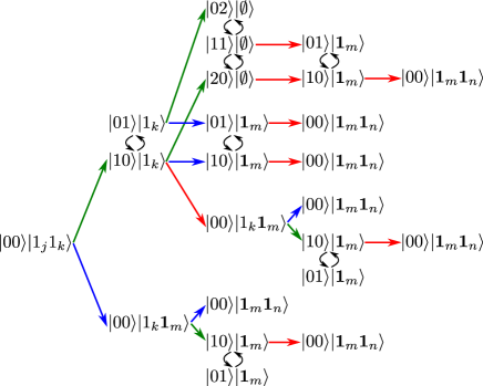
Figure 3: Map of states generated with two cavity modes and two input photons and paths from input to output. Green arrows represent absorption of a photon into mode $a$. Red arrows represent emission into the waveguide in bin $m$. Blue arrows represent a photon passing by the system without interacting in time bin $m$. Black arrows indicate the interaction between modes $a$ and $b$ driven by the external control fields. There are five vertical layers going from left to right.

Let us go through the layers of the map from left to right and write down the dynamical equations governing the expansion coefficients of the states in each layer. The first layer only contains the input state

$$|{\psi_{0}}\rangle=\sqrt{2}\sum_{j=1}^{N}\sum_{k>j}^{N}\xi^{\rm{in}}_{j}\xi^{\rm{in}}_{k}\Delta t|{00}\rangle|{1_{j}1_{k}}\rangle.$$ (30)

Note that the summation over $k$ starts at $j$ in Eq. (30) so that the indistinguishable states $|{1_{j}1_{k}}\rangle$ and $|{1_{k}1_{j}}\rangle$ are only counted once in the summations. In Appendix D we prove that the factor of $\sqrt{2}$ ensures that the state is normalized when the integral of $|\xi_{\rm{in}}(t)|^{2}$ equals 1. We note that derivations of all the equations of motion for coefficients of the Schrödinger picture state in this section may be found in Appendix D.

One of the two photons in layer 1 may be absorbed giving rise to states in layer 2 with one photon in mode $a$ or $b$. The dynamical equations for the coefficients corresponding to these states are

$$\dot{\psi}_{10}^{\rm{ii}} =-\Big{(}i\delta_{a}\!+\!\frac{\Gamma}{2}\!+\!i2|\Lambda|\Big{)}\psi_{10}^{\rm{ii}}-i\Lambda^{\!*}\psi_{01}^{\rm{ii}}+\sqrt{2\gamma}\xi_{\rm{in}}$$ (31a)

$$\dot{\psi}_{01}^{\rm{ii}} =-\Big{(}i\delta_{b}\!+\!\frac{\gamma_{L}}{2}\!+\!i2|\Lambda|\Big{)}\psi_{01}^{\rm{ii}}\!-\!i\Lambda\psi_{10}^{\rm{ii}},$$ (31b)

where we use the superscript ⁱⁱ to signify that the driving term in Eq. (31a) originates from two input photons, which is why it contains a factor of $\sqrt{2}$ relative to Eq. (29a). A convenient feature of the map in Fig. 3 is that the couplings represented by black arrows turn up in the equations of motion as coupling terms proportional to the control field, $\Lambda(t)$, and therefore serves to check whether all the dynamics is included.

The state $|{00}\rangle|{1_{k}\mathbf{1}_{m}}\rangle$ in layer 2 originates from direct passage of one of the input photons, while in layer 3 it originates from absorption and subsequent emission. If the photon remaining on the input side is later absorbed, it gives rise to states $|{10}\rangle|{\mathbf{1}_{m}}\rangle$ and $|{01}\rangle|{\mathbf{1}_{m}}\rangle$ in layer 3 or 4. The dynamical equations for the coefficients corresponding to these states are

$$\dot{\psi}_{10}^{\rm{i}}(\tau,t) \!=\!-\Big{(}i\delta_{a}\!+\!\frac{\Gamma}{2}\!+\!i2|\Lambda(t)|\Big{)}\psi_{10}^{\rm{i}}(\tau,t)~{}-$$

$$\hskip 73.97733pti\Lambda^{*}\psi_{01}^{\rm{i}}(\tau,t)+\sqrt{\gamma}\xi_{\rm{in}}(t)$$ (32a)

$$\dot{\psi}_{01}^{\rm{i}}(\tau,t) \!=\!-\Big{(}i\delta_{b}\!+\!\frac{\gamma_{L}}{2}\!+\!i2|\Lambda(t)|\Big{)}\psi_{01}(\tau,t)~{}-$$

$$\hskip 125.19194pti\Lambda\psi_{10}^{\rm{i}}(\tau,t),$$ (32b)

where the superscript ⁱ signifies that Eq. (32a) is driven by a single input photon. The coefficients $\psi_{10}^{\rm{i}}$ and $\psi_{01}^{\rm{i}}$ are functions of two times, $\tau$ being the initial time at which the state $|{00}\rangle|{1_{k}\mathbf{1}_{m}}\rangle$ was created, and $t\geq\tau$ describing the subsequent evolution of the coefficients. The initial condition of Eq. (32) is $\psi_{10}^{\rm{i}}(\tau,\tau)\!=\!\psi_{01}^{\rm{i}}(\tau,\tau)\!=\!0$ since the system is in state $|{00}\rangle$ at time $\tau$.

States in layer 3 with two photons in the system have coefficients with the following equations of motion

$$\!\dot{\psi}_{20} \!=-\big{(}i2\delta_{a}\!+\!\Gamma+i4|\Lambda|\big{)}\psi_{20}~{}-$$

$$\hskip 93.89418pti\sqrt{2}\Lambda^{\!*}\psi_{11}+\sqrt{2\gamma}\psi_{10}^{\rm{ii}}\xi_{\rm{in}}$$ (33a)

$$\!\dot{\psi}_{11} \!=-\Big{(}i(\delta_{a}\!+\!\delta_{b})+\frac{\Gamma+\gamma_{L}}{2}\!+\!i4|\Lambda|\Big{)}\psi_{11}~{}-$$

$$\hskip 62.59596pti\sqrt{2}\Big{[}\Lambda\psi_{20}\!+\!\Lambda^{\!*}\psi_{02}\Big{]}\!+\!\sqrt{\gamma}\psi_{01}^{\rm{ii}}\xi_{\rm{in}}$$ (33b)

$$\!\dot{\psi}_{02} \!=\!-\big{(}i2\delta_{b}+\gamma_{L}\!+\!i4|\Lambda|\big{)}\psi_{02}\!-\!i\sqrt{2}\Lambda\psi_{11}.$$ (33c)

The initial conditions are $\psi_{20}(0)\!=\!\psi_{11}(0)\!=\!\psi_{02}(0)\!=\!0$.

There are other paths leading to the states $|{10}\rangle|{\mathbf{1}_{m}}\rangle$ and $|{01}\rangle|{\mathbf{1}_{m}}\rangle$ than those described by the dynamics in Eq. (32). It could either be from absorption of the first photon followed by direct passage of the second photon or emission from mode $a$ while the state is $|{20}\rangle|{\emptyset}\rangle$ or $|{11}\rangle|{\emptyset}\rangle$. We use different coefficients for the state originating from these paths because their dynamical equations do not contain driving terms from input photons. The equations are

$$\dot{\psi}_{10}^{\rm{o}}(\tau,t) =-\Big{(}i\delta_{a}\!+\!\frac{\Gamma}{2}+i2|\Lambda(t)|\Big{)}\psi_{10}^{\rm{o}}(\tau,t)~{}-$$

$$\hskip 113.81102pti\Lambda(t)^{\!*}\psi_{01}^{\rm{o}}(\tau,t)$$ (34a)

$$\dot{\psi}_{01}^{\rm{o}}(\tau,t) =-\Big{(}i\delta_{b}\!+\!\frac{\gamma_{L}}{2}+i2|\Lambda(t)|\Big{)}\psi_{01}^{\rm{o}}(\tau,t)~{}-$$

$$\hskip 113.81102pti\Lambda(t)\psi_{10}^{\rm{o}}(\tau,t).$$ (34b)

There are two sets of initial conditions for Eq. (34) depending on whether the dynamics originated from the formation of state $|{10}\rangle|{\mathbf{1}_{m}}\rangle$ or $|{01}\rangle|{\mathbf{1}_{m}}\rangle$ at time $\tau\!=\!m\Delta t$. If the photon started in mode $a$, the initial condition is $\psi_{10}^{\rm{o}}(\tau,\tau)\!=\!1$ and $\psi_{01}^{\rm{o}}(\tau,\tau)\!=\!0$, and we define $L_{10}\equiv\psi_{10}^{\rm{o}}$ and $L_{01}\equiv\psi_{01}^{\rm{o}}$. If the photon started in mode $b$, the initial condition is $\psi_{10}^{\rm{o}}(\tau,\tau)\!=\!0$ and $\psi_{01}^{\rm{o}}(\tau,\tau)\!=\!1$, and we define $M_{10}\equiv\psi_{10}^{\rm{o}}$ and $M_{01}\equiv\psi_{01}^{\rm{o}}$.

Fig. 3 reveals that there are 8 distinct paths from input to output so the coefficient of the output state $|{00}\rangle|{\mathbf{1}_{m}\mathbf{1}_{n}}\rangle$ should contain 8 terms

$$\xi_{\rm{out}}(\tau,t)=\frac{1}{\sqrt{2}}\Big{[}\gamma\psi_{11}(\tau)M_{10}(\tau,t)~{}+\\ \sqrt{2}\gamma\psi_{20}(\tau)L_{10}(\tau)-\sqrt{\gamma}\psi_{01}^{\rm{ii}}(\tau)\xi_{\rm{in}}(\tau)M_{10}(\tau,t)~{}-\\ \sqrt{\gamma}\psi_{10}^{\rm{ii}}(\tau)\xi_{\rm{in}}(\tau)L_{10}(\tau,t)-\sqrt{\gamma}\psi_{10}^{\rm{ii}}(\tau)\xi_{\rm{in}}(t)~{}+\\ \!\gamma\psi_{10}^{\rm{ii}}(\tau)\psi_{10}^{\rm{i}}(\tau\!,t)\!+\!\xi_{\rm{in}}(\tau)\xi_{\rm{in}}(t)\!-\!\sqrt{2\gamma}\xi_{\rm{in}}(\tau)\psi_{10}^{\rm{i}}(\tau\!,t)\Big{]},$$ (35)

where the first term corresponds to the upper path in Fig. 3, the second term to the path immediately below, and so forth. Note that $\tau\leq t$ in Eq. (35) and $\xi_{\rm{out}}(\tau,t)\!=\!\xi_{\rm{out}}(t,\tau)$ follows from the indistinguishability of the photons. The output state is defined as

$$|{\psi_{\rm{out}}}\rangle\equiv\int_{0}^{T}\!\!d\tau\int_{0}^{T}\!\!dt\xi_{\rm{out}}(\tau,t)\hat{w}^{\dagger}(\tau)\hat{w}^{\dagger}(t)|{\emptyset}\rangle,$$ (36)

and the integral of $|\xi_{\rm{out}}(\tau,t)|^{2}$ over $\tau$ and $t$ is 1 (in the absence of loss). To calculate the output state in Eq. (35), we solve the above equations of motion for $N$ different initial conditions corresponding to all the time bins in Fig. 2.

V Absorbing and Emitting Wave Packets via Dynamic Coupling

In this section we find analytic solutions for the control fields that allow absorption and emission of wave packets with known shapes with arbitrarily high fidelity. We consider a specific example of Gaussian wave packets and show by numerical integration of Eq. (29) that the fidelity of the absorption and emission process approaches unity very rapidly as the ratio between the cavity-waveguide coupling, $\gamma$, and the wave packet bandwidth, $\Omega_{\scriptscriptstyle\mathcal{G}}$, increases.

V.1 Absorption

For the absorption process, the boundary conditions of Eq. (29) are $\psi_{10}(0)\!=\!\psi_{01}(0)\!=\!0$. We use a subscript $i$ (for “in”) on the control function, $\Lambda_{i}(t)$. The goal is to determine $\Lambda_{i}(t)$ such that a single incoming photon with wave packet $\xi_{\rm{in}}(t)$ is absorbed into cavity mode $b$. Since $\Lambda_{i}$ is complex-valued, we write it as $\Lambda_{i}(t)\equiv|\Lambda_{i}(t)|\exp[i\phi_{i}(t)]$. In Appendix E we find the solution for a material with a third-order nonlinearity

$$|\Lambda_{i}(t)| =\frac{|f_{i}(t)|e^{-\frac{\gamma_{L}t}{2}}}{|\xi_{\rm{in}}(t)|\sqrt{2\int_{0}^{t}\!f_{i}(s)ds-4|\xi_{\rm{in}}(t)|^{2}e^{\gamma_{L}t}}}$$ (37a)

$$\phi_{i}(t) =-\delta_{b}t-2\int_{0}^{t}\!|\Lambda_{i}(s)|ds-\arg(\xi_{\rm{in}})~{}+$$

$$\hskip 28.45274pt\tan^{-1}\!\bigg{(}\frac{f_{i}\sin(\theta_{i})-g_{i}\cos(\theta_{i})}{f_{i}\cos(\theta_{i})+g_{i}\sin(\theta_{i})}\bigg{)},$$ (37b)

where

$$f_{i}(t) =\Big{(}\frac{\gamma-\gamma_{L}}{2}\xi_{\rm{in}}(t)-\dot{\xi}(t)\Big{)}\xi_{\rm{in}}(t)^{*}e^{\gamma_{L}t}$$ (38a)

$$g_{i}(t) =-2|\Lambda_{i}(t)||\xi_{\rm{in}}(t)|^{2}e^{\gamma_{L}t}$$ (38b)

$$\theta_{i}(t) =-\frac{1}{2}\int_{0}^{t}\!\!\frac{g_{i}(s)}{\int_{0}^{s}\!f_{i}(z)dz}ds.$$ (38c)

Note that we have assumed that $\xi_{\rm{in}}$ does not have a time dependent phase, such that $f_{i}$ and $g_{i}$ are real functions. It is straight forward to generalize this to chirped pulses with time dependent phase by re-defining $f_{i}$ and $g_{i}$. We also assumed $\delta_{a}\!=\!0$ above.

In the case of a material with a second-order nonlinearity there is no cross-phase modulation from the control field, so $g_{i}\!=\!0$ and the solution reduces to

$$|\Lambda_{i}(t)| =\frac{|f_{i}(t)|e^{-\frac{\gamma_{L}t}{2}}}{|\xi_{\rm{in}}(t)|\sqrt{2\int_{0}^{t}\!f_{i}(s)ds}}$$ (39a)

$$\phi_{i}(t) =-\arg(\xi_{\rm{in}}),$$ (39b)

with $f_{i}(t)$ still given by Eq. (38a).

V.2 Emission

Without any driving field, the equations of motion are found by setting $\xi_{\rm{in}}\!=\!0$ in Eq. (29)

$$\dot{\psi}_{10} =\Big{(}-\frac{\Gamma}{2}-i2|\Lambda_{o}|\Big{)}\psi_{10}-i|\Lambda_{o}|e^{-i\phi_{o}}\psi_{01}$$ (40a)

$$\dot{\psi}_{01} =\Big{(}-\frac{\gamma_{L}}{2}-i2|\Lambda_{o}|\Big{)}\psi_{01}-i|\Lambda_{o}|e^{i\phi_{o}}\psi_{10}$$ (40b)

$$\xi_{\rm{out}} =-\sqrt{\gamma}\psi_{10}.$$ (40c)

Note that we use the subscript $o$ (for “out”) on the control function in Eq. (40). The initial condition is $\psi_{10}(0)\!=\!0$ and state $|{01}\rangle|{\emptyset}\rangle$ has the complex amplitude $\psi_{01}(0)$. The goal is to determine $|\Lambda_{o}(t)|$ and $\phi_{o}(t)$ such that $\xi_{\rm{out}}(t)$ equals some desired wave packet, $\xi(t)$. The solution is found in Appendix F

$$|\Lambda_{o}(t)| =\frac{|f_{o}|e^{-\frac{\gamma_{L}t}{2}}}{|\xi|\sqrt{\gamma|\psi_{01}(0)|^{2}\!-\!2\int_{0}^{t}\!f_{o}(s)ds\!-\!4|\xi|^{2}e^{\gamma_{L}t}}}$$ (41a)

$$\phi_{o}(t) =-\delta_{b}-2\int_{0}^{t}|\Lambda_{o}(s)|ds-\arg(\xi)~{}+$$

$$\hskip 28.45274pt\tan^{-1}\!\bigg{(}\frac{f_{o}\cos(\theta_{o})-g_{o}\sin(\theta_{o})}{-f_{o}\sin(\theta_{o})-g_{o}\cos(\theta_{o})}\bigg{)},$$ (41b)

where

$$f_{o}(t) =\Big{(}\frac{\Gamma}{2}\xi(t)+\dot{\xi}(t)\Big{)}\xi(t)^{*}e^{\gamma_{L}t}$$ (42a)

$$g_{o}(t) =-2|\Lambda_{o}(t)||\xi(t)|^{2}e^{\gamma_{L}t}$$ (42b)

$$\theta_{o}(t) =-\int_{0}^{t}\!\!\frac{g_{o}(s)}{\gamma|\psi_{01}(0)|^{2}-2\!\int_{0}^{s}\!f_{o}(z)dz}ds.$$ (42c)

Again, we assumed $\delta_{a}\!=\!0$.

The solution simplifies in the case of a material with a second-order nonlinearity

$$|\Lambda_{o}(t)| =\frac{|f_{o}|e^{-\frac{\gamma_{L}t}{2}}}{|\xi|\sqrt{\gamma|\psi_{01}(0)|^{2}-2\int_{0}^{t}\!f_{o}(s)ds}}$$ (43a)

$$\phi_{o}(t) =-\arg(\xi)-\frac{\pi}{2},$$ (43b)

with $f_{o}(t)$ still given by Eq. (42a).

We note that the solutions found in this section correspond to the amplitude and phase inside the cavity modes for the control fields in the case of third-order nonlinear materials. In Appendix G we derive expressions for the control fields in the waveguide giving rise to these desired cavity-fields.

V.3 Gaussian Wave Packet

We consider an example of a Gaussian wave packet to investigate how well our absorption and emission technique works. The Gaussian wave packet of the input field is defined as

$$\mathcal{G}(t) =\!\sqrt{\frac{2}{\tau_{\!\scriptscriptstyle\mathcal{G}}}}\!\left(\frac{\text{ln}(2)}{\pi}\right)^{\!\!\frac{1}{4}}\!\!\exp\!\left(\!-2\text{ln}(2)\frac{t^{2}}{\tau_{\!\scriptscriptstyle\mathcal{G}}^{2}}\right),$$ (44)

where $|\mathcal{G}(t)|^{2}$ has a full temporal width at half maximum (FWHM) of $\tau_{\!\scriptscriptstyle\mathcal{G}}$, spectral width of $\Omega_{\scriptscriptstyle\mathcal{G}}\!=\!4\text{ln}(2)/\tau_{\!\scriptscriptstyle\mathcal{G}}$, and integrates to 1 (over the infinite interval from $-\infty$ to $\infty$). The input states are characterized by the wave packet $\xi_{\rm{in}}(t)\!=\!\mathcal{G}(t-T_{\rm{in}})$ and the ideal output state is characterized by a simple time-translation

$$|{\mathcal{G}_{\rm{out}}}\rangle=\int_{0}^{T}\!\!dt\hskip 0.85358pt\mathcal{G}(t-T_{\rm{out}})\hat{w}^{\dagger}(t)|{\emptyset}\rangle,$$ (45)

where $T_{\rm{out}}\!=\!T_{\rm{in}}\!+\!T_{\rm{store}}$. The duration of the entire interaction process, $T\!=\!T_{\rm{out}}\!+\!\tau_{\rm{o}}$, is divided into three time intervals denoted “absorption”, $t\!\in\![0,2T_{\rm{in}}]$, “storage”, $t\!\in\![2T_{\rm{in}},T_{\rm{out}}\!-\!\tau_{o}]$, and “emission”, $t\!\in\![T_{\rm{out}}\!-\!\tau_{o},T]$. Practically, wave packets must have a finite duration and our choice of absorption interval causes a discontinuous jump in $\xi_{\rm{in}}$ from $\xi_{\rm{in}}(0^{-})\!=\!0$ to $\xi_{\rm{in}}(0^{+})\!=\!\mathcal{G}(-T_{\rm{in}})$. The field in cavity mode $a$ takes a finite time to build up sufficiently to cause complete destructive interference with the part of the incoming wave packet that did not interact with the cavity. It is therefore impossible to perfectly absorb a wave packet of finite length, but the probability that the photon passes by the cavity without interacting, $P_{\rm{pass}}$, becomes negligible for relatively small values of the ratio $\gamma/\Omega_{\scriptscriptstyle\mathcal{G}}$ as seen below. The problem of absorbing a wave packet of finite length is reflected in the solutions for the control fields in Eqs. (37a) and (41a), which become imaginary when the terms under the square root in the denominators are negative. As explained in Appendix F.1, we use smoothing functions to avoid divergences and ensure the control functions are zero outside the absorption and emission intervals. The smoothing functions in Eq. (173) are parametrized by the on/off duration, $\tau_{\rm{e}}$.

Fig. 4 shows an example of the absorption, storage, and emission of a single photon in a Gaussian wave packet.

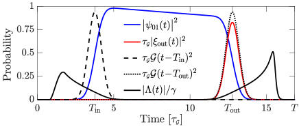
Figure 4: Plots of the solution to Eq. (29) along with the input/output Gaussians and the control field found in Eqs. (37a) and (41a). Parameters: $\gamma\!=\!30\Omega_{\scriptscriptstyle\mathcal{G}}$, $\gamma_{L}\!=\!5\!\times\!10^{-3}\Omega_{\scriptscriptstyle\mathcal{G}}$, $\tau_{\rm{e}}\!=\!\tau_{\!\scriptscriptstyle\mathcal{G}}$, $\tau_{o}\!=\!4.08\tau_{\!\scriptscriptstyle\mathcal{G}}$, $T_{\rm{store}}\!=\!9\tau_{\!\scriptscriptstyle\mathcal{G}}$.

The control field is given by $\Lambda\!=\!\Lambda_{i}\!+\!\Lambda_{o}$ since the storage time, $T_{\rm{store}}$, is chosen large enough to avoid overlap between the absorption and emission intervals, $T_{\rm{store}}\!>\!T_{\rm{in}}\!+\!\tau_{o}$. Note that the control field responsible for emission is different from a simple time-inversion of the control field responsible for absorption. This is because the presence of loss breaks the time-reversal symmetry of the equations of motion in Eq. (29).

In the presence of loss, it is possible to emit a wave packet with the desired shape but reduced amplitude, $\xi_{\rm{out}}(t)\!\approx\!\sqrt{\eta}\mathcal{G}(t-T_{\rm{out}})$, where $\eta$ is a real number smaller than 1. Note, however, that this is only true in the emission interval, $t\!\in\![T_{\rm{out}}\!-\!\tau_{o},T]$, since $\xi_{\rm{out}}(t)$ generally has some small contribution from the absorption interval due to imperfect absorption. The probability that the photon passes by the cavity without being absorbed is

$$P_{\rm{pass}}\equiv\int_{0}^{2T_{\rm{in}}}\!|\xi_{\rm{out}}(t)|^{2}dt.$$ (46)

The probability of a successful storage process is equal to $\eta$ in the limit $P_{\rm{pass}}\rightarrow 0$. The maximum possible value of $\eta$ can be found by inserting $\xi\!=\!\sqrt{\eta}\mathcal{G}$ into the denominator of Eq. (41a) and ensuring that the terms under the square root are positive for all $t$. For the Gaussian in Eq. (44), we have

$$\mathcal{F}_{o}\equiv 2\!\int_{-\infty}^{\infty}\!\!\!f_{o}(t)dt=\gamma\exp\!\Big{[}\gamma_{L}\Big{(}T_{\rm{out}}\!+\!\frac{\gamma_{L}\tau_{\!\scriptscriptstyle\mathcal{G}}^{2}}{16\ln(2)}\Big{)}\Big{]},$$ (47)

and we therefore choose $\eta$ as

$$\eta=\frac{\gamma|\psi_{01}(0)|^{2}}{\mathcal{F}_{o}}\big{(}1-\epsilon_{\eta}\big{)}.$$ (48)

The value of the small parameter, $\epsilon_{\eta}$, is optimized to maximize the value of $\eta$ while avoiding divergences in $|\Lambda_{o}|$. Finite values of $P_{\rm{pass}}$ limits the achievable overlap of the output wave packet with a desired shape, which is seen by calculating the conditional fidelity in Eq. (25) using $\xi_{\rm{out}}\!=\!\sqrt{\eta}\mathcal{G}(t\!-\!T_{\rm{out}})$ in the emission interval

$$\overline{F}_{1}=\frac{\Big{|}\int_{0}^{T}\!\xi_{\rm{out}}(t)\mathcal{G}(t\!-\!T_{\rm{out}})^{*}dt\Big{|}^{2}}{\int_{0}^{T}\!|\xi_{\rm{out}}(t)|^{2}dt}\approx\frac{\eta}{P_{\!\rm{pass}}\!+\!\eta},$$ (49)

where we changed the lower integration limit from 0 to $T_{\rm{out}}\!-\!\tau_{\rm{o}}$ in the numerator since $\mathcal{G}(t\!-\!T_{\rm{out}})\!\approx\!0$ outside the emission interval. We also divided the integration of $|\xi_{\rm{out}}|^{2}$ into intervals $[0,2T_{\rm{in}}]$ and $[T_{\rm{out}}\!-\!\tau_{\rm{o}},T]$ since $|\xi_{\rm{out}}(t)|^{2}\!\approx\!0$ in the storage interval.

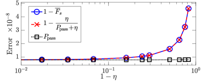
Figure 5: Degradation of conditional fidelity in the limit of large loss. Parameters: $\gamma\!=\!30\Omega_{\scriptscriptstyle\mathcal{G}}$, $\tau_{\rm{e}}\!=\!\tau_{\!\scriptscriptstyle\mathcal{G}}$.

Fig. 5 shows a plot of the conditional fidelity using $\xi_{\rm{out}}$ from Eq. (29) along with the approximation in Eq. (49). It also shows that $\overline{F}_{\!s}\!\rightarrow\!1-P_{\!\rm{pass}}$ in the limit where $P_{\!\rm{pass}}\!\ll\!\eta$, which is seen from a Taylor expansion of Eq. (49), $\overline{F}_{\!s}\approx 1/(1+P_{\!\rm{pass}}/\eta)\approx 1-P_{\!\rm{pass}}$. It is important to note that Fig. 5 clearly illustrates that very small error in the conditional fidelity is possible even in the case of an efficiency well below unity.

The value of $P_{\rm{pass}}$ only depends on the ratio $\gamma/\Omega_{\scriptscriptstyle\mathcal{G}}$ and Fig. 6 plots the dependence for both second- and third-order nonlinear materials.

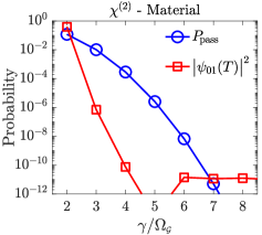
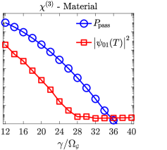
Figure 6: $P_{\rm{pass}}$ as a function of $\gamma/\Omega_{\scriptscriptstyle\mathcal{G}}$ for $\chi^{(2)}$ and $\chi^{(3)}$ materials. Parameters: $\gamma_{L}\!=\!0$, $\tau_{\rm{e}}\!=\!\tau_{\!\scriptscriptstyle\mathcal{G}}$.

It is seen that $P_{\rm{pass}}$ falls off faster for $\chi^{(2)}$ materials due to the absence of cross-phase modulation. In Appendix E.1 we derive expressions suggesting that a five times larger coupling rate, $\gamma$, is needed for a $\chi^{(3)}$ material, which agrees well with the result in Fig. 6. Importantly, Fig. 6 shows that $P_{\rm{pass}}$ approaches zero extremely fast as the ratio $\gamma/\Omega_{\scriptscriptstyle\mathcal{G}}$ increases.

VI Nonlinear Dynamics

In this section we consider three types of nonlinearities that mediate photon-photon interactions and describe the necessary extensions to the equations of motion in Section IV to account for them. Since we have a particular interest in two-qubit logic gates for quantum information processing, we consider cavity configurations enabling a c-phase gate. Note that we envision a configuration where two identical cavities are placed in between two 50/50 beam-splitters that convert the two-qubit state $|{11}\rangle$ into $1/\sqrt{2}(|{02}\rangle+|{20}\rangle)$ [21, 22]. In this case, the phase $\theta_{n}$ in Eq. (20) is important in that $\theta_{2}\!-\!2\theta_{1}\!=\!\pi$ is required for the gate transformation $|{00}\rangle\rightarrow|{00}\rangle$, $|{10}\rangle\rightarrow|{10}\rangle$, $|{01}\rangle\rightarrow|{01}\rangle$, $|{11}\rangle\rightarrow-|{11}\rangle$.

We start by considering a material with a third-order nonlinearity, then we describe second-order nonlinearities, and finally interactions with a two-level emitter.

VI.1 Material with a Third-order Nonlinearity

Only modes $a$ and $b$ are needed in the case of a $\chi^{\scriptscriptstyle(3)}$ material. The Hamiltonian corresponding to photon-photon interactions is

$$\hat{H}_{\!\chi^{(3)}}\!=\!\hbar\chi_{3}\Big{[}\hat{a}^{\dagger}\hat{a}\hat{b}^{\dagger}\hat{b}+\frac{\big{(}\hat{a}^{\dagger}\hat{a}\!-\!1\big{)}\hat{a}^{\dagger}\hat{a}+\big{(}\hat{b}^{\dagger}\hat{b}\!-\!1\big{)}\hat{b}^{\dagger}\hat{b}}{4}\Big{]}.$$ (50)

The corresponding unitary time-evolution operator is

$$\hat{U}_{\!\chi^{(3)}}=-i\Delta t\chi_{3}\hat{b}^{\dagger}\hat{b}\hat{a}^{\dagger}\hat{a}~{}-\\ i\frac{1}{4}\Delta t\chi_{3}\Big{[}\big{(}\hat{b}^{\dagger}\hat{b}-1\big{)}\hat{b}^{\dagger}\hat{b}+\big{(}\hat{a}^{\dagger}\hat{a}-1\big{)}\hat{a}^{\dagger}\hat{a}\Big{]}\!.$$ (51)

Only states with two photons in the system are affected, so that

$$\hat{U}_{\!\chi^{(3)}}|{20}\rangle =-i\chi_{3}\Delta t\frac{1}{4}\big{(}2-1\big{)}2|{20}\rangle=-i\frac{\chi_{3}}{2}\Delta t|{20}\rangle$$ (52a)

$$\hat{U}_{\!\chi^{(3)}}|{11}\rangle =-i\chi_{3}\Delta t|{11}\rangle$$ (52b)

$$\hat{U}_{\!\chi^{(3)}}|{02}\rangle =-i\chi_{3}\Delta t\frac{1}{4}\big{(}2-1\big{)}2|{02}\rangle=-i\frac{\chi_{3}}{2}\Delta t|{02}\rangle.$$ (52c)

The equations of motion for the corresponding coefficients in Eq. (33) are therefore modified as

$$\!\dot{\psi}_{20} \!=-\Big{(}i2\delta_{a}+\Gamma\!+\!i\frac{\chi_{3}}{2}\!+\!i4|\Lambda|\Big{)}\psi_{20}\!-\!i\sqrt{2}\Lambda^{\!*}\psi_{11}~{}+$$

$$\hskip 150.79968pt\sqrt{2\gamma}\psi_{10}^{\rm{ii}}\xi_{\rm{in}}$$ (53a)

$$\!\dot{\psi}_{11} \!=-\Big{(}i(\delta_{a}+\delta_{b})+\frac{\Gamma+\gamma_{L}}{2}+i\chi_{3}+i4|\Lambda|\Big{)}\psi_{11}~{}-$$

$$\hskip 62.59596pti\sqrt{2}\Big{[}\Lambda\psi_{20}\!+\!\Lambda^{\!*}\psi_{02}\Big{]}\!+\!\sqrt{\gamma}\psi_{01}^{\rm{ii}}\xi_{\rm{in}}$$ (53b)

$$\!\dot{\psi}_{02} \!=\!-\Big{(}i2\delta_{b}\!+\!\gamma_{L}\!+\!i\frac{\chi_{3}}{2}\!+\!i4|\Lambda|\Big{)}\psi_{02}-i\sqrt{2}\Lambda\psi_{11}.$$ (53c)

It is seen from Eq. (53c) that the amplitude of the state $|{02}\rangle$ acquires a phase proportional to $\chi_{3}/2$, which the amplitude of the state $|{01}\rangle$ in Eq. (29b) does not. By a careful choice of storage time, $T_{\rm{store}}$, one may achieve the condition $\Delta\theta\!=\!\theta_{2}-2\theta_{1}\!=\!\pi$, where $\theta_{n}$ is the phase in Eq. (20). Fig. 7 plots the phase difference as a function of storage time for a range of different nonlinear coupling coefficients, $\chi_{3}$.

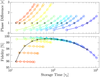
Figure 7: Nonlinear phase difference, $\Delta\theta$, and fidelity, $F_{2}$, as a function of storage time for different values of the nonlinear coupling rate, $\chi_{3}$, ranging from $0.01\Omega_{\scriptscriptstyle\mathcal{G}}$ (blue) to $0.5\Omega_{\scriptscriptstyle\mathcal{G}}$ (red). The black line shows the fidelity corresponding to $\Delta\theta\!=\!\pi$. Parameters: $\gamma\!=\!30\Omega_{\scriptscriptstyle\mathcal{G}}$, $\gamma_{L}\!=\!10^{-5}\Omega_{\scriptscriptstyle\mathcal{G}}$, $\tau_{\rm{e}}\!=\!\tau_{\!\scriptscriptstyle\mathcal{G}}$.

It shows how the phase condition, $\Delta\theta\!=\!\pi$, may be met using a smaller nonlinearity and larger storage time (blue curve) or a larger nonlinearity and smaller storage time (red curve). Fig. 7 also plots the corresponding fidelity, $F_{2}$, which appears to reach an optimum for $T_{\rm{store}}\approx 100\tau_{\!\scriptscriptstyle\mathcal{G}}$. The fidelity degrades when increasing $\chi_{3}$ because the solutions for the control fields were found assuming a single photon input and photon-photon interactions during the absorption and emission process renders the control fields sub-optimal. The fidelity also degrades if $\chi_{3}$ is decreased too much because losses increase with increased storage time.

VI.2 Material with a Second-order Nonlinearity

For materials exhibiting a $\chi^{\scriptscriptstyle(2)}$ nonlinearity, we explore the process of second-harmonic-generation where $\omega_{c}\!=\!2\omega_{b}$. With the introduction of mode $c$, the system states are written as $|{n_{a}n_{b}n_{c}}\rangle\equiv|{n_{a}}\rangle|{n_{b}}\rangle|{n_{c}}\rangle$ with $n_{a},~{}n_{b}$, and $n_{c}$ representing the number of photons in each mode. The Hamiltonian describing the interaction is given in Eq. (13b). The corresponding unitary time-evolution operator is

$$\hat{U}_{\rm{SHG}}=-i\chi_{2}\Delta t\Big{(}\hat{c}\hat{b}^{\dagger}\hat{b}^{\dagger}+\hat{c}^{\dagger}\hat{b}\hat{b}\Big{)}.$$ (54)

From Eq. (54) we see that it only causes a coupling between states $|{020}\rangle$ and $|{001}\rangle$

$$\hat{U}_{\rm{SHG}}|{020}\rangle =-i\chi_{2}\Delta t\sqrt{2}|{001}\rangle$$ (55a)

$$\hat{U}_{\rm{SHG}}|{001}\rangle =-i\chi_{2}\Delta t\sqrt{2}|{020}\rangle.$$ (55b)

The equations of motion for coefficients corresponding to two photons in the system are then

$$\dot{\psi}_{200} =\!-\!\big{(}i2\delta_{a}\!+\!\Gamma\big{)}\psi_{200}\!-\!i\sqrt{2}\Lambda^{\!*}\psi_{110}\!+\!\sqrt{2\gamma}\psi_{100}^{\rm{ii}}\xi_{\rm{in}}$$ (56a)

$$\dot{\psi}_{110} =-\Big{(}i(\delta_{a}\!+\!\delta_{b})\!+\!\frac{\Gamma+\gamma_{L}}{2}\Big{)}\psi_{110}-i\sqrt{2}\Lambda\psi_{200}~{}-$$

$$\hskip 85.35826pti\sqrt{2}\Lambda^{\!*}\psi_{020}+\sqrt{\gamma}\psi_{01}^{\rm{ii}}\xi_{\rm{in}}$$ (56b)

$$\dot{\psi}_{020} =-\big{(}i2\delta_{b}\!+\!\gamma_{L}\big{)}\psi_{020}\!-\!i\sqrt{2}\Lambda\psi_{110}\!-\!i\sqrt{2}\chi_{2}\psi_{001}$$ (56c)

$$\dot{\psi}_{001} =-\Big{(}i\delta_{c}+\frac{\gamma_{L}}{2}\Big{)}\psi_{001}-i\sqrt{2}\chi_{2}\psi_{020}.$$ (56d)

It is the fact that SHG requires two input photons that enables the phase condition $\Delta\theta\!=\!\pi$ to be fulfilled. To understand why, consider the case in which the storage time is adjusted such that a single Rabi-flip between states $|{020}\rangle$ and $|{001}\rangle$ occur. An example is shown in Fig. 8. Occupation probabilities of the system states are found in Appendix D and plotted as a function of time in Fig. 8a. It shows how the photons are transferred from state $|{020}\rangle$ to $|{001}\rangle$ and back via SHG. The phase of $\psi_{020}(t)$ jumps by $\pi$ as its amplitude becomes zero in the middle of the storage interval (red curve in Fig. 8b).

Figure 8: (a) Occupation probabilities of system states as a function of time. (b) Phase of the coefficient corresponding to state $|{01}\rangle$ (blue) and $|{020}\rangle$ (red). (c) Error measured as the absolute distance from a Gaussian, $|\xi_{\rm{out}}(t)\!-\!\sqrt{\eta}\mathcal{G}(t\!-\!T_{\rm{out}})|$ (blue) and $|\xi_{\rm{out}}(\tau,T_{\rm{out}})\!+\!\eta\mathcal{G}(\tau\!-\!T_{\rm{out}})\mathcal{G}(0)|$ (red). Parameters: $\gamma\!=\!6\Omega_{\scriptscriptstyle\mathcal{G}}$, $\gamma_{L}\!=\!1.5\!\times\!10^{-4}\Omega_{\scriptscriptstyle\mathcal{G}}$, $\tau_{\rm{e}}\!=\!\tau_{\!\scriptscriptstyle\mathcal{G}}$, $\eta\!=\!0.9963$.

The phase of $\psi_{01}(t)$ (blue curve in Fig. 8b) remains constant since a single photon cannot undergo SHG. The relevant phase difference, $\Delta\theta$, is therefore seen to be exactly $\pi$. Fig. 8c shows the error in the output wave packet for both single- and two-photon inputs. Only a negligible error is observed for the single-photon input whereas the two-photon error is more pronounced leading to a fidelity of $F_{2}\!=\!99.1\%$ for this example. Similar to the case of a $\chi^{(3)}$ material, the fidelity of two-photon outputs are degraded by the photon-photon interaction occurring during the absorption and emission process, which is not accounted for in the solution of the control fields.

VI.3 Interaction with a Two-Level Emitter

We investigate the use of atom-like two-level emitters because their nonlinearity is much stronger than the non-resonant nonlinearities considered above. To ensure complete absorption of incoming photons, the TLE should not be coupled to mode $b$ since we expect the nonlinear interaction during absorption and emission to be prohibitively strong. Instead, we use a tertiary mode, $c$, such that $\omega_{c}\!-\!\omega_{b}\sim\omega_{b}\!-\!\omega_{a}$ is in the GHz range. We envision a control scheme where a first control pulse, $\Lambda_{i}(t)$, is used to absorb incoming photons into mode $b$. Subsequently, a second control pulse, $\Pi(t)$, couples modes $b$ and $c$. Finally, a third control pulse, $\Lambda_{o}(t)$, couples the photons back into the waveguide through mode $a$. The first and last stage of this control protocol is therefore still described by the equations of motion in Section IV.4. With the introduction of cavity mode $c$ and the TLE, states with two photons in the system are: $|{100}\rangle|{e}\rangle$, $|{010}\rangle|{e}\rangle$, $|{001}\rangle|{e}\rangle$, $|{200}\rangle|{g}\rangle$, $|{020}\rangle|{g}\rangle$, $|{002}\rangle|{g}\rangle$, $|{110}\rangle|{g}\rangle$, $|{101}\rangle|{g}\rangle$, and $|{011}\rangle|{g}\rangle$.

During the second stage of the protocol, mode $a$ is empty so we introduce new coefficients, $\phi_{n_{b}n_{c}g}(t)$ and $\phi_{n_{b}n_{c}e}(t)$, corresponding to states $|{0n_{b}n_{c}}\rangle|{g}\rangle$ and $|{0n_{b}n_{c}}\rangle|{e}\rangle$. The dynamics is governed by the following equations of motion

$$\dot{\phi}_{20g} =\!-\!\big{(}i2\delta_{b}\!+\!\gamma_{L}\!+\!i\chi_{3}\!+\!i4|\Pi|\big{)}\phi_{20g}\!-\!i\sqrt{2}\Pi^{*}\phi_{11g}$$ (57a)

$$\dot{\phi}_{11g} =-\big{[}i(\delta_{b}+\delta_{c})+\gamma_{L}+i\chi_{3}+i4|\Pi|\big{]}\phi_{11g}~{}-$$

$$\hskip 51.21504pti\sqrt{2}\Pi\phi_{20g}-i\sqrt{2}\Pi^{*}\phi_{02g}-ig\phi_{10e}$$ (57b)

$$\dot{\phi}_{02g} =-\big{(}i2\delta_{c}+\gamma_{L}+i\chi_{3}+i4|\Pi|\big{)}\phi_{02g}~{}-$$

$$\hskip 96.73918pti\sqrt{2}\Pi\phi_{11g}-i\sqrt{2}g\phi_{01e}$$ (57c)

$$\dot{\phi}_{10e} =-\Big{(}i(\delta_{b}\!+\!\delta_{e})+\frac{\gamma_{e}+\gamma_{L}}{2}+i2|\Pi|\Big{)}\phi_{10e}~{}-$$

$$\hskip 113.81102pti\Pi^{*}\phi_{01e}-ig^{*}\phi_{11g}$$ (57d)

$$\dot{\phi}_{01e} =-\Big{(}i(\delta_{c}\!+\!\delta_{e})+\frac{\gamma_{e}+\gamma_{L}}{2}+i2|\Pi|\Big{)}\phi_{01e}~{}-$$

$$\hskip 105.2751pti\Pi\phi_{10e}-i\sqrt{2}g^{*}\phi_{02g}.$$ (57e)

Note that the dynamics is also changed for single-photon inputs, which have the following equations of motion

$$\dot{\phi}_{10g} =-\Big{(}i\delta_{b}+\frac{\gamma_{L}}{2}+i2|\Pi|\Big{)}\phi_{10g}-i\Pi^{*}\phi_{01g}$$ (58a)

$$\dot{\phi}_{01g} =-\Big{(}i\delta_{c}\!+\!\frac{\gamma_{L}}{2}\!+\!i2|\Pi|\Big{)}\phi_{01g}\!-\!i\Pi\phi_{10g}\!-\!ig\phi_{00e}$$ (58b)

$$\dot{\phi}_{00e} =-\Big{(}i\delta_{e}+\frac{\gamma_{e}}{2}\Big{)}\phi_{00e}-ig^{*}\phi_{01g}.$$ (58c)

Many interesting properties of the nonlinear interaction may be investigated using Eqs. (57) and (58) but here we again consider the implementation of a c-phase gate. With the protocol described above, the conditions for a successful gate operation are: 1) The occupation probability of mode $b$ must equal one for both single- and two-photon inputs after the application of $\Pi(t)$. 2) The phase difference must be $\arg[\phi_{20g}(T_{\Pi})]\!-\!2\arg[\phi_{10g}(T_{\Pi})]\!=\!\pi$, where $\Pi(t)$ is non-zero only in the interval $t\!\in\![2T_{\rm{in}},T_{\Pi}]$. We numerically optimize the control function $\Pi(t)$ to fulfill these conditions.

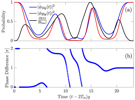
Figure 9: Time evolution of the second stage of the control protocol. (a) Probability that all incoming photons occupy mode $b$ for one- (blue) and two-photon (red) inputs. The control function is also plotted (scaled to a maximum of 1). (b) Phase difference $\arg[\phi_{20g}(t\!-\!2T_{\rm{in}})]\!-\!2\arg[\phi_{10g}(t\!-\!2T_{\rm{in}})]$ as a function of time. Parameters: $\gamma_{L}\!=\!0$.

An example of the resulting dynamics is shown in Fig. 9. It shows how the conditions above may be met using a control function plotted in Fig. 9a.

Here, we considered the host crystal containing the TLE to be a third-order nonlinear material. Many types of TLEs are sensitive to electric fields, which could become problematic if the control field originated from and applied RF field. The optical control fields would not interact with the TLE as they would be very far off-resonant. However, it would be interesting to consider the TLE coupled to mode $b$ and whether an RF control field, $\Lambda(t)$, would be strong enough to effectively detune the TLE and mode $b$ during absorption and emission via an AC Stark shift of the TLE transition energy. This would reduce the effective nonlinear coupling between the photons during absorption and emission and could potentially eliminate the need for mode $c$ and increase the gate operation speed.

An alternative protocol would still use optical control fields for $\Lambda(t)$, to load the photons into mode $b$. The TLE would be coupled to mode $b$, but its transition energy, $\omega_{e}(t)$, would be controllable via an electrical control field that again tunes the TLE in- and out of resonance with mode $b$ via the AC Stark shifts. During the absorption and emission, the detuning would be large to eliminate any nonlinear interaction, while a similar numerical optimization technique could be used to determine the temporal shape of the electrical control field to implement the c-phase gate.

Note that the three-stage control protocol avoids any error due to nonlinear interactions between the photons during absorption and emission. The fidelity of a c-phase gate with a TLE nonlinearity is therefore only limited by loss when no decoherence mechanisms are included in the model. A similar extension of the control protocol could be applied to the case of second-order nonlinearities by introducing a fourth mode, $b^{\prime}$, coupled to mode $c$ via SHG. A second control field, $\Pi(t)$, coupling modes $b$ and $b^{\prime}$ would then effectively turn on the nonlinearity after the photons were coupled into mode $b$.

VII Discussion

Our simulation results illustrate that, within the limitations of our model, it is possible to absorb and emit photons with Gaussian wave packets into- and out of a dynamically coupled cavity. We also show that high fidelity c-phase gates may be implemented using such structures with three different types of nonlinearity. These fidelities were obtained while excluding certain sources of error from our analysis including noise-photons being injected from the loss channel at finite temperatures and decoherence of the TLE.

We analyzed the interaction with two-level emitters in the context of two-qubit gates, but we expect dynamically coupled cavities to provide performance improvements in other applications as well. For instance, perfect state transfer between photonic qubits and solid-state matter qubits has been proposed using classical control fields coupling the energy levels of the matter qubit [23]. There is a strong analogy between that method and dynamically coupled cavities, however, we expect it to be easier to engineer the photonic- rather than the atomic degrees of freedom in practical implementations.

Appendix A Rotating Frame

The Hamiltonian of the three cavity modes, four pump fields, and the TLE is $\hat{H}$, where

$$\frac{\hat{H}}{\hbar}=\omega_{a}\hat{a}^{\dagger}\hat{a}+\omega_{b}\hat{b}^{\dagger}\hat{b}+\omega_{c}\hat{c}^{\dagger}\hat{c}+\omega_{p}\hat{p}^{\dagger}\hat{p}+\omega_{1}\hat{p}_{1}^{\dagger}\hat{p}_{1}+\omega_{2}\hat{p}_{2}^{\dagger}\hat{p}_{2}+\omega_{3}\hat{p}_{3}^{\dagger}\hat{p}_{3}+\omega_{e}\hat{\sigma}_{z}+i\sqrt{\frac{\gamma}{\Delta t}}\Big{(}\hat{a}^{\dagger}\hat{w}_{n}-\hat{a}\hat{w}_{n}^{\dagger}\Big{)}~{}+\\ \omega_{w}\!\sum_{k=1}^{N}\hat{w}_{k}^{\dagger}\hat{w}_{k}+\chi_{2}\Big{(}\hat{p}^{\dagger}\hat{a}^{\dagger}\hat{b}+\hat{p}\hat{b}^{\dagger}\hat{a}\Big{)}+\chi_{3}\Big{(}\hat{p}_{1}^{\dagger}\hat{p}_{2}\hat{a}^{\dagger}\hat{b}+\hat{p}_{2}^{\dagger}\hat{p}_{1}\hat{b}^{\dagger}\hat{a}\Big{)}+\chi_{3}\Big{(}\hat{p}_{1}^{\dagger}\hat{p}_{3}\hat{b}^{\dagger}\hat{c}+\hat{p}_{3}^{\dagger}\hat{p}_{1}\hat{c}^{\dagger}\hat{b}\Big{)}.$$ (59)

(Since we wish merely to provide an example, we have left out the cross-phase modulation, self-phase modulation, and second harmonic generation from the Hamiltonian.) We wish to move into the interaction picture, placing the evolution generated by the Hamiltonian $H_{0}$ into the operators, where

$$\frac{H_{0}}{\hbar}=\omega_{w}\hat{a}^{\dagger}\hat{a}+(\omega_{b}\!-\!\delta_{b})\hat{b}^{\dagger}\hat{b}+(\omega_{c}\!-\!\delta_{c})\hat{c}^{\dagger}\hat{c}+\omega_{c}\hat{\sigma}_{z}+\omega_{p}\hat{p}^{\dagger}\hat{p}+\omega_{1}\hat{p}_{1}^{\dagger}\hat{p}_{1}+\omega_{2}\hat{p}_{2}^{\dagger}\hat{p}_{2}+\omega_{3}\hat{p}_{3}^{\dagger}\hat{p}_{3}+\omega_{w}\!\sum_{k=1}^{N}\hat{w}_{k}^{\dagger}\hat{w}_{k}.$$ (60)

Under this Hamiltonian the evolution of the operators is obtained merely by multiplying them by time-dependent exponentials. Denoting the interaction-picture operators by upper-case letters, we have $\hat{A}=\hat{a}e^{-i\omega_{w}t}$, $\hat{B}=\hat{b}e^{-i(\omega_{b}\!-\!\delta_{b})t}$, $\hat{C}=\hat{c}e^{-i(\omega_{c}\!-\!\delta_{c})t}$, $\hat{\Sigma}_{z}=\hat{\sigma}_{z}e^{-i\omega_{e}t}$, $\hat{P}=\hat{p}e^{-i\omega_{p}t}$, $\hat{P}_{j}=\hat{p}_{j}e^{-i\omega_{j}t}$ ($j=1,2,3$), $\hat{W}_{k}=\hat{w}_{k}e^{-i\omega_{w}t_{k}}$. Since we have removed this “rotating” evolution from the state of the system, we refer to the interaction picture as being in a “rotating frame”.

The evolution of the state of the system is now given by an effective interaction Hamiltonian, usually referred to as the “interaction Hamiltonian in the interaction picture”, which is given by

$$\hat{H}_{\rm{I}}(t)=\hat{U}(\hat{H}-\hat{H}_{0})\hat{U}^{\dagger}$$ (61)

in which $\hat{U}=e^{-i\hat{H}_{0}t/\hbar}$. Since the right-hand side of the above equation is merely the Hamiltonian $\hat{H}-\hat{H_{0}}$ evolved in the interaction picture, we obtain $\hat{H}_{\rm{I}}(t)$ merely by replacing the Schrödinger picture operators in $\hat{H}-\hat{H_{0}}$ with their interaction picture counterparts given above. While in general $\hat{H}_{\rm{I}}(t)$ will be time-dependent, if we choose the detuning parameters, $\delta_{a}$ through $\delta_{e}$, to account for the detunings between the various modes and the TLE, we obtain a time-independent interaction picture Hamiltonian, namely

$$\hat{H}_{\rm{rot}}=\hbar\delta_{a}\hat{a}^{\dagger}\hat{a}+\hbar\delta_{b}\hat{b}^{\dagger}\hat{b}+\hbar\delta_{c}\hat{c}^{\dagger}\hat{c}+\hbar\delta_{e}\hat{\sigma}_{z}+i\hbar\sqrt{\frac{\gamma}{\Delta t}}\Big{(}\hat{a}^{\dagger}\hat{w}_{n}-\hat{a}\hat{w}_{n}^{\dagger}\Big{)}+\hbar\chi_{2}\Big{(}\hat{p}^{\dagger}\hat{a}^{\dagger}\hat{b}+\hat{p}\hat{b}^{\dagger}\hat{a}\Big{)}~{}+\\ \hbar\chi_{3}\Big{(}\hat{p}_{1}^{\dagger}\hat{p}_{2}\hat{a}^{\dagger}\hat{b}+\hat{p}_{2}^{\dagger}\hat{p}_{1}\hat{b}^{\dagger}\hat{a}\Big{)}+\hbar\chi_{3}\Big{(}\hat{p}_{1}^{\dagger}\hat{p}_{3}\hat{b}^{\dagger}\hat{c}+\hat{p}_{3}^{\dagger}\hat{p}_{1}\hat{c}^{\dagger}\hat{b}\Big{)}.$$ (62)

For the scenario in which the non-linearity is provided by the TLE, the various detunings are chosen to satisfy

$$\left.\begin{array}[]{rcl}\qquad\delta_{a}&\equiv&\omega_{a}-\omega_{w}\\ \delta_{b}&\equiv&\delta_{\Lambda}+\delta_{a}\\ \delta_{c}&\equiv&\delta_{\Pi}+\delta_{b}\\ \delta_{e}&\equiv&\omega_{e}-\omega_{c}\\ \delta_{\Lambda}&\equiv&(\omega_{2}-\omega_{1})-(\omega_{a}-\omega_{b})\\ \delta_{\Pi}&\equiv&(\omega_{3}-\omega_{1})-(\omega_{b}-\omega_{c})\end{array}\right\}\;\;\;\mbox{TLE nonlinearity .}$$ (69)

Here we have chosen $\delta_{b}$ to remove the oscillating exponential factor in the FWM term corresponding to the control field $\Lambda(t)$:

$$\hat{P}_{2}^{\dagger}\hat{P}_{1}\hat{B}^{\dagger}\hat{A} =\hat{p}_{2}^{\dagger}\hat{p}_{1}\hat{b}^{\dagger}\hat{a}\exp\big{[}(\omega_{2}-\omega_{1})+\omega_{b}-\delta_{b}-(\omega_{a}-\delta_{a})\big{]}~{}\Rightarrow$$

$$\delta_{b} =(\omega_{2}-\omega_{1})-(\omega_{a}-\omega_{b})+\delta_{a}\equiv\delta_{\Lambda}+\delta_{a},$$ (70)

where we have defined $\delta_{\Lambda}$, which describes energy mismatch in the FWM process that couples modes $a$ and $b$. Similarly, we choose $\delta_{c}$ to remove any exponential factor on the FWM term corresponding to the control field $\Pi(t)$

$$\hat{P}_{3}^{\dagger}\hat{P}_{1}\hat{C}^{\dagger}\hat{B} =\hat{p}_{3}^{\dagger}\hat{p}_{1}\hat{c}^{\dagger}\hat{b}\exp\big{[}(\omega_{3}-\omega_{1})-(\omega_{b}-\delta_{b})+(\omega_{c}-\delta_{c})\big{]}~{}\Rightarrow$$

$$\delta_{c} =(\omega_{3}-\omega_{1})-(\omega_{b}-\omega_{c})+\delta_{b}\equiv\delta_{\Pi}+\delta_{b},$$ (71)

where we defined $\delta_{\Pi}$, which describes energy mismatch in the FWM process that couples modes $b$ and $c$.

In a $\chi^{(2)}$ material, where there is no control field $\Pi(t)$, we instead define the detunings as

$$\left.\begin{array}[]{rcl}\delta_{a}&\equiv&\omega_{a}-\omega_{w}\\ \delta_{b}&\equiv&\delta_{\Lambda}+\delta_{a}\\ \delta_{c}&\equiv&\omega_{c}-2\omega_{b}\\ \delta_{\Lambda}&\equiv&\omega_{p}-(\omega_{b}-\omega_{a})\end{array}\right\}\;\;\;\mbox{$\chi^{(2)}$ material},$$ (76)

where $\delta_{c}$ now describes energy mismatch in the second harmonic generation process.

Appendix B Dynamics with One Cavity Mode and One Input Photon

Before the dynamics begins, the state is

$$|{\psi_{0}}\rangle=\sum_{k=1}^{N}\xi^{\rm{in}}_{k}\sqrt{\Delta t}|{0}\rangle|{1_{k}}\rangle,$$ (77)

where $|{0}\rangle|{1_{k}}\rangle$ is the state with one photon in bin $k$ and no photons in the system. The state after each time step is found using the time evolution operator

$$|{\psi_{n+1}}\rangle=\hat{U}_{n+1}|{\psi_{n}}\rangle.$$ (78)

After the first time step, the state is therefore

$$|{\psi_{1}}\rangle=\sum_{k=1}^{N}\xi^{\rm{in}}_{k}\sqrt{\Delta t}|{0}\rangle|{1_{k}}\rangle+\sqrt{\gamma}\xi^{\rm{in}}_{1}\Delta t|{1}\rangle|{\emptyset}\rangle\equiv\sum_{k=1}^{N}\xi^{\rm{in}}_{k}\sqrt{\Delta t}|{0}\rangle|{1_{k}}\rangle+\psi_{1}(1)|{1}\rangle|{\emptyset}\rangle,$$ (79)

where the second term correspond to a photon in bin 1 being absorbed into the cavity mode. After the second step, the state is

$$|{\psi_{2}}\rangle=\sum_{k=1}^{N}\xi^{\rm{in}}_{k}\sqrt{\Delta t}|{0}\rangle|{1_{k}}\rangle-\sqrt{\gamma}\psi_{1}(1)\sqrt{\Delta t}|{0}\rangle|{\mathbf{1}_{2}}\rangle+\Big{[}\Big{(}1-i\delta_{a}\Delta t-\frac{\Gamma}{2}\Delta t\Big{)}\psi_{1}(1)+\sqrt{\gamma}\xi^{\rm{in}}_{2}\Delta t\Big{]}|{1}\rangle|{\emptyset}\rangle,$$ (80)

where the second term corresponds to a photon being emitted by the cavity into bin 2 on the output side (note that we use boldface notation to distinguish input from output photons). The third term contains a contribution from the identity operator, a decay term, as well as a feeding term corresponding to absorption of a photon from the waveguide in bin 2. At this point, we split the sum over $k$ into $k>n$ corresponding to the photon being on the input side (see Fig. 2) and $k\leq n$ corresponding to the photon being on the output side

$$|{\psi_{2}}\rangle=\sum_{k=3}^{N}\xi^{\rm{in}}_{k}\sqrt{\Delta t}|{0}\rangle|{1_{k}}\rangle+\xi^{\rm{out}}_{1}\sqrt{\Delta t}|{0}\rangle|{\mathbf{1}_{1}}\rangle+\Big{[}\xi^{\rm{in}}_{2}-\sqrt{\gamma}\psi_{1}(1)\Big{]}\sqrt{\Delta t}|{0}\rangle|{\mathbf{1}_{2}}\rangle+\psi_{1}(2)|{1}\rangle|{\emptyset}\rangle.$$ (81)

Eqs. (80) and (81) contain all types of states and we can use them to identify the update rules

$$\psi_{1}(n+1) =\psi_{1}(n)+\Big{[}\Big{(}-i\delta_{a}-\frac{\Gamma}{2}\Big{)}\psi_{1}(n)+\sqrt{\gamma}\xi^{\rm{in}}_{n+1}\Big{]}\Delta t~{}~{}\Rightarrow$$ (82)

$$\frac{\psi_{1}(n+1)-\psi_{1}(n)}{\Delta t} =-\Big{(}i\delta_{a}+\frac{\Gamma}{2}\Big{)}\psi_{1}(n)+\sqrt{\gamma}\xi^{\rm{in}}_{n+1}$$ (83)

$$\xi^{\rm{out}}_{n} =\xi^{\rm{in}}_{n}-\sqrt{\gamma}\psi_{1}(n-1).$$ (84)

We may now take the continuum limit, $\Delta t\rightarrow 0$, to obtain the equation of motion and input-output relation

$$\dot{\psi}_{1}(t) =\Big{(}-i\delta_{a}-\frac{\Gamma}{2}\Big{)}\psi_{1}(t)+\sqrt{\gamma}\xi_{\rm{in}}(t)$$ (85a)

$$\xi_{\rm{out}}(t) =\xi_{\rm{in}}(t)-\sqrt{\gamma}\psi_{1}(t).$$ (85b)

Appendix C Dynamics with Two Cavity Modes and One Input Photon

Before the dynamics begins, the state is

$$|{\psi_{0}}\rangle=\sum_{k=1}^{N}\xi^{\rm{in}}_{k}\sqrt{\Delta t}|{00}\rangle|{1_{k}}\rangle,$$ (86)

where $|{00}\rangle$ is the state with no photons in either mode $a$ or $b$. After step one, the state is

$$|{\psi_{1}}\rangle=|{\psi_{0}}\rangle+\sqrt{\gamma}\xi^{\rm{in}}_{1}\Delta t|{10}\rangle|{\emptyset}\rangle\equiv|{\psi_{0}}\rangle+\psi_{10}(1)|{10}\rangle|{\emptyset}\rangle,$$ (87)

where we defined the amplitude for the state with one photon in mode $a$ and no photons in mode $b$, $\psi_{10}$. After step two, the state is

$$|{\psi_{2}}\rangle=\sum_{k=3}^{N}\xi^{\rm{in}}_{k}\sqrt{\Delta t}|{00}\rangle|{1_{k}}\rangle-\sqrt{\gamma}\psi_{10}(1)\sqrt{\Delta t}|{00}\rangle|{\mathbf{1}_{1}}\rangle+\Big{[}\xi^{\rm{in}}(2)-\sqrt{\gamma}\psi_{10}(1)\Big{]}\sqrt{\Delta t}|{00}\rangle|{\mathbf{1}_{2}}\rangle~{}+\\ \Big{[}\Big{(}1-i\delta_{a}\Delta t-\frac{\Gamma}{2}\Delta t-i2|\Lambda_{2}|\Delta t\Big{)}\psi_{10}(1)+\sqrt{\gamma}\xi^{\rm{in}}_{2}\Big{]}|{10}\rangle|{\emptyset}\rangle-i\Lambda_{2}\psi_{10}(1)\Delta t|{01}\rangle|{\emptyset}\rangle~{}\equiv\\ \sum_{k=3}^{N}\xi^{\rm{in}}_{k}\sqrt{\Delta t}|{00}\rangle|{1_{k}}\rangle+\sum_{k=1}^{2}\xi^{\rm{out}}_{k}\sqrt{\Delta t}|{00}\rangle|{\mathbf{1}_{k}}\rangle+\psi_{10}|{10}\rangle|{\emptyset}\rangle+\psi_{01}|{01}\rangle|{\emptyset}\rangle.$$ (88)

After step three, the state is

$$|{\psi_{3}}\rangle=\sum_{k=4}^{N}\xi^{\rm{in}}_{k}\sqrt{\Delta t}|{00}\rangle|{1_{k}}\rangle\!+\!\sum_{k=1}^{3}\xi^{\rm{out}}_{k}\sqrt{\Delta t}|{00}\rangle|{\mathbf{1}_{k}}\rangle\!+\!\Big{[}\Big{(}1\!-\!i\delta_{b}\Delta t\!-\!\frac{\gamma_{L}}{2}\Delta t\!-\!i2|\Lambda_{3}|\Delta t\Big{)}\psi_{01}(2)\!-\!i\Lambda_{3}\psi_{10}(2)\Delta t\Big{]}|{01}\rangle|{\emptyset}\rangle~{}+\\ \Big{[}\Big{(}1-i\delta_{a}\Delta t-\frac{\Gamma}{2}\Delta t-i2|\Lambda_{3}|\Delta t\Big{)}\psi_{10}(1)-i\Lambda_{3}^{*}\psi_{01}(2)\Delta t+\sqrt{\gamma}\xi^{\rm{in}}_{3}\Big{]}|{10}\rangle|{\emptyset}\rangle.$$ (89)

Eq. (89) contains all the possible dynamics and we can use it to read off the update rules

$$\frac{\psi_{10}(n+1)-\psi_{10}(n)}{\Delta t} =\Big{(}-i\delta_{a}-\frac{\Gamma}{2}-i2|\Lambda_{n+1}|\Big{)}\psi_{10}(n)-i\Lambda_{n+1}^{*}\psi_{01}(n)+\sqrt{\gamma}\xi^{\rm{in}}_{n+1}$$ (90)

$$\frac{\psi_{01}(n+1)-\psi_{01}(n)}{\Delta t} =\Big{(}-i\delta_{b}-\frac{\gamma_{L}}{2}-i2|\Lambda_{n+1}|\Big{)}\psi_{01}(n)-i\Lambda_{n+1}\psi_{10}(n)$$ (91)

$$\xi^{\rm{out}}_{n} =\xi^{\rm{in}}_{n}-\sqrt{\gamma}\psi_{10}(n-1).$$ (92)

In the continuum limit, we have the ODEs and input-output relation

$$\dot{\psi}_{10}(t) =-\Big{(}i\delta_{a}+\frac{\Gamma}{2}+i2|\Lambda(t)|\Big{)}\psi_{10}(n)-i\Lambda(t)^{\!*}\psi_{01}(t)+\sqrt{\gamma}\xi_{\rm{in}}(t)$$ (93a)

$$\dot{\psi}_{01}(t) =-\Big{(}i\delta_{b}+\frac{\gamma_{L}}{2}+i2|\Lambda(t)|\Big{)}\psi_{01}(t)-i\Lambda(t)\psi_{10}(t)$$ (93b)

$$\xi_{\rm{out}}(t) =\xi_{\rm{in}}(t)-\sqrt{\gamma}\psi_{10}(t).$$ (93c)

Appendix D Dynamics with Two Cavity Modes and Two Input Photons

For identical input photons, the input state is

$$|{\psi_{0}}\rangle=\sqrt{2}\sum_{j=1}^{N}\sum_{k>j}^{N}\xi^{\rm{in}}_{j}\xi^{\rm{in}}_{k}\Delta t|{00}\rangle|{1_{j}1_{k}}\rangle.$$ (94)

Let us show that the state in Eq. (94) is normalized. In the continuum limit, it corresponds to

$$|{\psi}\rangle=\sqrt{2}\int_{0}^{T}dt_{j}\int_{t_{j}}^{T}dt_{k}\xi(t_{j})\xi(t_{k})|{00}\rangle|{1_{j}1_{k}}\rangle,$$ (95)

where we omitted the ⁱⁿ superscripts. Let us calculate its norm

$$\big{\langle}{\psi\big{|}\psi}\big{\rangle} =2\int_{0}^{T}dt_{j}^{\prime}\int_{t_{j}^{\prime}}^{T}dt_{k}^{\prime}\int_{0}^{T}dt_{j}\int_{t_{j}}^{T}dt_{k}\xi^{*}(t_{j^{\prime}})\xi(t_{j})\xi^{*}(t_{k^{\prime}})\xi(t_{k})\big{\langle}{1_{j}^{\prime}\big{|}1_{j}}\big{\rangle}\big{\langle}{1_{k}^{\prime}\big{|}1_{k}}\big{\rangle}~{}\Rightarrow$$ (96a)

$$\big{\langle}{\psi\big{|}\psi}\big{\rangle} =2\int_{0}^{T}dt_{j}\big{|}\xi(t_{j})\big{|}^{2}\int_{t_{j}}^{T}dt_{k}\big{|}\xi(t_{j})\big{|}^{2}=2\int_{0}^{T}dt_{j}\big{|}\xi(t_{j})\big{|}^{2}\bigg{[}\int_{0}^{T}dt_{k}\big{|}\xi(t_{k})\big{|}^{2}-\int_{0}^{t_{j}}dt_{k}\big{|}\xi(t_{k})\big{|}^{2}\bigg{]}~{}\Rightarrow$$ (96b)

$$\big{\langle}{\psi\big{|}\psi}\big{\rangle} =2\int_{0}^{T}dt_{j}\big{|}\xi(t_{k})\big{|}^{2}\bigg{[}1-\int_{0}^{t_{j}}dt_{k}\big{|}\xi(t_{k})\big{|}^{2}\bigg{]}=2-2\int_{0}^{T}dt_{j}|\xi(t_{j})\big{|}^{2}\int_{0}^{t_{j}}dt_{k}\big{|}\xi(t_{k})\big{|}^{2}~{}\Rightarrow$$ (96c)

$$\big{\langle}{\psi\big{|}\psi}\big{\rangle} =2-2\int_{0}^{T}dt_{j}\dot{\Xi}(t_{j})\Xi(t_{j})=2-2\int_{0}^{T}dt_{j}\frac{d}{dt_{j}}\Big{(}\frac{1}{2}\Xi^{2}(t_{j})\Big{)}=2-\Big{[}\Xi(T)-\Xi(0)\Big{]}=2-(1-0)=1,$$ (96d)

where $\dot{\Xi}(t_{j})\!=\!|\xi(t_{j})|^{2}$.

To begin with, we follow the dynamics of states with one photon in the system and one photon on the input side

$$|{\psi_{n}}\rangle=\psi_{10}^{\rm{ii}}(n)\sum_{k>n}^{N}\xi^{\rm{in}}_{k}\sqrt{\Delta t}|{10}\rangle|{1_{k}}\rangle+\psi_{01}^{\rm{ii}}(n)\sum_{k>n}^{N}\xi^{\rm{in}}_{k}\sqrt{\Delta t}|{01}\rangle|{1_{k}}\rangle+\ldots$$ (97)

The superscript ”ii” signifies that the equation of motion for $\psi_{10}^{\rm{ii}}(t)$ is driven by two photons on the input side. As in Appendices B and C we follow the evolution of these states through the first time steps in order to identify the update rules. After the first step, we have

$$|{\psi_{1}}\rangle=\sqrt{2}\xi^{\rm{in}}_{1}\sqrt{\gamma}\Delta t\sum_{k>1}^{N}\xi^{\rm{in}}_{k}\sqrt{\Delta t}|{10}\rangle|{1_{k}}\rangle+\ldots=\psi_{10}^{\rm{ii}}(1)\!\sum_{k>1}^{N}\xi^{\rm{in}}_{k}\sqrt{\Delta t}|{10}\rangle|{1_{k}}\rangle+\ldots,$$ (98)

After step 2, we have

$$|{\psi_{2}}\rangle=\Big{[}\Big{(}1-i\delta_{a}\Delta t-\frac{\Gamma}{2}\Delta t-i2|\Lambda_{2}|\Delta t\Big{)}\psi_{10}^{\rm{ii}}(1)+\sqrt{2}\xi^{\rm{in}}_{2}\sqrt{\gamma}\Delta t\Big{]}\psi_{10}^{\rm{ii}}(1)\!\sum_{k>2}^{N}\xi^{\rm{in}}_{k}\sqrt{\Delta t}|{10}\rangle|{1_{k}}\rangle~{}-\\ i\Lambda_{2}\psi_{10}^{\rm{ii}}(1)\!\sum_{k>2}^{N}\xi^{\rm{in}}_{k}\sqrt{\Delta t}|{01}\rangle|{1_{k}}\rangle+\ldots=\psi_{10}^{\rm{ii}}(2)\!\sum_{k>2}^{N}\xi^{\rm{in}}_{k}\sqrt{\Delta t}|{10}\rangle|{1_{k}}\rangle+\psi_{01}^{\rm{ii}}(2)\!\sum_{k>2}^{N}\xi^{\rm{in}}_{k}\sqrt{\Delta t}|{01}\rangle|{1_{k}}\rangle+\ldots$$ (99)

After step 3, all the possible interactions linking $\psi_{10}^{\rm{ii}}$ and $\psi_{01}^{\rm{ii}}$ are included

$$|{\psi_{3}}\rangle=\Big{[}\Big{(}1-i\delta_{a}\Delta t-\frac{\Gamma}{2}\Delta t-i2|\Lambda_{3}|\Delta t\Big{)}\psi_{10}^{\rm{ii}}(2)+\sqrt{2}\xi^{\rm{in}}_{3}\sqrt{\gamma}\Delta t-i\Lambda_{3}^{*}\psi_{01}^{\rm{ii}}(2)\Delta t\Big{]}\sum_{k>3}^{N}\!\xi^{\rm{in}}_{k}\sqrt{\Delta t}|{10}\rangle|{1_{k}}\rangle~{}+\\ \Big{[}\big{(}1-i\delta_{b}\Delta t-\frac{\gamma_{L}}{2}\Delta t-i2|\Lambda_{3}|\Delta t\big{)}\psi_{01}^{\rm{ii}}(2)-i\Lambda_{3}\psi_{10}^{\rm{ii}}(2)\Delta t\Big{]}\sum_{k>3}^{N}\!\xi^{\rm{in}}_{k}\sqrt{\Delta t}|{01}\rangle|{1_{k}}\rangle+\ldots$$ (100)

From Eq. (100) we identify the equations of motion in the continuum limit

$$\dot{\psi}_{10}^{\rm{ii}}(t) =-\Big{(}i\delta_{a}-\frac{\Gamma}{2}+i2|\Lambda(t)|\Big{)}\psi_{10}^{\rm{ii}}(t)-i\Lambda(t)^{\!*}\psi_{01}^{\rm{ii}}(t)+\sqrt{2\gamma}\xi_{\rm{in}}(t)$$ (101a)

$$\dot{\psi}_{01}^{\rm{ii}}(t) =-\Big{(}i\delta_{b}-\frac{\gamma_{L}}{2}+i2|\Lambda(t)|\Big{)}\psi_{01}^{\rm{ii}}(t)-i\Lambda(t)\psi_{10}^{\rm{ii}}(t).$$ (101b)

Next, we consider states with two photons in the system

$$|{\psi_{n}}\rangle=\psi_{20}(n)|{20}\rangle|{\emptyset}\rangle+\psi_{11}(n)|{11}\rangle|{\emptyset}\rangle+\psi_{02}(n)|{02}\rangle|{\emptyset}\rangle+\ldots$$ (102)

These states first appear after step 2

$$|{\psi_{2}}\rangle =\sqrt{2\gamma}\psi_{10}^{\rm{ii}}(1)\Delta t|{20}\rangle|{\emptyset}\rangle+\sqrt{\gamma}\psi_{01}^{\rm{ii}}(1)\xi^{\rm{in}}_{2}\Delta t|{11}\rangle|{\emptyset}\rangle+\ldots=\psi_{20}(2)|{20}\rangle|{\emptyset}\rangle+\psi_{11}(2)|{11}\rangle|{\emptyset}\rangle+\ldots,$$ (103)

where the factor of $\sqrt{2}$ in the first term comes from $\hat{a}^{\dagger}$ acting on $|{1_{a}}\rangle$. After step 3, we have

$$|{\psi_{3}}\rangle=\Big{[}\Big{(}1-i2\delta_{a}\Delta t-\Gamma\Delta t-i4|\Lambda_{3}|\Delta t\Big{)}\psi_{20}(2)-i\sqrt{2}\Lambda^{*}_{3}\psi_{11}(2)\Delta t+\psi_{10}^{\rm{ii}}(2)\xi^{\rm{in}}_{3}\sqrt{2\gamma}\Delta t\Big{]}|{20}\rangle|{\emptyset}\rangle~{}+\\ \Big{[}\Big{(}1\!-\!i(\delta_{a}\!+\!\delta_{b})\Delta t\!-\!\frac{\Gamma\!+\!\gamma_{L}}{2}\Delta t\!-\!i4|\Lambda_{3}|\Delta t\Big{)}\psi_{11}(2)\!-\!i\sqrt{2}\Delta t\Lambda_{3}\psi_{20}(2)+\sqrt{\gamma}\psi_{01}^{\rm{ii}}(2)\xi^{\rm{in}}_{3}\Delta t\Big{]}|{11}\rangle|{\emptyset}\rangle~{}-\\ i\sqrt{2}\Lambda_{3}\psi_{11}(2)\Delta t|{02}\rangle|{\emptyset}\rangle+\ldots$$ (104)

After step 4, all the dynamics describing the states with two photons in the system is present

$$|{\psi_{4}}\rangle=\Big{[}\Big{(}1-i2\delta_{a}\Delta t-\Gamma\Delta t-i4|\Lambda_{4}|\Delta t\Big{)}\psi_{20}(3)-i\sqrt{2}\Lambda^{*}_{4}\psi_{11}(3)\Delta t+\psi_{10}^{\rm{ii}}(3)\xi^{\rm{in}}_{4}\sqrt{2\gamma}\Delta t\Big{]}|{20}\rangle|{\emptyset}\rangle~{}+\\ \Big{[}\Big{(}1\!-\!i(\delta_{a}\!+\!\delta_{b})\Delta t\!+\!\frac{\Gamma\!+\!\gamma_{L}}{2}\Delta t\!-\!i4|\Lambda_{4}|\Delta t\Big{)}\psi_{11}(3)\!-\!i\sqrt{2}\Delta t\Big{(}\Lambda_{4}\psi_{20}(3)\!+\!\Lambda_{4}^{*}\psi_{02}(3)\Big{)}\!+\!\psi_{01}^{\rm{ii}}(3)\xi^{\rm{in}}_{4}\sqrt{\gamma}\Delta t\Big{]}|{11}\rangle|{\emptyset}\rangle~{}+\\ \Big{[}\Big{(}1-i2\delta_{b}-\gamma_{L}\Delta t-i4|\Lambda_{4}|\Delta t\Big{)}\psi_{02}(3)-i\sqrt{2}\Lambda_{4}\psi_{11}(3)\Big{]}|{02}\rangle|{\emptyset}\rangle+\ldots$$ (105)

We identify the equations of motion in the continuum limit

$$\dot{\psi}_{20}(t) =-\big{(}i2\delta_{a}+\Gamma+i4|\Lambda(t)|\big{)}\psi_{20}(t)-i\sqrt{2}\Lambda(t)^{\!*}\psi_{11}(t)+\sqrt{2\gamma}\psi_{10}^{\rm{ii}}(t)\xi_{\rm{in}}(t)$$ (106a)

$$\dot{\psi}_{11}(t) =-\Big{(}i(\delta_{a}+\delta_{b})+\frac{\Gamma+\gamma_{L}}{2}+i4|\Lambda(t)|\Big{)}\psi_{11}(t)-i\sqrt{2}\Lambda(t)\psi_{20}(t)-i\sqrt{2}\Lambda(t)^{\!*}\psi_{02}(t)+\sqrt{\gamma}\psi_{01}^{\rm{ii}}(t)\xi_{\rm{in}}(t)$$ (106b)

$$\dot{\psi}_{02}(t) =-\big{(}i2\delta_{b}+\gamma_{L}+i4|\Lambda(t)|\big{)}\psi_{02}(t)-i\sqrt{2}\Lambda(t)\psi_{11}(t).$$ (106c)

Next, we consider states with one photon on the input- and one on the output side. There are two paths resulting in this state (see Fig. 3). One, a photon is coupled into the waveguide from the system while the other photon remains on the input side. Two, one of the two input photons passes by the system without interacting. If this occurs in bin $m$, the contribution to the state is

$$|{\psi_{m}}\rangle=\Big{[}-\sqrt{\gamma}\psi_{10}^{\rm{ii}}(m)+\sqrt{2}\xi^{\rm{in}}_{m}\Big{]}\sum_{k>m}^{N}\xi^{\rm{in}}_{k}\Delta t|{00}\rangle|{1_{k}\mathbf{1}_{m}}\rangle+\ldots=\psi_{00}(m)\sum_{k>m}^{N}\xi^{\rm{in}}_{k}\Delta t|{00}\rangle|{1_{k}\mathbf{1}_{m}}\rangle$$ (107)

If the photon remaining on the input side is absorbed, it gives rise to states with one photon in the system and one on the output side

$$|{\psi_{n}}\rangle=\psi_{00}(m)\Big{[}\psi_{10}^{\rm{i}}(m,n)\sqrt{\Delta t}|{10}\rangle|{\mathbf{1}_{m}}\rangle+\psi_{01}^{\rm{i}}(m,n)\sqrt{\Delta t}|{01}\rangle|{\mathbf{1}_{m}}\rangle\Big{]}+\ldots,$$ (108)

where we factored out $\psi_{00}(m)$ to obtain equations of motion for $\psi_{10}^{\rm{i}}(\tau,t)$ and $\psi_{01}^{\rm{i}}(\tau,t)$ that are similar to Eq. (85). These amplitudes are functions of two times, where $\tau\!=\!t_{m}$ describes the time the dynamics was initialized by the formation of the state $|{1_{k}\mathbf{1}_{m}}\rangle$. The superscript ”i” signifies that the equations of motion for $\psi_{10}^{\rm{i}}(\tau,t)$ and $\psi_{01}^{\rm{i}}(\tau,t)$ are driven by one photon on the input side. Let us again follow the evolution of Eq. (107) for a few time steps to determine the equations of motion for $\psi_{10}^{\rm{i}}(\tau,t)$ and $\psi_{01}^{\rm{i}}(\tau,t)$. At step $n+1$, we have

$$|{\psi_{n+1}}\rangle=\Big{[}\Big{(}1-i\delta_{a}\Delta t-\frac{\Gamma}{2}\Delta t-i2|\Lambda_{n+1}|\Delta t\Big{)}\psi_{10}^{\rm{i}}(m,n)-i\Lambda_{n+1}^{*}\psi_{01}(m,n)\Delta t+\sqrt{\gamma}\xi^{\rm{in}}_{n+1}\Delta t\Big{]}\sqrt{\Delta t}|{10}\rangle|{\mathbf{1}_{m}}\rangle~{}+\\ \Big{[}\Big{(}1-i\delta_{b}\Delta t-\frac{\gamma_{L}}{2}\Delta t-i2|\Lambda_{n+1}|\Delta t\Big{)}\psi_{01}^{\rm{i}}(m,n)-i\Lambda_{n+1}\psi_{10}(m,n)\Delta t\Big{]}\sqrt{\Delta t}|{01}\rangle|{\mathbf{1}_{m}}\rangle+\ldots~{}=\\ \psi_{00}(m)\Big{[}\psi_{10}^{\rm{i}}(m,n+1)\sqrt{\Delta t}|{10}\rangle|{\mathbf{1}_{m}}\rangle+\psi_{01}^{\rm{i}}(m,n+1)\sqrt{\Delta t}|{01}\rangle|{\mathbf{1}_{m}}\rangle\Big{]}+\ldots$$ (109)

From Eq. (109) we obtain the equations of motion

$$\dot{\psi}_{10}^{\rm{i}}(\tau,t) =-\Big{(}i\delta_{a}+\frac{\Gamma}{2}+i2|\Lambda(t)|\Big{)}\psi_{10}^{\rm{i}}(\tau,t)-i\Lambda(t)^{\!*}\psi_{01}^{\rm{i}}(\tau,t)+\sqrt{\gamma}\xi_{\rm{in}}(t)$$ (110a)

$$\dot{\psi}_{01}^{\rm{i}}(\tau,t) =-\Big{(}i\delta_{b}+\frac{\gamma_{L}}{2}+i2|\Lambda(t)|\Big{)}\psi_{01}(\tau,t)-i\Lambda(t)\psi_{10}^{\rm{i}}(\tau,t).$$ (110b)

Comparing Eqs. (85) and (110) we see that there is an additional factor of $\sqrt{2}$ on the driving term $\sqrt{\gamma}\xi_{\rm{in}}(t)$ in Eq. (85) because it is driven by two photons as opposed to one in Eq. (110). The initial condition for Eq. (110) is $\psi_{10}^{\rm{i}}(\tau,\tau)\!=\!0$ and $\psi_{01}^{\rm{i}}(\tau,\tau)\!=\!0$ because the system started out in the state $|{00}\rangle$ in Eq. (107).

Finally, we need to consider states with one photon in the system and one photon on the output side

$$|{\psi_{n}}\rangle=\psi_{10}^{\rm{o}}(m,n)\sqrt{\Delta t}|{10}\rangle|{\mathbf{1}_{m}}\rangle+\psi_{01}^{\rm{o}}(m,n)\sqrt{\Delta t}|{01}\rangle|{\mathbf{1}_{m}}\rangle+\ldots$$ (111)

There are four different paths leading to this state. One (Two), a photon couples into the waveguide while the state of the system is $|{20}\rangle$ ($|{11}\rangle$). Three (Four), the photon on the input side passes by the system without interacting while the system is in the state $|{10}\rangle$ ($|{01}\rangle$). If this occurs in bin $m$, the contribution to the state is

$$|{\psi_{m}}\rangle=\Big{[}-\sqrt{2\gamma}\psi_{20}(m)+\psi_{10}^{\rm{ii}}(m)\xi^{\rm{in}}_{m}\Big{]}\sqrt{\Delta t}|{10}\rangle|{\mathbf{1}_{m}}\rangle+\Big{[}-\sqrt{\gamma}\psi_{11}(m)+\psi_{01}^{\rm{ii}}(m)\xi^{\rm{in}}_{m}\Big{]}\sqrt{\Delta t}|{01}\rangle|{\mathbf{1}_{m}}\rangle+\ldots~{}=\\ \psi_{10}^{\rm{o}}(m,m)\sqrt{\Delta t}|{10}\rangle|{\mathbf{1}_{m}}\rangle+\psi_{01}^{\rm{o}}(m,m)\sqrt{\Delta t}|{01}\rangle|{\mathbf{1}_{m}}\rangle+\ldots$$ (112)

At time $t_{m+1}$, the state is

$$|{\psi_{m+1}}\rangle=\Big{[}\Big{(}1-i\delta_{a}\Delta t-\frac{\Gamma}{2}\Delta t-i2|\Lambda_{m+1}|\Delta t\Big{)}\psi_{10}^{\rm{o}}(m,m)-i\Lambda_{m+1}^{*}\psi_{01}^{\rm{o}}(m,m)\Delta t\Big{]}\sqrt{\gamma\Delta t}|{10}\rangle|{\mathbf{1}_{m}}\rangle~{}+\\ \Big{[}\Big{(}1-i\delta_{b}\Delta t-\frac{\gamma_{L}}{2}\Delta t-i2|\Lambda_{m+1}|\Delta t\Big{)}\psi_{01}^{\rm{o}}(m,m)-i\Lambda_{m+1}\psi_{10}^{\rm{o}}(m,m)\Delta t\Big{]}\sqrt{\gamma\Delta t}|{01}\rangle|{\mathbf{1}_{m}}\rangle+\ldots$$ (113)

From Eq. (113) we identify the equations of motion

$$\dot{\psi}_{10}^{\rm{o}}(\tau,t) =-\Big{(}i\delta_{a}+\frac{\Gamma}{2}+i2|\Lambda(t)|\Big{)}\psi_{10}^{\rm{o}}(\tau,t)-i\Lambda(t)^{\!*}\psi_{01}^{\rm{i}}(\tau,t)$$ (114a)

$$\dot{\psi}_{01}^{\rm{o}}(\tau,t) =-\Big{(}i\delta_{b}+\frac{\gamma_{L}}{2}+i2|\Lambda(t)|\Big{)}\psi_{01}^{\rm{o}}(\tau,t)-i\Lambda(t)\psi_{10}^{\rm{o}}(\tau,t).$$ (114b)

Eq. (114) must be solved for two sets of initial conditions corresponding to the first ($\psi_{10}^{\rm{i}}(\tau,\tau)\!=\!1$ and $\psi_{01}^{\rm{i}}(\tau,\tau)\!=\!0$) and second ($\psi_{10}^{\rm{i}}(\tau,\tau)\!=\!0$ and $\psi_{01}^{\rm{i}}(\tau,\tau)\!=\!1$) term in Eq. (111), respectively. We introduce functions $L_{10}(\tau,t)$, $L_{01}(\tau,t)$, $M_{10}(\tau,t)$, and $M_{01}(\tau,t)$, where $L$ correspond to $\psi^{\rm{o}}$ with the first initial condition and $M$ correspond to $\psi^{\rm{o}}$ with the second initial condition.

The final step is to identify all terms of the output state using Fig. 3 and the derivations above. From Eq. (107) we have the contributions

$$\xi_{\rm{out}}(\tau,t)=-\sqrt{\gamma}\psi_{10}^{\rm{i}}(\tau,t)\Big{[}-\sqrt{\gamma}\psi_{10}^{\rm{ii}}(\tau)+\sqrt{2}\xi_{\rm{in}}(\tau)\Big{]}+\ldots$$ (115)

From Eq. (112) we have the contributions

$$\xi_{\rm{out}}(\tau,t)=-\sqrt{\gamma}L_{10}(\tau,t)\Big{[}-\sqrt{2\gamma}\psi_{20}(\tau)+\psi_{10}^{\rm{ii}}(\tau)\xi_{\rm{in}}(\tau)\Big{]}-\sqrt{\gamma}M_{10}(\tau,t)\Big{[}-\sqrt{\gamma}\psi_{11}(\tau)+\psi_{01}^{\rm{ii}}(\tau)\xi_{\rm{in}}(\tau)\Big{]}+\ldots$$ (116)

The remaining contributions to the output state come from both photons passing by the system without interacting and decay from system state $|{10}\rangle$ followed by the second input photon passing by the system

$$\xi_{\rm{out}}(\tau,t)=\Big{[}\sqrt{2}\xi_{\rm{in}}(\tau)-\sqrt{\gamma}\psi_{10}^{\rm{ii}}(\tau)\Big{]}\xi_{\rm{in}}(t)+\ldots$$ (117)

If we define the output state as

$$|{\psi_{\rm{out}}}\rangle\equiv\int_{0}^{T}\!\!d\tau\int_{0}^{T}\!\!dt\xi_{\rm{out}}(\tau,t)\hat{a}^{\dagger}(\tau)\hat{a}^{\dagger}(t)|{\emptyset}\rangle,$$ (118)

then the output wave packet is

$$\xi_{\rm{out}}(\tau,t)\equiv\xi_{\rm{in}}(\tau)\xi_{\rm{in}}(t)+\frac{1}{\sqrt{2}}\Big{[}\sqrt{2}\gamma\psi_{20}(\tau)L_{10}(\tau,t)+\gamma\psi_{11}(\tau)M_{10}(\tau,t)-\sqrt{\gamma}\psi_{10}^{\rm{ii}}(\tau)\xi_{\rm{in}}(\tau)L_{10}(\tau,t)~{}-\\ \sqrt{\gamma}\psi_{01}^{\rm{ii}}(\tau)\xi_{\rm{in}}(\tau)M_{10}(\tau,t)+\gamma\psi_{10}^{\rm{ii}}(\tau)\psi_{10}^{\rm{i}}(\tau,t)-\sqrt{\gamma}\psi_{10}^{\rm{ii}}(\tau)\xi_{\rm{in}}(t)-\sqrt{2\gamma}\xi_{\rm{in}}(\tau)\psi_{10}^{\rm{i}}(\tau,t)\Big{]},~{}~{}\tau\leq t,$$ (119)

and $\xi_{\rm{out}}(\tau,t)=\xi^{\rm{out}}(t,\tau)$. The factor of $1/\sqrt{2}$ comes from the integrals in Eq. (118) spanning the entire time interval, whereas the terms in Eqs. (115)-(117) were derived using the definition in Eq. (94), where each state appears only once in the summations.

The probability of finding the system in a state with $n_{a}$ photons in mode $a$ and $n_{b}$ photons in mode $b$ at time $t_{n}$ is found from the expectation value

$$P_{lm}(t_{n})=\big{\langle}\psi_{n}\big{|}\Big{(}|{n_{a}n_{b}}\rangle\langle{n_{a}n_{b}}|\otimes\hat{\mathbb{I}}_{\rm{field}}\Big{)}\big{|}\psi_{n}\big{\rangle}=\sum_{j,k=1}^{N}\big{|}\langle{1_{j}1_{k}}|\langle{n_{a}n_{b}}|\psi_{n}\rangle\big{|}^{2},~{}~{}\text{with}~{}~{}\hat{\mathbb{I}}_{\rm{field}}=\sum_{j,k=1}^{N}|{1_{j}1_{k}}\rangle\langle{1_{j}1_{k}}|.$$ (120)

It is instructive to use Fig. 3 to keep track off all paths when evaluating the overlap $\langle 1_{j}1_{k}|\langle n_{a}n_{b}|\psi_{n}\rangle$. For $n_{a}\!=\!n_{b}\!=\!0$, we see that there are contributions from the two paths leading to states with one photon on the input- and one on the output side as well as contributions from both photons being on the output side. The first contribution is

$$\big{|}\big{\langle}{00|00}\big{\rangle}\big{|}^{2}\!\sum_{j^{\prime},k^{\prime}=1}^{N}\sum_{m=1}^{n}\big{|}\big{\langle}{1_{j^{\prime}}1_{k^{\prime}}|\psi_{m}}\big{\rangle}\big{|}^{2}=\!\!\sum_{j^{\prime},k^{\prime}=1}^{N}\sum_{k>n}^{N}\sum_{m=1}^{n}\Delta t\Big{|}\xi^{\rm{in}}_{k}\big{[}\sqrt{2}\xi^{\rm{in}}_{m}-\sqrt{\gamma}\psi_{10}^{\rm{ii}}(m)\big{]}\Big{|}^{2}\big{|}\big{\langle}{1_{j^{\prime}}1_{k^{\prime}}|1_{k}\mathbf{1}_{m}}\big{\rangle}\big{|}^{2}~{}=\\ \sum_{k>n}^{N}\sum_{m=1}^{n}\Delta t\Big{|}\xi^{\rm{in}}_{k}\big{[}\sqrt{2}\xi^{\rm{in}}_{m}-\sqrt{\gamma}\psi_{10}^{\rm{ii}}(m)\big{]}\Big{|}^{2}.$$ (121)

The state $|{\psi_{m}}\rangle$ is from Eq. (107) and the summation over $m$ is included since the photon on the output side could have made it there in any bin prior to $t_{n}$. Similarly, the contribution from the output state is

$$\big{|}\big{\langle}{00|00}\big{\rangle}\big{|}^{2}\!\sum_{j^{\prime},k^{\prime}=1}^{N}\sum_{m^{\prime}=1}^{n}\sum_{m=1}^{n}\!\Delta t\big{|}\xi^{\rm{out}}_{m^{\prime}m}\big{|}^{2}\big{|}\big{\langle}{1_{j^{\prime}}1_{k^{\prime}}|\mathbf{1}_{m^{\prime}}\mathbf{1}_{m}}\big{\rangle}\big{|}^{2}=\sum_{m^{\prime}=1}^{n}\sum_{m=1}^{n}\!\Delta t\big{|}\xi^{\rm{out}}_{m^{\prime}m}\big{|}^{2}.$$ (122)

Adding the contributions from Eqs. (121) and (122) and taking the continuum limit, we get

$$P_{00}(t_{n})=\int_{t_{n}}^{T}\!\!|\xi^{\rm{in}}(s)|^{2}ds\!\int_{0}^{t_{n}}\!\Big{|}\sqrt{2}\xi_{\rm{in}}(\tau)-\gamma\psi_{10}^{\rm{ii}}(\tau)\Big{|}^{2}\!d\tau+\int_{0}^{t_{n}}\!\!\int_{0}^{t_{n}}|\xi_{\rm{out}}(\tau,s)|^{2}dsd\tau.$$ (123)

There are 7 different paths leading to the system state $|{10}\rangle$ and the probability is

$$P_{10}(t_{n})=|\psi_{10}^{\rm{ii}}(t_{n})|^{2}\!\int_{t_{n}}^{T}\!\!|\xi^{\rm{in}}(s)|^{2}ds+\int_{0}^{t_{n}}\!\Big{|}\psi_{10}^{\rm{ii}}(\tau)\xi_{\rm{in}}(\tau)L_{10}(\tau,t_{n})+\psi_{01}^{\rm{ii}}(\tau)\xi_{\rm{in}}(\tau)M_{10}(\tau,t_{n})~{}-\\ \sqrt{2\gamma}\psi_{20}(\tau)L_{10}(\tau,t_{n})-\sqrt{\gamma}\psi_{11}(\tau)M_{10}(\tau,t_{n})-\sqrt{\gamma}\psi_{10}^{\rm{ii}}(\tau)\psi_{10}^{\rm{i}}(\tau,t_{n})+\sqrt{2}\xi_{\rm{in}}(\tau)\psi_{10}^{\rm{i}}(\tau,t_{n})\Big{|}^{2}d\tau.$$ (124)

Similarly, the probability of the system state $|{01}\rangle$ is

$$P_{01}(t_{n})=|\psi_{01}^{\rm{ii}}(t_{n})|^{2}\!\int_{t_{n}}^{T}\!\!|\xi^{\rm{in}}(s)|^{2}ds+\int_{0}^{t_{n}}\!\Big{|}\psi_{10}^{\rm{ii}}(\tau)\xi_{\rm{in}}(\tau)L_{01}(\tau,t_{n})+\psi_{01}^{\rm{ii}}(\tau)\xi_{\rm{in}}(\tau)M_{01}(\tau,t_{n})~{}-\\ \sqrt{2\gamma}\psi_{20}(\tau)L_{01}(\tau,t_{n})-\sqrt{\gamma}\psi_{11}(\tau)M_{01}(\tau,t_{n})-\sqrt{\gamma}\psi_{10}^{\rm{ii}}(\tau)\psi_{01}^{\rm{i}}(\tau,t_{n})+\sqrt{2}\xi_{\rm{in}}(\tau)\psi_{01}^{\rm{i}}(\tau,t_{n})\Big{|}^{2}d\tau.$$ (125)

The probability distributions for states with two photons in the system are simply

$$P_{20}(t_{n})=\big{|}\psi_{20}(t_{n})\big{|}^{2},~{}~{}P_{11}(t_{n})=\big{|}\psi_{11}(t_{n})\big{|}^{2},~{}~{}P_{02}(t_{n})=\big{|}\psi_{02}(t)\big{|}^{2}.$$ (126)

Appendix E Absorption of Photon Wavepacket

We write the driving function as $\Lambda(t)\equiv|\Lambda(t)|\exp[i\phi(t)]$ and our goal is to determine the amplitude, $|\Lambda(t)|$, and phase, $\phi(t)$, such that an incoming photon in the wave packet $\xi_{\rm{in}}(t)$ is fully absorbed into mode $b$. The equations of motion are written in Eq. (93), but we repeat them here for easy reference

$$\dot{\psi}_{10}(t) =-\Big{(}i\delta_{a}+\frac{\Gamma}{2}+i2|\Lambda(t)|\Big{)}\psi_{10}(t)-i|\Lambda(t)|e^{-i\phi(t)}\psi_{01}(t)+\sqrt{\gamma}\xi(t)$$ (127a)

$$\dot{\psi}_{01}(t) =-\Big{(}i\delta_{b}+\frac{\gamma_{L}}{2}+i2|\Lambda(t)|\Big{)}\psi_{01}(t)-i|\Lambda(t)|e^{i\phi(t)}\psi_{10}(t)$$ (127b)

$$\xi^{\rm{out}}(t) =\xi(t)-\sqrt{\gamma}\psi_{10}(t).$$ (127c)

Note that we have omitted the subscript of $\xi_{\rm{in}}(t)$ in Eq. (127) for notational convenience. Absorbing the incoming pulse implies $\xi_{\rm{out}}\!=\!0$ and therefore $\psi_{10}\!=\!\xi_{\rm{in}}/\sqrt{\gamma}$. Substituting this into Eq. (127b) and re-arranging terms yields

$$\frac{d}{dt}\Big{(}\psi_{01}(t)e^{-Q(t)}\Big{)}e^{Q(t)}=\frac{-i}{\sqrt{\gamma}}|\Lambda(t)|e^{i\phi(t)}\xi(t)~{}\Rightarrow~{}~{}\psi_{01}(t)=\frac{-i}{\sqrt{\gamma}}e^{Q(t)}\int_{0}^{t}\!e^{-Q(s)}|\Lambda(s)|e^{i\phi(s)}\xi(s)ds,$$ (128)

where we defined the functions

$$Q(t)=-iP(t)-i\Big{(}\delta_{b}+\frac{\gamma_{L}}{2}\Big{)}t,\;\;\;P(t)=2\!\int_{0}^{t}\!|\Lambda(s)|ds.$$ (129)

Substituting $\psi_{10}\!=\!\xi/\sqrt{\gamma}$ into Eq. (127a) yields

$$\frac{(\gamma-\gamma_{L})}{2}\xi(t)-\dot{\xi}(t)-i\big{(}\delta_{a}+2|\Lambda(t)|\big{)}\xi(t) =i|\Lambda(t)|e^{-i\phi(t)}\sqrt{\gamma}\psi_{01}(t).$$ (130)

Multiplying Eq. (130) by $\xi(t)^{\!*}\!\exp(\gamma_{L}t)$ and defining real functions $f_{i}$ and $g_{i}$, we find

$$f_{i}(t)+ig_{i}(t) =|\Lambda(t)|e^{-i\phi(t)}\xi(t)^{\!*}e^{(-i\delta_{b}+\frac{\gamma_{L}}{2})t}e^{-iP(t)}\int_{0}^{t}\!e^{(i\delta_{b}+\frac{\gamma_{L}}{2})s}e^{iP(s)}|\Lambda(s)|e^{i\phi(s)}\xi(s)ds,$$ (131)

with

$$f_{i}(t) =\Big{(}\frac{\gamma-\gamma_{L}}{2}\xi(t)-\dot{\xi}(t)\Big{)}\xi(t)^{\!*}e^{\gamma_{L}t}$$ (132a)

$$g_{i}(t) =-\big{(}\delta_{a}+2|\Lambda(t)|\big{)}|\xi(t)|^{2}e^{\gamma_{L}t}.$$ (132b)

Note that Eq. (132a) assumes an input wavepacket without chirp, $\frac{d}{dt}[\arg{\xi(t)}]\!=\!0$. The RHS of Eq. (131) can be written as

$$\big{[}x(t)-iy(t)\big{]}\int_{0}^{t}\!\big{[}x(s)+iy(s)\big{]}ds=x(t)\int_{0}^{t}\!x(s)ds+y(t)\int_{0}^{t}\!y(s)ds+i\Big{(}x(t)\int_{0}^{t}\!y(s)ds-y(t)\int_{0}^{t}\!x(s)ds\Big{)},$$ (133)

where

$$x(t) =|\Lambda(t)||\xi(t)|\exp(\gamma_{L}t/2)\cos\!\big{[}\phi(t)+\delta_{b}t+P(t)+\arg(\xi)\big{]}$$ (134a)

$$y(t) =|\Lambda(t)||\xi(t)|\exp(\gamma_{L}t/2)\sin\!\big{[}\phi(t)+\delta_{b}t+P(t)+\arg(\xi)\big{]}.$$ (134b)

By defining the functions

$$X(t)=\int_{0}^{t}\!x(s)ds=R(t)\cos\!\big{[}\theta(t)\big{]},~{}Y(t)=\int_{0}^{t}\!y(s)ds=R(t)\sin\!\big{[}\theta(t)\big{]},$$ (135)

Eq. (131) can be split into real and imaginary parts

$$f_{i}=\dot{X}X+\dot{Y}Y,\qquad g_{i}=\dot{X}Y-\dot{Y}X.$$ (136)

Using the definition in Eq. (135), we have

$$f_{i}=\dot{X}X+\dot{Y}Y=\big{[}\dot{R}\cos(\theta)-R\sin(\theta)\dot{\theta}\big{]}R\cos(\theta)+\big{[}\dot{R}\sin(\theta)+R\cos(\theta)\dot{\theta}\big{]}R\sin(\theta)=\dot{R}R=\frac{1}{2}\frac{d}{dt}\Big{(}R^{2}\Big{)},$$ (137)

which has the solution

$$R(t)=\sqrt{2\int_{0}^{t}\!f_{i}(s)ds}.$$ (138)

Similarly,

$$g_{i}=\dot{X}Y-\dot{Y}X=\big{[}\dot{R}\cos(\theta)-R\sin(\theta)\dot{\theta}\big{]}R\sin(\theta)-\big{[}\dot{R}\sin(\theta)+R\cos(\theta)\dot{\theta}\big{]}R\cos(\theta)=-R^{2}\dot{\theta}.$$ (139)

Using the result in Eq. (138), the solution for $\theta$ is

$$\theta(t)=-\frac{1}{2}\int_{0}^{t}\!\!\frac{g_{i}(s)}{\int_{0}^{s}\!f_{i}(z)dz}ds.$$ (140)

To find the solution for $|\Lambda(t)|$ we evaluate $x^{2}+y^{2}\!=\!|\Lambda|^{2}|\xi|^{2}\exp(\gamma_{L}t)$ using the results above

$$|\Lambda|^{2}|\xi|^{2}e^{\gamma_{L}t}=\dot{X}^{2}+\dot{Y}^{2}=\big{[}\dot{R}\cos(\theta)-R\sin(\theta)\dot{\theta}\big{]}^{2}+\big{[}\dot{R}\sin(\theta)+R\cos(\theta)\dot{\theta}\big{]}^{2}=\dot{R}^{2}+R^{2}\dot{\theta}^{2}=\frac{1}{2\int\!f_{i}}\big{(}g_{i}^{2}+f_{i}^{2}\big{)}.$$ (141)

Inserting the definition of $g_{i}$ from Eq. (132b) yields

$$|\Lambda|^{2}|\xi^{2}|\exp(\gamma_{L}t)=\frac{1}{2\mathcal{F}_{i}}\Big{[}\big{(}\delta_{a}+2|\Lambda|\big{)}^{2}\exp(2\gamma_{L}t)|\xi|^{4}+f_{i}^{2}\Big{]}~{}\Rightarrow\\ |\Lambda(t)|=\frac{2\delta_{a}\xi^{4}e^{\gamma_{L}t}\pm\sqrt{2}e^{-\frac{\gamma_{L}}{2}t}|\xi|\sqrt{f_{i}^{2}\big{(}\mathcal{F}_{i}-2\xi^{2}e^{\gamma_{L}t}\big{)}+\delta_{a}^{2}\xi^{4}\mathcal{F}_{i}e^{2\gamma_{L}t}}}{2\xi^{2}\big{[}\mathcal{F}_{i}-2\xi^{2}e^{\gamma_{L}t}\big{]}},$$ (142)

where $\mathcal{F}_{i}(t)$ is the anti-derivative of $f_{i}(t)$. If $\delta_{a}\!=\!0$, the solution is

$$|\Lambda(t)|=\frac{|f_{i}(t)|e^{-\gamma_{L}t/2}}{\sqrt{2}|\xi(t)|}\frac{1}{\sqrt{\mathcal{F}_{i}-2|\xi(t)|^{2}e^{\gamma_{L}t}}}.$$ (143)

Knowing $|\Lambda(t)|$ means $g_{i}$ is a known function and $x$ and $y$ may be evaluated using $\theta$ from Eq. (140). Then, the phase $\phi$ is

$$\phi(t) =-\delta_{b}t-2\int_{0}^{t}\!|\Lambda(s)|ds-\arg(\xi)+\tan^{-1}\!\bigg{(}\frac{y(t)}{x(t)}\bigg{)}.$$ (144)

To obtain $x$ and $y$, note that

$$x =\dot{X}=\dot{R}\cos(\theta)-R\sin(\theta)\dot{\theta}=\frac{f_{i}\cos(\theta)+g_{i}\sin(\theta)}{\sqrt{2\int\!f_{i}}}$$ (145)

$$y =\dot{Y}=\dot{R}\sin(\theta)+R\cos(\theta)\dot{\theta}=\frac{f_{i}\sin(\theta)-g_{i}\cos(\theta)}{\sqrt{2\int\!f_{i}}}.$$ (146)

E.1 When Does a Solution Exist?

From Eqs. (132a) and (142) it is seen that $|\Lambda(t)|$ is only a real finite function if (assuming $\xi$ is real and there is no loss, $\gamma_{L}\!=\!0$)

$$2\int_{0}^{t}\Big{(}\frac{\gamma}{2}\xi^{2}(s)ds-\!\xi(s)\dot{\xi}(s)\Big{)}ds-4\xi^{2}(t)>0\quad\Rightarrow$$

$$\frac{\gamma}{2}\int_{0}^{t}\!\xi^{2}(s)ds-\int_{0}^{t}\!\frac{1}{2}\frac{d}{ds}\Big{(}\xi^{2}(s)\Big{)}ds-2\xi^{2}(t)>0\quad\Rightarrow\quad\xi^{2}(t)<\frac{\gamma}{5}\int_{0}^{t}\!\xi^{2}(s)ds.$$ (147)

A general identity holds for inequalities of the type in Eq. (E.1) [24]

$$\dot{u}(t)\leq\beta(t)u(t)\quad\Rightarrow\quad u(t)\leq u(a)\exp\Big{(}\int_{a}^{t}\!\!\beta(s)ds\Big{)}.$$ (148)

Comparing Eq. (148) to Eq. (E.1) shows that

$$u(t)\leq u(0)\exp\Big{(}\frac{\gamma}{5}t\Big{)},\qquad u(t)\equiv\int_{0}^{t}\!\xi^{2}(s)ds.$$ (149)

Since $u(0)$ should equal zero, we see that this cannot be fulfilled. If $t\!=\!0$ is excluded from the interval over which the solution must be valid, then $u(0^{+})$ can be made arbitrarily small and Eq. (149) provides a bound on what the rising edge of the wave packet can look like. However, since $u(T)\!=\!1$ in order for the input quantum state to be normalized, we see that the wave packet length increases as $u(0^{+})$ decreases. In physical terms, a finite length wave packet cannot be fully absorbed into a resonator without letting the coupling rate, $\gamma$, tend to infinity, if only for an infinitely short time. This is because the exponential decay out of the resonator only asymptotically approaches a state where the entire cavity population has coupled into the waveguide.

Appendix F Emission of Photon Wavepacket

Without any driving field, the equations of motion are

$$\dot{\psi}_{10}(t) =-\Big{(}i\delta_{a}+\frac{\Gamma}{2}+i2|\Lambda(t)|\Big{)}\psi_{10}(t)-i|\Lambda(t)|e^{-i\phi(t)}\psi_{01}(t)$$ (150a)

$$\dot{\psi}_{01}(t) =-\Big{(}i\delta_{b}+\frac{\gamma_{L}}{2}+i2|\Lambda(t)|\Big{)}\psi_{01}(t)-i|\Lambda(t)|e^{i\phi(t)}\psi_{10}(t)$$ (150b)

$$\xi(t) =-\sqrt{\gamma}\psi_{10}(t),$$ (150c)

where we dropped the subscript on $\xi_{\rm{out}}$ for notational convenience. Substituting in $\psi_{10}\!=\!-\xi/\sqrt{\gamma}$, we have

$$\dot{\xi} =-\bigg{(}\frac{\Gamma}{2}+i\big{(}\delta_{a}+2|\Lambda|\big{)}\bigg{)}\xi+i|\Lambda|e^{-i\phi}\sqrt{\gamma}\psi_{01}$$ (151)

$$\dot{\psi}_{01}(t) =-\bigg{(}i\delta_{b}+\frac{\gamma_{L}}{2}+i2|\Lambda|\bigg{)}\psi_{01}+i\frac{|\Lambda|e^{i\phi}}{\sqrt{\gamma}}\xi.$$ (152)

Using the same functions $P(t)$ and $Q(t)$ as in Appendix E, Eq. (152) can be solved

$$\frac{d}{dt}\Big{(}\psi_{01}(t)e^{-Q(t)}\Big{)}e^{Q(t)} =i\frac{|\Lambda(t)|e^{i\phi(t)}}{\sqrt{\gamma}}\xi(t)\;\Rightarrow\;\psi_{01}(t)e^{-Q(t)}-\psi_{01}(0)=\frac{i}{\sqrt{\gamma}}\int_{0}^{t}|\Lambda(s)|e^{i\phi(s)}\xi(s)e^{-Q(s)}ds\;\Rightarrow$$

$$\psi_{01}(t) =e^{Q(t)}\Big{[}\psi_{01}(0)+\frac{i}{\sqrt{\gamma}}\int_{0}^{t}|\Lambda(s)|e^{i\phi(s)}\xi(s)e^{-Q(s)}ds\Big{]}.$$ (153)

Comparing Eqs. (F) and (151) we see that

$$\dot{\xi}(t)+\frac{\Gamma}{2}\xi(t)+i\big{(}\delta_{a}+2|\Lambda(t)|\big{)}\xi(t) =i|\Lambda(t)|e^{-i\phi(t)}\sqrt{\gamma}e^{Q(t)}\Big{[}\psi_{01}(0)+\frac{i}{\sqrt{\gamma}}\int_{0}^{t}|\Lambda(s)|e^{i\phi(s)}\xi(s)e^{-Q(s)}ds\Big{]}.$$ (154)

Multiplying on both sides by $-\xi^{*}\exp[\gamma_{L}t]$ yields

$$-\Big{(}\dot{\xi}(t)+\frac{\Gamma}{2}\xi(t)\Big{)}\xi(t)^{\!*}e^{\gamma_{L}t}-i\big{(}\delta_{a}+2|\Lambda(t)|\big{)}|\xi(t)|^{2}e^{\gamma_{L}t}=\\ -i|\Lambda(t)|e^{-i\phi(t)}\xi(t)^{\!*}e^{(-i\delta_{b}+\frac{\gamma_{L}}{2})t}e^{-iP(t)}\Big{[}\psi_{01}(0)\sqrt{\gamma}+\int_{0}^{t}i|\Lambda(s)|e^{i\phi(s)}\xi(s)e^{(i\delta_{b}+\frac{\gamma_{L}}{2})s}e^{iP(s)}ds\Big{]}$$ (155)

Let us assume that $\psi_{01}(0)$ is complex-valued with a phase $\theta_{0}$. Then, Eq. (155) can be rewritten as

$${\rm{LHS}} =-i|\Lambda(t)|e^{-i\phi(t)}\xi(t)^{\!*}e^{(-i\delta_{b}+\frac{\gamma_{L}}{2})t}e^{-iP(t)}\Big{[}|\psi_{01}(0)|e^{i\theta_{0}}\sqrt{\gamma}+\int_{0}^{t}i|\Lambda(s)|e^{i\phi(s)}\xi(s)e^{(i\delta_{b}+\frac{\gamma_{L}}{2})s}e^{iP(s)}ds\Big{]}$$

$${\rm{LHS}}\!\times\!e^{-i\theta_{0}} =-i|\Lambda(t)|e^{-i\phi(t)}\xi(t)^{\!*}e^{(-i\delta_{b}+\frac{\gamma_{L}}{2})t}e^{-iP(t)}\Big{[}|\psi_{01}(0)|\sqrt{\gamma}+\int_{0}^{t}i|\Lambda(s)|e^{i\phi(s)}\big{(}\xi(s)e^{-i\theta_{0}}\big{)}e^{(i\delta_{b}+\frac{\gamma_{L}}{2})s}e^{iP(s)}ds\Big{]}$$

$${\rm{LHS}} =-i|\Lambda(t)|e^{-i\phi(t)}\big{(}\xi(t)^{\!*}e^{i\theta_{0}}\big{)}e^{(-i\delta_{b}+\frac{\gamma_{L}}{2})t}e^{-iP}\Big{[}|\psi_{01}(0)|\sqrt{\gamma}+\int_{0}^{t}i|\Lambda(s)|e^{i\phi(s)}\big{(}\xi(s)e^{-i\theta_{0}}\big{)}e^{(i\delta_{b}+\frac{\gamma_{L}}{2})s}e^{iP(s)}ds\Big{]}.$$ (156)

Eq. (156) may be written as

$$-f_{o}+ig_{o}=(x-iy)\Big{(}C+\int_{0}^{t}\!\big{[}x(s)+iy(s)\big{]}ds\Big{)}~{}=\\ x\Big{[}C+\int_{0}^{t}\!x(s)ds\Big{]}+y\int_{0}^{t}\!y(s)ds+i\Bigg{(}x\int_{0}^{t}\!y(s)ds-y\Big{[}C+\int_{0}^{t}\!x(s)ds\Big{]}\Bigg{)},$$ (157)

where

$$C =|\psi_{01}(0)|\sqrt{\gamma}$$ (158a)

$$x =-|\Lambda(t)||\xi(t)|\exp(\gamma_{L}t/2)\sin\!\big{[}\phi(t)+\delta_{b}t+P(t)+\arg(\xi)-\theta_{0}\big{]}$$ (158b)

$$y =|\Lambda(t)||\xi(t)|\exp(\gamma_{L}t/2)\cos\!\big{[}\phi(t)+\delta_{b}t+P(t)+\arg(\xi)-\theta_{0}\big{]}$$ (158c)

$$f_{o} =\Big{(}\dot{\xi}(t)+\frac{\Gamma}{2}\xi(t)\Big{)}\xi(t)^{\!*}e^{\gamma_{L}t}$$ (158d)

$$g_{o} =-\big{(}\delta_{a}+2|\Lambda(t)|\big{)}|\xi(t)|^{2}e^{\gamma_{L}t}.$$ (158e)

Let us define the functions

$$X(t)=C+\int_{0}^{t}\!x(s)ds=R(t)\cos\!\big{[}\theta(t)\big{]},~{}~{}Y(t)=\int_{0}^{t}\!y(s)ds=R(t)\sin\!\big{[}\theta(t)\big{]}.$$ (159)

Equating real and imaginary parts of Eq. (157) yields

$$-f_{o}(t)=\dot{X}(t)X(t)+\dot{Y}(t)Y(t),\qquad g_{o}(t)=\dot{X}(t)Y(t)-\dot{Y}(t)X(t),$$ (160)

where $x(t)\!=\!\dot{X}(t)$ and $y(t)\!=\!\dot{Y}(t)$. Using the definition in Eq. (159), we have

$$-f_{o}=\dot{X}X+\dot{Y}Y =\big{[}\dot{R}\cos(\theta)-R\sin(\theta)\dot{\theta}\big{]}R\cos(\theta)+\big{[}\dot{R}\sin(\theta)+R\cos(\theta)\dot{\theta}\big{]}R\sin(\theta)=\dot{R}R=\frac{1}{2}\frac{d}{dt}\Big{(}R^{2}\Big{)}\;\Rightarrow$$

$$R(t)^{2}-R(0)^{2} =-\int_{0}^{t}2f_{o}(s)ds.$$ (161)

Since $R^{2}\!=\!X^{2}+Y^{2}$, we have $R(0)^{2}\!=\!C^{2}$ and therefore

$$R(t)=\sqrt{C^{2}-2\!\int_{0}^{t}\!f_{o}(s)ds\Big{)}}.$$ (162)

Similarly,

$$g_{o}=\dot{X}Y-\dot{Y}X=\big{[}\dot{R}\cos(\theta)-R\sin(\theta)\dot{\theta}\big{]}R\sin(\theta)-\big{[}\dot{R}\sin(\theta)+R\cos(\theta)\dot{\theta}\big{]}R\cos(\theta)=-R^{2}\dot{\theta}.$$ (163)

Using the result in Eq. (162) and the initial condition $\theta(0)\!=\!0$, the solution for $\theta$ is

$$\theta(t)=-\int_{0}^{t}\!\!\frac{g_{o}(s)}{C^{2}-2\!\int_{0}^{s}\!f_{o}(z)dz}ds.$$ (164)

To find the solution for $|\Lambda(t)|$ we evaluate $x^{2}+y^{2}\!=\!|\Lambda|^{2}|\xi|^{2}\exp(\gamma_{L}t)$ using the results above

$$|\Lambda|^{2}|\xi|^{2}e^{\gamma_{L}t}=\dot{X}^{2}\!+\!\dot{Y}^{2}=\big{[}\dot{R}\cos(\theta)\!-\!R\sin(\theta)\dot{\theta}\big{]}^{2}\!+\!\big{[}\dot{R}\sin(\theta)\!+\!R\cos(\theta)\dot{\theta}\big{]}^{2}=\dot{R}^{2}\!+\!R^{2}\dot{\theta}^{2}=\frac{g_{o}^{2}+f_{o}^{2}}{C^{2}-2\!\int\!f_{o}}.$$ (165)

Inserting the definition of $g_{o}$ from Eq. (158e) yields

$$|\Lambda|^{2}|\xi|^{2}\exp(\gamma_{L}t)=\frac{1}{C^{2}-2\mathcal{F}_{o}}\Big{[}\big{(}\delta_{a}+2|\Lambda|\big{)}^{2}\exp(2\gamma_{L}t)|\xi|^{4}+f_{o}^{2}\Big{]}~{}\Rightarrow\\ |\Lambda(t)|=e^{-\gamma_{L}t}\frac{2\delta_{a}|\xi|^{3}e^{2\gamma_{L}t}\pm\sqrt{e^{\gamma_{L}t}f_{o}^{2}\big{(}C^{2}-2\mathcal{F}_{o}-4e^{2\gamma_{L}t}\xi^{2}\big{)}+\delta_{a}^{2}\xi^{4}\big{(}C^{2}-2\mathcal{F}_{o}\big{)}e^{3\gamma_{L}t}}}{|\xi|\big{[}C^{2}-2\mathcal{F}_{o}-4\xi^{2}e^{\gamma_{L}t}\big{]}},$$ (166)

where $\mathcal{F}_{o}(t)$ is the anti-derivative of $f_{o}(t)$. If $\delta_{a}\!=\!0$, the solution is

$$|\Lambda(t)| =\frac{|f_{o}|\exp(-\gamma_{L}t/2)}{|\xi|}\frac{1}{\sqrt{C^{2}-2\mathcal{F}_{o}-4|\xi|^{2}e^{\gamma_{L}t}}}.$$ (167)

Knowing $|\Lambda(t)|$ means $g_{o}$ is a known function and $x$ and $y$ may be evaluated using $\theta$ from Eq. (164). Then, the phase $\phi$ is

$$\phi(t) =-\delta_{b}t-2\int_{0}^{t}|\Lambda(s)|ds-\arg(\xi)+\theta_{0}+\tan^{-1}\!\bigg{(}\frac{-x(t)}{y(t)}\bigg{)}.$$ (168)

To obtain $x$ and $y$, note that

$$x =\dot{X}=\dot{R}\cos(\theta)-R\sin(\theta)\dot{\theta}=\frac{-f_{o}\cos(\theta)+g_{o}\sin(\theta)}{\sqrt{C^{2}-2\int\!f_{o}}}$$ (169)

$$y =\dot{Y}=\dot{R}\sin(\theta)+R\cos(\theta)\dot{\theta}=\frac{-f_{o}\sin(\theta)-g_{o}\cos(\theta)}{\sqrt{C^{2}-2\int\!f_{o}}}.$$ (170)

F.1 Gaussian Wave Packet

The Gaussian wave packet is

$$\xi_{\rm{in}}(t)=\mathcal{G}(t-T_{\rm{in}})=\sqrt{\frac{2}{\tau_{\!\scriptscriptstyle\mathcal{G}}}}\left(\frac{\text{ln}(2)}{\pi}\right)^{\!\frac{1}{4}}\exp\!\left(\!-2\text{ln}(2)\frac{(t-T_{\rm{in}})^{2}}{\tau_{\!\scriptscriptstyle\mathcal{G}}^{2}}\right),$$ (171)

where $|\mathcal{G}(t)|^{2}$ has a full width at half maximum (FWHM) temporal width $\tau_{\!\scriptscriptstyle\mathcal{G}}$, spectral width $\Omega_{\scriptscriptstyle\mathcal{G}}\!=\!4\text{ln}(2)/\tau_{\!\scriptscriptstyle\mathcal{G}}$, and integrates to 1 (over the infinite interval from $-\infty$ to $\infty$). As discussed in Appendix E.1, it is not possible to fully absorb this wave packet and this issue manifests in the denominator of Eq. (142) being imaginary during the rising edge of the Gaussian where

$$2\int_{0}^{t}\!f_{i}(s)ds-4|\xi_{\rm{in}}(t)|^{2}e^{\gamma_{L}t}\leq 0.$$ (172)

$\Lambda_{i}$ diverges at the cross-point determined by an equality in Eq. (172). This is illustrated in Fig. 10.

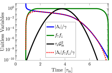
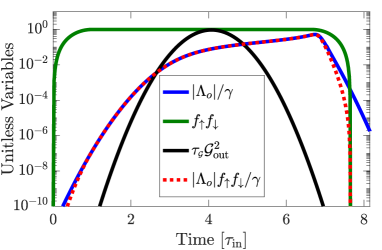
Figure 10: Illustration of the solutions for $|\Lambda_{i/o}|$ along with the smoothing functions in Eq. (173) that ensures well-behaved control fields. Parameters: (a) $\gamma\!=\!30\Omega_{\scriptscriptstyle\mathcal{G}}$, $\gamma_{L}\!=\!0$, $\tau_{\rm{e}}\!=\!\tau_{\!\scriptscriptstyle\mathcal{G}}$. (b) $\gamma_{L}\!=\!10^{-5}\Omega_{\scriptscriptstyle\mathcal{G}}$.

To avoid divergences and keep $|\Lambda_{i}|$ real, we multiply the solution in Eq. (142) by smoothing functions

$$f_{\uparrow}(t) =\frac{1\!+\!\sin\!\big{(}\frac{\pi t}{\tau_{\rm{e}}}\big{)}}{2}\Theta\Big{(}t\!+\!\frac{\tau_{\rm{e}}}{2}\Big{)}\Theta\Big{(}\frac{\tau_{\rm{e}}}{2}\!-\!t\Big{)}+\Theta\Big{(}t\!-\!\frac{\tau_{\rm{e}}}{2}\Big{)}$$ (173)

$$f_{\downarrow}(t) =\frac{1\!-\!\sin\!\big{(}\frac{\pi t}{\tau_{\rm{e}}}\big{)}}{2}\Theta\Big{(}t\!+\!\frac{\tau_{\rm{e}}}{2}\Big{)}\Theta\Big{(}\frac{\tau_{\rm{e}}}{2}\!-\!t\Big{)}+\Theta\Big{(}\!-\!\frac{\tau_{\rm{e}}}{2}\!-\!t\Big{)}$$ (174)

where $\Theta$ is a step function that equals 1 for positive arguments and 0 for negative arguments. The smoothing functions rise from 0 to 1 ($\uparrow$) or fall from 1 to 0 ($\downarrow$) in the interval $t\!\in\![-\tau_{\rm{e}}/2,~{}\tau_{\rm{e}}/2]$ as half a period of the sine function.

Appendix G Input Pump Fields for Absorption and Emission

The resonator modes that couple to the pump fields are identical and the Hamiltonian associated with those modes is

$$\hat{H}_{n}^{\rm{pump}}=i\hbar\sqrt{\frac{\gamma_{p}}{\Delta t}}\sum_{m=1}^{2}\!\Big{(}\hat{p}_{m}^{\dagger}\hat{W}_{n}-\hat{p}_{m}\hat{W}_{n}^{\dagger}\Big{)}+\hbar\hat{p}_{1}^{\dagger}\hat{p}_{1}\hat{p}_{2}^{\dagger}\hat{p}_{2}+\frac{1}{2}\hbar\!\sum_{m=1}^{2}\!\Big{(}\hat{p}_{m}^{\dagger}\hat{p}_{m}-1\Big{)}\hat{p}_{m}^{\dagger}\hat{p}_{m}.$$ (175)

The temporal shape of the input pump functions can be found by considering their equations of motion

$$\dot{\alpha}_{1} =\Big{(}-\frac{\Gamma_{p}}{2}-i\chi_{3}\big{(}|\alpha_{1}|^{2}+|\alpha_{2}|^{2}\big{)}\Big{)}\alpha_{1}+\sqrt{\gamma_{p}}\xi_{1}$$ (176a)

$$\dot{\alpha}_{2} =\Big{(}-\frac{\Gamma_{p}}{2}-i\chi_{3}\big{(}|\alpha_{1}|^{2}+|\alpha_{2}|^{2}\big{)}\Big{)}\alpha_{2}+\sqrt{\gamma_{p}}\xi_{2}.$$ (176b)

From Section III we have $\Lambda=\chi_{3}\alpha_{2}^{*}\alpha_{1}=|\Lambda|\exp(i\phi)\!=\!\chi_{3}r_{\!\alpha}^{2}\exp[i(\phi_{1}-\phi_{2})]$ and since we assumed $|\alpha_{1}|\!=\!|\alpha_{2}|$, we can express the complex amplitudes in polar form: $\alpha_{1}\!=\!r_{\!\alpha}\exp(i\phi_{1})$ and $\alpha_{2}\!=\!r_{\!\alpha}\exp(i\phi_{2})$, with $\phi\!=\!\phi_{1}-\phi_{2}$. The goal is to determine the complex-valued input fields, $\xi_{1}$ and $\xi_{2}$, such that Eq. (176) yields the correct intra-cavity control fields $\alpha_{1}$ and $\alpha_{2}$. Let us write the pump fields in polar form: $\xi_{n}\!=\!q_{n}\exp(i\psi_{n})$, and substitute into Eq. (176)

$$\dot{\alpha}_{n} =\big{(}\dot{r}_{\!\alpha}+i\dot{\phi}_{n}r_{\!\alpha}\big{)}e^{i\phi_{n}}=\big{(}-\frac{\Gamma_{p}}{2}-i2\chi_{3}r_{\!\alpha}^{2}\big{)}r_{\!\alpha}e^{i\phi_{n}}+\sqrt{\gamma_{p}}q_{n}e^{i\psi_{n}}.$$ (177)

Separating equations for the real and imaginary parts yields

$$\dot{r}_{\!\alpha} =-\frac{\Gamma_{p}}{2}r_{\!\alpha}+\sqrt{\gamma_{p}}q_{n}\cos(\psi_{n}-\phi_{n})$$ (178a)

$$\dot{\phi}_{n} =-2\chi_{3}r_{\!\alpha}^{2}+\sqrt{\gamma_{p}}\frac{q_{n}}{r_{\!\alpha}}\sin(\psi_{n}-\phi_{n}).$$ (178b)

Let us guess that $q_{1}\!=\!q_{2}\!=\!q$ and $\psi_{1}-\phi_{1}\!=\!-(\psi_{2}-\phi_{2})$. Since $\phi\!=\!\phi_{1}-\phi_{2}$, we have

$$\dot{\phi}=\dot{\phi}_{1}-\dot{\phi}_{2}=\sqrt{\gamma_{p}}\frac{q}{r_{\!\alpha}}\Big{[}\sin(\psi_{1}-\phi_{1})-\sin(\psi_{2}-\phi_{2})\Big{]}=2\sqrt{\gamma_{p}}\frac{q}{r_{\!\alpha}}\sin(\psi_{1}-\phi_{1})$$ (179)

Re-arranging Eqs. (178a) and (179), we have

$$\frac{1}{2}\frac{r_{\!\alpha}\dot{\phi}}{\big{(}\dot{r}_{\!\alpha}+\frac{\Gamma_{p}}{2}r_{\!\alpha}\big{)}}=\tan(\psi_{1}-\phi_{1}),~{}~{}\Rightarrow~{}~{}\psi_{1}-\phi_{1}=\arctan\!\Bigg{[}\frac{1}{2}\frac{r_{\!\alpha}\dot{\phi}}{\big{(}\dot{r}_{\!\alpha}+\frac{\Gamma_{p}}{2}r_{\!\alpha}\big{)}}\Bigg{]}.$$ (180)

Using the identity $\cos[\arctan(x)]\!=\!1/\sqrt{1+x^{2}}$, we find $q$ from Eq. (178a)

$$\dot{r}_{\!\alpha}+\frac{\Gamma_{p}}{2}r_{\!\alpha}=\sqrt{\gamma_{p}}q\frac{1}{\sqrt{1+\frac{1}{4}\Big{(}\frac{r_{\!\alpha}\dot{\phi}}{\dot{r}_{\!\alpha}+\frac{\Gamma_{p}}{2}r_{\!\alpha}}\Big{)}^{2}}},~{}~{}\Rightarrow~{}~{}q=\frac{1}{\sqrt{\gamma_{p}}}\sqrt{\Big{(}\dot{r}_{\!\alpha}+\frac{\Gamma_{p}}{2}r\Big{)}^{2}+\frac{\dot{\phi}^{2}r_{\!\alpha}^{2}}{4}}.$$ (181)

Using the identity $\sin[\arctan(x)]\!=\!x/\sqrt{1+x^{2}}$, we may insert Eq. (180) into Eq. (178b) to obtain

$$\dot{\phi}_{1} =-2\chi_{3}r_{\!\alpha}^{2}+\sqrt{\gamma_{p}}\frac{q}{r_{\!\alpha}}\Big{[}\frac{1}{2}\frac{r_{\!\alpha}\dot{\phi}}{\big{(}\dot{r}_{\!\alpha}+\frac{\Gamma_{p}}{2}r_{\!\alpha}\big{)}}\Big{]}\frac{1}{\sqrt{1+\frac{1}{4}\Big{(}\frac{r_{\!\alpha}\dot{\phi}}{\dot{r}_{\!\alpha}+\frac{\Gamma_{p}}{2}r_{\!\alpha}}\Big{)}^{2}}}=-2\chi_{3}r_{\!\alpha}^{2}+\frac{\dot{\phi}}{2}$$ (182a)

$$\dot{\phi}_{2} =-2\chi_{3}r_{\!\alpha}^{2}-\frac{\dot{\phi}}{2}.$$ (182b)

Integrating Eq. (182), and inserting into Eq. (180), we find

$$\psi_{1}(t) =-2\int_{0}^{t}\!|\Lambda(s)|ds+\frac{\phi(t)}{2}+\arctan\!\Bigg{[}\frac{1}{2}\frac{r_{\!\alpha}\dot{\phi}}{\big{(}\dot{r}_{\!\alpha}+\frac{\Gamma_{p}}{2}r_{\!\alpha}\big{)}}\Bigg{]}$$ (183a)

$$\psi_{2}(t) =-2\int_{0}^{t}\!|\Lambda(s)|ds-\frac{\phi(t)}{2}-\arctan\!\Bigg{[}\frac{1}{2}\frac{r_{\!\alpha}\dot{\phi}}{\big{(}\dot{r}_{\!\alpha}+\frac{\Gamma_{p}}{2}r_{\!\alpha}\big{)}}\Bigg{]}.$$ (183b)

References

- Kimble [2008] H. J. Kimble, The quantum internet., Nature 453, 1023 (2008).
- Hu and Weiss [2016] S. Huand S. M. Weiss, Design of Photonic Crystal Cavities for Extreme Light Concentration, ACS Photonics , acsphotonics.6b00219 (2016).
- Choi et al. [2017] H. Choi, M. Heuck, and D. Englund, Self-Similar Nanocavity Design with Ultrasmall Mode Volume for Single-Photon Nonlinearities, Physical Review Letters 118, 10.1103/PhysRevLett.118.223605 (2017).
- Hu et al. [2018] S. Hu, M. Khater, R. Salas-Montiel, E. Kratschmer, S. Engelmann, W. M. J. Green, and S. M. Weiss, Experimental Realization of Deep Subwavelength Confinement in Dielectric Optical Resonators, Science Advances 4 (2018), arXiv:1707.04672 .
- Zhang et al. [2019] M. Zhang, C. Wang, Y. Hu, A. Shams-Ansari, T. Ren, S. Fan, and M. Lončar, Electronically programmable photonic molecule, Nature Photonics 13, 36 (2019).
- Liang et al. [2017] H. Liang, R. Luo, Y. He, H. Jiang, and Q. Lin, High-quality lithium niobate photonic crystal nanocavities, Optica 4, 1251 (2017), arXiv:1706.08904 .
- Lenz et al. [2001] G. Lenz, B. J. Eggleton, C. K. Madsen, and R. E. Slusher, Optical delay lines based on optical filters, IEEE Journal of Quantum Electronics 37, 525 (2001).
- Tanaka et al. [2007] Y. Tanaka, J. Upham, T. Nagashima, T. Sugiya, T. Asano, and S. Noda, Dynamic control of the Q factor in a photonic crystal nanocavity, Nature materials 6, 862 (2007).
- Xu et al. [2007] Q. Xu, P. Dong, and M. Lipson, Breaking the delay-bandwidth limit in a photonic structure, Nature Physics 3, 406 (2007).
- McKinstrie et al. [2005] C. J. McKinstrie, J. D. Harvey, S. Radic, and M. G. Raymer, Translation of quantum states by four-wave mixing in fibers, Opt. Express 13, 9131 (2005).
- Li et al. [2016] Q. Li, M. Davanco, and K. Srinivasan, Efficient and low-noise single-photon-level frequency conversion interfaces using silicon nanophotonics, Nature Photonics 10, 406 (2016), arXiv:1510.02527 .
- Heuck et al. [2018] M. Heuck, J. G. Koefoed, J. B. Christensen, Y. Ding, L. H. Frandsen, K. Rottwitt, and L. K. Oxenlowe, Unidirectional frequency conversion in microring resonators for on-chip frequency-multiplexed single-photon sources, New Journal of Physics 21, 1 (2018), arXiv:1811.11741 .
- Guo et al. [2016] X. Guo, C.-L. Zou, H. Jung, and H. X. Tang, On-Chip Strong Coupling and Efficient Frequency Conversion between Telecom and Visible Optical Modes, Physical Review Letters 117, 123902 (2016).
- Madsen et al. [1999] C. K. Madsen, G. Lenz, A. J. Bruce, M. A. Cappuzzo, L. T. Gomez, and R. E. Scotti, Integrated all-pass filters for tunable dispersion and dispersion slope compensation, IEEE Photonics Technology Letters 11, 1623 (1999).
- Scarani et al. [2002] V. Scarani, M. Ziman, P. Štelmachovič, N. Gisin, and V. Bužek, Thermalizing quantum machines: Dissipation and entanglement, Physical Review Letters 88, 097905 (2002).
- Ciccarello [2017] F. Ciccarello, Collision models in quantum optics, Quantum Measurements and Quantum Metrology 4, 53 (2017).
- Gross et al. [2018] J. A. Gross, C. M. Caves, G. J. Milburn, and J. Combes, Qubit models of weak continuous measurements: markovian conditional and open-system dynamics, Quantum Science and Technology 3, 024005 (2018).
- Vernon et al. [2016] Z. Vernon, M. Liscidini, and J. E. Sipe, Quantum frequency conversion and strong coupling of photonic modes using four-wave mixing in integrated microresonators, Physical Review A 94, 1 (2016), arXiv:1606.01582 .
- Haus [1984] H. A. Haus, Waves and Fields in Optoelectronics, 1st ed. (Prentice-Hall, 1984).
- Jacobs [2014] K. Jacobs, Quantum measurement theory and its applications (Cambridge University Press, Cambridge, 2014).
- Knill et al. [2001] E. Knill, G. Milburn, and R. Laflamme, A scheme for efficient quantum computation with linear optics, Nature 409, 46 (2001), arXiv:arXiv:1208.4575v2 .
- Nysteen et al. [2017] A. Nysteen, D. P. S. McCutcheon, M. Heuck, J. Mørk, and D. R. Englund, Limitations of two-level emitters as nonlinearities in two-photon controlled-PHASE gates, Physical Review A 95, 1 (2017), arXiv:1612.04803 .
- Cirac et al. [1996] J. I. Cirac, P. Zoller, H. J. Kimble, and H. Mabuchi, Quantum state transfer and entanglement distribution among distant nodes in a quantum network, Physical Review Letters , 3221 (1996), arXiv:9611017 [quant-ph] .
- Gronwall [1919] T. H. Gronwall, Note on the derivatives with respect to a parameter of the solutions of a system of differential equations, Annals of Mathematics 20, 292 (1919).