Fundamental bounds on rotational state change
in sympathetic cooling of molecular ions

Abstract

Sympathetic cooling of molecular ions through the Coulomb interaction with laser-cooled atomic ions is an efficient tool to prepare translationally cold molecules. Even at relatively high collisional energies of about 1 eV ($T\sim 10000\,$K), the nearest approach in the ion-ion collisions never gets closer than $\sim$$1\,$nm such that naively perturbations of the internal molecular state are not expected. The Coulomb field may, however, induce rotational transitions changing the purity of initially quantum state prepared molecules. Here, we investigate such rotational state changing collisions for both polar and apolar diatomic molecular ions and derive closed-form estimates for rotational excitation based on the initial scattering energy and the molecular parameters.

Cold molecule science is a growing field of research with perspectives ranging from the test of fundamental physics or chemistry in the ultra-cold regime all the way to quantum information processing Bohn et al. (2017); Dulieu and Osterwalder (2018); Krems (2018). One interesting avenue to realize such goals is to experiment with cold molecular ions, since essentially any molecular ion with initial kinetic energy of $10\,$eV or lower can be trapped and sympathetically cooled through the Coulomb interaction with laser-cooled atomic ions Mølhave and Drewsen (2000). A variety of diatomic polar Mølhave and Drewsen (2000); Koelemeij et al. (2007); Staanum et al. (2008); Willitsch et al. (2008); Hansen et al. (2012) and apolar Blythe et al. (2005); Tong et al. (2010) as well as larger molecular ions Ostendorf et al. (2006); Højbjerre et al. (2008) have been cooled this way to a few tens of millikelvin. Single molecular ions have been cooled to the ground state of their collective motion with a single co-trapped and laser-cooled atomic ion Wan et al. (2015); Rugango et al. (2015); Wolf et al. (2016); wen Chou et al. (2017). Simultaneously, optical pumping Vogelius et al. (2002); Staanum et al. (2010); Schneider et al. (2010); Deb et al. (2013), helium buffer gas cooling Hansen et al. (2014), probabilistic state preparation Wolf et al. (2016); wen Chou et al. (2017) and resonance enhanced multi-photon ionization (REMPI) Tong et al. (2010); Gardner et al. (2019) have been applied to produce molecular ions in specific internal states with high probability. The latter method differs from the others in that the internal quantum state is prepared prior to sympathetic translational cooling and may thus be prone to state changes during cooling. So far, it has only been applied to form state-selected N${}_{2}^{+}$ molecules in the vicinity of the trap potential minimum Tong et al. (2010). This is, however, not possible in general, for example in cases where the neutral precursor molecule (such as H₂ or HD) reacts efficiently with the laser-cooled atomic ions. It is then necessary to first produce the state-selected molecular ions in one trap and transfer them into another trap more suitable for translational sympathetic cooling. A similar situation is encountered for molecular ions that have to be produced by an external source, such as an electrospray ion source combined with an internal state pre-cooling trap Stockett et al. (2016). In these cases, the initial kinetic energy of the captured molecular ions can be as high as the effective trap potential, typically in the $1-10\,$eV range. Even though close encounter collisions, where the distance between the collision partners becomes comparable to or smaller than the size of the particles’ wavefunctions, are energetically suppressed by the ion-ion repulsion, internal state change may be induced by the Coulomb field of the atomic ions at the position of the molecular ion.

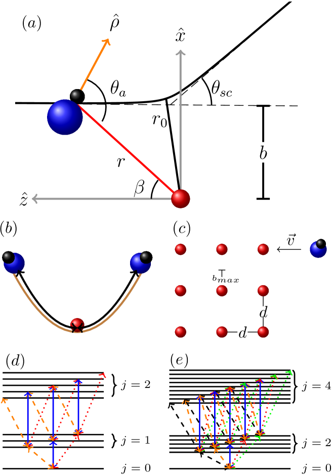
Figure 1: Sympathetic cooling of a molecular ion via collisions with laser-cooled atomic ions: Scattering geometry (a) and the considered cooling scenarios with either a single trapped atom (b) or many atomic ions forming a Coulomb crystal (c). Rotational excitations are due to the Coulomb interaction, with the selection rules for polar and apolar molecules shown in (d), respectively (e). For head-on collisions only $\Delta m=0$ (blue arrows) are allowed.

Here, we estimate the probability of rotational state change as a function of the collisional energy for collisions between atomic ions and polar/apolar diatomic molecules initially prepared in their rovibrational ground state . We also estimate the number of collisions required to reach a certain final translational energy. By combining these results, we are able to estimate the probability of rotational excitation during sympathetic cooling. Our model is built on a separation of energy scales for relative and internal molecular motion: While initial scattering energies range from $0.1\,$eV to 10 eV, the rotational energy scale is only of the order of $10^{-4}\,$eV. Hence, we treat the relative motion classically Hashemloo and Dion (2015); Hashemloo et al. (2016), as depicted in Fig. 1(a). In contrast, the rotational excitations are described fully quantum mechanically, with possible transitions indicated in Fig. 1(d) and (e). Vibrations of the molecule do not play any role. We inspect two cooling regimes, illustrated in Fig. 1(b) and (c): The trap, assumed to be harmonic and isotropic, can either contain a single atomic ion Staanum et al. (2008); Hansen et al. (2012); Tong et al. (2010) or many atomic ions that form a Coulomb crystal Staanum et al. (2010); Heazlewood and Softley (2015). This will be important for the time required to reach the final energy.

Treating the molecule as a point particle, the relative motion reduces to the textbook problem of classical scattering in a $1/r$-potential Goldstein (1980). This neglects the trap potential which is reasonable at the relevant short distances. Classical scattering is characterized by the impact parameter $b$ which is not fixed in a sympathetic cooling experiment. We thus need to average over all possible values of $b$. In the case of cooling by a single atom (SA), cf. Fig. 1(b), we assume the atom to be in the trap ground state. The distribution of impact parameters is then given by

$$f_{SA}(b)=\frac{b}{\sigma^{2}}e^{-\frac{b^{2}}{2\sigma^{2}}}\,,$$ (1)

where $\sigma=\sqrt{E/\left(\mu\omega^{2}\right)}$ is the effective length of the trap at a given energy, $\omega$ the trap frequency and $\mu=\frac{m_{mol}M_{atom}}{M+{mol}+M_{atom}}$ the reduced mass with $M_{mol}$ and $M_{atom}$ the molecular and atomic masses. In the second scenario, that of a large Coulomb crystal (CC), the lattice spacing $d$ determines the maximum impact parameter in a scattering event, $b_{max}=d/2$. Assuming a regular lattice, cf. Fig. 1(c), we can approximate the distribution by

$$f_{CC}(b)=\frac{2b}{b^{2}_{max}},\quad b\in[0,b_{max}]\,,$$ (2)

Using Eqs. (1) and (2), we determine, in the supplemental material (SM) SM , the total time required to lower the molecule’s energy from $E_{lab,1}$ to $E_{lab,N}$,

$$T = \sum_{i=1}^{N}n(E_{lab,i})\tau\,,$$ (3)

where $n(E_{lab,i})$ is the number of scattering events to change the energy from $E_{lab,i}$ to $E_{lab,i+1}$ and $\tau$ the time between collisions. We can thus establish, from Eqs. (6) and (9) in SM , a simple relation between the cooling times in the two regimes, namely

$$\frac{T_{SA}}{T_{CC}}\sim\left(\frac{\sigma_{1}}{d}\right)^{3}\,.$$ (4)

For standard Coulomb crystals, $d\approx 10\,\mu$m, whereas $\sigma=635\,\mu$m for $E_{lab}=2\,$eV. With $\omega=2\pi\times 1\,$MHz, $T_{SA}$ is more than $10^{6}$ times larger than $T_{CC}$. As an example, cooling ²⁴MgH⁺ from $2\,$eV to $0.01\,$eV in a crystal of ²⁴Mg⁺ with $d=5.29\,\mu$m takes approximately $2\,$ms in agreement with an earlier estimate Bussmann et al. (2006), compared to $\sim$$1\,$hour when cooling with a single atomic ion. Sympathetic translational cooling is thus much more advantageous in a Coulomb crystal, and we solely focus on this scenario now.

In order to estimate the rotational excitation over a complete cooling cycle with repeated collisions, we discretize the range from the initial to the final scattering energy, analogously to Eq. (3). The population excitation in a single collision with energy $E$ and impact parameter $b$ is $\epsilon(E,b)=1-P_{0}(E,b)$, where $P_{0}(E,b)$ is the remaining ground state population after the collision. Averaging over all impact parameters, $\tilde{\epsilon}(E)=\Braket{\epsilon(E,b)}$, the remaining ground state population in energy subinterval $i$ is approximately given by

$$P_{i} = (1-\tilde{\epsilon}(E_{i}))^{n(E_{i})}=\sum_{k=0}^{n(E_{i})}\frac{n(E_{i})!}{k!(n(E_{i})-k)!}\tilde{\epsilon}(E_{i})^{k}$$ (5)

$$= 1-n(E_{i})\tilde{\epsilon}(E_{i})+\frac{n(E_{i})(n(E_{i})-1)}{2}\tilde{\epsilon}(E_{i})^{2}\mp...$$

$$\approx 1-n(E_{i})\tilde{\epsilon}(E_{i})\,.$$

The population remaining in the ground state after the full cycle is obtained as $P=\Pi_{i=1}^{N}P_{i}$. Thus the population excited out of the ground state during the full cycle, $\Sigma=1-P$, can be estimated to first order in $n(E_{i})\tilde{\epsilon}(E_{i})$,

$$\Sigma\approx\sum_{i=1}^{N}n(E_{i})\tilde{\epsilon}(E_{i})\,.$$ (6)

Population excitation in a single collision may be caused by the atomic ion generating an electric field that affects the rotational dynamics of the molecular ion. The relative motion results in an effectively time-dependent field, the profile of which can very well be approximated by a Lorentzian, $\varepsilon(t)=\frac{E^{2}\left(\tau/2\right)^{2}}{t^{2}+\left(\tau/2\right)^{2}}$ with full width at half maximum $\tau=1.86\sqrt{\mu/E^{3}}$. To leading order, the molecule couples to the field via its dipole moment in the case of polar molecules, or, for apolar molecules, via its polarizability anisotropy or quadrupole moment. For polar molecules, when disregarding the quadrupole interaction, the Hamiltonian governing the rotational dynamics is given by

$$\boldsymbol{\mathbf{\hat{H}}}_{p} = B\boldsymbol{\mathbf{\hat{J}}}^{2}-D\varepsilon(t)\cos{\boldsymbol{\mathbf{\hat{\theta}}}_{a}}$$

$$= B\boldsymbol{\mathbf{\hat{J}}}^{2}-D\varepsilon(t)\left(\cos{\beta}\cos{\boldsymbol{\mathbf{\hat{\theta}}}}+\sin{\beta}\sin{\boldsymbol{\mathbf{\hat{\theta}}}}\cos{\boldsymbol{\mathbf{\hat{\phi}}}}\right),$$

where $B$ is the rotational constant, $D$ the dipole moment, $\phi$ the azimutal angle around the molecular axis, $\theta_{a}$ the angle between molecular axis and electric field vector, and $\beta$ the angle between molecule and fixed scattering center in the CM frame, cf. Fig. 1(a). The Hamiltonian for apolar molecules reads

$$\boldsymbol{\mathbf{\hat{H}}}_{ap} = B\boldsymbol{\mathbf{\hat{J}}}^{2}-\frac{\varepsilon^{2}(t)}{4}\left(\Delta\alpha\cos^{2}{\boldsymbol{\mathbf{\hat{\theta}}}_{a}}+\alpha_{\perp}\right)$$ (8)

$$+\frac{Q_{Z}\varepsilon^{3/2}(t)}{4}\left(3\cos^{2}{\boldsymbol{\mathbf{\hat{\theta}}}_{a}}+1\right)\,,$$

where $\boldsymbol{\mathbf{\hat{\theta}}}_{a}$ can be substituted in terms of $\beta$, $\boldsymbol{\mathbf{\hat{\theta}}}$ and $\boldsymbol{\mathbf{\hat{\phi}}}$, similar to Eq. (Fundamental bounds on rotational state change in sympathetic cooling of molecular ions), $\Delta\alpha$ is the polarizability anisotropy, $\alpha_{\perp}$ the polarizability perpendicular to the molecular axis, and $Q_{Z}$ the quadrupole moment along the axis. In both cases, the angle $\beta$ is given by the classical trajectory,

$$\beta = \int_{r}^{\infty}\frac{b\,ds}{s^{2}\sqrt{\left(1-\frac{V(s)}{E}\right)-\frac{b^{2}}{s^{2}}}}\;\;\mathrm{for}\;t<0,$$

$$\beta = \int_{r_{0}}^{\infty}\frac{b\,ds}{s^{2}\sqrt{\left(1-\frac{V(s)}{E}\right)-\frac{b^{2}}{s^{2}}}}+\int_{r_{0}}^{r}\frac{b\,ds}{s^{2}\sqrt{\left(1-\frac{V(s)}{E}\right)-\frac{b^{2}}{s^{2}}}}$$

$$\quad\quad\quad\quad\quad\quad\quad\quad\quad\quad\quad\quad\mathrm{for}\;t>0.$$

with $r\in[r_{0},\infty]$ and $r_{0}$ the minimal distance the collisions partners can reach, cf. Fig. 1(a). The dynamics can be characterized in terms of the ratio of maximum interaction strength to rotational kinetic energy for the three types of coupling,

$$\chi_{D}=\frac{D\varepsilon_{0}}{B}\,,\quad\chi_{\alpha}=\frac{\Delta\alpha\varepsilon_{0}^{2}}{4B},\quad\chi_{Q}=\frac{3Q_{Z}\varepsilon_{0}^{3/2}}{4B}\,.$$ (9)

This explains why we have omitted the quadrupole interaction in Eq. (Fundamental bounds on rotational state change in sympathetic cooling of molecular ions): For head-on collisions, when the interaction is strongest, $\frac{\chi_{Q}}{\chi_{D}}=\frac{3Q_{Z}}{4D}E$ is equal to $0.013E$ (in eV) for MgH⁺ and $0.11E$ for HD⁺. In contrast, for apolar molecules and head-on collisions the quadrupole interaction dominates, for example, for N${}_{2}^{+}$ at 2 eV $\frac{\chi_{Q}}{\chi_{\alpha}}\approx 8$. The long-range behavior also favors the quadrupole interaction but for completeness we account for both types of interaction in Eq. (8).

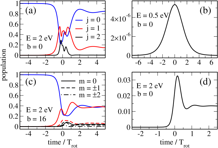
Figure 2: Rotational dynamics during one scattering event with energy $E$ and impact parameter $b$ for HD⁺/Be⁺ (a,c) and H${}_{2}^{+}$/Be⁺ (b,d). The impact parameter in (c) is the one resulting in most excitation, whereas for apolar molecules maximum excitation always occurs for $b=0$. The collision involves adiabatic dynamics in panels (a), (b) and non-adiabatic dynamics in (c), (d). The dynamics is qualitatively the same for other polar and apolar molecular species.

Figure 2 illustrates the rotational dynamics during one scattering event. For polar molecules and head-on collisions, cf. Fig. 2(a), the population excitation at intermediate times becomes rather large, but most population returns to the ground state after the collision. This dynamics can be visualized in terms of the molecule aligning itself almost adiabatically with the electric field. Due to the more complex interaction for non-zero $b$, the excited state population does not return as easily to the ground state, cf. Fig. 2(c). In contrast, for apolar molecules, the largest final excitation is found for head-on collisions, but overall the excitation is much smaller than for polar molecules. These observations suggest to analyze the rotational dynamics in terms of non-adiabaticity for polar molecules and perturbation theory for apolar ones.

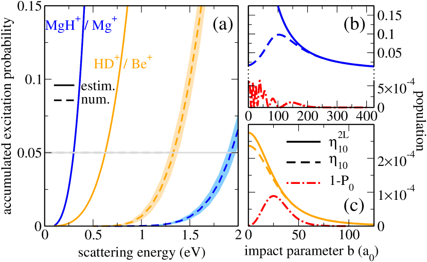
Figure 3: (a) Accumulated excitation probability, Eq. (6), for polar molecules after a full cooling cycle, as a function of the initial scattering energy with $E_{final}=0.1\,$eV, comparing the estimate (solid lines) based on approximation (11) (with $dE=0.05\,$eV) to full numerical simulations (dashed lines, $dE=0.1$ eV). Within each interval $dE$, the excitation occuring in a single collision, $\tilde{\epsilon}$, can be evaluated at the highest and lowest energy, $E_{i}$ and $E_{i}-dE$, defining the shaded region, or taken to be the arithmetic mean, indicated by the dashed lines. The horizontal gray line marks an excitation level of 5%. (b), (c) Population excited in a single collision (red dot-dashed line) together with the exact (dashed lines) and approximated (solid lines) non-adiabaticity measures, cf. Eqs. (10) and (11), as a function of the impact parameter at a scattering energy of $1\,$eV ($d=1\times 10^{5}\,$Bohr) for MgH⁺ (b) and HD⁺ (c).

Non-adiabaticity of the dynamics can be measured by

$$\eta_{\iota^{\prime}\iota}=\frac{\Braket{\iota^{\prime}(t)}{\frac{\partial\boldsymbol{\mathbf{\hat{H}}}_{p}}{\partial t}}{\iota(t)}}{\left(E_{\iota^{\prime}}(t)-E_{\iota}(t)\right)^{2}}\,,$$ (10)

where $\eta_{\iota^{\prime}\iota}=0$ corresponds to fully adiabatic dynamics, $E_{\iota}(t)$ are the instantaneous eigenvalues and $\{\Ket{\iota(t)}\}$ the instantaneous eigenstates of $\boldsymbol{\mathbf{\hat{H}}}_{p}(t)$. Considering the lowest two instantaneous eigenstates only and evaluating the field at $t=\frac{\tau}{2}$ results in an estimate of $\eta_{\iota^{\prime}\iota}$ that depends solely on the molecular parameters,

$$\eta^{2L}_{10}=\frac{\chi_{D}(b,E)}{4\cdot 1.86\sqrt{\frac{\mu}{E^{3}}}B\left(1+\left(\frac{\chi_{D}(b,E)}{2\sqrt{3}}\right)^{2}\right)}\frac{1}{\sqrt{3}}\,.$$ (11)

$\eta^{2L}_{10}$ can be directly related to the amplitude of the first excited instantaneous eigenstate, i.e., to the population excited in a single collision Ballentine (1998), see also the SM SM . Averaging $\eta^{2L}_{10}$ over the impact parameter and inserting the result into Eq. (6) thus yields an upper bound of the excited population at the end of the cooling process. This is shown in Fig. 3(a). Comparison with numerical simulations show that the bound is tighter for HD⁺/Be⁺ than for MgH⁺/Mg⁺. This is in agreement with the two-level approximation being fairly faithful for HD⁺/Be⁺, cf. Fig. 3(c), in contrast to MgH⁺/Mg⁺, cf. Fig. 3(b), where the bound clearly overestimates the excitation probability. Our simulations indicate that significant population excitation (of a few percent or more) begins to occur at initial scattering energies of $1.75\,$eV for MgH⁺/Mg⁺ and $1\,$eV for HD⁺/Be⁺, in contrast to about $0.25\,$eV, resp. $0.5\,$eV, predicted by the estimate (11) using only the molecular parameters. We therefore conclude that the non-adiabaticity parameter gives a very conservative estimate, in particular for molecular ions with a large value of $\chi_{D}$.

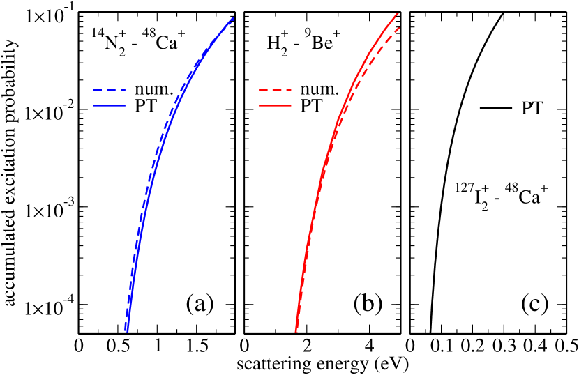
Figure 4: Accumulated excitation for apolar molecular ions after a full cooling cycle as function of the initial scattering energy, comparing full numerical calculations (dashed lines) to PT (solid lines, $d=1\times 10^{5}$ Bohr).

For apolar molecules, an estimate for the rotational excitation after one collision can be obtained using first-order time-dependent perturbation theory (PT). The corresponding integrals over time can be evaluated numerically or approximated by an analytical fit SM . Averaging over the impact parameter for each collision and accumulating over all collisions according to Eq. (6) results in an estimate for the population that is excited at the end of the cooling process solely in terms of the molecular parameters,

$$\Sigma \approx 1.86^{2}\frac{3(1+\xi)^{2}\mu Q_{Z}^{2}}{200\xi}\times$$

$$\int_{E_{i}}^{E_{f}}\frac{E^{2}\left(1+1.86a_{1}\sqrt{\frac{\mu}{E^{3}}}B\right)^{2a_{2}}e^{-2a_{3}1.86\sqrt{\frac{\mu}{E^{3}}}B}}{\log{\left(\left(d\cdot E\right)^{2}+1\right)}}dE\,,$$

where $\xi$ is the ratio of the molecular to the atomic mass and $a_{i}$ are the fit parameters SM . For simplicity, we have only accounted for the dominant quadrupole interaction in the PT. Figure 4(a) and (b) compares the results obtained with PT and the full dynamics using Eq. (8), confirming both validity of PT and insignificance of the polarizability interaction for N${}_{2}^{+}$/Ca⁺ and H${}_{2}^{+}$/Be⁺. This suggests to use Eq. (Fundamental bounds on rotational state change in sympathetic cooling of molecular ions) to make predictions for other molecular species, such as iodine, shown in Fig. 4(c). For the popular example of N${}_{2}^{+}$ Tong et al. (2010); Germann et al. (2014); Germann and Willitsch (2016a, b), we expect excitation of more than a few percent only for initial scattering energies well above 1.5 eV. However, for very heavy molecules with small rotational constants, such as I${}_{2}^{+}$, significant rotational excitation is expected already for initial energies of a few hundred meV. In Fig. 4 we have assumed $d=1\times 10^{5}$ Bohr but numerical simulations suggest the final excitation probability to only very weakly depend on the value of $d$ or even on the cooling scenario. The total cooling time, however, strongly depends on the particular scenario and values of $d$ as explained above.

In conclusion, predicting the rotational excitation of diatomic molecular ions during sympathetic cooling by laser-cooled atomic ions requires a full quantum-dynamical treatment for polar molecules, whereas validity of PT for apolar molecules has allowed us to derive a closed-form estimate of the accumulated population excitation which solely depends on the molecular parameters and initial scattering energy. The scenarios of using a Coulomb crystal of atomic ions or just a single atomic ion do not significantly change the final degree of collision-induced rotational excitation. However, translational cooling with a single atomic ion is dramatically slower and will generally be impractical. For a wide range of apolar molecules, we find the internal state to be preserved for initial energies of 1 eV and above, eventually limited by close-encounter interactions disregarded in the present treatment. When extending sympathetic cooling to polyatomics, we expect rotational excitation to be more critical, both because of more degrees of freedom with low-energy spacings and the physical size of the molecules making close-encounter interactions more likely. The latter deserve a more thorough investigation in future work as they might provide a new avenue for controlling collisions due to the extremely large fields present in a close encounter. The control knob would be the initial collision energy which can be varied via the choice of the molecule’s position in the trap during photo-ionization, or by injecting low-energetic molecular ions from an external source into the trap. The same techniques could also be used to experimentally test our present predictions for diatomics.

Supplementary material
Fundamental bounds on rotational state change
in sympathetic cooling of molecular ions

J. Martin Berglund, Michael Drewsen, Christiane P. Koch

.1 Classical description of the translational motion

The energy transferred from the molecule to the atom (in the laboratory frame) in a single scattering event, $dE_{lab}$, is determined by the initial energy, $E_{lab}$, the mass ratio $\xi=M_{mol}/M_{at}$ and the scattering angle $\theta_{sc}$,

$$dE_{lab}=\frac{2\xi(1-\cos{\theta_{sc}})}{(1+\xi)^{2}}E_{lab}\,.$$ (1)

The latter depends on the scattering energy $E$ (in the center-of-mass (CM) frame) $E$ and the impact parameter $b$, cf. Fig. 1 in the main text, $\theta_{sc}(E,b)=2\sin^{-1}{\left(1/\sqrt{1+\left(2Eb\right)^{2}}\right)}$. The CM and lab frame energies are related by $E_{lab}=EM_{mol}/\mu$ for elastic collisions, with reduced mass $\mu=\frac{M_{mol}M_{at}}{M_{mol}+M_{at}}$. The mean energy loss of the molecular ion in one scattering event is obtained by averaging over $b$,

$$\Braket{dE_{lab}(E_{lab})}=\int_{0}^{\infty}dE_{lab}(E_{lab},b)\,f(b)\,b\,db\,,$$ (2)

where the probability distribution $f(b)$ depends on the specific cooling scenario. In the single atom cooling case with $\sigma$, cf. Eq. (1) in the main text, large compared to $b$, which is true for the relevant impact parameters, we find

$$\Braket{dE_{lab}(E_{lab})}_{SA} = \frac{1}{\sigma^{2}}\int_{0}^{\infty}dE_{lab}(E_{lab},b)e^{-\frac{b^{2}}{2\sigma^{2}}}bdb,$$ (3)

$$\approx \frac{\xi\log{((2\sigma E_{lab})^{2}+1)}}{(1+\xi)^{2}\sigma^{2}E_{lab}}.$$

Using Eq. (3), the number of scattering events required to change the translational energy of the molecule by $\Delta E_{lab}$ is given by

$$n_{SA}(E_{lab}) = \frac{\Delta E_{lab}}{\Braket{dE_{lab}(E_{lab})}}_{SA}$$ (4)

$$\approx \frac{(1+\xi)^{2}\sigma^{2}E_{lab}}{\xi\log{((2\sigma E_{lab})^{2}+1)}}\Delta E_{lab}.$$

Since the molecular ion oscillates in the trap, the time between two scattering events amounts to $\tau_{SA}=\frac{\pi}{\omega}$, independent of $E_{lab}$. Discretizing the energy range, the total time needed to lower the molecule’s energy by $\Delta E_{lab}$ can be approximated by

$$T_{SA} = \sum_{i=1}^{N}n_{SA}(E_{lab,i})\tau_{SA}=\frac{\pi}{\omega}\sum_{i=1}^{N}n_{SA}(E_{lab,i})$$ (5)

$$= \pi\sqrt{\mu}\sum_{i=1}^{N}\frac{(1+\xi)^{2}\sigma_{i}^{3}\sqrt{E_{lab,i}}}{\xi\log{((2\sigma_{i}E_{lab,i})^{2}+1)}}\Delta E_{i}$$

with $\sigma_{i}=\sqrt{\frac{E_{lab,i}}{\mu\omega^{2}}}$. From Eq. (5), it is clear that cooling at the highest energies is much slower than at low energies. We may thus approximate the total cooling time,

$$T_{SA}\leq\pi\sqrt{\mu}\sigma_{1}^{3}\sum_{i=1}^{N}\frac{(1+\xi)^{2}\sqrt{E_{lab,i}}}{\xi\log{((2\sigma_{1}E_{lab,i})^{2}+1)}}\Delta E_{i}.$$ (6)

In the second scenario, cooling in a Coulomb crystal, the mean energy loss becomes

$$\Braket{dE_{lab}(E_{lab})}_{CC}=\frac{4\xi\log{((d\cdot E_{lab})^{2}+1)}}{(1+\xi)^{2}d^{2}E_{lab}}\,.$$ (7)

With the time between collisions now given by

$$\tau_{CC}=\frac{d}{v_{lab}}=d\sqrt{\frac{\mu}{2E_{lab}}},$$ (8)

the total cooling time becomes

$$T_{CC}=d^{3}\sqrt{\frac{\mu}{2}}\sum_{i=1}^{N}\frac{(1+\xi)^{2}\sqrt{E_{lab,i}}}{4\xi\log{((d\cdot E_{lab,i})^{2}+1)}}\Delta E_{i}.$$ (9)

Equations (6) and (9) yield Eq. (4) in the main text.

.2 Molecular model

For completeness, we present the Hamiltonian for apolar molecules, Eq. (8) in the main text, with $\boldsymbol{\mathbf{\hat{\theta}}}_{a}$ substituted by $\beta$, $\boldsymbol{\mathbf{\hat{\theta}}}$ and $\boldsymbol{\mathbf{\hat{\phi}}}$. It reads

$$\boldsymbol{\mathbf{\hat{H}}}_{ap} = B\boldsymbol{\mathbf{\hat{J}}}^{2}-\frac{\varepsilon^{2}(t)}{4}\Big{[}\Delta\alpha\Big{(}\cos^{2}{\beta}\cos^{2}{\boldsymbol{\mathbf{\hat{\theta}}}}+2\cos{\beta}\sin{\beta}\cos{\boldsymbol{\mathbf{\hat{\theta}}}}\sin{\boldsymbol{\mathbf{\hat{\theta}}}}\cos{\boldsymbol{\mathbf{\hat{\phi}}}}+\sin^{2}{\beta}\sin^{2}{\boldsymbol{\mathbf{\hat{\theta}}}}\cos^{2}{\boldsymbol{\mathbf{\hat{\phi}}}}\Big{)}+\alpha_{\perp}\Big{]}$$ (10)

$$+\frac{Q_{Z}\varepsilon^{3/2}(t)}{4}\left[3\left(\cos^{2}{\beta}\cos^{2}{\boldsymbol{\mathbf{\hat{\theta}}}}+2\cos{\beta}\sin{\beta}\cos{\boldsymbol{\mathbf{\hat{\theta}}}}\sin{\boldsymbol{\mathbf{\hat{\theta}}}}\cos{\boldsymbol{\mathbf{\hat{\phi}}}}+\sin^{2}{\beta}\sin^{2}{\boldsymbol{\mathbf{\hat{\theta}}}}\cos^{2}{\boldsymbol{\mathbf{\hat{\phi}}}}\right)+1\right].$$

	$10^{-5}$B	D	$\Delta\alpha$	$\alpha_{\perp}$	$Q_{Z}$	$\mu$
24MgH+	2.88	1.18	-	-	0.562 (∗)	22473.21
HD+	9.96	0.34	-	-	$\approx 1.39$ (∗∗)	4155.36
14N${}_{2}^{+}$	0.90	-	9.12	9.62	1.741	32463.57
H${}_{2}^{+}$	12.69	-	3.72	1.71	1.39	3024.57
127I${}_{2}^{+}$	0.015	-	55.64	XX	11.211	74056.55

Table 1: Rotational constant $B$, dipole moment $D$, polarizability anisotropy $\Delta\alpha$, and quadrupole moment $Q_{Z}$ of a few molecular ions as well as reduced mass $\mu$ of molecular ion and coolant (²⁴MgH⁺ for MgH⁺, ⁹Be⁺ for HD⁺, H${}_{2}^{+}$, ⁴⁸Ca⁺ for N${}_{2}^{+}$ and I${}_{2}^{+}$), all in atomic units. ^∗ very varying values between methods at NIST. ^∗∗ No values cited at NIST, we use the value given for H${}_{2}^{+}$ NIST (2018).

In our calculations, we have employed the molecular parameters as listed in Table 1.

.3 Adiabatic theory for polar molecules

Consider the instantaneous eigenstates $\Ket{\psi_{n}(t)}$ of a time-dependent Hamiltonian $\boldsymbol{\mathbf{\hat{H}}}(t)$,

$$\boldsymbol{\mathbf{\hat{H}}}(t)\Ket{\psi_{n}(t)}=E_{n}(t)\Ket{\psi_{n}(t)},$$ (11)

with eigenenergies $E_{n}(t)$. Any state $\Ket{\Psi(t)}$ can be expanded into the time-dependent eigenstates, $\Ket{\Psi(t)}=\sum_{n}c_{n}e^{i\Theta_{n}(t)}\Ket{\psi_{n}(t)}$, where $\Theta_{n}=-\int^{t}E_{n}(t^{\prime})dt^{\prime}$. Inserting the expansion of $\Ket{\Psi(t)}$ into the time-dependent Schrödinger equation,

$$i\partial_{t}\Ket{\psi(t)}=\boldsymbol{\mathbf{\hat{H}}}\Ket{\psi(t)}\,,$$ (12)

and multiplying both sides by $\Bra{\psi_{m}(t)}$, we obtain

$$\dot{c}_{m}(t)=-\sum_{n}c_{n}(t)e^{i\Delta\Theta_{nm}(t)}\Braket{\psi_{m}(t)}{\dot{\psi}_{n}(t)}.$$ (13)

Differentiating Eq. (11) w.r.t. time, we find

$$\Braket{\psi_{m}(t)}{\dot{\psi}_{n}(t)}=\frac{\Braket{\psi_{m}(t)}{\partial_{t}\boldsymbol{\mathbf{\hat{H}}}(t)}{\psi_{n}(t)}}{E_{n}(t)-E_{m}(t)},\qquad n\neq m,$$ (14)

where we have used $\Braket{\psi_{m}(t)}{\psi_{n}(t)}=\delta_{mn}$. If, at any given collision, the actual excitation is small, it is sufficient to consider only the two lowest levels. Assuming almost adiabatic dynamics, $c_{0}(t)\sim 1$ and $c_{1}(t)\sim 0$, we can integrate Eq. (13),

$$c_{1}(t)\approx\int_{-\infty}^{t}e^{i\Delta\Theta_{01}(t^{\prime})}\frac{\Braket{\psi_{1}(t^{\prime})}{\partial_{t}\boldsymbol{\mathbf{\hat{H}}}(t^{\prime})}{\psi_{0}(t^{\prime})}}{E_{1}(t^{\prime})-E_{0}(t^{\prime})}dt^{\prime}.$$ (15)

Simulations suggest that the main population transfer occurs at times $t\sim\pm\frac{\tau}{2}$. We then make the approximation that $\Braket{\psi_{1}(t)}{\partial_{t}\boldsymbol{\mathbf{\hat{H}}}}{\psi_{0}(t)}$ and $E_{1}-E_{0}=$ const. and evaluate the constant at $t=\frac{\tau}{2}$. In addition, we approximate $\Delta\Theta_{01}(t)$ by the time-independent eigenenergies, $(E_{1}-E_{0})t$. Since the population excitation is negligible for $|t|>\frac{\tau}{2}$ we can take the limits of integration to be between $\pm\frac{\tau}{2}$ and obtain

$$c_{1}\approx\frac{\Braket{\psi_{1}(t)}{\partial_{t}\boldsymbol{\mathbf{\hat{H}}}(t)}{\psi_{0}(t)}}{(E_{1}(t)-E_{0}(t))^{2}}2\cos{\frac{\tau}{2}\Delta E_{10}}\,.$$ (16)

We have thus found a relation between the population excitation in a single collision and the non-adiabaticity parameter,

$$|c_{1}|\geq 2\frac{\Braket{\psi_{1}(t)}{\partial_{t}\boldsymbol{\mathbf{\hat{H}}}(t)}{\psi_{0}(t)}}{(E_{1}(t)-E_{0}(t))^{2}}\,.$$

.4 Perturbation theory for apolar molecules

We use first-order time-dependent perturbation theory to estimate the population excitation in the full cooling cycle due to quadrupole interaction. After a single collision with energy $E$ and impact parameter $b$, the final-time amplitude of the lowest excited rotational state $\Ket{2,0}$ is given by

$$c_{2,0}^{(1)}(E,b)=-i\int_{-\infty}^{\infty}\Braket{2,0}{\boldsymbol{\mathbf{\hat{H}}}_{int}}{0,0}e^{i6Bt}dt\,.$$ (17)

Inserting the quadrupole interaction term of Hamiltonian (8) in the main text into Eq. (17) yields

$$\begin{aligned} c_{2,0}^{(1)}(E,b)&=+i\frac{3Q_{Z}\varepsilon_{0}^{3/2}(E,b)}{4}\left(\frac{\tau}{2}\right)^{3}\int_{-\infty}^{\infty}\frac{e^{i6Bt}}{\left(t^{2}+\left(\frac{\tau(E)}{2}\right)^{2}\right)^{3/2}}dt\Braket{2,0}{\cos^{2}{\theta}}{0,0}\\ &=i\chi_{Q}(E,b)B\left(\frac{\tau}{2}\right)^{3}\int_{-\infty}^{\infty}\frac{e^{i6Bt}}{\left(t^{2}+\left(\frac{\tau(E)}{2}\right)^{2}\right)^{3/2}}dt\Braket{2,0}{\cos^{2}{\theta}}{0,0},\end{aligned}$$ (18)

where $\tau(E)=1.86\sqrt{\frac{\mu}{E^{3}}}$ is the full width at half maximum of the Lorentzian electric field profile. $\chi_{Q}(E,b)$, defined in Eq. (9) in the main text, is a function of both the scattering energy and impact parameter through the maximum electric field strength $\varepsilon_{0}(E,b)$. Note that within our model it is the only quantity determining the population excitation that depends on the impact parameter $b$. By the variable transformation $t=\frac{\tau}{2}\tan{u}$, the integral over time in Eq. (18) can be written as $\left(\frac{\tau}{2}\right)^{2}\int_{-\infty}^{\infty}\frac{e^{i6Bt}dt}{\left(t^{2}+\left(\frac{\tau}{2}\right)^{2}\right)^{3/2}}=\int_{-\frac{\pi}{2}}^{\frac{\pi}{2}}\cos{u}e^{i3\kappa\tan{u}}du$. In this form we see explicitly that the value of the integral only depends on $\kappa(E)=\tau(E)B=1.86B\sqrt{\frac{\mu}{E^{3}}}$ and not on $\tau(E)$ and $B$ separately. Therefore we can solve the integral numerically for various values of $\kappa$ and fit the result to a function $f(\kappa)=2(1+a_{1}\kappa)^{a_{2}}e^{-a_{3}\kappa}$, involving three parameters $a_{i}$. The parameters are obtained from a non-linear least squares procedure, cf. Table 2. The motivation for the form of the fitting function comes from evaluations of similar integrals as the one in Eq. (18) but with $n=1$ and $n=2$ instead of the power $n=\frac{3}{2}$ in the denominator, whereby Cauchy’s integral formula for derivatives can be applied. The square modulus which is needed to determine the final-time population can now be written as

$$\left|\left(\frac{\tau}{2}\right)^{2}\int_{-\infty}^{\infty}\frac{e^{i6Bt}dt}{\left(t^{2}+\left(\frac{\tau}{2}\right)^{2}\right)^{3/2}}\right|^{2} = 4(1+a_{1}\kappa)^{2a_{2}}e^{-2a_{3}\kappa}$$ (19)

$$= \mathcal{I}_{t}(\kappa,a_{1},a_{2},a_{3})\,.$$

The estimations of the parameters $a_{i}$ in Table 2 result from the physical interpretation of the parameters: We have that $\Delta E=6B$ from which $a_{1}=3$ (corresponding to $\frac{\Delta E}{2}$) and $a_{3}=6$ (corresponding to $\Delta E$) is inferred; and $a_{2}=0.5$ gives the functional form $(1+3\kappa)$ for the factor in the parenthesis of Eq. (19). This interpretation of the parameters also comes from the results of the aforementioned evaluation using Cauchy’s integral formula for derivatives. The PT results shown in the main text were obtained with the estimated parameters (second column of Table 2) but using the fitted values yields essentially the same results.

	fit	estimation
$a_{1}$	6.83	6.0
$a_{2}$	0.40	0.5
$a_{3}$	2.93	3.0

Table 2: Fit parameters for cycle excitation of apolar molecular ions.

Next, we need to average the absolute square of Eq. (18), $|c_{2,0}^{(1)}(E,b)|^{2}$, over the impact parameter $b$. All the quantities in Eq. (18) are independent of $b$ except for $\chi_{Q}^{2}(E,b)=\left(\frac{3Q_{Z}\varepsilon_{0}^{3/2}(E,b)}{4B}\right)^{2}$ with $\varepsilon_{0}^{3}(E,b)=\frac{1}{\left(\frac{1}{2E}+\sqrt{\left(\frac{1}{2E}\right)^{2}+b^{2}}\right)^{6}}$. The average is obtained from Eq. (2) in the main text as

$$\left\langle\chi_{Q}^{2}(E)\right\rangle=\left(\frac{3Q_{Z}}{4B}\right)^{2}\frac{2}{b_{max}^{2}}\int_{0}^{b_{max}}\frac{b\;db}{\left(\frac{1}{2E}+\sqrt{\left(\frac{1}{2E}\right)^{2}+b^{2}}\right)^{6}}\,.$$

Since $b_{max}\gg\frac{1}{2E}$, the contribution of the upper limit to the integral is negligible such that

$$\frac{2}{b_{max}^{2}}\int_{0}^{b_{max}}\varepsilon_{0}^{3}b\,db\approx\frac{3}{10b_{max}^{2}}E^{4}.$$ (20)

Using Eq. (20) to replace $\chi_{Q}^{2}$ with its average over $b$ in the absolute square of Eq. (18) and Eq. (19) for the evaluation of the time integral, the average population excitation in first order PT is approximated by

$$\left\langle\left|c_{2,0}^{(1)}(E)\right|^{2}\right\rangle \approx \frac{4}{45b_{max}^{2}}\left\langle\chi_{Q}^{2}(E,b)\right\rangle\kappa^{2}(1+a_{1}\kappa)^{2a_{2}}e^{-2a_{3}\kappa}$$

$$= 1.86^{2}\frac{1}{150d^{2}}\left(\frac{3Q_{Z}}{4}\right)^{2}\mu E\left(1+1.86a_{1}\sqrt{\frac{\mu}{E^{3}}}B\right)^{2a_{2}}e^{-2a_{3}1.86\sqrt{\frac{\mu}{E^{3}}}B}.$$

Using Eq. (.4) in Eq. (6) of the main text, we arrive at an analytical estimate for the accumulated excitation probability at the end of the cooling process,

$$\Sigma\approx\sum_{i=1}^{N}n(E_{i})|c^{(1)}_{Q}(E_{i})|^{2}=1.86^{2}\frac{2(1+\xi)^{2}\mu}{75\xi}\left(\frac{3Q_{Z}}{4}\right)^{2}\sum_{i=1}^{N}\frac{E_{i}^{2}\left(1+1.86a\sqrt{\frac{\mu}{E_{i}^{2}}}B\right)^{2b}e^{-2c1.86\sqrt{\frac{\mu}{E_{i}^{3}}}B}}{\log{\left(\left(d\cdot E_{i}\right)^{2}+1\right)}}\Delta E\,,$$ (22)

where $\xi$ is the ratio of molecular to atomic mass, $\mu$ the reduced mass, $Q_{Z}$ is the zz-component of the quadrupole moment tensor, $B$ the rotational constant of the molecule, and $d$ the lattice spacing. Taking the limit $\Delta E_{i}\to dE$ in Eq. (22), we obtain an integral which is what we have in Eq. (Fundamental bounds on rotational state change in sympathetic cooling of molecular ions) in the main text. The final estimate for the accumulated excitation probability at the end of the cooling process only depends on the molecular parameters and initial scattering energy.