Dissecting bombs and bursts: non-LTE inversions of low-atmosphere reconnection in SST and IRIS observations

Ellerman bombs and UV bursts are transient brightenings that are ubiquitously observed in the lower atmospheres of active and emerging flux regions. As they are believed to pinpoint sites of magnetic reconnection in reconfiguring fields, understanding their occurrence and detailed evolution may provide useful insights in the overall evolution of active regions. Here we present results from inversions of SST/CRISP and CHROMIS, as well as IRIS data of such transient events. Combining information from the Mg ii & k, Si iv and Ca ii 8542 Å and Ca ii  H & K lines, we aim to characterise their temperature and velocity stratification, as well as their magnetic field configuration. We find average temperature enhancements of a few thousand kelvin close to the classical temperature minimum, similar to previous studies, but localised peak temperatures of up to 10,000–15,000 K from Ca ii inversions. Including Mg ii appears to generally dampen these temperature enhancements to below 8000 K, while Si iv requires temperatures in excess of 10,000 K at low heights, but may also be reproduced with secondary temperature enhancements of 35,000–60,000 K higher up. However, reproducing Si iv comes at the expense of overestimating the Mg ii emission. The line-of-sight velocity maps show clear bi-directional jet signatures for some events and strong correlation with substructure in the intensity images in general. Absolute line-of-sight velocities range between 5–20 km s^-1 on average, with slightly larger velocities towards the observer than away. The inverted magnetic field parameters show an enhancement of the horizontal field co-located with the brightenings at heights similar to that of the temperature increase. We are thus able to largely reproduce the observational properties of Ellerman bombs with UV burst signature (e.g. intensities, profile asymmetries, morphology and bi-directional jet signatures) with temperature stratifications peaking close to the classical temperature minimum. Correctly modelling the Si iv emission in agreement with all other diagnostics is, however, an outstanding issue and remains paramount in explaining its apparent coincidence with H $\alpha$ emission. Fine-tuning the approach (accounting for resolution differences, fitting localised temperature enhancements and/or performing spatially-coupled inversions) is likely necessary in order to obtain better agreement between all considered diagnostics.

1 Introduction

Active and emerging flux regions host an abundance of compact transient brightenings, particularly in their early evolving stages, that are the likely heating signatures of reconnection as emerging fields reconfigure. Examples of such transients range from Ellerman bombs in the lower atmosphere to microflares in the upper chromosphere and understanding their formation may therefore provide essential information in understanding the evolution of active regions as a whole.

First observed in 1915, Ellerman bombs were described in a publication two years later (Ellerman 1917) and have been subject of renewed interest since the early 2000s with the observations from the Flare Genesis balloon mission (Georgoulis et al. 2002), but in particular since the high-resolution imaging with the Solar Optical Telescope (SOT) aboard Hinode and imaging spectroscopy with the CRisp Imaging SpectroPolarimeter (CRISP; Scharmer et al. 2008) at the Swedish 1-m Solar Telescope (SST; Scharmer et al. 2003). Both Hinode observations in Ca ii  H (Hashimoto et al. 2010) and CRISP observations in H $\alpha$ (Watanabe et al. 2011) clearly demonstrated Ellerman bomb sub-arcsecond fine-structure and rapid variability on a timescale of seconds. Furthermore, imaging spectroscopy with the SST revealed that these are sub-canopy events: while they are clearly visible in the wings of H $\alpha$ they get more and more obscured as one observes closer to line centre, to the point that they become invisible in line core images (Watanabe et al. 2011, Rutten et al. 2013).

A phenomenon with similar morphology and dynamics was identified in early Interface Region Imaging Spectrograph (IRIS; De Pontieu et al. 2014) observations by Peter et al. (2014) and described as “hot bombs” which were suggested to be located in the cool lower atmosphere. These UV bursts are characterised by strongly broadened and enhanced Si iv, C ii and Mg ii & k lines, often with absorption blends from neutral species superimposed. While the latter already suggests sub-canopy formation of the emission, these events share further characteristics with Ellerman bombs: they tend to occur on polarity inversion lines, have a signature in the UV continua at 1600 Å and 1700 Å observed by the Solar Dynamics Observatory’s (SDO) Atmospheric Imaging Assembly (AIA; Lemen et al. 2012), but remain invisible in its He ii and higher-temperature coronal channels. Without co-temporal H $\alpha$ data a connection to Ellerman bombs could not be made at the time, but later studies (e.g. Vissers et al. 2015, Kim et al. 2015, Tian et al. 2016, Libbrecht et al. 2017), have shown that there is indeed overlap between the Ellerman bomb and UV burst populations, however not one-to-one.

Recent 3D magneto-hydrodynamic numerical experiments have reproduced the typical H $\alpha$ wing enhancements observed in Quiet Sun Ellerman bomb-like events (Danilovic 2017; these are the Quiet Sun counterparts of the “classical” Ellerman bombs and were first reported by Rouppe van der Voort et al. 2016) and in stronger-field Ellerman bombs (Hansteen et al. 2017). The latter study was also able to reproduce the Si iv enhancements that characterise UV bursts, albeit not simultaneously with the Ellerman bomb signatures; i.e. the events with Ellerman bomb signature did not show enhanced Si iv emission, while the UV bursts had enhanced H $\alpha$ core intensity, unlike observational Ellerman bombs. The reconnection height appears to be key: where Ellerman bombs resulted from reconnection in the first few hundred kilometers of the atmosphere, UV bursts were due to reconnection up at some 2 Mm. This may help explain the observational characteristic that not all Ellerman bombs have a UV burst counterpart signature (cf. e.g. Vissers et al. 2015, Tian et al. 2016, Grubecka et al. 2016), as the absence of a one-to-one correlation suggests differences in the atmospheric conditions between events that show either signature in isolation. It does, however, not explain those events where Si iv and H $\alpha$ appear co-spatially even at more slanted lines-of-sight.

The Si iv visibility poses additional problems, as this would seem to require excessive temperatures in the lower solar atmosphere compared to what has so far been suggested based on semi-empirical modeling of H $\alpha$ and Ca ii diagnostics (e.g. Kitai 1983, Berlicki et al. 2010, Bello González et al. 2013, Berlicki & Heinzel 2014, Fang et al. 2017), and more recently including IRIS Mg ii  h (Grubecka et al. 2016). On the other hand, analysis of He i  D₃ observations with the TRIPPEL spectrograph at the SST suggests temperatures of order a few ten thousand kelvin could be reached (Libbrecht et al. 2017). Furthermore, Rutten (2016) argues that temperatures of order 1–2 $\times 10^{4}$ K may be sufficient to result in Si iv emission, provided one assumes LTE in the Ellerman bomb onset and non-equilibrium conditions in the subsequent dynamical evolution.

Now, comissioning observations with CHROMIS in Ca ii  K uncover a whole new level of fine structure, with highly dynamic blob-like substructure evolving on the time scale of seconds. In a recent paper, Rouppe van der Voort et al. (2017) argue that these observations suggest plasmoid-driven reconnection in UV bursts. This appears to be supported by 2.5D numerical experiments, where the superposition of plasmoids at different Doppler shifts could explain multi-peaked and triangular Si iv profiles that are sometimes observed in UV bursts.

This study aims at inferring the atmospheric stratification of Ellerman bombs with UV burst signature by combing the wealth of information that the SST and IRIS provide. The remainder of this paper is structured as follows. Section 2 details the IRIS and SST observations, including the alignment procedure and event identification and selection. Section 3 describes the inversion code and setup, while the inversion results are presented in Section 4. Section 5 offers a discussion of these results and, finally, in section 6 we summarise our conclusions.

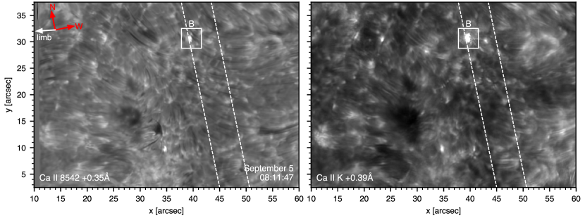
Figure 1: Overview images of the 3 and 5 September, 2016 data sets in the red wing of Ca ii 8542 Å at +0.35 Å (left panels) and Ca ii  K at +0.39 Å (right panels). The location of events selected for further study are highlighted with labelled white boxes in the panels. The slanted dashed lines indicate the extent of the IRIS raster (which extends beyond the upper and lower boundaries of this field-of-view). The red arrows point to Solar North and West, while the white arrows indicate the direction to the closest limb.

2 Observations and data reduction

2.1 Acquisition and data properties

For this study we employ two data sets obtained on September 3 and 5, 2016, respectively. On both days the target was active region NOAA 12585, with the SST pointing at ($X$,$Y$)=($-$561^′′,44^′′) on the 3rd and at ($X$,$Y$)=($-$161^′′,24^′′) on the 5th, corresponding to a viewing angle of $\mu$=0.81 and 0.99, respectively.

At the SST observations were performed with the CRISP and CHROMIS instruments. Both are dual Fabry-Pérot tunable filter instruments, where CRISP has additional polarimetric capabilities. On both days, CRISP provided imaging spectroscopy in the H $\alpha$ line in 15 positions out to $\pm$1.5 Å at 200 mÅ steps and full Stokes imaging spectropolarimetry in the Ca ii 8542 Å line in 21 positions out to $\pm$1.75 Å at 70 mÅ steps in the inner wings and increasing steps of up to 800 mÅ in the outer wings. The cadence of these observations is 20 s. On September 5 this sequence was extended to include full Stokes spectropolarimetry in the Fe i 6301 and 6302 Å lines in 16 wavelength positions, resulting in an overall cadence of 32 s. On both days CHROMIS recorded Ca ii  K and H $\beta$ imaging spectroscopy, but for our analysis we focus only on the former. The Ca ii  K line was sampled out to $\pm$0.7 Å at 78 mÅ spacing and additional samplings at $\pm$1.33 Å as well as a continuum point out at 3999.7 Å. The cadence of the CHROMIS data is 13 s and 12 s for the respective data sets.

On both days these observations were supported by IRIS with a medium dense 16-step raster (OBSID 3625503135). This program covers about 5^′′ $\times$ 60^′′ with continuous 0$\aas@@fstack{\prime\prime}$33 steps at 0.5 s exposure time per slit position, resulting in an overall raster cadence of 20.8 s. As part of the program, the far-UV (FUV) data were spectrally rebinned on-board by 4 to increase the signal-to-noise ratio. Context slit-jaw imaging in the C ii, Si iv, and Mg ii  k bands was recorded at 10.4 s cadence.

Absolute wavelength and intensity calibrations were performed for all data. For CRISP and CHROMIS data the atlas profile by Neckel & Labs (1984) was used, taking into account limb darkening due to the non-vertical viewing angles. For IRIS spectra we followed the standard procedure, with wavelength calibration to the O i 1355.5977 Å line for FUV1 (containing C ii), to Fe ii 1392.817 Å for FUV2 (containing the Si iv lines) and to the Ni i 2799.474 Å line in the near-UV (NUV), while using the wavelength-dependent response functions for the intensity calibration. All resulting intensities are expressed in CGS units as function of frequency (i.e. $I_{\nu}$ [erg s^-1 cm^-2 Hz^-1 sr^-1]).

2.2 Data reduction and alignment

The CRISP data were reduced using the CRISPRED (de la Cruz Rodríguez et al. 2015) processing pipeline, which includes image reconstruction through Multi-Object Multi-Frame Blind Deconvolution (MOMFBD; van Noort et al. 2005). CHROMIS data were reduced using similar procedures, modified from CRISPRED to accomodate for the CHROMIS data format and bundled into the CHROMISRED pipeline (Löfdahl et al. 2018).

The CRISP data were then scaled up to the native CHROMIS pixel scale (from 0$\aas@@fstack{\prime\prime}$0592 to 0$\aas@@fstack{\prime\prime}$0376) and subsequently aligned to the CHROMIS images by iteratively cross-correlating a wavelength-integrated image for every time step in Ca ii  K ($\pm$0.47 Å around the core) with the nearest-neighbour one in time in Ca ii 8542 Å ($\pm$0.45 Å around the core). Similarly, the IRIS to SST alignment was performed using the Mg ii  k slit-jaw images (also scaled up to CHROMIS pixel size), with wavelength-integrated Ca ii images as anchor. After initial guess alignment based on pointing coordinates and FOV rotation, further fine-alignment was achieved through iterative shift and cross-correlation of the images until the correction shift fell below 0.1 (CHROMIS) pixel.

2.3 Event identification and selection

We used the output from an Ellerman bomb detection code EBDETECT (Vissers et al. 2019) as a basis for event selection, as comparison with the intensity images then allows us to identify those Ellerman bombs that also display UV burst signatures. CRISPEX (Vissers & Rouppe van der Voort 2012; Löfdahl et al. 2018) was used for data browsing, event and snapshot selection, as well as verification of the automated detection.

Ideally, we would select events that show both Ellerman bomb and UV burst signatures, as well as events that show only one of those characteristics in isolation, but unfortunately the data at hand only provided examples of the former. Although comparison of the SST and IRIS slit-jaw image fields-of-view indicate a number of events was observed that only had one of the signatures, these were not covered by the IRIS raster. Hence, we selected two events—A and B—for detailed study, observed on September 3 and 5, respectively.

The spectral criterion for an event to classify as a UV burst is to display profiles as described in Young et al. (2018), i.e. substantially enhanced and broadened Si iv lines, although the C ii and Mg ii & k lines are commonly also enhanced. An Ellerman bomb with UV burst signature requires the same IRIS line enhancements in addition to the regular Ellerman bomb signature of bright H $\alpha$ wings and dark core. Both the events under scrutiny have previously been analysed in Rouppe van der Voort et al. (2017).

For both events Ca ii 8542 Å, Ca ii  K and IRIS data are available, while Event B was also covered by additional Fe i spectropolarimetry. The results we present and discuss in the following sections are from inversions of selected snapshots of both events, as well as (temporally downsampled) time sequence of Event A. Before presenting the inversion results, we first discuss the inversion code and setup in the following Section 3.

3 Inversions with the STockholm Inversion Code

We use the MPI-parallel non-LTE STockholm Inversion Code (STiC; de la Cruz Rodríguez et al. 2016, de la Cruz Rodríguez et al. 2019) to invert the SST and IRIS line profiles in order to infer the possible atmospheric conditions. The code builds on an optimised version of RH (Uitenbroek 2001) to solve the atom population densities and in each iteration the pressure scale is computed assuming hydrostatic equilibrium, from which in turn the hydrogen and electron densities are derived using an LTE equation of state (from Piskunov & Valenti 2017). The electron densities can also be derived assuming non-LTE hydrogen ionisation, by iteratively solving the statistical equilibrium equations while imposing charge conservation (similar to Leenaarts et al. 2007). We found, however, that the latter did not significantly change our inversion results (we refer the reader to Appendix A for a results comparison between the two approaches) and therefore decided to assume LTE electron densities instead, with the added benefit of faster and more stable inversions.

The inversions are performed pixel-by-pixel, i.e. assuming 1.5D plane-parallel atmospheres. This means that 3D radiative transfer effects, which are important for Ca ii line cores (Leenaarts et al. 2009, Leenaarts & Carlsson 2009, Leenaarts et al. 2018) and Mg ii lines (Leenaarts et al. 2013a, Leenaarts et al. 2013b, Pereira et al. 2015) cannot be taken into account by the code, however, these should not affect the line wings as much, where the emission of interest is observed. Also for Si iv (which is generally formed under optically thin conditions) this is likely a minor effect. STiC does allow including partial frequency redistribution (PRD) effects by scattered photons (Leenaarts et al. 2012).

We initialise the model atmosphere from FAL-C by interpolating to 44 depth points. While this is unlikely to be close to the solar burst atmospheres that we are interested in, the inversion code already roughly approaches the final results after the first cycle. Modification of the initial atmosphere by moving the transition region to lower heights or by raising the chromospheric temperature plateau did not significantly affect the inversion outcomes.

The inversions are run in multiple cycles, with the general approach being to use fewer nodes in the first cycle to obtain the large scale trends and more nodes in the subsequent cycles to get a more detailed atmospheric structure (as suggested by Ruiz Cobo & del Toro Iniesta 1992). In between the cycles the model atmosphere is smoothed horizontally using a Gaussian with a 2 pixel full-width-at-half-maximum, to decrease the effects of pixels where inversions failed. This smoothing is applied at twice the node resolution, i.e. at every node point as well as at a point equidistantly between each node, followed by interpolation to all other depth points. The smoothed atmosphere is then used as input atmosphere for the subsequent cycle.

While inverting the Ca ii data in isolation (or even with Fe i) is a straightforward and relatively quick process, obtaining reasonable fits when including UV lines is non-trivial as we show in the following. Instead of attempting direct inversion of all available diagnostics, we first perform two cycles with Ca ii (and for September 5 also Fe i) data, using the output atmosphere thereof as input atmosphere for the inversions including IRIS diagnostics.

Table 1 summarises the number of nodes used in each cycle for temperature $T$, line-of-sight velocity $v_{\rm{LOS}}$, microturbulence (or non-thermal velocity) $v_{\rm{micro}}$, the longitudinal and horizontal components of the magnetic field $B_{\rm{lon}}$ and $B_{\rm{hor}}$ (in the frame of the observer, i.e. $B_{\rm{lon}}$ is the line-of-sight component, while $B_{\rm{hor}}$ is that in the plane-of-the-sky), and azimuth $\alpha$. The nodes are by default distributed equidistantly between $\hbox{log $\tau_{500}$}\!=\!0.1$ and $-$8. The exception to this is when we include Fe i, in which case the nodes for $B_{\rm{lon}}$ and $B_{\rm{hor}}$ are placed at specific locations: $\hbox{log $\tau_{500}$}\!=\![-0.5,-2.0,-5.0]$ and $\hbox{log $\tau_{500}$}\!=\![-0.5,-5.0]$, respectively. The third cycle applies only for runs that include IRIS data, i.e. cycles 1 and 2 are run with Ca ii (and if available Fe i) only and the output atmosphere from that second cycle is used as input atmosphere for the third cycle when Mg ii and Si iv are included. In principle, including more diagnostics formed at different heights would warrant increasing the number of velocity nodes, however, tests showed this did not generally yield better fits, hence we retained the number of velocity nodes from the second cycle in those following.

STiC offers four choices in depth interpolation of the parameters: linear, quadratic and cubic Bezier splines (de la Cruz Rodríguez & Piskunov 2013), and discontinuous (Steiner et al. 2016). Tests with single pixels and small patches indicated best results were obtained with linear interpolation when considering only SST data, but that allowing for discontinuities was necessary to better fit Mg ii. When including Si iv best results were again obtained with linear depth interpolation.

The model atoms used for Ca ii, Mg ii and Si iv have 6, 11 and 9 levels, respectively. Ca ii  K and Mg ii & k are computed with PRD, while for Ca ii 8542 Å and Si iv complete frequecy redistribution (CRD) is assumed.

Table 1: Number of nodes used in each inversion cycle.

Parameter	Ca ii 8542 Å		Ca ii (+Fe i)		Ca ii (+Fe i) + IRIS
	1	2	1	2	3A	3B
$T$	4	9	4	9	9	13
$v_{\rm{LOS}}$	1	3	1	4	4	4
$v_{\rm{micro}}$	0	2	1	5	5	5
$B_{\rm{lon}}$	1	2	1	2 (3)a	2 (3)a	2
$B_{\rm{hor}}$	1	2	1	2	2	2
$\alpha$	1	1	1	1	1	1

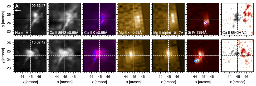
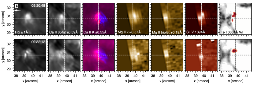
Figure 2: Close-up images of the selected events in the various diagnostics in which they are observed. From left to right: H $\alpha$ summed wings ($\pm$1 Å), Ca ii 8542 Å summed wings ($\pm$0.59 Å), composite Ca ii  K images at the indicated wavelength offsets (with blue wing in blue, red wing in red), Mg ii  k blue wing, Mg ii triplet red wing, Si iv (nominal rest wavelength) and a Stokes $V/I$ magnetogram proxy (from Ca ii 8542 Å for September 3 and Fe i 6301.5 Å at $-$0.07 Å for September 5), with positive and negative polarities in black and red, respectively. For each event—labelled in the top left corner of the H $\alpha$ panel—two snapshots are shown at the times specified in the top right corner of the same panel. The white arrows below the event labels indicate the direction to the closest limb. The dashed cross-hairs do not highlight any particular feature, but are meant to aid in comparing the substructure in various diagnostics. The coloured diamonds in the Si iv panels of Event A (second-to-last panels in the top two rows) indicate locations for which spectra and inversion results are shown in Fig. 12. Panels have been bytescaled individually to better highlight relevant substructure.

4 Results

Figure 2 shows two snapshots of Event A in various diagnostics in its top two rows; the next two rows offer a similar display for Event B. The panels are selected through nearest neighbour interpolation in time with Ca ii  K as leading diagnostic, resulting in a difference of up to 2.9 and 9.2 s between the panels for the two snapshots of Event A and up to 2.3 and 5.3 s for those of Event B. Depending on the frames chosen these timing differences can be much larger, though: for CRISP and CHROMIS the scan-averaged times can differ by nearly 20 s and 6 s for September 3 and 5, respectively, while the offset with IRIS can run up to about 11 s on both days. This can have an appreciable impact on the ability of STiC to obtain agreement between the different diagnostics, in particular for those cases where fast-evolving fine structure is considered (cf. e.g. Felipe et al. (2018), although the effects on the Stokes profiles are not as extreme in our case). The frames displayed here were chosen for their relatively high contrast and the amount of substructure visible in Ca ii  K images.

For Event A H $\alpha$ and Ca ii 8542 Å wing images show much the same morphology, although the Ca ii 8542 Å wing emission is stronger in the top parts of the Ellerman bomb. Comparing the Ca ii 8542 Å and Ca ii  K panels—and as already noted in Rouppe van der Voort et al. (2017)—Ca ii  K reveals additional substructure compared to the CRISP images. Particularly the second snapshot, at 10:02 UT, shows that the more or less monolithic H $\alpha$ and Ca ii 8542 Å brightening at the geometric base of the Ellerman bomb (i.e. crossed by the vertical dashed line at $(x,y)\simeq(45\hbox{${}^{\prime\prime}$},25\hbox{${}^{\prime\prime}$})$) is composed of at least three individual, thin jet-like structures. Striking is also the spatial offset between the location of red and blue K₂ peak emission (third column), where in both snapshots the K_2R enhancement is located at the Ellerman bomb base, while the K_2V enhancement is predominantly observed as the jet tops (cf. the offset between red and blue). Considering the next three panels showing IRIS Mg ii and Si iv this event classifies as an Ellerman bomb with UV burst signature. The fine structure so well-observed with CHROMIS is unsurprisingly lost, but confirms earlier reports (e.g. Vissers et al. 2015) indicating the Mg ii  k wing emission appears co-spatial with the body of the H $\alpha$, while Si iv is offset with respect to the bulk of both H $\alpha$ and Mg ii emission and is mostly observed towards the geometric top of the event. Finally, comparison with the Ca ii 8542 Å Stokes $V/I$ panel suggests opposite polarity reconnection as the driver of this event; guided by the cross-hairs we can readily trace the base of the H $\alpha$ brightenings to the polarity inversion line.

A similar picture emerges for Event B, although geometric effects separating both the bi-directional red- and blue-shifts and the emission at the different IRIS wavelengths are much smaller, as one would expect given the near-vertical viewing angle. Individual jets that can be seen in particularly the second H $\alpha$ snapshot are not that well visible in the Ca ii 8542 Å and Ca ii  K panels, however both Ca ii  K panels show clearly the presence of blob-shaped substructure that the study by Rouppe van der Voort et al. (2017) suggested to be signatures of plasmoids. The Mg ii enhancements overlap largely with the H $\alpha$ and Ca ii emission, while Si iv appears somewhat more offset, however this is difficult to establish conclusively given that the raster does not cover the entire event as observed with the SST. The underlying magnetogram shown in the right-most panels, in this case derived from the blue wing of Fe i 6301.5 Å, again points to opposite polarity reconnection.

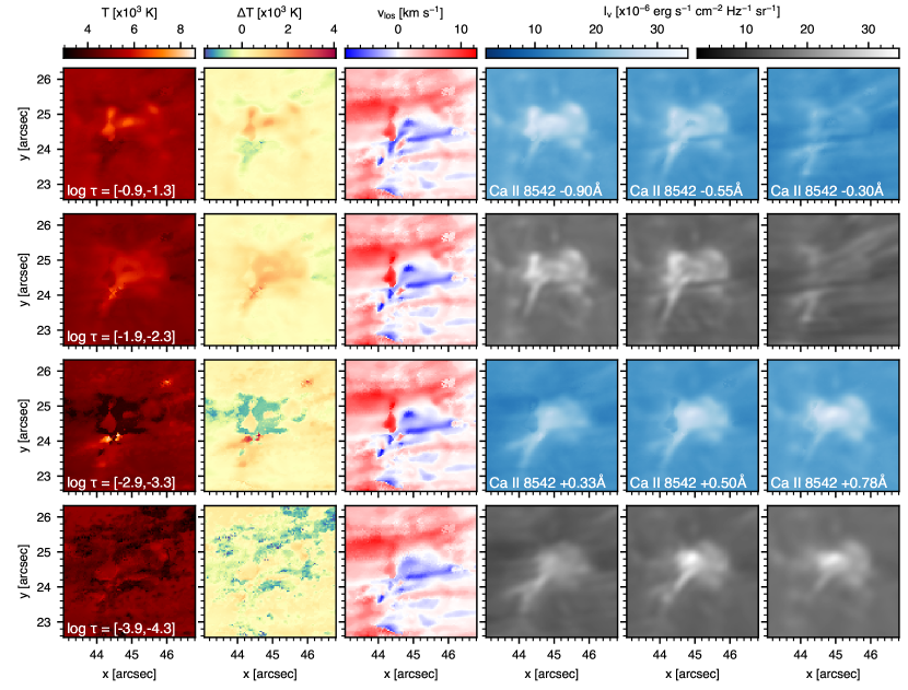
Figure 3: Inversion maps of the second snapshot of Event A (cf. Fig. 2, second row) from the Ca ii 8542 Å-only run at several heights in the model atmosphere (three left-hand columns), as well as synthetic and observed intensity images for comparison (three right-hand columns). From left to right: temperature, the temperature difference with respect to the initial input model, line-of-sight velocity, synthetic (first and third rows) and observed (second and fourth rows) intensity images in the wings of Ca ii 8542 Å, at the wavelength offsets indicated in the synthetic image panels. The log $\tau_{500}$ height for each row is indicated in the lower left of the left-most panels. Panels are scaled by column for the three left-hand columns, while all panels in the three right-hand columns are scaled to the same values, i.e. similar colours in different panels means similar values at different heights or wavelength offsets. The intensity panels have been multiplied by 1.25 to offset absolute intensity differences with Ca ii  K, allowing direct comparison with the Ca ii 8542 Å panels in Figs. 4 and 10.

4.1 Inversions of CRISP and CHROMIS data

We first consider inversions of the CRISP and CHROMIS data of both Events A and B. Figures 3 and 4 show inversion maps of the second snapshot of Event A at four heights in the atmosphere ($\hbox{log $\tau_{500}$}\simeq[-1.1,-2.1,-3.1,-4.1]$, averaged over three nodes around each) from, respectively, the Ca ii 8542 Å-only inversion and the inversion including both the Ca ii 8542 Å and Ca ii  K lines. Figure 6 shows similar maps of the combined Ca ii inversions for both Event B snapshots of Fig. 2.

Event A: Ca ii 8542 Å-only results.

The right-hand columns in Fig. 3 show that the general intensity patterns are well-recovered by the inversion code, including the range of intensity values (the difference in dynamic range between each set of synthetic and observed panels is negligible), although the darker patch to the left of the bright event in the fourth and fifth panels of the third row clearly shows the code has trouble in some parts of the sub-FOV. This feature corresponds morphologically well with the bright event top in the $-$0.90 Å panels (first and second panels in the fourth column), but shows unexpectedly a redshift suggesting the code has difficulties there—likely because of the contribution from the dark fibrils visible in the $-$0.30 Å panels (first and second panels in the last column).

The general shape of the Ellerman bomb is also recovered in the temperature maps at $\hbox{log $\tau_{500}$}\!=\!-$2, albeit with less of the spatial structure than is visible in the intensity panels. At higher heights the event is practically lost, but at $\hbox{log $\tau_{500}$}\!=\!-$1 the compact brightening in the top intensity panels is recovered as an enhanced temperature of some $\Delta T$=1000–2000 K (at $(x,y)\simeq(44\aas@@fstack{\prime\prime}{2},24\aas@@fstack{\prime\prime}{5})$), with a hint of enhanced temperature in a semi-circular arc to the left of the main brightening. Overall the total temperature reaches order 7500–8500 K, corresponding to some $\Delta T$=3000–4500 K over the local ambient temperature. The highest temperatures rise of roughly $\Delta T$=4000 K is found close to $\hbox{log $\tau_{500}$}\!=\!-$3 and its location in the observed plane corresponds to the stronger brightening at $(x,y)\simeq(44\aas@@fstack{\prime\prime}{3},24\aas@@fstack{\prime\prime}{0})$ in the extended jet that is visible both in all intensity panels. The cooler temperatures that cross the event at $\hbox{log $\tau_{500}$}\simeq-$3 and the noisy temperature maps at $\hbox{log $\tau_{500}$}\!=\!-$4 are most likely due to the dark canopy fibrils that are evident in the blue-wing images (in particular those near $-$0.3 Å), but are ill-recovered due to the reduced temperature sensitivity of Ca ii 8542 Å at those heights.

The line-of-sight velocity maps are even more confused. Disregarding the earlier mentioned artefact, there is still a mix of up- and downflows, both at the base of the event (at $(x,y)\simeq(45\aas@@fstack{\prime\prime}{0},24\aas@@fstack{\prime\prime}{5})$) and what would correspond to the jet-like extension towards the lower left. The latter is distinguishable to some extent as a blue-shift protrusion flanked by a small red-shifted feature to its right up to $\hbox{log $\tau_{500}$}\simeq-$3, at $(x,y)\simeq(44\aas@@fstack{\prime\prime}{5},24\aas@@fstack{\prime\prime}{0})$, which also coincides spatially with the location of the largest temperature enhancement.

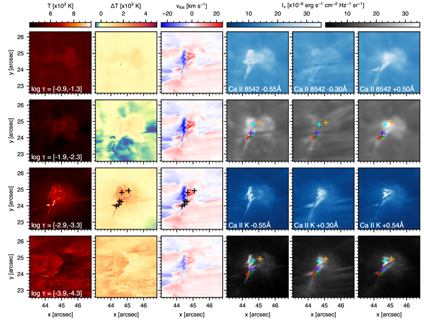
Figure 4: Inversion maps of Event A considering both Ca ii 8542 Å and Ca ii  K. Format as for Fig. 3, except that the right-hand panels in the lower two rows now show the synthetic and observed Ca ii  K intensity images (at the specified wavelength offsets) and those in the upper two rows (i.e. Ca ii 8542 Å) have been multiplied by a factor 1.25 to offset the intrinsic intensity difference between both calcium lines. The coloured plus markers in the right-hand column indicate the locations for which similarly-coloured profiles are shown in Fig. 5. For reference, the same markers are overplotted on the third temperature difference and line-of-sight velocity maps (i.e. around $\hbox{log $\tau_{500}$}\!=\!-3.1$), albeit in black for better visibility.

Event A: Ca ii 8542 Å and Ca ii  K  results.

Comparison with Fig. 4 evidences the advantage of considering multiple diagnostics simultaneously. In particular the panels at $\hbox{log $\tau_{500}$}\simeq-$3 and $-$4 show much better defined structures than with Ca ii 8542 Å alone. In part this is because of the high-resolution CHROMIS Ca ii  K data displaying more fine structure than the CRISP Ca ii 8542 Å images, however, the model is also better constrained by including lines formed at somewhat different heights. The added continuum point from the Ca ii  K observations further constrains the temperature at the lowest heights, resulting in a better fit to the lines and consequently a better constraint of the line-of-sight velocity gradients. Again, the synthetic images in the first and third rows coincide well with the observed ones in the second and third, both in terms of feature shapes and dynamic range, suggesting that also here most profiles are well-fitted.

The top two rows of Fig. 5 highlight this by comparing single-pixel fits to observed profiles for a number of sampling locations in Event A (indicated with identically coloured plus markes in Fig. 4). While the fitted profiles (solid lines) are not perfect everywhere, generally good agreement is obtained for both lines, albeit more so for Ca ii  K than for Ca ii 8542 Å—likely an effect of assigning more weight to the former. Of those shown, the orange and cyan profiles have the largest mismatch issues in one (or both) of the lines, which is likely related to wing asymmetries. For instance, the cyan Ca ii  K profile exhibits a strong blue-over-red asymmetry, which presumably drives the solution to have a similar asymmetry in the 8542 Å line; for the orange profile the absence of such asymmetry in the 8542 Å has lead to underestimate/overestimate the Ca ii  K red/blue wing and K₂ peaks. Another issue may be the time difference (in this case of 8.8 s) between the Ca ii  K and the Ca ii 8542 Å scans, i.e. the observed profiles are not perfectly co-temporal even though STiC assumes they are.

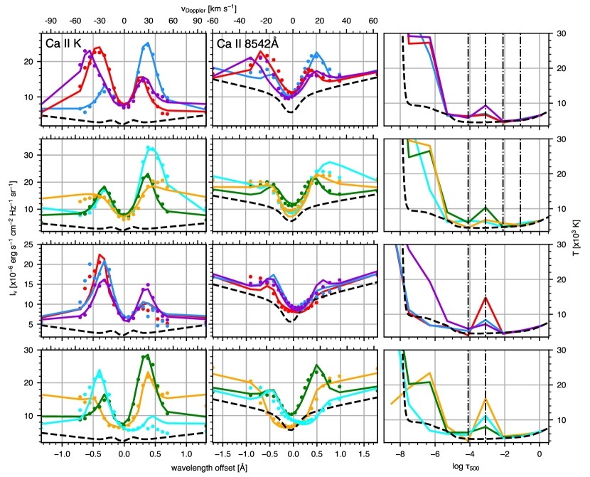
Figure 5: Ca ii  K, Ca ii 8542 Å and temperature profiles for six selected pixels in Events A (top two rows) and B (bottom two rows) at the identically coloured locations marked in Figs. 4 and 6, respectively. The left-hand and middle panels show fits (solid lines) to the observed profiles (filled circles) of the Ca ii  K (left panel) and Ca ii 8542 Å (middle panel) lines, respectively. The corresponding temperature stratification (right-hand panels) is shown using the same colour coding. In the latter, the black dashed curve represents the input temperature stratification (initialised from FAL-C, for which the Ca ii panels show the profiles with similar line style for reference), while the vertical dash-dotted lines indicate the log $\tau_{500}$ heights at which the maps in Figs. 4 and 6 are shown.

While in the Ca ii 8542 Å-only inversion Event A is most clearly visible in the temperature map at $\hbox{log $\tau_{500}$}\!=\!-$2, it is not as clear at that height when combining both calcium lines. At this height, only a narrow zig-zag shaped temperature enhancement that coincides spatially with a brightening of similar morphology in the Ca ii  K blue wing at $-$0.55 Å (third and fourth panels in the fourth column) is evident. Interestingly, this enhanced brightness and temperature coincides with the boundary of the red-shift signature to the right and blue-shifts to the left. On the other hand, the strongest temperature enhancements in the combined Ca ii inversion are reached in similar locations as in the Ca ii 8542 Å-only run. The green and purple crosses mark two of such locations and the corresponding temperature stratifications indicate that some 9500–10,000 K (up to $\Delta T$=5500 K over the ambient input temperature) is reached around $\hbox{log $\tau_{500}$}\!=\!-$3. In addition, for most samplings a sharp temperature increase is found around $\hbox{log $\tau_{500}$}\simeq-$5.5, which for some (e.g. the blue and cyan profiles) represents a considerable lowering of the transition region, while for others (the red, purple, orange and green profiles) it seems to be the increase to a “chromospheric” temperature plateau at some 2.5–3.0 $\times 10^{4}$ K.

Including Ca ii  K has also considerably altered the line-of-sight velocity maps. The extended jet visible in the intensity images is now clearly recovered as an elongated blue-shifted feature of some 15–20 km s^-1 towards the observer, while strong red-shifts of similar magnitude are found at the base of the event. Such bi-directional jet signature was already implied in the composite Ca ii  K image of Fig. 2 (second row, third panel), but is now also confirmed from the inversions.

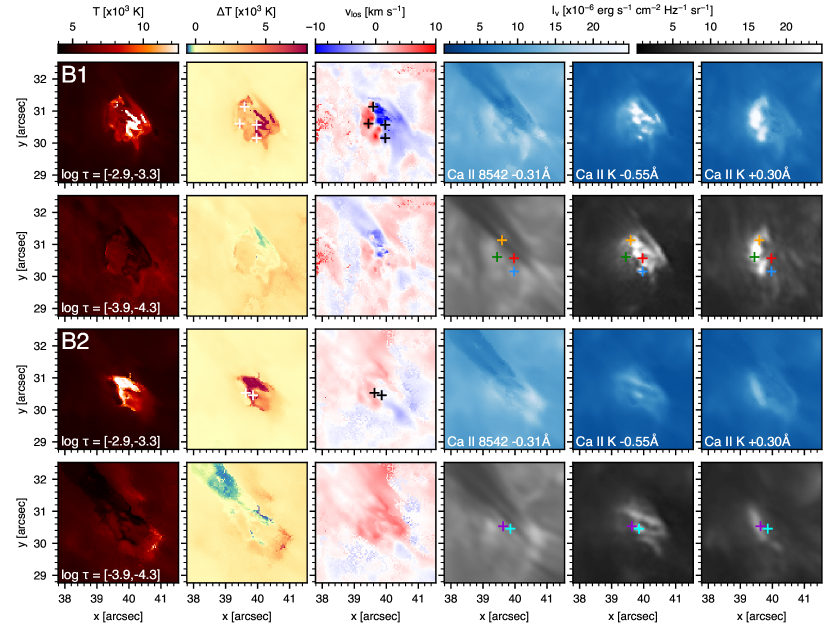
Figure 6: Inversion maps of Event B based on Ca ii 8542 Å, Ca ii  K and Fe i data, in format similar to Fig. 4, but only showing maps at two heights for each Event B1 and B2. The top two rows (B1) show maps for the first snapshot of Event B in Fig. 2; the bottom rows (B2) show those for the second snapshot. The coloured plus signs mark locations for which Ca ii profiles are shown in the bottom two rows of Fig. 5. For the orange location in B1 Fig. 11 also shows Mg ii profile fits.

Event B: Ca ii and Fe i results.

Figure 6 shows the inversion maps for both snapshots of Event B, from including both Ca ii lines and Fe i 6301.5 Å (latter not shown), in similar format as Fig. 4. The upper two rows correspond to the first snapshot (marked B1) and the lower two rows to the second one (B2). Again STiC is able to recover the fine structure in the intensity images (but also the $v_{\rm{LOS}}$ maps), doing slightly better for snapshot B1 than B2, though with very similar results for both Ca ii lines. Overall, for both snapshots the discrepancies are mostly in the Ca ii 8542 Å panels: in case B1 an imprint of the Ca ii  K brightenings is visible that is not there in the observations, while for both B1 and B2 the dark fibrilar structure overlying the event is relatively well-reproduced in intensity at the wavelengths shown. The blob-like substructure is evident for the first snapshot (B1), in particular in the Ca ii  K intensity panels (two right-most panels in the first and second rows). The difference in dynamic range is 1–2$\times 10^{-6}$ erg s^-1 cm^-2 Hz^-1 sr^-1 at most for all panels shown, except the red-wing Ca ii  K images of frame B2 (third panel in the fifth column), where the maximum synthetic intensity falls some 4$\times 10^{-6}$ erg s^-1 cm^-2 Hz^-1 sr^-1 below the observed values. This assessment is supported by the profile fits shown in the lower two rows of Fig. 5, highlighting four pixels from B1 and two from B2. In some cases the large K_2R peak appears to drive a stronger decrease in the Ca ii 8542 Å red wing (e.g. the green profiles) or both lines are overestimated in the wing emission (e.g. red and blue, in particular for Ca ii  K); in others (e.g. purple and orange) both lines are well-fitted simultaneously.

The velocity maps for both frames B1 and B2 do not show as clear a spatially resolved bi-directional jet structure as for Event A. Rather, the majority of blobs in B1 show either a clear red-shift/blue-shift of order 10–12 km s^-1 away/towards the observer. The line-of-sight velocities are strongest around the height where the temperature peaks, $\hbox{log $\tau_{500}$}\!=\!-$3. The dark fibrils seen in the blue wing of Ca ii 8542 Å are well-recovered in the synthetic intensity images and the $\hbox{log $\tau_{500}$}\!=\!-$4 panel for Event B1 (third panel in the second row) displays a moderate blue-shift with similar morphology at that same location.

In terms of temperatures, the inversions suggest even higher values are reached in Event B than for Event A. Both snapshots B1 and B2 show hot patches of up to 15,000 K total temperature, peaking between $\hbox{log $\tau_{500}$}\!=\!-2$ and $-$4 (cf. Fig. 5), and while one would be hard-pressed to recognise the blob-like morphology from these temperature maps, the largest temperature enhancements are found at the locations where the brightest blobs are visible in the Ca ii  K images. The temperature stratification shown in the last panel of the lower two rows of Fig. 5 is similar to that for Event A: a temperature increase around $\hbox{log $\tau_{500}$}\!=\!-$3 and a rise to the transition region or enhanced chromospheric plateau close to $\hbox{log $\tau_{500}$}\!=\!-$5, even though for half of the samplings the transition region rise lies close to that of the input model. The apparent decrease above $\hbox{log $\tau_{500}$}\!=\!-$7 for the orange sampling is an effect of extrapolation beyond the last node with the slope at the last node.

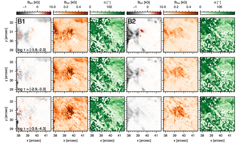
Figure 7: Inversion maps of magnetic field quantities for both Event B snapshots. From left to right: line-of-sight magnetic field strength (with positive/negative (i.e. red/black) corresponding to field oriented towards/away from the observer), horizontal magnetic field strength and azimuth for Event B1, followed by similar maps for B2. As only one node was used in azimuth, the corresponding maps are identical for the three heights shown. The panels have been scaled by column to the same values for both B1 and B2 to facilitate comparison of the time evolution between them.

4.2 Magnetic fields

As for Event A only Ca ii 8542 Å polarimetry was available, we allowed fewer degrees of freedom and the inverted field was consequently not well-defined with height. However, with the availability of Fe i for Event B we added a third node in line-of-sight magnetic field strength and obtained more reasonable results. Figure 7 shows the magnetic field inversion maps at the same log $\tau_{500}$ heights as Fig. 6 shows the other inversion parameters, as well as around $\hbox{log $\tau_{500}$}\!=\!-$1. While obviously noisy, clear signal is obtained for the longitudinal and horizontal magnetic fields. As only one node was used to fit the azimuth, the maps look the same at all shown heights.

Especially at the lowest heights the photospheric magnetic field pattern visible in Fe i Stokes $V/I$ (right-hand panels in the lower two rows of Fig. 2) is also clearly recovered in the $B_{\rm{lon}}$ panels. Going to higher heights the signal gets weaker and more homogenous, as one would expect from the expansion of the field. The horizontal magnetic field strength maps are largely devoid of signal and generally noisy, yet do show enhanced signal at the location where the brightenings are visible at $\hbox{log $\tau_{500}$}\!=\!-$3 and $-$4. For B1 this enhanced horizontal field interestingly overlaps with the location where the $v_{\rm{LOS}}$ signature flips sign in the top row of Fig. 6. The azimuth maps are noisy at best and do not show a clearly defined structure coinciding with the event brightening, temperature or line-of-sight velocity structures, although the values are typically low (below about 40^∘) and spatially smoother at the locations of enhanced $B_{\rm{hor}}$. Considering the changes with time going from B1 to B2 we observe an increase of the longitudinal magnetic field, mostly at the lower heights i.e. $\hbox{log $\tau_{500}$}\!=\!-$2 and $-$3, while the horizontal fields at the location of the event decrease by nearly 500 G (the maximum $B_{\rm{hor}}$ values are slightly over 1.1 kG for B1). In addition, the B2 maps for $B_{\rm{lon}}$ at $\hbox{log $\tau_{500}$}\!=\!-$2 (displaying clear opposite polarity footpoints) and $B_{\rm{hor}}$ at $\hbox{log $\tau_{500}$}\!=\!-$4 (with enhanced horizontal fields) are consistent with with a $\cap$-configuration or possibly the shared horizontal part of a post-reconnection $\cap$- below $\cup$-configuration.

Figure 8: Time sequence of inversion maps of Event A from combining Ca ii 8542 Å and Ca ii  K. From left to right the columns show temperature (left-most three columns), the temperature difference with the input model (middle three columns) and line-of-sight velocity (right-most three columns) at the log $\tau_{500}$ heights specified in the first row panels. The time in UT is indicated in the top left of the first panel of each row. The panels have been bytescaled by column (ranges indicated by the colour bars at the top of each column). The dashed lines in rows 5, 8 and 9 indicate the lines along which Fig. 9 shows cross-cut inversion maps.

4.3 Time evolution

Let us now consider the time evolution of Event A. Figure 8 shows the top-down inversion maps based on Ca ii 8542 Å and Ca ii  Kfor temperature, temperature difference and line-of-sight velocity for this event as function of time at roughly 50 s intervals. Throughout this sequence the event stands out in the temperature maps as an enhancement of a few thousand kelvin up to a total temperature of 8000–10,000 K, in particular around $\hbox{log $\tau_{500}$}\!=\!-$3. At $\hbox{log $\tau_{500}$}\!=\!-$2 and $-$3 it is clearly hotter than its surroundings, while at $\hbox{log $\tau_{500}$}\!=\!-$4 the whole sub-field-of-view appears enhanced in temperature by $\Delta T$=2000–2500 K and the event starts to blend in.

The bi-directional jet signature so clearly visible in the middle column of Fig. 4 (and second-to-last row of this figure, at 10:02:42 UT) can be observed at several stages during the time evolution, although a line-of-sight blue-shift of up to $-$25 km s^-1 appears to be the persistent velocity signature. In addition, both the top few rows (09:56:41–09:58:25 UT) and bottom few ones (10:01:51–10:03:34 UT) appear to show the blue-shift velocity imprint from overlying canopy fibrils to the left of the event. Similar to some of its preceding frames (not shown here), the top row shows red-shift artefacts embedded in otherwise smooth blue-shifts in the $v_{\rm{LOS}}$ maps or enhanced and decreased temperatures at $\hbox{log $\tau_{500}$}\!=\!-$2 and $-$3, respectively, which corresponds to locations where the maps suffer from worse line fits.

Figure 9: Cross-cut inversion maps of Event A from selected time steps highlighted in Fig. 8. From left to right: $x$-log $\tau_{500}$ cut in temperature, temperature difference and line-of-sight velocity, followed by the $y$-log $\tau_{500}$ cuts in the same quantities. The panels have been scaled by column, where the quantities have been clipped to the respective colour bar values. The vertical markers in the $x$-log $\tau_{500}$ ($y$-log $\tau_{500}$) panels indicate the location where they are intersected by the $y$-log $\tau_{500}$ ($x$-log $\tau_{500}$) cut. The lower row displays the cross-cuts of the same frame as in the third row, but now from the inversions including Mg ii.

Figure 9 shows cross-sectional inversion maps for three selected frames from the time sequence in Fig. 8 along the lines indicated in the respective panels; the third and fourth rows of maps correspond to the second Event A snapshot of Fig. 2, where the fourth row is from the inversions including Mg ii. As was already implied by the temperature maps in Fig. 8 and the temperature profiles in Fig. 5, the temperature enhancements related to the Ellerman bomb/UV burst are generally located between $\hbox{log $\tau_{500}$}\!=\!-$2 and $-$4, peaking around $\hbox{log $\tau_{500}$}\!=\!-$3. As indicated before, between $\hbox{log $\tau_{500}$}\!=\!-$5 and $-$6 we find a sharp temperature increase to an enhanced chromospheric plateau or due to the actual transition region overlying the event coming down compared to the FAL-C input (where it lies close to $\hbox{log $\tau_{500}$}\!=\!-$8).

The line-of-sight velocity cross-cuts suggest bi-directional flows with the expected red-shifts below blue-shifts within some of the pixels (cf. e.g. the $x$-log $\tau_{500}$ cuts for all three frames or the $y$-log $\tau_{500}$ for the top two). Interpreting these as the bi-directional reconnection jet within the pixel (i.e. within the $x$-log $\tau_{500}$ or $y$-log $\tau_{500}$ column) would, however, imply the reconnection takes place above the main temperature increase, as the $v_{\rm{LOS}}$ divergence point is located around $\hbox{log $\tau_{500}$}\!=\!-$5 in these examples. Given that the bi-directional signature is clearly separated spatially in the top-down view, one could imagine the blue-shift should be observed in adjacent pixels rather than in the same (i.e. to the top left in these $x$-log $\tau_{500}$ cuts). This is the case for all three examples shown, but the extension of both signatures over $\hbox{log $\tau_{500}$}\!=\![0,-4]$ is somewhat puzzling, i.e. even though opposite signatures in adjacent pixels is expected, we would also expect the blue-shifts to be found predominantly at comparatively higher heights than the red-shifts. To some extent this is the case in the $x$-log $\tau_{500}$ $v_{\rm{LOS}}$ panel of the first frame (top row, third panel), where a blue-shift can be found to the top left (around $\hbox{log $\tau_{500}$}\!=\!-$4.5) of the stronger red-shift, although this again places the outflow point above the main heating location. The same cut for the next two frames shows this much less clearly (if at all); the blue-shifts left of the red-shifts extend only marginally higher than the red-shifts. An issue that could play a role here is the limited number of $v_{\rm{LOS}}$ nodes used in the inversions, thereby preventing STiC from finding a consistent solution that places the outflow point lower down. Increasing the number of nodes may have alleviated this, however, as pointed out previously increasing the number generally resulted in worse fits to the Ca ii lines, hence our choice not to do so. The fourth row, from inversions including Mg ii, is further discussed in the following section, but we note here that the general temperature and velocity patterns are largely the same between the inversions with and without that Mg ii lines.

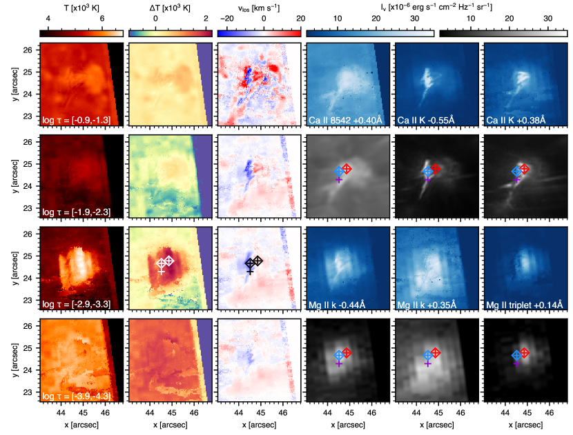
Figure 10: Inversion maps of Event A considering both Ca ii lines and Mg ii & k. Format as for Fig. 4, except that the six panels in the lower right now show (from left to right) an image of the Mg ii k_2V, k_2R and the red wing of the subordinate Mg ii triplet. The Ca ii 8542 Å, Mg ii  k and Mg ii triplet images have been multiplied by 1.25, 7.5 and 10, respectively, to roughly offset the intrinsic intensity difference with the Ca ii  K line and all panels in the three right-hand columns have been scaled to the same values subsequently (these are the same values as in Figs. 3 and 4). The triangular area to the (upper) right of the inversion maps has values set to zero as these fall outside the IRIS raster. The coloured plus markers in the second and fourth rows mark the locations for which profiles are shown in the top two rows of Fig. 11; the coloured diamond markers those locations for which Fig. 12 shows profile fits including Si iv. The purple cross marks the same location as the purple cross in Fig. 4.

4.4 Inversions of combined SST and IRIS data

We have seen earlier that including additional diagnostics generally constrains the model atmospheres better and given that Mg ii & k are typically formed somewhat higher than Ca ii (cf. e.g. Fig. 1 from Leenaarts et al. (2013b) or Fig. 15 from Bjørgen et al. (2018)), this should help the inversions. Moreover, finding an atmospheric model that can explain also the UV part of an Ellerman bomb is of great interest.

When including IRIS the instrumental resolution differences are, however, non-negligible and a likely source of errors: already between CRISP Ca ii 8542 Å and CHROMIS Ca ii  K there is a factor 2 difference in resolution, going up to over a factor 8 when comparing CHROMIS and these IRIS raster observations. As we chose not to sacrifice resolution, the IRIS profiles have been interpolated to the CHROMIS pixel scale, i.e. a single IRIS spectral profile is spread out over many SST pixels. Consequently, STiC considers these one-to-one, while in reality many SST profiles should be contributing to the atmosphere that explains the single IRIS profile. Without a well-defined spatial point spread function for either the SST or the IRIS spectrograph it is impossible for STiC to take the resolution difference into proper account.

Also, as with the previous inversions, additional uncertainty arises from the acquisition time difference between the different instruments. On both days the time difference with IRIS can be as large as nearly 11 s. While this effect can be minimised, it may still play an important role, particularly when considering the fast evolution of the Ca ii  K substructure where some plasmoid blobs are sometimes only visible for a single frame.

Notwithstanding these issues, the solution to which inversions converge is not significantly different from the runs without Mg ii, as we show below.

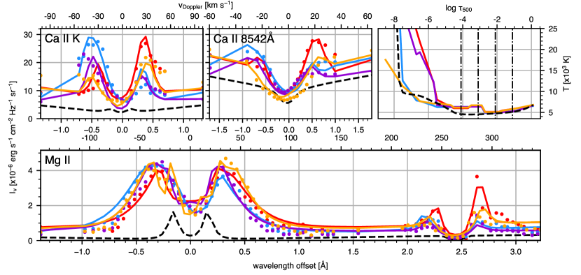
Figure 11: Ca ii  K, Ca ii 8542 Å, Mg ii and temperature profiles for selected pixels in event A (red, blue and purple) and Event B (orange) at the similarly-coloured locations marked in the right-hand panels of Figs. 10 and 6, respectively. Format simlar as for Fig. 5, except that the second row now shows the Mg ii  k and Mg ii triplet lines (the zoom-in has been chosen such to allow easier comparison of the observed and inverted profiles, omitting Mg ii  h because it behaves similarly to Mg ii  k). The input observed Mg ii profiles are shown with every other point to avoid cluttering the plot.

4.4.1 Combining Ca ii and Mg ii

Figure 10 presents in similar format as before the inversion results from including Mg ii along with the Ca ii lines for Event A. Comparing Figs. 4 and 10 for Event A we see that at lower heights ($\hbox{log $\tau_{500}$}\!=\!-$1 and $-$2) the temperature maps look very similar between the runs without and with Mg ii (a hint of the fine structure imprint from Ca ii  K remains visible in the Mg ii results). In fact, at both heights the range of temperatures is similar between the runs and also the average temperatures fall within 50–250 K of each other. Also for both, the line-of-sight velocity maps show clearly the bi-directional jet in most panels of the middle column, most clearly so at $\hbox{log $\tau_{500}$}\!=\!-$2. However, when including Mg ii the bi-directional pattern is much more noisy at $\hbox{log $\tau_{500}$}\!=\!-$1.

The differences are more pronounced higher up. On one hand, the contribution from the IRIS-observed Mg ii is evident in the temperature maps around $\hbox{log $\tau_{500}$}\!=\!-$3 through a more dispersed temperature enhancement, devoid of much of the substructure that was visible when considering only SST data. At $\hbox{log $\tau_{500}$}\!=\!-$4 the event nearly blends into the background in the temperature maps, with the whole sub-FOV displaying a more or less homogeneous temperature enhancement of roughly $\Delta T$=2000 K over the input temperature. Also, while in the Ca ii run the bi-directional velocity signature remains clearly visible throughout the inverted atmosphere, when including Mg ii this signature is more pronounced in the sense that the redshifts are stronger at lower heights, likely due to the contribution from the Mg ii triplet (cf. the lower right intensity panels), and disappear almost entirely at $\hbox{log $\tau_{500}$}\!=\!-$4. This is also reflected in the line-of-sight velocity cross-cut pattern differences between the third and fourth rows of Fig. 9, the latter from inversions including Mg ii. For instance, the strong red-shifts in the $x-\hbox{log $\tau_{500}$}$ cut (third panel of the third row) do not extend as high when including Mg ii (fourth row) and in the latter the adjacent blue-shift (at $x\simeq 44\aas@@fstack{\prime\prime}{2}$) is also largely concentrated between $\hbox{log $\tau_{500}$}\!=\!-$2 and $-$4, rather than extending all the way from log $\tau_{500}$​=​0 to $-$4. This fits with the expectation that the blue-shifts should be found at comparatively higher heights than the red-shifts.

Figure 11 shows the Ca ii and Mg ii fits with corresponding temperature profiles for identically coloured selected pixels in Figs. 10 (red, blue and purple; Event A) and 6 (orange; Event B). The fits are generally good, although getting agreement in these three lines simultaneously is more challenging than for the two Ca ii lines alone. For the examples from Event A, the profile asymmetries are strongest in Ca ii  K and the brighter K₂ peak is also typically the one that is better fitted (cf. e.g. the red and blue profiles), while the K₃ core is sometimes too dark (e.g. purple and orange profiles), and in some cases the line wings are not bright enough (orange profile). By comparison, the fits to Ca ii 8542 Å show generally fewer discrepancies with the observations than Ca ii  K(except for the orange sampling). As before, it is however possible that differences in the magnitude of the asymmetries between these lines may affect the fitting of one of the line wings. For Mg ii  k the k₂ peaks and inner wings are typically well-fitted, while showing more (though still minor) issues in the k₃ core and further out in the wings, beyond $\pm$0.75 Å, the latter being usually too bright compared to the observations. The Mg ii triplet and its asymmetries are also generally well-reproduced.

Considering the temperature stratification, the peak temperatures of order 1–1.5$\times$10⁴ K that resulted from the Ca ii inversions are interestingly not found when including Mg ii. Rather the temperature enhancement is a moderate $\Delta T$=2500 K over the ambient temperature at $\hbox{log $\tau_{500}$}\!=\!-$3 and for both events the stratification shows an extendend plateau over a range of $\Delta\hbox{log $\tau_{500}$}\simeq\ 2.5$ upward from there. This is also evident from the temperature cross-cuts (cf. the lower row of Fig. 9). In particular the purple profile for Event A (or the orange one for Event B), corresponding to the same sampling location for which the purple (orange) profile in the first (fourth) row of Fig. 5 is shown, now only reaches a total temperature of some 6500 K. We discuss these differences further in Section 5, but note already here that this is likely an effect of the pixel size difference between the IRIS and SST data.

4.4.2 Challanges posed by Si iv

As defined in Young et al. (2018), the primary identification of UVBs is through their enhanced and broadened Si iv lines and properly reproducing this diagnostic is therefore important for a complete description of these events. Unfortunately, at this point this is easier said than done and after several tests we decided to refrain from inverting maps including the Si iv lines.

Figure 12 evidences why. This figure shows the profile fitting results of single pixel inversions at the locations marked with diamonds in the top rows of Fig. 2 (two of which are also overplotted in Fig. 10). Apart from the Ca ii and Mg ii lines as shown before, a fourth spectral panel now displays the Si iv lines with the 1394 Å (1403 Å) observations and fits as dots and solid lines (plus markers and dashed lines), respectively. The Si iv 1402 Å profiles have been multiplied by 2 to account for the offset between the two Si iv lines when formed under optically thin conditions: comparison of the dots and plus markers for each sampling line pair indeed suggests they likely are, as the Si iv 1394 Å to 1403 Å ratio is close to 2 for the purple and blue samplings, while the red one is clearly non-thin given a line ratio of 1.7.

The samplings shown were selected to test fitting of Si iv profiles with varying degrees of complexity (blue-asymmetry for both blue and red samplings versus more ragged-top purple sampling profiles). While STiC may be able to reproduce the general broadening, enhancement and asymmetry of the Si iv lines, this results in completely off profile fits for Mg ii in particular. Of both Si iv lines, the 1403 Å line (plus markers and dashed lines) is sometimes considerably better fitted, e.g. the red sampling. Even though not being perfect, the red-shift side “plateau” mimicks the observations better for 1403 Å than the solid line follows the 1394 Å dots. This further supports the non-thin formation already implied by the line ratio departure from 2. For the blue sampling both lines are fitted equally bad, in the sense that the hump on the red-shift side is not fitted at all, but the fit retains a rather Gaussian shape while recovering the peak intensity. In contrast, the purple sampling shows the best fits for both lines of these three examples, even though it does not fully reproduce the observed intensities between about $-$50 km s^-1 and the nominal line centre.

The temperature profiles (top right panel, solid coloured lines) do show some changes with respect to the inversion results when only SST diagnostics were considered (dashed coloured lines). The temperature peaks that after cycle 2 were already there close to the input temperature minimum (e.g. blue and red) get shifted to lower heights by about $\hbox{log $\tau_{500}$}\!=\!0.5$, while also increasing by a few thousand kelvin. For the purple sampling the temperature enhancement close to the temperature minimum was less pronounced when considering only SST data, but gets a noticeable peak now just below $\hbox{log $\tau_{500}$}\!=\!-$3 when including both Mg ii and Si iv.

The behaviour at higher heights is also changed. For instance, where the red and purple samplings previously showed an increase to a chromospheric plateau of about 3 $\times 10^{4}$ K and 2.5 $\times 10^{4}$ K, respectively, the red temperature profile now shoots up to a plateau over 3.5 $\times 10^{4}$ K and the purple profile shows a pronounced peak up to 4.3 $\times 10^{4}$ K at $\hbox{log $\tau_{500}$}\simeq\,-6.3$. The blue sampling does not show such enhanced temperature between $\hbox{log $\tau_{500}$}\!=\!-$7 and $-$6, but the transition region temperature rise starts about $\hbox{log $\tau_{500}$}\!=\!0.5$ lower when including both Mg ii and Si iv. It should be noted, however, that the inversions with Si iv were run with 13 nodes in temperature, two more than the second cycle inversions, which may explain both the slight shift of the low temperature peaks (since the nodes are slightly shifted), and the ability to resolve the pronounced temperature peak at $\hbox{log $\tau_{500}$}\simeq\,-6.3$ for the purple sampling (considering that the purple dashed temperature profile already showed a high temperature chromospheric plateau).

All in all, while both Ca ii lines are also well-fitted for all three samplings (and better so than Si iv), it is clear that in general agreement cannot be reached for all diagnostics simultaneously with the proposed node models (Mg ii being the most difficult to reconcile). Considering the temperature profiles this is likely due to the temperature peaks to some 10⁴ K between $\hbox{log $\tau_{500}$}\!=\!-$3 and $-$4, which (as shown in the first part of this section) were suppressed when considering Ca ii and Mg ii together. Other issues that may play a role include the limitation to pixel-by-pixel atmospheres (i.e. restriction to 1.5D), the difference in data resolution, non-zero acquisition time differences for the spectra and the limited number and/or placement of temperature inversion nodes. We discuss these further in Section 5, but address the latter shortly here.

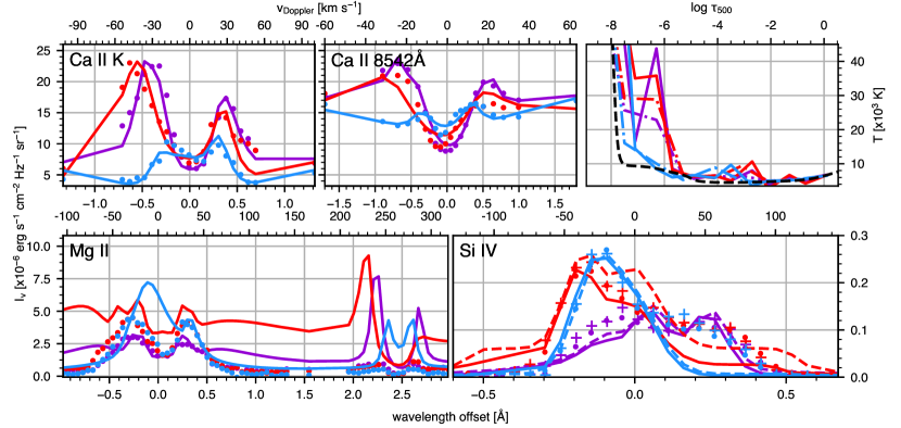
Figure 12: Observed and inverted Ca ii 8542 Å, Ca ii  K, Mg ii, Si iv profiles, as well as the corresponding temperature stratification, for selected pixels in Event A (highlighted with diamond markers in Fig. 10 for the red and blue profiles; the purple profiles corresponds a pixel in the middle of the Si iv brightening in the earlier Event A snapshot shown in the top row of Fig. 2). Format similar to Fig. 11, except that the lower row contains an additional panel with the Si iv 1394 Å (1403 Å) line, where the observed profiles are shown as dots (plus markers) and the fits as solid (dashed) lines. The observational and synthetic Si iv 1403 Å data have been multiplied by 2 to offset the intrinsic intensity difference with 1394 Å under optically thin conditions. The temperature profile panel also includes dash-dotted lines for each sampling indicating the result from the previous inversion cycle (i.e. SST data only).

4.4.3 Effects of sharp temperature enhancements

Certain temperatures need to be reached in order to yield any measurable intensity increase in Si iv, but because of the node distribution such temperature bump will typically be broad in log $\tau_{500}$ corresponding to significant heating over a large height range. This is probably one of the reasons for the overestimated enhancement of Mg ii seen in Fig. 12. Considering the observation of plasmoid-like blobs and indications from numerical studies (e.g. Ni et al. 2018a; Ni et al. 2018b) that in some configurations the plasmoids may have associated confined slow- and fast-mode shocks reaching sufficiently high temperatures to explain Si iv emission, it may be that this emission is very localised and hence impossible to resolve with the current node representation.

As a first step towards further investigating this possibility, we forward-modeled the emergent intensity in Si iv, Mg ii and Ca ii assuming a sharp temperature enhancement at specific heights, sharper than our inversion node placement would allow to recover. We tested a grid of temperatures (at $\Delta T=2500\,K$), peak locations (at $\Delta\hbox{log $\tau_{500}$}\!=\!0.2$) and base widths ($\hbox{log $\tau_{500}$}\!=\!0.05$, 0.1, 0.2 and 0.3), but here only show a sub-selection to highlight certain effects of varying these three parameters. Figure 13 presents the results of this spectral synthesis for several examples of single temperature spikes on top of the inverted temperature profiles based on Ca ii and Mg ii data that produce Si iv emission within an order of magnitude of the observed profile in terms of peak intensity, where the top (bottom) subfigure shows the effect of localised temperature enhancements between $\hbox{log $\tau_{500}$}\!=\!-$5.9 and $-$4.9 ($-$4.1 and $-$3.1). It is clear that regardless of the input temperature profile, the broadening of the Si iv is not well-reproduced, yet this is not surprising: for one, the velocity components (both line-of-sight and non-thermal) were not modified from the preceding inversion output, but more importantly, in optically thin formation the width is only influenced by microturbulence and velocity gradients over the formation region and since the latter is purposefully narrow, the profile width will be relatively small as well.

Considering the higher altitude perturbations (i.e. top subfigure) first, adding the shown temperature spikes does not considerably change the Ca ii or Mg ii profiles, except the k₃ core of the latter when the spike is located below about $\hbox{log $\tau_{500}$}\!=\!-$5.5 (orange-red and purple profiles). Comparing identically coloured temperature and Si iv profiles, we see that an increased base width at the same height and peak temperature (e.g. full and dark red, as well as all three purple profiles) causes an increased Si iv peak intensity. This is to be expected as the volume that is exposed to the heating is larger, thus resulting in a stronger Si iv emission. At the same time this does not appear to affect its line width, i.e. the full-width-at-half-maximum remains essentially unchanged.

The low-altitude perturbations (bottom subfigure) have an effect on all lines, but most conspicuously on the Ca ii 8542 Å core, Mg ii peaks and wings and the Si iv line. Ca ii  K shows similar profiles regardless of the temperature spike location, height and width, although the K₃ core is darker for the lower location temperature spikes and the K₂ peaks are more enhanced for the higher located spikes. The higher location spikes (i.e. close to $\hbox{log $\tau_{500}$}\!=\!-$4) affect both the Ca ii 8542 Å core—which is considerably enhanced compared to the observations—and the Mg ii  k and Mg ii triplet peaks. On the other hand, the lower location temperature spikes (purple profiles) show a larger influence on the (quasi-)continua outside the Mg ii and Si iv lines, overestimating their intensity, sometimes by more than an order of magnitude.

As one would expect, at higher heights one generally requires higher temperatures than at lower heights to get similar Si iv emission, but in either case similar profiles can be obtained from either a narrow but tall or a broader but lower temperature spike. The narrowest of temperature spikes can indeed reproduce specific Si iv intensities at (or close to) the nominal line core, but better profile correspondence likely requires modifying other parameters, such as the line-of-sight velocity. In addition, the temperature spikes at lower heights pose problems for the Mg ii emission in particular, but depending on the height also for the Ca ii 8542 Å core intensity; this may explain why the inversions favoured a solution where the temperatures were enhanced closer to $\hbox{log $\tau_{500}$}\!=\!-$6, rather than around the heights where Ca ii inversions suggested the temperature increase to be. Hence, it is clear that this requires further study, yet as this likely requires a different approach we defer further investigation into the UV burst Si iv line formation to a future study.

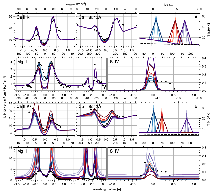
Figure 13: Spectral synthesis of Ca ii, Mg ii and Si iv based on modified inversion atmospheres of two well-fitted pixels of Event A. Temperature peaks have been added at three log $\tau_{500}$ heights (differentiated by colour) with various peak heights and base widths (differentiated by colour shades, increasingly darker for increasing width and/or decreasing peak height). Subfigure A (top two rows) shows the results for placing such enhancement of log $\tau_{500}$-width 0.1–0.3 (from light to dark shade) somewhere between $\hbox{log $\tau_{500}$}\!=\!-$5.9 and $-$4.9. Subfigure B (bottom two rows) offers a similar display for spikes of log $\tau_{500}$-width 0.05, 0.1 and 0.3 (from light to dark) at heights between $\hbox{log $\tau_{500}$}\!=\!-$4.1 and $-$3.1. The underlying observations are from different pixels for the two subfigures. Each subfigure has similar format as Fig. 12, with the spectral panels showing the observations as black dotted profiles and synthesis output as coloured solid lines.

5 Discussion

5.1 Temperature stratification

The observation of Si iv and C ii emission sometimes correlated and co-spatial with typical H $\alpha$-observed Ellerman bombs has added an additional layer of complexity requiring explanation and also led to a heated debate over the past few years on the temperatures these events may reach. Prior to the IRIS launch, Ellerman bomb temperature estimates ranged anywhere between a few hundred to a few thousand kelvin over the ambient temperature at close to temperature minimum heights, generally based on 1D semi-empirical modelling (Kitai 1983; Berlicki et al. 2010; Bello González et al. 2013; Berlicki & Heinzel 2014) or two-cloud modelling (Hong et al. 2014). On the other hand, Socas-Navarro et al. (2006) obtained temperatures of 1–1.2 $\times 10^{4}$ K between roughly $\hbox{log $\tau_{500}$}\!=\!-$3.5 and $-$5 from inversions of the Ca ii 8498 Å  and 8542 Å lines using a predecessor of the inversion code NICOLE. A recent study by Libbrecht et al. (2017), considering He i  D₃ and 10830 Å, suggests temperatures of order 15,000 K would be consistent with their observations. Profile fitting efforts by Grubecka et al. (2016) were able to reproduce the observed IRIS Mg ii  h profiles with temperature enhancements of $\Delta T$=1100–3350 K (up to roughly 8000 K total temperature), while also yielding Ellerman bomb-like H $\alpha$ profiles.

More recently, Reid et al. (2017) and Hong et al. (2017) used the radiative hydrodynamics code RADYN to model Ellerman bombs and found that temperature enhancements of up to $\Delta T$=3000 K yielded H $\alpha$ and Ca ii 8542 Å profiles similar to observations. Both studies also considered Mg ii  k, where a larger energy deposition was required to obtain profile shapes similar to the observations, however, simultaneous agreement between all three diagnostics could not be achieved in either of those studies. They also noted—as did Fang et al. (2017)—that temperatures in excess of 10,000 K caused the computed H $\alpha$, Ca ii 8542 Å and continuum emission to be overestimated compared to observations.

Our results largely agree with these previous findings, yet with some notable exceptions. As shown in the temperature maps (e.g. Figs. 4, 6 or 8), combined Ca ii 8542 Å and Ca ii  K inversions yield total temperatures of some 7000–9000 K close to the temperature minimum throughout most of the events, however, localised temperatures of 1.5 $\times 10^{4}$ K are found as well. The highest temperatures are typically associated with the blue-shifted parts of the events (cf. e.g. the second and third panels of the third row in Fig. 4 or in the first row of Fig. 6). Another difference with previous studies is the occurrence of marked temperature plateaus at 2–3 $\times 10^{4}$ K above $\hbox{log $\tau_{500}$}\!=\!-6$ for some pixels (e.g. purple and red samplings in the top row of Fig. 5 or the green sampling in the bottom row of the same figure). However, the sensitivity of the Ca ii (and Mg ii) lines is very limited above $\hbox{log $\tau_{500}$}\simeq-6$ (cf. also the response functions to temperature in appendix Fig. 17) and while in some cases the line cores may sense (and thus require) the lower part of this temperature rise around $\hbox{log $\tau_{500}$}\simeq-$5.5, the presence or absence of the higher-located plateaus should not be overinterpreted. The case is clearly different when considering Si iv, as both Figs. 12 and 13 suggest that temperature modifications at these heights may have an appreciable effect on the Si iv line intensity.

A notable effect of taking Mg ii & k into consideration is that the peak temperatures around $\hbox{log $\tau_{500}$}\!=\!-3$ are reduced compared to the Ca ii inversion results. Intuitively, as Mg ii is formed higher than either of the Ca ii lines, one would expect higher temperatures to be recovered when including the Mg ii & k lines (or at the very least not as strong a reduction as we find). However, this is likely not a physical effect, but rather because of the difference in resolution between SST/CHROMIS and IRIS (and possibly timing differences as well), as pointed out previously in Section 4.4.1 and discussed in Section 5.5.

Both the selected pixel examples (Figs. 5 and 11) and the cross-cuts (Fig. 9) generally show that the transition region comes down to somewhere between $\hbox{log $\tau_{500}$}\!=\!-$5.5 and $-$6. Also the temperature (difference) maps at $\hbox{log $\tau_{500}$}\!=\!-$4 indicate that the whole sub-FOV is enhanced in temperature by some $\Delta T$=2000–2500 K over the input temperature at that height, which could be interpreted as a heating of the chromosphere above the event. On the other hand, recent larger field-of-view inversions by Leenaarts et al. (2018) indicate persistent and space-filling heating above $\hbox{log $\tau_{500}$}\!=\!-$4 during flux emergence, wherein localised brightenings (e.g. Ellerman bombs) only take up a fraction of the flux emergence brightenings and may therefore play only a minor role in the overall heating of the chromosphere.

5.2 Reproducing UV burst Si iv emission

Many studies have quoted the transition region equilibrium temperature of order 8 $\times 10^{4}$ K as requirement to explain the observed Si iv emission in UV bursts. As discussed above, for those events that show Ellerman bomb properties this poses the obvious problems of producing too strongly enhanced H $\alpha$ and Ca ii lines or continua. Under certain assumptions, such as LTE at the onset of the events (Rutten 2016) or if heating were to happen in the photosphere where densities are high (Hansteen et al. 2017), lower temperatures of order 1–2 $\times 10^{4}$ K may suffice to cause Si iv emission, yet this does appear to certainly be the lower limit. Considering the localised temperatures of order 1–1.5$\times 10^{4}$ K that we obtained from the Ca ii inversions, these may in fact be marginally sufficient to cause Si iv emission. Indeed the inversions including Si iv retain a temperature enhancement of that order between $\hbox{log $\tau_{500}$}\!=\!-$2 and $-$4 (cf. Fig. 12) and show good fits to both Ca ii 8542 Å and Ca ii  K, yet suffer notably from ill-fitted Mg ii lines.

On the other hand, it also remains to be seen whether these temperatures are needed as low down as Ellerman bombs are typically believed or inferred to occur. From their Bifrost simulations Hansteen et al. (2017) suggest that in different magnetic topology, and considering that the Ellerman bomb jets have a sizeable vertical extent in Joule heating, their impact may reach sufficiently high to produce Si iv emission at the Ellerman bomb tops (analogous results of extended heating were found by Danilovic et al. (2017) for weaker-field Ellerman bomb-like events in MURaM simulations). One could envision this as shock heating at the pertinent heights, but a similar effect could be reached if reconnection cascades further upwards, in which case the actual reconnection at $\sim$2 Mm heights would result in the typical UV burst emission. Such offsets between the main H $\alpha$ and Si iv emission are not evident in our data (likely because the viewing angle is too close to the vertical in both data sets), but small offsets were already reported by Vissers et al. (2015) and should be more easily disentangled closer to the limb. On the other hand, this should not be an issue a priori for the inversions with STiC, as it could adapt the temperature profile to such a scenario, provided sufficient depth resolution in the temperature node specification.

The purple profiles in Fig. 12 are a clear example of such a case with two separate heating sources, the lower one around $\hbox{log $\tau_{500}$}\!=\!-$3 explaining the Ca ii profiles, while the upper one around $\hbox{log $\tau_{500}$}\!=\!-$6 is likely responsible for the Si iv emission (inspection of its response function to temperature perturbations shows maximum response between $\hbox{log $\tau_{500}$}\!=\!-6$ and $-$6.5 around the Si iv  1394 Å and 1403 Å rest wavelengths). In fact, comparing with the other two samplings, for that case both Ca ii lines and Si iv show better fits and also the Mg ii k₃ core and both k₂ peaks are well-reproduced in absolute intensity (and even shape, out to about $\pm$0.25 Å). Even though it does not resolve the general overestimation of Mg ii, considering the synthesis results of high- versus low-atmosphere temperature peaks, this may indeed be a direction in which to seek the solution. In addition, while the offset between the temperature peak locations appears large in log $\tau_{500}$, in terms of physical height this may in fact be squeezed closer together in the presence of strong magnetic fields—not a far-fetched assumption under these circumstances.

The synthesis results (Section 4.4.3) indicate that the the addition of sharp temperature enhancements above $\hbox{log $\tau_{500}$}\simeq-$6 would not strongly affect the Ca ii and Mg ii while providing sufficient Si iv emission to at least reach the observed intensities (though not broadening). At heights below about $\hbox{log $\tau_{500}$}\!=\!-$5 even the sharpest enhancements considered (of base width $\hbox{log $\tau_{500}$}\!=\!0.05$) with sufficient temperature to yield Si iv emission are incompatible with the Mg ii profiles. Implementing “temperature spike”-fitting capibility may be worthwile to explore further, even though likely not sufficient in and of itself to attain agreement with all observables. All in all, the Si iv results indicate that if its emission indeed primarily originates around $\hbox{log $\tau_{500}$}\!=\!-$6, temperatures of order 3.5–6.0 $\times 10^{4}$ K could suffice, rather than the often-quoted 8 $\times 10^{4}$ K.

We also investigated whether the assumption of LTE versus non-LTE electron densities could have made a difference. The comparison in Appendix A shows that while the overall temperature and velocity stratification are similar for both inversions combining Ca ii  K and Ca ii 8542 Å, and those including Mg ii as well, individual pixels may show more pronounced effects. Moreover, Fig. 16 suggests larger deviations between the LTE and non-LTE electron densities above log $\tau_{500}$$\simeq-$4 (with typically lower values for the latter), a height above which the temperature profiles in Fig. 12 also show the largest change with respect to the inversions without Si iv. Hence, the results with Si iv may be more strongly affected by the choice for LTE or non-LTE electron density. Unfortunately, stability of the inversions was a limiting issue here and while we attempted different approaches (including use of a more extended 23-level Si iv model atom) we could converge atom populations for only two samplings (blue and purple), in both cases reproducing the Si iv peak intensities but not their asymmetries, and failing altogether for the third (red) sampling. However, when running our synthesis tests assuming non-LTE electron densities, the sharp temperature enhancements had to be placed at smaller log $\tau_{500}$ values (i.e. typically higher electron densities) to achieve similar response in the Si iv lines, suggesting that in the inversions the temperature enhancement may move to somewhat lower heights compared to the results presented in Fig. 12.

Alternatively, the solution should perhaps not be sought thermally alone. Another way of producing Si iv without the need for excessively high temperatures in the lower atmosphere is through high-energy particles produced during the reconnection. For instance, Dzifčáková et al. (2017) showed that the ionisation rates increase dramatically at low temperatures in the presence of accelerated particles (even if they only make up a small fraction) and may extend the formation temperatures of Si iv down to 1–1.5 $\times 10^{4}$ K. Our Ca ii (and Si iv) inversions yield very similar temperatures in localised hot pockets and may thus be compatible with this picture.

5.3 Line-of-sight velocity patterns

In the reconnection scenario, outflows from the reconnection point—i.e. bi-directional jets—are to be expected and this has been corroborated for both Ellerman bombs and UV bursts from previous observations and numerical experiments. Of the events we investigated, Event A shows the clearest spatially separated bi-directional jet signature with line-of-sight velocities of order 15-25 km s^-1 both towards and away from the observer, though with slightly higher blue shifts. The time evolution of this event (Fig. 8) shows this is a persistent signature with similar velocities throughout the event’s lifetime. Ellerman bomb velocities quoted in the past are typically much lower, a few km s^-1 at most both from observations (e.g. Matsumoto et al. 2008b) and simulations (Archontis & Hood 2009), with somewhat higher values from inversions (e.g. Socas-Navarro et al. 2006; Libbrecht et al. 2017), however our highest values are similar to those obtained from the Bifrost numerical experiments of Ellerman bombs by Hansteen et al. (2017). When including Mg ii (and in particular due to the contribution from the Mg ii triplet lines) the red-shifts are more concentrated at lower heights and not as pronounced above $\hbox{log $\tau_{500}$}\!=\!-$3 as they were when considering Ca ii only (cf. Figs. 4 and 10).

Event B shows somewhat lower velocities, in particular in its second (B2) snapshot. The first snapshot exhibits the blob-like substructure that Rouppe van der Voort et al. (2017) interpreted as plasmoids, an important ingredient in their argument that the broadening and non-Gaussian shapes commonly observed in UV burst Si iv spectra may result, at least in part, from a superposition of plasmoid blobs of different line-of-sight velocities within the IRIS resolution element. Assuming that the Si iv emission would originate in the same structures, the line-of-sight velocities inferred from Ca ii are insufficient to explain the broadening observed in Si iv. However, if the latter emission would originate in plasmoid-connected shocks (Ni et al. 2018a, 2018b) these may in fact attain sufficiently high velocities to explain broadening at least out to some 50 km s^-1.

5.4 Magnetic fields

One of our aims was to characterise the magnetic field configuration of Ellerman bombs with UV burst signature, but due to the limitations of the data (i.e. no well-constrained photospheric fields for September 3 and in general limited chromospheric field sensitivity due to observing program choices), reconstructing the topology through the atmosphere is a challanging task at best. We do, however, find increased horizontal fields co-spatial with the stronger intensity enhancements (cf. Figs. 6 and 7) which is consistent with the $\cup$-loop reconnection scenario suggested for both Ellerman bombs and UV bursts in many observational studies (e.g. Georgoulis et al. 2002, Pariat et al. 2004, Matsumoto et al. 2008a, Pariat et al. 2009, Hashimoto et al. 2010) and established in a number of numerical studies as well (e.g. Archontis & Hood 2009, Danilovic 2017, Hansteen et al. 2017). Furthermore, the changes from snapshot B1 to B2 at 1.5 min interval suggest the horizontal fields decrease and become near invisible at lower heights, while retaining some signal higher up and at the same time an opposite-polarity signature remains visible in the line-of-sight component. This could be interpreted as seeing the imprint of a $\cap$-loop topology or possibly at the post-reconnection $\cup$-shaped fields rising further through the atmosphere while the $\cap$-shaped fields below the reconnection point sink further down. However, observations with higher polarimetric sensitivity are required to better constrain the inferral of (low-)chromospheric fields and their evolution.

5.5 Limitations of the inversion approach

We have obtained results that are consistent with the observations (in terms of intensities and profile asymmetries) and theoretical and numerical studies (e.g. the presence of bi-directional flow signatures, temperature enhancements close to the temperature minimum, enhanced temperatures at locations of enhanced horizontal fields, etc.), in particular when combining CRISP and CHROMIS observations. However, when including IRIS diagnostics we are unable to fit all observables simultaneously with the proposed models. Particularly challenging appears to be the reconciliation of Mg ii with the other diagnostics in the presence of Si iv. This suggests we reached certain limitations of our approach, which we have already largely discussed before. We shortly summarise them here:

1. The spectra are not strictly co-temporal, even though STiC works under the assumption that they are. For the cases presented this can range anywhere between 2.3–9.2 s, meaning the effects on following fast-evolving substructure can be substantial. While this could in principle be minimised further, this is not always feasible as seeing effects also play a role.

2. The instrumental resolution differences are large, in particular between CHROMIS and IRIS. The choice not to sacrifice high-resolution means a single IRIS spectral profile is spread over many SST pixels and thus compared with profiles that are not strictly co-spatial at the CHROMIS pixel level. Test inversions of combined SST and IRIS observations, where SST data were downsampled to IRIS resolution (so as to mimick taking the resolution differences into account), yielded similar results as the high-resolution inversions, but with typically lower $\chi^{2}$ values for the profile fits (and while to a lesser extent, Mg ii remained overestimated in the presence of Si iv). This suggests that proper accounting for the resolution difference would indeed improve results, but may not be sufficient in itself to reconcile all observables.

3. While 3D radiative transfer effects are important for the Ca ii and Mg ii line cores, these do likely not play a determining role in the Si iv formation. Nonetheless, the pixel-by-pixel inversion may be too restrictive, e.g. if the Si iv emission were to originate from the low-altitude temperature enhancement, radiation has no means to escape sideways and will heat up the entire pixel atmosphere, which may explain part of the Mg ii overestimation found. On the other hand, the densities are much higher close to the temperature minimum than in the upper chromosphere and the effects of horizontal scattering therefore expectedly smaller.

4. The node-based inversions are limited in resolving what in reality must be continuous atmosphere. While we did not observe strong effects on the line-of-sight velocity this may play an important role for the temperature stratification, in particular if Si iv originates in temperature enhancements that are very localised with height.

Spatially-coupled (i.e. two-dimensional) inversions could provide a solution to—or at the very least alleviate—some of these problems (notably (3) and likely also (2) in the list above). The idea behind this is that the spectra in adjacent pixels are not independent, both due to observational effects (e.g. smearing by the telescope point spread function (PSF)) and physical ones (e.g. horizontal radiative transfer), and an evident improvement over the 1.5D inversions performed here would thus be to account for this (horizontal) spatial coupling. A promising two-dimensional inversion approach is the one proposed by Asensio Ramos & de la Cruz Rodríguez (2015) and builds on the concept of sparsity, providing dual gains as it not only reduces the number of unknowns, but also ensures spatial coupling given that a reduced fraction of elements describes the behaviour of all pixels. In addition, taking the PSFs of the different instruments into account (similar to the approach for Hinode alone in van Noort (2012)) would solve the previously stated resolution difference issues. Unfortunately, at this point we are not able to explore this further, since the current STiC code design does not allow for implementation of such a two-dimensional approach.

Finally, the assumption of hydrostatic equilbrium is a counterintuitive one considering the dynamics of Ellerman bombs and UV bursts, but since the quantities are derived with respect to column mass rather than in a physical height scale, this is in fact not an unreasonable simplification for radiative transfer calculations. We do note that hydrostatic equilibrium prescribes a monotonic increase of gas pressure inward, meaning that bumps and discontinuities in pressure (e.g. as a result of (bi-directional) jets or shocks) are impossible to reproduce with this code and may in turn lead to locally over/underestimated temperatures and densities. However, we believe other factors play a larger role and that the uncertainties are primarily set by the limited number of nodes, the absence of spatial coupling between the solutions and the effects of greatly different instrumental resolution.

6 Conclusion

We have presented first-time non-LTE inversions of Ca ii 8542 Å, Ca ii  K, Mg ii and Si iv in Ellerman bombs with UV burst signatures, using the STockholm Inversion Code—a powerful tool allowing multi-line, multi-species non-LTE inversions. The revived interest in Ellerman bombs over the past decade-and-a-half has led to a better understanding of the phenomenon, but also added to the diagnostic visibilities that require explanation, in particular since the launch of IRIS. As such STiC is particularly well-suited to address the pressing issue of explaining this wide range in diagnostic formation temperatures from a seemingly limited atmospheric volume.

We have found that we can largely reproduce the observational properties of the events (e.g. specific intensities, profile asymmetries and morphology) with temperature stratifications that typically peak close to the classical temperature minimum and velocity profiles that suggest bi-directional jet flows. The inferred temperatures fall partly in the range of earlier expections with enhancement of a few thousand kelvin, yet we also find localised hot pockets of up to 15,000 K when considering SST diagnostics only. In general the atmospheric parameters are better constrained when including more diagnostics and the addition of Mg ii appears to yield more moderate temperature enhancements, while the Mg ii triplet lines help constrain the low-atmosphere velocity gradients. The assumption of LTE versus non-LTE hydrogen ionisation appears to have little effect on the spatial distribution of the event heating, both in the observed plane and in log $\tau_{500}$ height, but likely plays a more prominent role for Si iv. The latter’s intensities can be reproduced in double-peaked temperature stratifications with enhancements of 35,000–60,000 K around $\hbox{log $\tau_{500}$}\!=\!-$6, while requiring in excess of 10,000 K if the Si iv emission should originate close to the temperature minimum.

At the same time it is also clear that we run into certain limitations of our approach, as with the current setup and inferred model atmospheres we are unable to reproduce all UV burst and Ellerman bomb signatures in full agreement simultaneously. This is likely a combined effect of the difference in instrument resolution, non-zero time difference between the acquisition of the spectra (which given the fast evolution of the substructure may represent a significant effect) and also the limitation to pixel-by-pixel plane-parallel atmospheres. For the case of Si iv emission, our study suggests that considering double-peaked temperature solutions and allowing sharp temperature enhancements may be worth exploring further. Ultimately, though, dealing differently with the instrument pixel size differences—including moving to spatially-coupled inversions—is likely a necessary step to reach better diagnostic agreement and by extension a more complete picture.

Appendix A The effect of LTE versus non-LTE hydrogen ionisation on the inversion results

With hydrogen ionisation being the primary source of electrons in the solar atmosphere, the assumption of either LTE or non-LTE ionisation has a direct bearing on the derived electron densities, in turn affecting the emergent line profiles because of the degree of collisional coupling between the source function and the local conditions. From the inversion point of view, this means that a fit to a spectral profile could lead to a different temperature stratification given a different electron density stratification. STiC includes the option to derive electron densities directly from an LTE equation of state or make them consistent with non-LTE hydrogen ionisation, by iteratively solving the statistical equilibrium equations while imposing charge conservation. In this appendix we assess the impact on our results of considering either case.

Figure 14 compares inversion maps at selected heights for all events presented in this publication. The spatial distribution of temperatures and line-of-sight velocities within our features of interest are essentially the same, regardless of the LTE or non-LTE ionisation choice. Here the most significant differences are found at $\hbox{log $\tau_{500}$}\!=\!-$4 for the second snapshot of Event B (last row), where the elongated cold feature intruding from the top left of the panel seems to be at higher temperatures for the non-LTE ionisation case (i.e. it practically disappears in the temperature difference panel). Similarly, the cold region at $\hbox{log $\tau_{500}$}\!=\!-$3 below Event A (top row) is also warmer in the inversions with non-LTE electron densities. On the other hand, in the inversion including Mg ii (third and fourth rows) this cold region at $\hbox{log $\tau_{500}$}\!=\!-$3 is in fact more extended, while the temperature maps at $\hbox{log $\tau_{500}$}\!=\!-$4 appear practically identical. The non-LTE ionisation results are also more noisy, which is indicative of pixels where convergence failed and therefore of less stable inversions overall. This is particularly noticeable in the temperature (difference) maps in the third row (Event A with Mg ii), but also when comparing the $v_{\rm{LOS}}$ panels in the top two (Event A) and the bottom (Event B2) rows.

Figure 15 highlights the changes in spectral profile fits and temperature stratification between the two approaches for selected pixels in Fig. 14. The differences between the LTE case (dashed lines) and the non-LTE case (solid lines) are generally small in the profile fits, with sometimes better results when assuming LTE densities (e.g. the red-wing Ca ii 8542 Å peak for the orange sampling in the top row, the purple Ca ii K_2R peak in the third row, or the red Ca ii 8542 Å profile in the same row), while for others the assumption of non-LTE electron densities yields better results (e.g. the orange Ca ii  K profile or the core of the purple Mg ii sampling in the bottom panel). For again others the results are practically identical (e.g. the green samplings in the top row, the red Ca ii  K one in the third row, or the fits to the Mg ii triplet lines at $\Delta\lambda=2.5$ Å in general). Overall, the largest differences appear when including Mg ii in the inversions, suggesting that the choice for LTE or non-LTE ionisation has a bigger impact there.

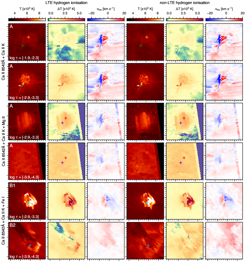
Figure 14: Inversion maps assuming hydrogen ionisation in LTE (left-hand three columns) and in non-LTE (right-hand three columns). Each set of columns has the same format as the left-hand three columns of e.g. Fig. 4, i.e. showing from left to right the temperature, the temperature difference to the input FAL-C temperature and the line-of-sight velocity. The maps correspond to inversions combining Ca ii 8542 Å and Ca ii  K for event A (top two rows), Ca ii and Mg ii for the same event (middle two rows), and Ca ii and Fe i for event B (bottom two rows). Coloured markers correspond to pixels for which detailed profiles are shown in Fig. 15 and are overlaid in the first and third columns (except for the middle two rows where they have been overlaid in the second and fourth column panels instead for better visibility). These sampling locations are the same as the identically coloured locations in Figs. 4 (top two rows), 10 (middle two rows) and 6 (bottom two rows). Major tick marks are spaced 1^′′ apart for all panels.

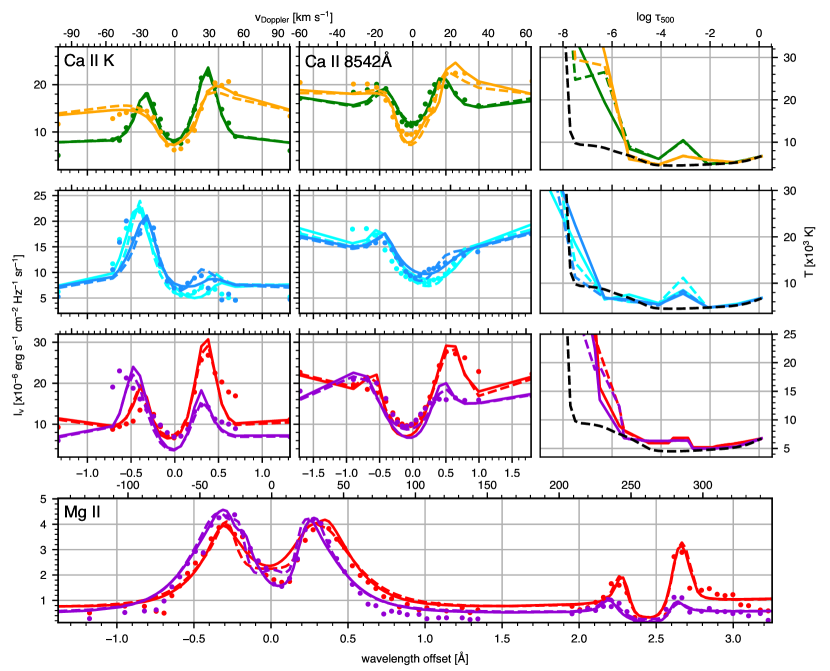
Figure 15: Spectral line and temperature profiles for six selected pixels in Events A (top and bottom two rows) and B (second row) at the identically coloured locations marked in Fig. 14. The left-hand, middle and bottom panels show fits assuming hydrogen ionisation in LTE (dashed lines) and non-LTE (solid lines) to the observed profiles (filled circles) for Ca ii  K (left panel in the first three rows), Ca ii 8542 Å (middle panel in the same rows) and Mg ii (bottom panel). The corresponding temperature stratification (right-hand panels) is shown using the same colour coding, along with the FAL-C input temperature for reference (dashed black line).

The temperature stratifications exhibit more significant changes, though mostly above $\hbox{log $\tau_{500}$}\!=\!-$5 to $-$6 (where the sensitivity of the spectral lines is minimal). The localised temperature increase around $\hbox{log $\tau_{500}$}\!=\!-$3 is practically unchanged in magnitude for all except the cyan sampling. When assuming non-LTE electron densities, the chromospheric temperature plateaus around 2.5–3.0 $\times 10^{4}$ K for the Ca ii inversions in the top row disappear and for Event B (second row) the transition region temperature rise is moved to slightly lower heights, while for the inversions with Mg ii the opposite is the case in exchange for a steeper temperature increase. However, given the highly reduced sensitivity of both Ca ii and Mg ii lines above $\hbox{log $\tau_{500}$}\!=\!-$6 (as also evidenced by the response functions to temperature discussed further down) the presence or absence of the temperature plateaus at those heights is not well-constrained by the spectral profiles and should thus be interpreted with great care.

Notwithstanding, these changes are not surprising considering the differences in the electron density stratification depending on the LTE or non-LTE ionisation assumption. Figure 16 presents these densities as function of log $\tau_{500}$ for all samplings shown in Fig. 15. As one would expect for the lower atmosphere, the differences below $\hbox{log $\tau_{500}$}\!=\!-$2 to $-$2.5 are negligible for all samplings and where those from Event A (green, orange and red) exhibit only minor offsets between the LTE and non-LTE electron densities around the temperature peak at $\hbox{log $\tau_{500}$}\!=\!-$3, the deviations are more promininent for Event B (blue and cyan in the middle panel). This is consistent with the similarity in the temperature enhancement in the case of LTE versus non-LTE (Fig. 15, last column) around $\hbox{log $\tau_{500}$}\!=\!-$3 for the Event A samplings, while those for Event B are visibly different (by over 2600 K for the cyan sampling). Above $\hbox{log $\tau_{500}$}\!=\!-$4 to $-$5 the LTE and non-LTE densities are disparate for all pixels, in most cases also showing the largest deviations, which again coincides with a marked change in temperature stratification above those heights.

Finally, Fig. 17 presents the wavelength-dependent response functions to temperature perturbations for three of the previously considered samplings (red, green and cyan), with positive response in red and negative response in black. These show that in the line wings where the events are best viewed (i.e. the peaks at $\pm$30 km s^-1 for Ca ii  K, $\pm$20 km s^-1 for Ca ii 8542 Å, and out at $\pm$(40–50) km s^-1 for Mg ii  k) the peak response (blue lines) covers a range from $\hbox{log $\tau_{500}$}\!=\!-$2.5 to $-$4 for Ca ii and up to $-$5 for Mg ii, irrespective of the electron density choice and coinciding with the lower-atmospheric temperature enhancements as shown in Fig. 15. In addition, at the red wing enhancement of the red sampling (left hand and bottom panels) both the Ca ii, Mg ii  k and the triplet lines exhibit the strongest response to temperature at similar log $\tau_{500}$ heights. The choice of LTE versus non-LTE electron densities primarily affects the line cores, being sensitive to temperature perturbations at $\hbox{log $\tau_{500}$}\!=\!0.5-1.0$ higher heights (e.g. the red Ca ii  K and Mg ii  k or the cyan Ca ii samplings) in the LTE case, while there is little to no effect in the line wings. This may also explain why the largest differences are observed in the Mg ii  k line core, as its response to temperature perturbations reaches to higher heights than Ca ii.

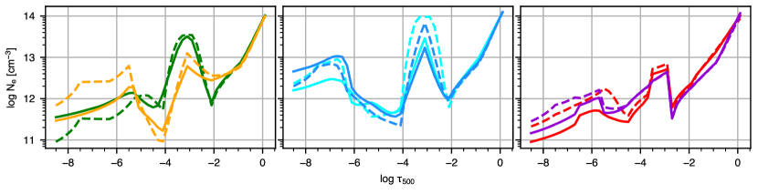
Figure 16: Logarithm of electron density $N_{\rm e}$ as function of log $\tau_{500}$ in the selected pixels from Figs. 14 and 15, with identical colour coding. The curves display the densities consistent with either LTE (dashed) or non-LTE (solid) hydrogen ionisation.

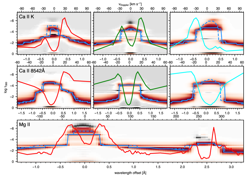
Figure 17: Response functions to temperature with log $\tau_{500}$ as function of wavelength in Ca ii  K (top row), Ca ii 8542 Å (middle row) and Mg ii (bottom panel) for three of the selected pixels from Figs. 14 and 15. Results are shown for the red sampling (first column and bottom panel) and green sampling (second column) of event A, and the cyan sampling of event B (third column), under the assumption of non-LTE hydrogen ionisation. Corresponding observed Ca ii and Mg ii profiles are shown for reference and have been plotted on arbitrary scale to maximise visiblity of profile features. In each panel the response function is displayed in red-white-black colour scale (with red being positive response, black negative and white none), at each wavelength normalised to its maximum with height log $\tau_{500}$. The blue lines indicate the log $\tau_{500}$ heights as function of wavelength for which the response function peaks in the case of LTE (dashed) and non-LTE (solid) electron densities.

Considering these results, our bottom line conclusion is therefore that when inverting Ca ii and Mg ii for Ellerman bombs with UV burst signature the assumption of LTE hydrogen ionisation is adequate as it leads to essentially the same results as when assuming non-LTE hydrogen ionisation. As Si iv is also sensitive to temperature perturbations at higher heights, electron densities consistent with non-LTE ionisation may be required for a correct description of the problem in that case.