Virtual Element for the Buckling Problem of Kirchhoff-Love plates
Dedicated to Rodolfo Rodríguez on his 65th birthday

Abstract

In this paper, we develop a virtual element method (VEM) of high order to solve the fourth order plate buckling eigenvalue problem on polygonal meshes. We write a variational formulation based on the Kirchhoff-Love model depending on the transverse displacement of the plate. We propose a $C^{1}$ conforming virtual element discretization of arbitrary order $k\geq 2$ and we use the so-called Babuška–Osborn abstract spectral approximation theory to show that the resulting scheme provides a correct approximation of the spectrum and prove optimal order error estimates for the buckling modes (eigenfunctions) and a double order for the buckling coefficients (eigenvalues). Finally, we report some numerical experiments illustrating the behaviour of the proposed scheme and confirming our theoretical results on different families of meshes.

1 Introduction

In this paper we analyze a conforming $C^{1}$ virtual element approximation of an eigenvalue problem arising in Structural Mechanics: the elastic stability of plates, in particular the so-called buckling problem. This problem has attracted much interest since it is frequently encountered in several engineering applications such as car or aircraft design. In particular, we will focus on thin plates which are modeled by the Kirchhoff–Love equations.

The buckling problem for plates can be formulated as a spectral problem of fourth order whose solution is related with the limit of elastic stability of the plate (i.e., eigenvalues-buckling coefficients and eigenfunctions-buckling modes). This problem has been studied with several finite element methods, for instance, conforming and non-conforming discretizations, mixed formulations. We cite as a minimal sample of them [17, 20, 26, 31, 32, 34, 38, 41].

The aim of the present paper is to introduce and analyze a virtual element method (VEM) to solve the buckling problem. The VEM has been introduced in [6] and has been applied successfully in a large range of problems in fluid and solid mechanics; see for instance [2, 3, 4, 7, 8, 9, 11, 12, 15, 16, 21, 22, 23, 24, 33, 40, 43, 44]. Regarding VEM for spectral problems, we mention the following recent works [14, 27, 28, 35, 36, 37, 39].

One important advantage of VEM is the possibility of easily implement highly regular discrete spaces to solve fourth order partial differential equations [3, 19, 24]. It is very well known that the construction of conforming finite elements to $H^{2}$ is difficult in general, since they generally involve a large number of degrees of freedom (see [25]). Here, we follow the VEM approach presented in [19, 24] to build global discrete spaces of $C^{1}$ of arbitrary order that are simple in terms of degrees of freedom and coding aspects to solve an eigenvalue problem modelling the plate buckling problem.

More precisely, we will propose a $C^{1}$ Virtual Element Method of arbitrary order $k\geq 2$ to approximate the buckling coefficients and modes of the plate buckling problem on general polygonal meshes. Based on the transverse displacements of the midplane of a thin plate subjected to a symmetric stress tensor field, we propose and analyze a variational formulation in $H^{2}$. We characterize the continuous spectrum of the problem through a certain continuous, compact and self-adjoint operator. Then, we exploit the ability of VEM in order to construct highly regular discrete spaces and propose a conforming discretization of the buckling eigenvalue problem in $H^{2}$ which is an extension of the discrete virtual space introduced in [3, 19]. We construct projection operators in order to write bilinear forms that are fully computable. In particular, to discretize the right hand side of the eigenvalue problem we propose a simple bilinear form which does not need any stabilization. This make possible to use directly the so-called Babuška–Osborn abstract spectral approximation theory (see [5]) to show that under standard shape regularity assumptions the resulting virtual element scheme provides a correct approximation of the spectrum and prove optimal order error estimates for the eigenfunctions and a double order for the eigenvalues. The proposed VEM method provides an attractive and competitive alternative to solve the fourth order plate buckling eigenvalue problem in term of its computational cost. For instance, in the lowest order configuration $(k=2)$, the computational cost is almost $3N_{v}$, where $N_{v}$ denotes the number of vertices in the polygonal mesh. For $k=3$, the computational cost is almost $3N_{v}+N_{e}$, where $N_{e}$ denotes the number of edges in the polygonal mesh.

This paper is structured as follows: In Section 2, we present the variational formulation for the plate buckling eigenvalue problem. We define a solution operator whose spectrum allows us to characterize the spectrum of the buckling problem. In Section 3 we introduce the virtual element discretization of arbitrary degree $k\geq 2$, describe the spectrum of a discrete solution operator and prove some auxiliary results. In Section 4, we prove that the numerical scheme presented in this work provides a correct spectral approximation and establish optimal order error estimates for the eigenvalues and eigenfunctions. Finally, in Section 5 we report some numerical tests that confirm the theoretical analysis developed.

Throughout the article we will use standard notations for Sobolev spaces, norms and seminorms. Moreover, we will denote by $C$ a generic constant independent of the mesh parameter $h$, which may take different values in different occurrences.

2 Presentation of the continuous spectral problem.

Let $\Omega\subseteq\mathbb{R}^{2}$ be a polygonal bounded domain corresponding to the mean surface of a plate in its reference configuration. The plate is assumed to be homogeneous, isotropic, linearly elastic, and sufficiently thin as to be modeled by Kirchhoff-Love equations. The buckling eigenvalue problem of a clamped plate, which is subjected to a plane stress tensor field $\boldsymbol{\eta}:\Omega\to\mathbb{R}^{2\times 2}$ with $\boldsymbol{\eta}\neq 0$ reads as follows:

$$\left\{\begin{array}[]{lll}\Delta^{2}u=-\lambda\mathop{\mathrm{\,div}}\nolimits(\boldsymbol{\eta}\nabla u)&\mbox{in }\Omega,\\ u=\partial_{\nu}u=0&\mbox{on }\Gamma.\end{array}\right.$$ (2.1)

The unknowns of this eigenvalue problem are the deflection of the plate $u$ (buckling modes) and the eigenvalue $\lambda$ (scaled buckling coefficients). We have denoted by $\partial_{\nu}$ the normal derivative. To simplify the notation we have taken the Young modulus and the density of the plate, both equal to 1. In addition, the stress tensor field is assumed to satisfy the following equilibrium equations:

$$\boldsymbol{\eta}^{\rm t}=\boldsymbol{\eta} \quad\mbox{in }\Omega,$$

$$\mathop{\bf{div}}\nolimits\boldsymbol{\eta}=0 \quad\mbox{in }\Omega.$$

In the remain of this section and in Section 3, it is enough to consider $\boldsymbol{\eta}\in L^{\infty}(\Omega)^{2\times 2}$. However, we will assume some additional regularity which will be used in the proof of Theorem 4.4. In addition, we do not need to assume $\boldsymbol{\eta}$ to be positive definite. Let us remark that, in practice, $\boldsymbol{\eta}$ is the stress distribution on the plate subjected to in-plane loads, which does not need to be positive definite [42].

2.1 The continuous formulation.

In this section we will present and analyze a variational formulation associated with the spectral problem. We will also introduce the so-called solution operator whose spectra will be related to the solutions of the continuous spectral problem (2.1).

In order to write the variational formulation of the spectral problem, we introduce the following symmetric bilinear forms in $H_{0}^{2}(\Omega)$:

$$a(u,v):=\int_{\Omega}D^{2}u:\,D^{2}v,\qquad b(u,v):=\int_{\Omega}(\boldsymbol{\eta}\nabla u)\cdot\nabla v,$$

where $":"$ denotes the usual scalar product of $2\times 2$-matrices, $D^{2}v:=(\partial_{ij}v)_{1\leq i,j\leq 2}$ denotes the Hessian matrix of $v$. It is easy to see that $a(\cdot,\cdot)$ is an inner-product in $H_{0}^{2}(\Omega)$.

The variational formulation of the eigenvalue problem (2.1) is given as follows:

Problem 1.

Find $(\lambda,u)\in\mathbb{R}\times{H_{0}^{2}(\Omega)}$, $u\neq 0$, such that

$$\begin{array}[]{llll}a(u,v)=\lambda b(u,v)\qquad\forall v\in{H_{0}^{2}(\Omega)}.\end{array}$$ (2.2)

The following result establishes that the bilinear form $a(\cdot,\cdot)$ is elliptic in $H_{0}^{2}(\Omega)$.

Lemma 2.1.

There exists a constant $\alpha_{0}>0$, depending on $\Omega$, such that

$$a(v,v)\geq\alpha_{0}\left\|v\right\|_{2,\Omega}^{2}\qquad\forall v\in{H_{0}^{2}(\Omega)}.$$

Proof.

The result follows immediately from the fact that $\|D^{2}v\|_{0,\Omega}$ is a norm on ${H_{0}^{2}(\Omega)}$, equivalent with the usual norm. ∎

Remark 2.1.

We have that $\lambda\neq 0$ in problem (2.2). Moreover, it is easy to prove, using the symmetry of $\boldsymbol{\eta}$, that all the eigenvalues are real (not necessarily positive). We also have that $b(u,u)\neq 0$.

Next, in order to analyze the variational eigenvalue problem (2.2), we introduce the following solution operator:

$$T:\ {H_{0}^{2}(\Omega)} \longrightarrow{H_{0}^{2}(\Omega)},$$

$$f \longmapsto Tf:=w,$$

where $w\in{H_{0}^{2}(\Omega)}$ is the unique solution (as a consequence of Lemma 2.1) of the following source problem:

$$a(w,v)=b(f,v)\qquad\forall v\in{H_{0}^{2}(\Omega)}.$$ (2.3)

We have that the linear operator $T$ is well defined and bounded. Notice that $(\lambda,u)\in\mathbb{R}\times{H_{0}^{2}(\Omega)}$ solves problem (2.2) if and only if $Tu=\mu u$ with $\mu\neq 0$ and $u\neq 0$, in which case $\mu:=\frac{1}{\lambda}$. In addition, using the symmetry of $\boldsymbol{\eta}$, we can deduce that $T$ is self-adjoint with respect to the inner product $a(\cdot,\cdot)$ in ${H_{0}^{2}(\Omega)}$. Indeed, given $f,g\in{H_{0}^{2}(\Omega)}$,

$$a(Tf,g)=b(f,g)=b(g,f)=a(Tg,f)=a(f,Tg).$$

On the other hand, the following is an additional regularity result for the solution of problem (2.3) and consequently, for the eigenfunctions of $T$.

Lemma 2.2.

There exists $s_{\Omega}>1/2$ such that the following results hold:

• For all $f\in H^{1}(\Omega)$, there exists a positive constant $C>0$ such that any solution $w$ of the source problem (2.3) satisfies $w\in H^{2+\tilde{s}}(\Omega)$ with $\tilde{s}:=\min\{s_{\Omega},1\}$ and

  $$\|w\|_{2+\tilde{s},\Omega}\leq C\|f\|_{1,\Omega}.$$

• If $(\lambda,u)$ is an eigenpair of the spectral problem (2.2), there exist $s>1/2$ and a positive constant $C$ depending only on $\Omega$ such that $u\in H^{2+s}(\Omega)$ and

  $$\|u\|_{2+s,\Omega}\leq C\|u\|_{2,\Omega}.$$

Proof.

The proof follows from the classical regularity result for the biharmonic problem with its right-hand side in $L^{2}(\Omega)$ (cf. [30]). ∎

Therefore, because of the compact inclusion ${H^{2+s}(\Omega)}\hookrightarrow{H_{0}^{2}(\Omega)}$, $T$ is a compact operator. Thus, we finish this section with the following spectral characterization result.

Lemma 2.3.

The spectrum of $T$ satisfies $\mathop{\mathrm{sp}}\nolimits(T)=\{0\}\cup\left\{\mu_{k}\right\}_{k\in\mathbb{N}}$, where $\left\{\mu_{k}\right\}_{k\in\mathbb{N}}$ is a sequence of real eigenvalues which converges to $0$. The multiplicity of each eigenvalue is finite.

3 Spectral approximation.

In this section, we will write a VEM discretization of the spectral problem (2.2). With this aim, we start with the mesh construction and the assumptions considered to introduce the discrete virtual element spaces.

Let $\left\{\mathcal{T}_{h}\right\}_{h}$ be a sequence of decompositions of $\Omega$ into polygons $K$ we will denote by $h_{K}$ the diameter of the element $K$ and $h$ the maximum of the diameters of all the elements of the mesh, i.e., $h:=\max_{K\in\mathcal{T}_{h}}h_{K}$. In what follows, we denote by $N_{K}$ the number of vertices of $K$, by $e$ a generic edge of $\left\{\mathcal{T}_{h}\right\}_{h}$ and for all $e\in\partial K$, we define a unit normal vector $\nu_{K}^{e}$ that points outside of $K$.

In addition, we will make the following assumptions as in [6, 14]: there exists a positive real number $C_{\mathcal{T}}$ such that, for every $h$ and every $K\in\mathcal{T}_{h}$,

• $K\in\mathcal{T}_{h}$ is star-shaped with respect to every point of a ball of radius $C_{\mathcal{T}}h_{K}$;

• the ratio between the shortest edge and the diameter $h_{K}$ of $K$ is larger than $C_{\mathcal{T}}$.

In order to introduce the discretization, for every integer $k\geq 2$ and for every polygon $K$, we define the following finite dimensional space:

$$\widetilde{V}_{h}^{K}:=\left\{v_{h}\in{H^{2}(K)}:\Delta^{2}v_{h}\in\mathbb{P}_{k-2}(K),v_{h}|_{\partial K}\in C^{0}(\partial K),v_{h}|_{e}\in\mathbb{P}_{r}(e)\,\,\forall e\in\partial K,\right.$$

$$\left.\nabla v_{h}|_{\partial K}\in C^{0}(\partial K)^{2},\partial_{\nu_{K}^{e}}v_{h}|_{e}\in\mathbb{P}_{s}(e)\,\,\forall e\in\partial K\right\},$$

where $r:=\max\{3,k\}$ and $s:=k-1$.

This space has been recently considered in [24] to obtain optimal error estimates for fourth order PDEs and it can be seen as an extension of the $C^{1}$ virtual space introduced in [19] to solve the bending problem of thin plates. Here, we will consider the same space together with an enhancement technique (cf. [1]) to build a computable right hand of the buckling eigenvalue problem.

It is easy to see that any $v_{h}\in\widetilde{V}_{h}^{K}$ satisfies the following conditions:

• the trace (and the trace of the gradient) on the boundary of $K$ is continuous;

• $\mathbb{P}_{k}(K)\subseteq\widetilde{V}_{h}^{K}$.

In $\widetilde{V}_{h}^{K}$ we define the following five sets of linear operators. For all $v_{h}\in\widetilde{V}_{h}^{K}$:

• evaluation of $v_{h}$ at the $N_{K}$ vertices of $K$;

• evaluation of $\nabla v_{h}$ at the $N_{K}$ vertices of $K$;

• For $r>3$, the moments $\int_{e}q(\xi)v_{h}(\xi)d\xi\qquad\quad\forall q\in\mathbb{P}_{r-4}(e),\quad\forall\mbox{ edge }e;$

• For $s>1$, the moments $\int_{e}q(\xi)\partial_{\nu_{K}^{e}}v_{h}(\xi)d\xi\quad\ \forall q\in\mathbb{P}_{s-2}(e),\quad\forall\mbox{ edge }e;$

• For $k\geq 4$, the moments $\int_{K}q(\boldsymbol{x})v_{h}(\boldsymbol{x})d\boldsymbol{x}\qquad\forall q\in\mathbb{P}_{k-4}(K),\ \ \forall\mbox{ polygon }K$.

In order to construct the discrete scheme, we need some preliminary definitions. First, we note that bilinear form $a(\cdot,\cdot)$, introduced in the previous section, can be split as follows:

$$a(u,v)=\sum_{K\in\mathcal{T}_{h}}a_{K}(u,v),\qquad u,v\in{H_{0}^{2}(\Omega)},$$

with

$$a_{K}(u,v):=\int_{K}D^{2}u:\,D^{2}v,\qquad u,v\in{H^{2}(K)}.$$

Now, we define the projector $\Pi_{K}^{k,D}:H^{2}(K)\to\mathbb{P}_{k}(K)\subseteq\widetilde{V}_{h}^{K}$ as the solution of the following local problems (in each element $K$):

$$a_{K}\big{(}\Pi_{K}^{k,D}v,q\big{)}=a_{K}(v,q)\qquad\forall q\in\mathbb{P}_{k}(K)\quad\forall v\in H^{2}(K),$$ (3.1a)

$$\widehat{\Pi_{K}^{k,D}v}=\widehat{v},\quad\widehat{\nabla\Pi_{K}^{k,D}v}=\widehat{\nabla v},$$ (3.1b)

where $\widehat{v}$ is defined as follows:

$$\widehat{v}:=\frac{1}{N_{K}}\sum_{i=1}^{N_{K}}v(\mathop{\mathrm{\,v}}\nolimits_{i})\qquad\forall v\in C^{0}(\partial K)$$

and $\mathop{\mathrm{\,v}}\nolimits_{i},1\leq i\leq N_{K}$, are the vertices of $K$.

We observe that bilinear form $a_{K}(\cdot,\cdot)$ has a non-trivial kernel given by $\mathbb{P}_{1}(K)$. Hence, the role of condition (3.1b) is to select an element of the kernel of the operator.

It is easy to see that operator $\Pi_{K}^{k,D}$ is well defined on $\widetilde{V}_{h}^{K}$. Moreover, the following result states that for all $v\in\widetilde{V}_{h}^{K}$ the polynomial $\Pi_{K}^{k,D}v$ can be computed using the output values of the sets ${\bf D_{1}}-{\bf D_{5}}$.

Lemma 3.1.

The operator $\Pi_{K}^{k,D}:\widetilde{V}_{h}^{K}\to\mathbb{P}_{k}(K)$ is explicitly computable for every $v\in\widetilde{V}_{h}^{K}$, using only the information of the linear operators in ${\bf D_{1}}-{\bf D_{5}}$.

Proof.

For all $v_{h}\in\widetilde{V}_{h}^{K}$ we integrate twice by parts on the right-hand side of (3.1a). We obtain

$$a(v_{h},q) =\int_{K}D^{2}v_{h}:D^{2}q$$

$$=\int_{K}\Delta^{2}qv_{h}-\int_{\partial K}\mathop{\bf{div}}\nolimits(D^{2}q)\cdot\nu_{K}v_{h}+\int_{\partial K}D^{2}q\nu_{K}\cdot\nabla v_{h}.$$ (3.2)

It is easy to see that since $\Delta^{2}q\in\mathbb{P}_{k-4}(K)$ hence the first integral in the right-hand side of (3.2) is computable using the output values of the set ${\bf D_{5}}$. We also note that the boundary integrals of (3.2) only depends on the boundary values of $v_{h}$ and $\nabla v_{h}$, so they are computable using the output values of the sets ${\bf D_{1}}-{\bf D_{4}}$. On the other hand, the kernel part of $\Pi_{K}^{k,D}$ (cf. (3.1b)) is computable using the output values of the sets ${\bf D_{1}}-{\bf D_{2}}$. ∎

We introduce our local virtual space:

$$V^{K}_{h}:=\left\{v_{h}\in\widetilde{V}_{h}^{K}:\int_{K}(\Pi_{K}^{k,D}v_{h})q=\int_{K}v_{h}q\qquad\forall q\in\mathbb{P}_{k-3}^{*}(K)\cup\mathbb{P}_{k-2}^{*}(K)\right\}.$$

where $\mathbb{P}_{\ell}^{*}(K)$ denotes homogeneous polynomials of degree $\ell$ with the convention that $\mathbb{P}_{-1}^{*}(K)=\{0\}$.

Note that $V_{h}^{K}\subseteq\widetilde{V}_{h}^{K}$. Thus, the linear operator $\Pi_{K}^{k,D}$ is well defined on $V_{h}^{K}$ and computable only using the output values of the sets ${\bf D_{1}}-{\bf D_{5}}$. We also have that $\mathbb{P}_{k}(K)\subseteq V^{K}_{h}$. This will guarantee the good approximation properties of the space.

Moreover, it has been established in [24] that the set of linear operators ${\bf D_{1}}-{\bf D_{5}}$ constitutes a set of degrees of freedom for $V_{h}^{K}$.

Now, we consider the $L^{2}(K)$ orthogonal projector onto $\mathbb{P}_{k-2}(K)$ as follows: we define $\Pi_{K}^{k-2}:L^{2}(K)\to\mathbb{P}_{k-2}(K)$ for each $v\in L^{2}(K)$ by

$$\int_{K}(\Pi_{K}^{k-2}v)q=\int_{K}vq\qquad\forall q\in\mathbb{P}_{k-2}(K).$$ (3.3)

Next, due to the particular property appearing in definition of the space $V^{K}_{h}$, it can be seen that the right hand side in (3.3) is computable using $\Pi_{K}^{k,D}v$, and the degrees of freedom given by ${\bf D_{5}}$ and thus $\Pi_{K}^{k-2}v$ depends only on the values of the degrees of freedom given by ${\bf D_{1}}-{\bf D_{5}}$ when $v\in V^{K}_{h}$.

In order to discretize the right hand side of the buckling eigenvalue problem, we will consider the following projector onto $\mathbb{P}_{k-1}(K)^{2}$: we define $\boldsymbol{\Pi}_{K}^{k-1}:H^{1}(K)\to\mathbb{P}_{k-1}(K)^{2}$ for each $v\in H^{1}(K)$ by

$$\int_{K}(\boldsymbol{\Pi}_{K}^{k-1}\nabla v)\cdot{\bf q}=\int_{K}\nabla v\cdot{\bf q}\quad\forall{\bf q}\in\mathbb{P}_{k-1}(K)^{2}.$$

In addition, we observe that the for any $v_{h}\in V^{K}_{h}$, the vector function $\boldsymbol{\Pi}_{K}^{k-1}\nabla v_{h}$ can be explicitly computed from the degrees of freedom ${\bf D_{1}}-{\bf D_{5}}$. In fact, in order to compute $\boldsymbol{\Pi}_{K}^{k-1}\nabla v_{h}$, for all $K\in\mathcal{T}_{h}$ we must be able to calculate the following:

$$\int_{K}\nabla v_{h}\cdot{\bf q}\qquad\forall{\bf q}\in\mathbb{P}_{k-1}(K)^{2}.$$

From an integration by parts, we have

$$\begin{split}\int_{K}\nabla v_{h}\cdot{\bf q}&=-\int_{K}v_{h}\mathop{\mathrm{\,div}}\nolimits{\bf q}+\int_{\partial K}v_{h}({\bf q}\cdot\nu_{K})\qquad\forall{\bf q}\in\mathbb{P}_{k-1}(K)^{2},\\ &=-\int_{K}\Pi_{K}^{k-2}v_{h}\mathop{\mathrm{\,div}}\nolimits{\bf q}+\int_{\partial K}v_{h}({\bf q}\cdot\nu_{K})\qquad\forall{\bf q}\in\mathbb{P}_{k-1}(K)^{2}.\end{split}$$

The first term on the right-hand side above depends only on the $\Pi_{K}^{k-2}v_{h}$ and this depends on the values of the degrees of freedom ${\bf D_{1}}-{\bf D_{5}}$ (cf. (3.3)). The second term can also be computed since ${\bf q}$ is a polynomial of degree $k-1$ on each edge and therefore is uniquely determined by the values of ${\bf D_{1}}-{\bf D_{5}}$.

Now, we are ready to define our global virtual space to solve the plate buckling eigenvalue problem, this is defined as follows:

$$V_{h}:=\Big{\{}v_{h}\in H_{0}^{2}(\Omega):v_{h}|_{K}\in V_{h}^{K}\Big{\}}.$$ (3.4)

In what follows, we discuss the construction of the discrete version of the local forms. With this aim, we consider $s_{K}^{D}(\cdot,\cdot)$ any symmetric positive definite and computable bilinear form to be chosen as to satisfy:

$$c_{0}a_{K}(v_{h},v_{h})\leq s_{K}^{D}(v_{h},v_{h})\leq c_{1}a_{K}(v_{h},v_{h})\quad\forall v_{h}\in V_{h}^{K}\quad\mbox{with }\quad\Pi_{K}^{k,D}v_{h}=0.$$ (3.5)

Then, we set

$$a_{h}(u_{h},v_{h}):=\sum_{K\in\mathcal{T}_{h}}a_{h,K}(u_{h},v_{h}),\qquad u_{h},v_{h}\in V_{h},$$

$$b_{h}(u_{h},v_{h}):=\sum_{K\in\mathcal{T}_{h}}b_{h,K}(u_{h},v_{h}),\qquad u_{h},v_{h}\in V_{h},$$

with $a_{h,K}(\cdot,\cdot)$ and $b_{h,K}(\cdot,\cdot)$ are the local bilinear forms on $V^{K}_{h}\times V^{K}_{h}$ defined by

$$a_{h,K}(u_{h},v_{h}):=a_{K}\big{(}\Pi_{K}^{k,D}u_{h},\Pi_{K}^{k,D}v_{h}\big{)}+s_{K}^{D}\big{(}u_{h}-\Pi_{K}^{k,D}u_{h},v_{h}-\Pi_{K}^{k,D}v_{h}\big{)},$$ (3.6)

$$b_{h,K}(u_{h},v_{h}):=\int_{K}\boldsymbol{\eta}\boldsymbol{\Pi}_{K}^{k-1}\nabla u_{h}\cdot\boldsymbol{\Pi}_{K}^{k-1}\nabla v_{h}.$$ (3.7)

Notice that the bilinear form $s_{K}^{D}(\cdot,\cdot)$ has to be actually computable for $u_{h},v_{h}\in V^{K}_{h}$.

Proposition 3.1.

The local bilinear form $a_{h,K}(\cdot,\cdot)$ on each element $K$ satisfy

• Consistency: for all $h>0$ and for all $K\in\mathcal{T}_{h}$, we have that

  $$a_{h,K}(p,v_{h})=a_{K}(p,v_{h})\qquad\forall p\in\mathbb{P}_{k}(K),\quad\forall v_{h}\in V^{K}_{h},$$ (3.8)

• Stability and boundedness: There exist two positive constants $\alpha_{1},\alpha_{2}$, independent of $K$, such that:

  $$\alpha_{1}a_{K}(v_{h},v_{h}) \leq a_{h,K}(v_{h},v_{h})\leq\alpha_{2}a_{K}(v_{h},v_{h}) \qquad\forall v_{h}\in V^{K}_{h}.$$ (3.9)

3.1 The discrete eigenvalue problem.

Now, we are in a position to write the virtual element discretization of Problem 1 as follows.

Problem 2.

Find $(\lambda_{h},u_{h})\in\mathbb{R}\times V_{h}$, $u_{h}\neq 0$, such that

$$a_{h}(u_{h},v_{h})=\lambda_{h}b_{h}(u_{h},v_{h})\qquad\forall v_{h}\in V_{h}.$$ (3.10)

We observe that by virtue of (3.9), the bilinear form $a_{h}(\cdot,\cdot)$ is bounded. Moreover, as shown in the following lemma, it is also uniformly elliptic.

Lemma 3.2.

There exists a constant $\alpha>0$, independent of $h$, such that

$$a_{h}(v_{h},v_{h})\geq\alpha\left\|v_{h}\right\|_{2,\Omega}^{2}\qquad\forall v_{h}\in V_{h}.$$

Proof.

Thanks to (3.9) and Lemma 2.1, it is easy to check that the above inequality holds with $\alpha:=\alpha_{0}\min\left\{\alpha_{1},1\right\}$. ∎

In order to analyze the discrete problem, we introduce the solution operator associated to Problem 2 as follows:

$$T_{h}:H_{0}^{2}(\Omega) \longrightarrow H_{0}^{2}(\Omega),$$

$$f \longmapsto T_{h}f:=w_{h},$$

with $w_{h}$ the unique solution of the following source problem

$$a_{h}(w_{h},v_{h})=b_{h}(f,v_{h})\qquad\forall v_{h}\in V_{h}.$$ (3.11)

Note that the ellipticity of $a_{h}(\cdot,\cdot)$ established in Lemma 3.2, the boundedness of the right hand side (cf. (3.7)) and Lax-Milgram Lemma guarantee that $T_{h}$ is well defined. Moreover, as in the continuous case, $(\lambda_{h},u_{h})\in\mathbb{R}\times V_{h}$ solves problem (3.10) if and only if $T_{h}u_{h}=\mu_{h}u_{h}$ with $\mu_{h}\neq 0$ and $u_{h}\neq 0$, in which case $\mu_{h}:=\frac{1}{\lambda_{h}}$.

Remark 3.1.

The same arguments leading to Remark 2.1 allow us to show that any solution of (3.10) satisfies $\lambda_{h}\neq 0$. Moreover, $b_{h}(u_{h},u_{h})\neq 0$ also holds true.

Moreover from the definition of $a_{h}(\cdot,\cdot)$ and $b_{h}(\cdot,\cdot)$ we can check that $T_{h}$ is self-adjoint with respect to inner product $a_{h}(\cdot,\cdot)$. Therefore, we can describe the spectrum of the solution operator $T_{h}$.

Now, we are in position to write the following characterization of the spectrum of the solution operator.

Theorem 3.1.

The spectrum of $T_{h}$ consists of $M_{h}:=\mathop{\mathrm{\,dim}}\nolimits(V_{h})$ eigenvalues, repeated according to their respective multiplicities. The spectrum decomposes as follows: $\mathop{\mathrm{sp}}\nolimits(T_{h})=\{0\}\cup\{\mu_{h}\}_{k=1}^{\kappa}$, where $\kappa=M_{h}-\mathop{\mathrm{\,dim}}\nolimits Z_{h}$ with $Z_{h}:=\left\{u_{h}\in V_{h}:\,b_{h}(u_{h},v_{h})=0\quad\forall v_{h}\in V_{h}\right\}$. The eigenvalues $\mu_{h}$ are all real and non-zero.

4 Convergence and error estimates.

In this section we will establish convergence and error estimates of the proposed VEM discretization. With this aim, we will prove that $T_{h}$ provides a correct spectral approximation of $T$ using the classical theory for compact operators (see [5]).

We start with the following approximation result, on star-shaped polygons, which is derived by interpolation between Sobolev spaces (see for instance [29, Theorem I.1.4] from the analogous result for integer values of $s$). We mention that this result has been stated in [6, Proposition 4.2] for integer values and follows from the classical Scott-Dupont theory (see [18] and [3, Proposition 3.1]):

Proposition 4.1.

There exists a constant $C>0$, such that for every $v\in H^{\delta}(K)$ there exists $v_{\pi}\in\mathbb{P}_{k}(K)$, $k\geq 0$ such that

$$|v-v_{\pi}|_{\ell,K}\leq Ch_{K}^{\delta-\ell}|v|_{\delta,K}\quad 0\leq\delta\leq k+1,\ell=0,\ldots,[\delta],$$

with $[\delta]$ denoting largest integer equal or smaller than $\delta\in{\mathbb{R}}$.

In what follows, we write several auxiliary results which will be useful in the forthcoming analysis. First, we write standard error estimations for the projector $\boldsymbol{\Pi}_{K}^{k-1}$.

Lemma 4.1.

There exists $C>0$ independent of $h$ such that for all ${\bf v}\in H^{\delta}(K)^{2}$

$$\|{\bf v}-\boldsymbol{\Pi}_{K}^{k-1}{\bf v}\|_{0,K}\leq Ch_{K}^{\delta}|{\bf v}|_{\delta,K}\quad 0\leq\delta\leq k+1.$$

Now, we present an interpolation result in the virtual space $V_{h}$ (see [3, 13]).

Proposition 4.2.

Assume A1–A2 are satisfied, then for all $v\in H^{s}(K)$ there exist $v_{I}\in V_{h}$ and $C>0$ independent of $h$ such that

$$||v-v_{I}||_{l,K}\leq Ch_{K}^{s-l}|v|_{s,K},\quad l=0,1,2,\quad 2\leq s\leq k+1.$$

Now, in order to prove the convergence of our method, we introduce the following broken $H^{s}$-seminorm ($s=1,2$):

$$|v|_{s,h}:=\Big{(}\sum_{K\in\mathcal{T}_{h}}|v|_{s,K}^{2}\Big{)}^{1/2},$$

which is well defined for every $v\in L^{2}(\Omega)$ such that $v|_{K}\in H^{s}(K)$ for all polygon $K\in\mathcal{T}_{h}$.

Now, with these definitions we have the following results.

Lemma 4.2.

There exists $C>0$ such that, for all $f\in H_{0}^{2}(\Omega)$, if $w=Tf$ and $w_{h}=T_{h}f$, then

$$\left\|\left(T-T_{h}\right)f\right\|_{2,\Omega}=\left\|w-w_{h}\right\|_{2,\Omega}\leq C\Big{(}h||f||_{2,\Omega}+\left\|w-w_{I}\right\|_{2,\Omega}+|w-w_{\pi}|_{2,h}\Big{)},$$

for all $w_{I}\in V_{h}$ and for all $w_{\pi}\in L^{2}(\Omega)$ such that $w_{\pi}|_{K}\in\mathbb{P}_{k}(K)\quad\forall K\in\mathcal{T}_{h}$.

Proof.

Let $f\in H_{0}^{2}(\Omega)$, and $w=Tf$ and $w_{h}=T_{h}f$. For $w_{I}\in V_{h}$, we set $v_{h}:=w_{h}-w_{I}$. Thus

$$||(T-T_{h})f||_{2,\Omega}\leq||w-w_{I}||_{2,\Omega}+||v_{h}||_{2,\Omega}.$$ (4.1)

Now, thanks to Lemma 3.2, the definition of $a_{h,{K}}(\cdot,\cdot)$ and those of $T$ and $T_{h}$, we have

$$\alpha||v_{h}||_{2,\Omega}^{2} \leq a_{h}(v_{h},v_{h})=a_{h}(w_{h},v_{h})-a_{h}(w_{I},v_{h})=a_{h}(w_{h},v_{h})-\sum\limits_{K\in\mathcal{T}_{h}}a_{h,K}(w_{I},v_{h})$$

$$=a_{h}(w_{h},v_{h})-\sum\limits_{K\in\mathcal{T}_{h}}\Big{\{}a_{h,K}(w_{I}-w_{\pi},v_{h})+a_{h,K}(w_{\pi},v_{h})\Big{\}}$$

$$=a_{h}(w_{h},v_{h})-\sum\limits_{K\in\mathcal{T}_{h}}\Big{\{}a_{h,K}(w_{I}-w_{\pi},v_{h})+a_{K}(w_{\pi}-w,v_{h})+a_{K}(w,v_{h})\Big{\}}$$

$$=a_{h}(w_{h},v_{h})-a(w,v_{h})-\sum\limits_{K\in\mathcal{T}_{h}}\Big{\{}a_{h,K}(w_{I}-w_{\pi},v_{h})+a_{K}(w_{\pi}-w,v_{h})\Big{\}}.$$ (4.2)

We bound each term on the right hand side of (4.2). The first term can be estimated as follows

$$a_{h}(w_{h},v_{h})-a(w,v_{h})=b_{h}(f,v_{h})-b(f,v_{h})$$

$$=\sum_{K\in\mathcal{T}_{h}}\Bigg{\{}\int_{K}\big{\{}\boldsymbol{\eta}\boldsymbol{\Pi}_{K}^{k-1}\nabla f\cdot\boldsymbol{\Pi}_{K}^{k-1}\nabla v_{h}-\boldsymbol{\eta}\nabla f\cdot\nabla v_{h}\big{\}}\Bigg{\}}$$

$$=\sum_{K\in\mathcal{T}_{h}}\Bigg{\{}\int_{K}\big{\{}\boldsymbol{\eta}\boldsymbol{\Pi}_{K}^{k-1}\nabla f\cdot\boldsymbol{\Pi}_{K}^{k-1}\nabla v_{h}-\boldsymbol{\eta}\nabla f\cdot\boldsymbol{\Pi}_{K}^{k-1}\nabla v_{h}+\boldsymbol{\eta}\nabla f\cdot\boldsymbol{\Pi}_{K}^{k-1}\nabla v_{h}-\boldsymbol{\eta}\nabla f\cdot\nabla v_{h}\big{\}}\Bigg{\}}$$

$$=\sum_{K\in\mathcal{T}_{h}}\Bigg{\{}\int_{K}\big{\{}\boldsymbol{\eta}\left(\boldsymbol{\Pi}_{K}^{k-1}\nabla f-\nabla f\right)\cdot\boldsymbol{\Pi}_{K}^{k-1}\nabla v_{h}+\boldsymbol{\eta}\nabla f\cdot\left(\boldsymbol{\Pi}_{K}^{k-1}\nabla v_{h}-\nabla v_{h}\right)\big{\}}\Bigg{\}}$$

$$\leq\sum_{K\in\mathcal{T}_{h}}C\Bigg{\{}\|\boldsymbol{\Pi}_{K}^{k-1}\nabla f-\nabla f\|_{0,K}\|\boldsymbol{\Pi}_{K}^{k-1}\nabla v_{h}\|_{0,K}+\|\nabla f\|_{0,K}\|\boldsymbol{\Pi}_{K}^{k-1}\nabla v_{h}-\nabla v_{h}\|_{0,K}\Bigg{\}}$$

$$\leq Ch\|f\|_{2,\Omega}\|v_{h}\|_{2,\Omega},$$

where we have used Lemma 4.1 in the last inequality. Notice taht the constant $C>0$ depends on $\|\boldsymbol{\eta}\|_{\infty}$.

Next, using the stability of $a_{h,K}(\cdot,\cdot)$, the Cauchy-Schwarz and triangular inequalities in the second term on the right hand side of (4.2), we have

$$\alpha\left\|v_{h}\right\|^{2}_{2,\Omega} \leq C\Big{(}h||f||_{2,\Omega}+\left\|w-w_{I}\right\|_{2,\Omega}+|w-w_{\pi}|_{2,h}\Big{)}\|v_{h}\|_{2,\Omega}.$$

Thus, the result follows from the previous bounds together with (4.2). ∎

Now we are in a position to prove that the operator $T_{h}$ converges in norm to $T$.

Theorem 4.1.

For all $f\in H_{0}^{2}(\Omega)$, there exist $\tilde{s}\in(\frac{1}{2},1]$ and $C>0$ independent of $h$ such that

$$||(T-T_{h})f||_{2,\Omega}\leq Ch^{\tilde{s}}||f||_{2,\Omega}.$$

Proof.

The proof is obtained from Lemma 4.2 and Propositions 4.1 and 4.2 and Lemma 2.2. ∎

Next, we will use the classical theory for compact operators (see [5] for instance) in order to prove convergence and error estimates for eigenfunctions and eigenvalues. Indeed, an immediate consequence of Theorem 4.1 is that isolated parts of $\mathop{\mathrm{sp}}\nolimits(T)$ are approximated by isolated parts of $\mathop{\mathrm{sp}}\nolimits(T_{h})$. It means that if $\mu$ is a nonzero eigenvalue of $T$ with algebraic multiplicity $m$, hence there exist $m$ eigenvalues $\mu_{h}^{(1)},\ldots,\mu_{h}^{(m)}$ of $T_{h}$ (repeated according to their respective multiplicities) that will converge to $\mu$ as $h$ goes to zero.

Now, let us denote by $\mathcal{E}$ and $\mathcal{E}_{h}$ the eigenspace associated to the eigenvalue $\mu$ and the spanned of the eigenspaces associated to $\mu_{h}^{(1)},...,\mu_{h}^{(m)}$, respectively.

We also recall the definition of the gap $\widehat{\delta}$ between two closed subspaces $\mathcal{X}$ and $\mathcal{Y}$ of a Hilbert space $\mathcal{V}$:

$$\widehat{\delta}(\mathcal{X},\mathcal{Y}):=\max\left\{\delta(\mathcal{X},\mathcal{Y}),\delta(\mathcal{Y},\mathcal{X})\right\},$$

where

$$\delta(\mathcal{X},\mathcal{Y}):=\sup_{\mathbf{x}\in\mathcal{X}:\ \left\|x\right\|_{\mathcal{V}}=1}\delta(x,\mathcal{Y}),\quad\text{with }\delta(x,\mathcal{Y}):=\inf_{y\in\mathcal{Y}}\|x-y\|_{\mathcal{V}}.$$

We also define

$$\gamma_{h}:=\sup\limits_{f\in\mathcal{E}:||f||_{2,\Omega}=1}||(T-T_{h})f||_{2,\Omega}.$$

The following error estimates for the approximation of eigenvalues and eigenfunctions hold true which is obtained from Theorems 7.1 and 7.3 from [5].

Theorem 4.2.

There exists a strictly positive constant $C$ such that

$$\widehat{\delta}(\mathcal{E},\mathcal{E}_{h}) \leq C\gamma_{h},$$

$$\left|\mu-\mu_{h}^{(j)}\right| \leq C\gamma_{h}\qquad\forall j=1,\ldots,m.$$

Moreover, employing the additional regularity of the eigenfunctions, we immediately obtain the following bound.

Theorem 4.3.

There exist $s>1/2$ and $C>0$ independent of $h$ such that

$$||(T-T_{h})f||_{2,\Omega}\leq Ch^{\min\{s,k-1\}}||f||_{2,\Omega}\qquad\forall f\in\mathcal{E},$$ (4.3)

and as a consequence,

$$\gamma_{h}\leq Ch^{\min\{s,k-1\}}.$$ (4.4)

Proof.

The inequality (4.3) can be obtained by repeating the same steps like in the proof of the Theorem 4.1 and Lemma 2.2. Estimate (4.4) follows from the definition of $\gamma_{h}$ and (4.3). ∎

Remark 4.1.

The error estimate obtained for the eigenpair $(\mu,u)$ of $T$ in Theorem 4.2 implies similar estimates for the eigenpair $(\lambda:=1/\mu,u)$ of Problem 1 by means of the discrete eigenvalues $\lambda_{h}^{(j)}=1/\mu_{h}^{(j)},1\leq j\leq m$.

Now, in what follows we will prove a double order of convergence for the eigenvalue approximation. To prove this, we are going to assume that $\boldsymbol{\eta}$ is a smooth enough tensor.

Theorem 4.4.

There exists a positive constant independent of $h$ such that

$$|\lambda-\lambda_{h}^{(j)}|\leq Ch^{2\min\{s,k-1\}}\qquad\forall j=1,\ldots,m.$$

Proof.

Let $u_{h}\in\mathcal{E}_{h}$ be an eigenfunction corresponding to one of the eigenvalues $\lambda_{h}^{(j)},\,j=1,\ldots,m,$ with $||u_{h}||_{2,\Omega}=1$. From Theorem 4.2, we have that there exists $u\in\mathcal{E}$ satisfying

$$||u-u_{h}||_{2,\Omega}\leq C\gamma_{h}.$$ (4.5)

It is easy to see that from the symmetry of the bilinear forms in the continuous and discrete spectral problems (cf. Problem 1 and Problem 2), we have

$$a(u-u_{h},u-u_{h}) -\lambda b(u-u_{h},u-u_{h})=a(u_{h},u_{h})-\lambda b(u_{h},u_{h})$$

$$=a(u_{h},u_{h})-a_{h}(u_{h},u_{h})+\lambda_{h}^{(j)}b_{h}(u_{h},u_{h})-\lambda b(u_{h},u_{h})$$

$$=a(u_{h},u_{h})-a_{h}(u_{h},u_{h})+(\lambda_{h}^{(j)}-\lambda)b_{h}(u_{h},u_{h})+\lambda[b_{h}(u_{h},u_{h})-b(u_{h},u_{h})],$$

and therefore we have the following identity

$$(\lambda_{h}^{(i)}-\lambda)b_{h}(u_{h},u_{h}) =a(u-u_{h},u-u_{h})-\lambda b(u-u_{h},u-u_{h})$$

$$\quad+(a_{h}(u_{h},u_{h})-a(u_{h},u_{h}))+\lambda\left[b(u_{h},u_{h})-b_{h}(u_{h},u_{h})\right].$$ (4.6)

Now, we will bound each term on the right hand side of (4.6). For the first and second term we deduce

$$a(u-u_{h},u-u_{h})=|u-u_{h}|_{2,\Omega}^{2}\leq C\gamma_{h}^{2},$$

and

$$b(u-u_{h},u-u_{h}) =\int_{\Omega}\boldsymbol{\eta}\boldsymbol{\Pi}_{K}^{k-1}\nabla(u-u_{h})\cdot\boldsymbol{\Pi}_{K}^{k-1}\nabla(u-u_{h})\leq\|\boldsymbol{\eta}\|_{\infty}||u-u_{h}||_{2,\Omega}^{2}\leq C\gamma_{h}^{2}.$$

Thus, we obtain

$$|a(u-u_{h},u-u_{h})-\lambda b(u-u_{h},u-u_{h})|\leq C\gamma_{h}^{2}.$$ (4.7)

Next, to bound the third term, we consider $u_{\pi}\in L^{2}(\Omega)$ such that $u_{\pi}|_{K}\in\mathbb{P}_{k}(K)$ for all $K\in\mathcal{T}_{h}$ and the Proposition 4.1 holds true. Hence, using the properties (3.8) and (3.9) of $a_{h,K}(\cdot,\cdot)$, we have

$$|a_{h}(u_{h},u_{h})-a(u_{h},u_{h})| =\Big{|}\sum\limits_{K\in\mathcal{T}_{h}}\Big{\{}a_{h,K}(u_{h}-u_{\pi},u_{h})-a_{K}(u_{h}-u_{\pi},u_{h})\Big{\}}\Big{|}$$

$$\leq\sum\limits_{K\in\mathcal{T}_{h}}(1+\alpha_{2})a_{K}(u_{h}-u_{\pi},u_{h}-u_{\pi})$$

$$\leq C\sum\limits_{K\in\mathcal{T}_{h}}|u_{h}-u_{\pi}|_{2,K}^{2}.$$

Then, adding and subtracting $u$, using the triangular inequality, Proposition 4.1 and (4.5), we get

$$\left|a_{h}(w_{h},w_{h})-a(w_{h},w_{h})\right|\leq C\big{\{}\gamma_{h}^{2}+h^{2\min\{s,k-1\}}\big{\}}.$$ (4.8)

On the other hand, the fourth term can be treated as follows:

$$b(u_{h},u_{h})-b_{h}(u_{h},u_{h}) =\sum_{K\in\mathcal{T}_{h}}\Bigg{\{}\int_{K}\boldsymbol{\eta}\nabla u_{h}\cdot\nabla u_{h}-\int_{K}\boldsymbol{\eta}\boldsymbol{\Pi}_{K}^{k-1}\nabla u_{h}\cdot\boldsymbol{\Pi}_{K}^{k-1}\nabla u_{h}\Bigg{\}}.$$

$$=\sum_{K\in\mathcal{T}_{h}}\Bigg{\{}\underbrace{\int_{K}\boldsymbol{\eta}\nabla u_{h}\cdot(\nabla u_{h}-\boldsymbol{\Pi}_{K}^{k-1}\nabla u_{h})}_{E_{1}}+\underbrace{\int_{K}(\nabla u_{h}-\boldsymbol{\Pi}_{K}^{k-1}\nabla u_{h})\cdot\boldsymbol{\eta}\boldsymbol{\Pi}_{K}^{k-1}\nabla u_{h}}_{E_{2}}\Bigg{\}}.$$

Now, we bound the terms $E_{1}$ and $E_{2}$. We start with $E_{1}$:

$$E_{1} =\int_{K}(\boldsymbol{\eta}\nabla u_{h}-\boldsymbol{\Pi}_{K}^{k-1}(\boldsymbol{\eta}\nabla u))\cdot(\nabla u_{h}-\boldsymbol{\Pi}_{K}^{k-1}\nabla u_{h})$$

$$=\int_{K}\Big{(}\boldsymbol{\eta}\nabla u_{h}-\boldsymbol{\eta}\nabla u+\boldsymbol{\eta}\nabla u-\boldsymbol{\Pi}_{K}^{k-1}(\boldsymbol{\eta}\nabla u)\Big{)}\cdot\Big{(}\nabla u_{h}-\nabla u+\nabla u-\boldsymbol{\Pi}_{K}^{k-1}\nabla u+\boldsymbol{\Pi}_{K}^{k-1}(\nabla u-\nabla u_{h})\Big{)}$$

$$\leq Ch^{2\min\{s,k-1\}},$$

where in the last inequality we have used the triangular inequality, the approximation properties for $\boldsymbol{\Pi}_{K}^{k-1}$ (cf. Lemma 4.1), the additional regularity for the stress tensor $\boldsymbol{\eta}$ and the additional regularity for the eigenfunctions and finally (4.5) together with (4.4).

For the term $E_{2}$, we repeat the same arguments used to bound $E_{1}$, we obtain that

$$E_{2}\leq Ch^{2\min\{s,k-1\}}.$$ (4.9)

On the other hand, from Problem 2, Lemma 3.2 and the fact $\lambda_{h}^{(j)}\to\lambda$ when $h\to 0$, we have

$$|b_{h}(u_{h},u_{h})|=|\frac{1}{\lambda_{h}^{(j)}}a_{h}(u_{h},u_{h})|\geq\frac{\alpha}{|\lambda_{h}^{(j)}|}||u_{h}||_{2,\Omega}^{2}=\frac{\alpha}{|\lambda_{h}^{(j)}|}=C>0$$

Thus, the proof follows from the above bound together with estimates (4.6)-(4.9). ∎

5 Numerical results.

In this section, we report some numerical experiments to approximate the buckling coefficients considering different configurations of the problem, in order to confirm the theoretical results presented in this work for the cases $k=2$ and $k=3$. With this purpose, we have implemented in a MATLAB code the proposed discretization, following the arguments presented in [10].

To complete the construction of the discrete bilinear form, we have taken the symmetric form $s_{K}^{D}(\cdot,\cdot)$ as the euclidean scalar product associated to the degrees of freedom, properly scaled to satisfy (3.5) (see [3, 24, 37] for further details).

On the other hand, we have tested the method by using different families of meshes (see Figure 1):

• $\mathcal{T}_{h}^{1}$: trapezoidal meshes which consist of partitions of the domain into $N\times N$ congruent trapezoids, all similar to the trapezoid with vertices $(0,0)$, $(1/2,0)$, $(1/2,2/3)$ and $(0,1/3)$;

• $\mathcal{T}_{h}^{2}$: hexagonal meshes;

• $\mathcal{T}_{h}^{3}$: triangular meshes;

• $\mathcal{T}_{h}^{4}$: distorted concave rhombic quadrilaterals.

We have used successive refinements of an initial mesh (see Figure 1). The refinement parameter $N$ used to label each mesh is the number of elements on each edge of the plate.

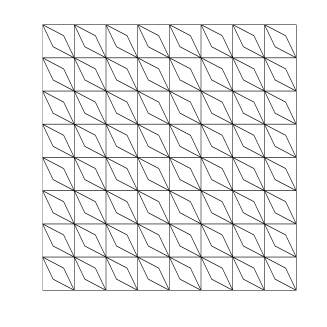
Figure 1: Sample meshes: $\mathcal{T}_{h}^{1}$ (top left), $\mathcal{T}_{h}^{2}$ (top right), $\mathcal{T}_{h}^{3}$ (bottom left) and $\mathcal{T}_{h}^{4}$ (bottom right), for $N=8$.

We have chosen two configurations for the computational domain $\Omega$: $\Omega_{S}:=(0,1)\times(0,1)$ and $\Omega_{L}:=(0,1)\times(0,1)\backslash[1/2,1)\times[1/2,1)$. Even though our theoretical analysis has been developed only for clamped plates, we will consider in Section 5.3 other boundary conditions.

In order to compare our results for the buckling problem, we introduce a non-dimensional buckling coefficient, which is defined as:

$$\widehat{\lambda}_{h}^{(j)}:=\frac{\lambda_{h}^{(j)}L}{\pi^{2}},$$ (5.10)

where $L$ is the plate side length.

Moreover, we will consider different in-plane compressive stress $\boldsymbol{\eta}$. More precisely, we will compute the non-dimensional buckling coefficients using the following $\boldsymbol{\eta}$:

$$\boldsymbol{\eta}_{1}:=\begin{pmatrix}1&0\\ 0&1\end{pmatrix},\qquad\boldsymbol{\eta}_{2}:=\begin{pmatrix}1&0\\ 0&0\end{pmatrix},\qquad\boldsymbol{\eta}_{3}:=\begin{pmatrix}0&1\\ 1&0\end{pmatrix}.$$

The physical meaning of the tensors $\boldsymbol{\eta}_{1},\boldsymbol{\eta}_{2}$ and $\boldsymbol{\eta}_{3}$ is illustrated in Figures 2 and 3, respectively.

Figure 2: $\boldsymbol{\eta}_{1}$ (left) correspond to a uniformly compressed plate (in the $x$, $y$ directions) and $\boldsymbol{\eta}_{2}$ (right) correspond to a plate subjected to uniaxial compression (in the $x$ direction).

Figure 3: $\boldsymbol{\eta}_{3}$ correspond to a plate subjected to shear load.

5.1 Clamped square plate.

In this numerical test we compute the non-dimensional buckling coefficients (cf. (5.10)) for a uniformly compressed square plate $\Omega_{S}$. This corresponds to the stress field $\boldsymbol{\eta}_{1}$

We report in Table 1 the four lowest non-dimensional buckling coefficients computed with the virtual element method analyzed in this paper. The polynomial degrees are given by $k=2,3$ and with two different families of meshes and $N=32,64,128$. The table includes orders of convergence as well as accurate values extrapolated by means of a least-squares fitting. In the last row of the table, we show the values obtained by extrapolating those computed with different method presented in [38].

Table 1: Lowest non-dimensional buckling coefficients $\widehat{\lambda}_{h}^{i}$, $i=1,2,3,4$ of a clamped square plate subjected to a plane stress field $\boldsymbol{\eta}_{1}$.

Mesh	$k$	$N$	$\widehat{\lambda}_{h}^{1}$	$\widehat{\lambda}_{h}^{2}$	$\widehat{\lambda}_{h}^{3}$	$\widehat{\lambda}_{h}^{4}$
		$32$	5.2724	9.1716	9.2744	12.8252
		$64$	5.2952	9.2906	9.3174	12.9461
$\mathcal{T}_{h}^{2}$	2	$128$	5.3014	9.3229	9.3297	12.9786
		Order	1.86	1.88	1.80	1.89
		Extrap.	5.3038	9.3350	9.3347	12.9907
		$32$	5.3037	9.3345	9.3347	12.9918
		$64$	5.3036	9.3342	9.3342	12.9904
$\mathcal{T}_{h}^{2}$	3	$128$	5.3036	9.3342	9.3342	12.9904
		Order	3.95	3.95	3.94	3.93
		Extrap.	5.3036	9.3342	9.3342	12.9903
		$32$	5.3192	9.3581	9.3968	13.0934
		$64$	5.3075	9.3401	9.3498	13.0162
$\mathcal{T}_{h}^{4}$	$2$	$128$	5.3046	9.3356	9.3381	12.9968
		Order	2.00	2.00	2.00	1.99
		Extrap.	5.3036	9.3342	9.3341	12.9903
		$32$	5.3039	9.3348	9.3353	12.9939
		$64$	5.3036	9.3342	9.3342	12.9906
$\mathcal{T}_{h}^{4}$	$3$	$128$	5.3036	9.3342	9.3342	12.9904
		Order	3.94	3.93	3.93	3.91
		Extrap.	5.3036	9.3342	9.3342	12.9903
[38]			5.3037	9.3337	9.3337	12.9909

In this case, since $\Omega_{S}$ is convex, the problem have smooth eigenfunctions, as a consequence, when using degree $k$, the order of convergence is $2(k-1)$ as the theory predicts (cf. Theorem 4.4). Moreover, the results obtained by the two methods agree perfectly well.

In the next test we compute once again the non-dimensional buckling coefficients (in absolute value) of the same plate as in the previous example, subjected to a uniform shear load. This corresponds to the stress field $\boldsymbol{\eta}_{3}$.

In Table 2 we report the four lowest non-dimensional buckling coefficients (in absolute value) considering the stress field $\boldsymbol{\eta}_{3}$. Once again, the polynomial degrees are given by $k=2,3$ and with two different families of meshes and $N=32,64,128$. The table includes orders of convergence as well as accurate values extrapolated by means of a least-squares fitting. In the last row of the table, we show the values obtained by extrapolating those computed with different method presented in [38].

Once again, it can be clearly observed from Table 2 that our method computes the scaled buckling coefficients (cf.(5.10)) with an optimal order of convergence and that the agreement with the method from [38] is excellent.

Table 2: Lowest non-dimensional buckling coefficients (in absolute value) $\widehat{\lambda}_{h}^{i}$, $i=1,2,3,4$ of a clamped square plate subjected to a plane stress tensor field $\boldsymbol{\eta}_{3}$.

Mesh	$k$	$N$	$\widehat{\lambda}_{h}^{1}$	$\widehat{\lambda}_{h}^{2}$	$\widehat{\lambda}_{h}^{3}$	$\widehat{\lambda}_{h}^{4}$
		$32$	14.6083	16.8405	33.2148	35.2101
		$64$	14.6331	16.8983	33.3053	35.2700
$\mathcal{T}_{h}^{1}$	2	$128$	14.6397	16.9137	33.3319	35.2888
		Order	1.89	1.92	1.77	1.67
		Extrap.	14.6422	16.9191	33.3429	35.2974
		$32$	14.6470	16.9242	33.3795	35.3423
		$64$	14.6423	16.9192	33.3437	35.2986
$\mathcal{T}_{h}^{1}$	3	$128$	14.6420	16.9189	33.3413	35.2957
		Order	3.93	3.95	3.90	3.89
		Extrap.	14.6420	16.9188	33.3411	35.2954
		$36$	14.6330	16.9071	33.2479	35.1883
		$64$	14.6398	16.9159	33.3178	35.2685
$\mathcal{T}_{h}^{3}$	2	$128$	14.6415	16.9181	33.3353	35.2887
		Order	2.02	2.01	1.99	1.99
		Extrap.	14.6420	16.9188	33.3412	35.2955
		$32$	14.6455	16.9214	33.3536	35.3098
		$64$	14.6423	16.9190	33.3421	35.2966
$\mathcal{T}_{h}^{3}$	3	$128$	14.6420	16.9189	33.3412	35.2955
		Order	3.63	3.71	3.65	3.62
		Extrap.	14.6420	16.9188	33.3411	35.2954
[38]			14.6420	16.9195	33.3376	-

We show in Figure 4 the buckling mode associated with the lowest scaled buckling coefficient.

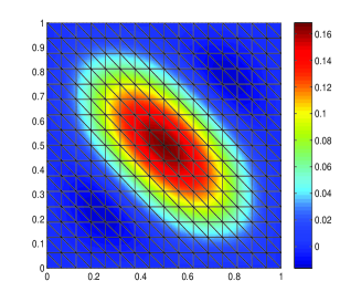
Figure 4: Test 1. Buckling mode associated to the first non-dimensional buckling coefficient of a square plate subjected to a plane stress tensor field $\boldsymbol{\eta}_{3}$.

5.2 Clamped L-shaped plate.

In this numerical test, we consider an L-shaped domain: $\Omega_{L}$. We have used triangular and concave meshes as those shown in $\mathcal{T}_{h}^{3}$ and $\mathcal{T}_{h}^{4}$, respectively (see Figure 1). Once again, the refinement parameter $N$ is the number of elements on each edge.

Table 3 reports the four lowest non-dimensional buckling coefficient computed with the method analyzed in this paper with polynomial degree $k=2$. We include in this table orders of convergence, as well as accurate values extrapolated by means of a least-squares fitting again. In the last row of the table, we show the values obtained by extrapolating those computed with different method presented in [38].

Table 3: Four lowest non-dimensional buckling coefficient of a clamped L-shaped plate and subjected to a plane stress tensor field $\boldsymbol{\eta}_{1}$.

Mesh	$k$	$N$	$\widehat{\lambda}_{1h}$	$\widehat{\lambda}_{2h}$	$\widehat{\lambda}_{3h}$	$\widehat{\lambda}_{4h}$
		$32$	13.1749	15.0809	17.0798	19.9445
		$64$	13.0847	15.0234	17.0203	19.8758
$\mathcal{T}_{h}^{3}$	2	$128$	13.0495	15.0083	17.0042	19.8582
		Order	1.36	1.93	1.89	1.97
		Extrap.	13.0271	15.0029	16.9983	19.8522
		$32$	13.1949	15.1399	17.1801	20.1590
		$64$	13.0903	15.0388	17.0453	19.9297
$\mathcal{T}_{h}^{4}$	2	$128$	13.0511	15.0124	17.0105	19.8717
		Order	1.41	1.94	1.95	1.98
		Extrap.	13.0274	15.0031	16.9983	19.8519
		[38]	13.0290	15.0036	16.9949	-

We observe that for the lowest non-dimensional buckling coefficient, the method converges with order close to $1.089$, which is the expected one because of the singularity of the solution (see [30]). For the other non-dimensional buckling coefficients, the method converges with larger orders.

We show in Figure 5 the buckling mode associated with the lowest scaled buckling coefficient.

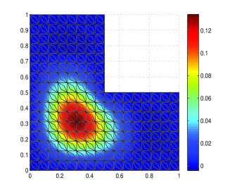
Figure 5: Test 2. Buckling mode associated to the first non-dimensional buckling coefficient of a clamped L-shaped plate subjected to a plane stress tensor field $\boldsymbol{\eta}_{1}$.

5.3 Simply supported-free square plate.

In this final test, which is not covered by our theory since our theoretical results has been developed only for clamped plates, we have computed the non-dimensional buckling coefficient of a simply supported-free square plate, subjected to linearly varying in-plane load in one direction ($x$ direction). This corresponds to a plane stress field given by

$$\widetilde{\boldsymbol{\eta}}_{2}:=\begin{pmatrix}1-\alpha\frac{y}{L}&0\\ 0&0\end{pmatrix},$$ (5.11)

with values of $\alpha$ in $\{0,2/3,1,4/3,2\}$. We observe that for $\alpha=0$, we obtain the plane stress tensor field $\boldsymbol{\eta}_{2}$.

We take an square plate $\Omega_{S}$ which has two simply supported edges and two free edges.

We report in Table 4 the non-dimensional buckling coefficient. The polynomial degrees are given by $k=2,3$ and the family of meshes $\mathcal{T}_{h}^{2}$ with $N=32,64,128$. The table includes computed orders of convergence and extrapolated more accurate values of each eigenvalue obtained by means of a least-squares fitting.

Table 4: Non-dimensional buckling coefficient $\widehat{\lambda}_{1h}$ for different values of $\alpha$ of a square plate with mixed boundary conditions and subjected to linearly varying in-plane load in one direction $\widetilde{\boldsymbol{\eta}}_{2}$.

Mesh	$k$	$N$	$\alpha=0$	$\alpha=2/3$	$\alpha=1$	$\alpha=4/3$	$\alpha=2$
		32	0.9984	1.4474	1.7763	2.1687	3.0676
		64	0.9996	1.4490	1.7782	2.1709	3.0702
$\mathcal{T}_{h}^{2}$	2	128	0.9999	1.4495	1.7787	2.1715	3.0710
		Order	1.91	1.90	1.90	1.88	1.85
		Extrap.	1.0000	1.4496	1.7789	2.1717	3.0713
		32	1.0000	1.4496	1.7789	2.1717	3.0712
		64	1.0000	1.4496	1.7789	2.1717	3.0712
$\mathcal{T}_{h}^{2}$	3	128	1.0000	1.4496	1.7789	2.1717	3.0712
		Order	4.00	4.00	4.00	4.00	4.00
		Extrap.	1.0000	1.4496	1.7789	2.1717	3.0712

It can be clearly observed from Table 4 that the proposed virtual scheme computes the scaled buckling coefficient (cf. (5.10)) with an optimal order of convergence for all the values of $\alpha$.

Finally, we show in Figure 6 the buckling mode associated with the lowest scaled buckling coefficient for different values of the parameter $\alpha$.

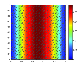
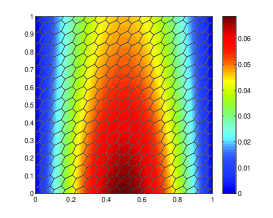
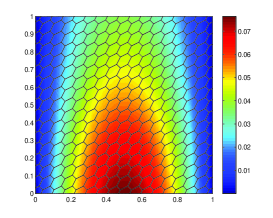
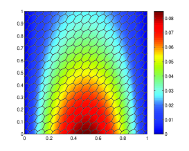
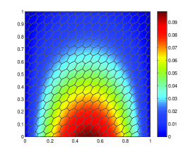
Figure 6: Test 3. Buckling modes associated to the first non-dimensional buckling coefficient $\widehat{\lambda}_{1h}$ of a square plate with mixed boundary conditions and subjected to linearly varying in-plane load in one direction $\widetilde{\boldsymbol{\eta}}_{2}$ (cf. (5.11)): $\alpha=0$ (top left), $\alpha=2/3$ (top middle), $\alpha=1$ (top right), $\alpha=4/3$ (bottom left), $\alpha=2$ (bottom right).

References

- [1] B. Ahmad, A. Alsaedi, F. Brezzi, L. D. Marini and A. Russo, Equivalent projectors for virtual element methods, Comput. Math. Appl., 66, (2013), pp. 376–391.
- [2] P.F. Antonietti, L. Beirão da Veiga, D. Mora and M. Verani, A stream virtual element formulation of the Stokes problem on polygonal meshes, SIAM J. Numer. Anal., 52, (2014), pp. 386–404.
- [3] P.F. Antonietti, L. Beirão da Veiga, S. Scacchi and M. Verani, A virtual element method for the Cahn–Hilliard equation with polygonal meshes, SIAM J. Numer. Anal., 54, (2016), pp. 36–56.
- [4] E. Artioli, S. de Miranda, C. Lovadina and L. Patruno, A family of virtual element methods for plane elasticity problems based on the Hellinger-Reissner principle, Comput. Methods Appl. Mech. Engrg., 340, (2018), pp. 978–999.
- [5] I. Babuška and J. Osborn, Eigenvalue problems, in Handbook of Numerical Analysis, Vol. II, P.G. Ciarlet and J.L. Lions, eds., North-Holland, Amsterdam, 1991, pp. 641–787.
- [6] L. Beirão da Veiga, F. Brezzi, A. Cangiani, G. Manzini, L.D. Marini and A. Russo, Basic principles of virtual element methods, Math. Models Methods Appl. Sci., 23, (2013), pp. 199–214.
- [7] L. Beirão da Veiga, F. Brezzi, F. Dassi, L.D. Marini and A. Russo, Virtual Element approximation of 2D magnetostatic problems, Comput. Methods Appl. Mech. Engrg., 327, (2017) pp. 173–195.
- [8] L. Beirão da Veiga, F. Brezzi, F. Dassi, L.D. Marini and A. Russo, Lowest order Virtual Element approximation of magnetostatic problems, Comput. Methods Appl. Mech. Engrg., 332, (2018) pp. 343–362.
- [9] L. Beirão da Veiga, F. Brezzi and L.D. Marini, Virtual elements for linear elasticity problems, SIAM J. Numer. Anal., 51 (2013), pp. 794–812.
- [10] L. Beirão da Veiga, F. Brezzi, L.D. Marini and A. Russo, The hitchhiker’s guide to the virtual element method, Math. Models Methods Appl. Sci., 24, (2014), pp. 1541–1573.
- [11] L. Beirão da Veiga, C. Lovadina and D. Mora, A virtual element method for elastic and inelastic problems on polytope meshes, Comput. Methods Appl. Mech. Engrg., 295, (2015) pp. 327–346.
- [12] L. Beirão da Veiga, C. Lovadina and G. Vacca, Divergence free virtual elements for the Stokes problem on polygonal meshes, ESAIM Math. Model. Numer. Anal., 51, (2017), pp. 509–535.
- [13] L. Beirão da Veiga, D. Mora and G. Rivera, Virtual elements for a shear-deflection formulation of Reissner-Mindlin plates, Math. Comp., 88, (2019), pp. 149–178.
- [14] L. Beirão da Veiga, D. Mora, G. Rivera and R. Rodríguez, A virtual element method for the acoustic vibration problem, Numer. Math., 136, (2017), pp. 725–763.
- [15] M.F. Benedetto, S. Berrone, A. Borio, S. Pieraccini and S. Scialò, Order preserving SUPG stabilization for the virtual element formulation of advection–diffusion problems, Comput. Methods Appl. Mech. Engrg., 311, (2016), pp. 18–40.
- [16] S.C. Brenner, Q. Guan and L.-Y Sung, Some estimates for virtual element methods, Comput. Methods Appl. Math., 17, (2017), pp. 553–574.
- [17] S.C. Brenner, P. Monk and J. Sun, C0 interior penalty Galerkin method for biharmonic eigenvalue problems, in Spectral and High Order Methods for Partial Differential Equations. Lect. Notes Comput. Sci. Eng., 106, (2015), pp. 3–15.
- [18] S.C. Brenner and R.L. Scott, The Mathematical Theory of Finite Element Methods, Springer, New York, 2008.
- [19] F. Brezzi and L.D. Marini, Virtual elements for plate bending problems, Comput. Methods Appl. Mech. Engrg., 253, (2013), pp. 455–462.
- [20] J. Cao, Z. Wang, W. Cao and L. Chen, A mixed Legendre-Galerkin spectral method for the buckling problem of simply supported Kirchhoff plates, Bound. Value Probl., 34, (2017), pp. 1–12
- [21] E. Cáceres and G.N. Gatica, A mixed virtual element method for the pseudostress-velocity formulation of the Stokes problem, IMA J. Numer. Anal., 37, (2017), pp. 296–331.
- [22] E. Cáceres, G.N. Gatica and F. Sequeira, A mixed virtual element method for the Brinkman problem, Math. Models Methods Appl. Sci., 27, (2017) pp. 707–743.
- [23] A. Cangiani, G. Manzini and O.J. Sutton, Conforming and nonconforming virtual element methods for elliptic problems, IMA J. Numer. Anal., 37, (2017), pp. 1317–1354.
- [24] C. Chinosi and L.D. Marini, Virtual element method for fourth order problems: -estimates, Comput. Math. Appl., 72, (2016), pp. 1959–1967.
- [25] P.G. Ciarlet, The Finite Element Method for Elliptic Problems, SIAM, 2002.
- [26] Ö. Civalek, A. Korkmazb and Ç. Demir, Discrete singular convolution approach for buckling analysis of rectangular Kirchhoff plates subjected to compressive loads on two-opposite edges, Adv. Eng. Softw., 41, (2010), pp. 557–560.
- [27] F. Gardini, G. Manzini and G. Vacca, The nonconforming virtual element method for eigenvalue problems, arXiv:1802.02942 [math.NA], (2018), to appear in ESAIM Math. Model. Numer. Anal.
- [28] F. Gardini and G. Vacca, Virtual element method for second-order elliptic eigenvalue problems, IMA J. Numer. Anal., 38, (2018), pp. 2026–2054.
- [29] V. Girault and P.A. Raviart, Finite Element Methods for Navier-Stokes Equations, Springer-Verlag, Berlin, 1986.
- [30] P. Grisvard, Elliptic Problems in Non-Smooth Domains, Pitman, Boston, 1985.
- [31] P. Hansbo and M.G. Larson, A posteriori error estimates for continuous/discontinuous Galerkin approximations of the Kirchhoff-Love buckling problem, Comput. Mech., 56, (2015), pp. 815–827.
- [32] K. Ishihara, On the mixed finite element approximation for the buckling of plates, Numer. Math., 33, (1979), pp. 195–210.
- [33] L. Mascotto, I. Perugia and A. Pichler, Non-conforming harmonic virtual element method: - and - versions, J. Sci. Comput., 77, (2018), pp. 1874–1908.
- [34] F. Millar and D. Mora, A finite element method for the buckling problem of simply supported Kirchhoff plates, J. Comp. Appl. Math., 286, (2015), pp. 68–78.
- [35] D. Mora and G. Rivera, A priori and a posteriori error estimates for a virtual element spectral analysis for the elasticity equations, IMA J. Numer. Anal., DOI: https://doi.org/10.1093/imanum/dry063 (2019).
- [36] D. Mora, G. Rivera and R. Rodríguez, A virtual element method for the Steklov eigenvalue problem, Math. Models Methods Appl. Sci., 25, (2015), pp. 1421–1445.
- [37] D. Mora, G. Rivera and I. Velásquez, A virtual element method for the vibration problem of Kirchhoff plates, ESAIM Math. Model. Numer. Anal., 52, (2018), pp. 1437–1456.
- [38] D. Mora and R. Rodríguez, A piecewise linear finite element method for the buckling and the vibration problems of thin plates, Math. Comp., 78, (2009), pp. 1891–1917.
- [39] D. Mora and I. Velásquez, A virtual element method for the transmission eigenvalue problem, Math. Models Methods Appl. Sci., 28, (2018), pp. 2803–2831.
- [40] I. Perugia, P. Pietra and A. Russo, A plane wave virtual element method for the Helmholtz problem, ESAIM Math. Model. Numer. Anal., 50, (2016), pp. 783–808.
- [41] R. Rannacher, Nonconforming finite element methods for eigenvalue problems in linear plate theory, Numer. Math., 33, (1979), pp. 23–42.
- [42] S.P. Timoshenko and J.M. Gere, Theory of Elastic Stability, McGraw-Hill, New York, 1961.
- [43] G. Vacca, An -conforming virtual element for Darcy and Brinkman equations, Math. Models Methods Appl. Sci., 28, (2018), pp. 159–194.
- [44] P. Wriggers, W.T. Rust and B.D. Reddy, A virtual element method for contact, Comput. Mech., 58, (2016), pp. 1039–1050.