An evolving and mass dependent - relation for galaxies.
Abstract
The scatter () of the specific star formation rates (sSFRs) of galaxies is a measure of the diversity in their star formation histories (SFHs) at a given mass. In this paper we employ the EAGLE simulations to study the dependence of the of galaxies on stellar mass () through the - relation in . We find that the relation evolves with time, with the dispersion depending on both stellar mass and redshift. The models point to an evolving U-shape form for the - relation with the scatter being minimal at a characteristic mass of and increasing both at lower and higher masses. This implication is that the diversity of SFHs increases towards both at the low- and high-mass ends. We find that active galactic nuclei feedback is important for increasing the for high mass objects. On the other hand, we suggest that SNe feedback increases the of galaxies at the low-mass end. We also find that excluding galaxies that have experienced recent mergers does not significantly affect the - relation. Furthermore, we employ the combination of the EAGLE simulations with the radiative transfer code SKIRT to evaluate the effect of SFR/stellar mass diagnostics in the - relation and find that the methodologies (e.g. SED fitting, UV+IR, UV+IRX-) widely used in the literature to obtain intrinsic properties of galaxies have a large effect on the derived shape and normalization of the - relation.
1 Introduction
The scatter ( ) of the specific star formation rate (the ratio of star formation rate and stellar mass)-stellar mass () relation provides a measurement for the variation of star formation across galaxies of similar masses with physical mechanisms important for galaxy evolution make their imprint to it. These processes include gas accretion, minor mergers, disc dynamics, halo heating, stellar feedback and AGN feedback. The above are typically dependent on galaxy stellar mass and cosmic epoch (Cano-Díaz et al., 2016; Abbott et al., 2017; Wang et al., 2017; Chiosi et al., 2017; García et al., 2017; Eales et al., 2018; Qin et al., 2018; Sánchez et al., 2018; Cañas et al., 2018; Blanc et al., 2019) and possibly affect the shape of the - differently. However, it is difficult to study and especially quantify the effect of the different prescriptions important for galaxy evolution to the scatter solely by using insights from observations.
In addition, the shape of the - relation and the value of the dispersion is a matter of debate in the literature. The scatter is usually reported to be constant ( dex) with stellar mass in most studies, especially those which address the high and intermediate redshift Universe (). For example, Rodighiero et al. (2010) and Schreiber et al. (2015), using mostly UV-derived SFRs, suggest that the dispersion is independent on galaxy mass and constant ( dex) over a wide range for star forming galaxies ( ). Whitaker et al. (2012) reported a variation of 0.34 dex from Spitzer MIPS observations. Similarly, Noeske et al. (2007) and Elbaz et al. (2007) reported a 1 dispersion in of around dex at for their flux-limited sample. However, other studies suggest that the dispersion tends to be larger for more massive objects and in the lower-redshift Universe (Guo et al., 2013; Ilbert et al., 2015) implying that mechanisms important for galaxy evolution are prominent and contribute to a variety of star formation histories for massive galaxies. On the other hand, Santini et al. (2017) suggested that the scatter decreases with increasing mass and this implies that mechanisms important for galaxy formation are giving a larger diversity of SFHs to low mass objects. In addition, Boogaard et al. (2018) using the MUSE Hubble Ultra Deep Field Survey suggest that the intrinsic scatter of the relation at the low mass end is dex and larger than what is typically found at higher masses. In disagreement with all the above, Willett et al. (2015) using the Galaxy Zoo survey for find a dispersion that actually decreases with mass at from dex to dex and increases again at to reach a scatter of dex. All the above observational studies have conflicting results and this is possibly because they are affected by selection effects, uncertainties originating from star formation rate diagnostics (Katsianis et al., 2016; Davies et al., 2017), different separation criteria for passive/star forming galaxies (Renzini & Peng, 2015) and usually focus on different redshifts and masses. In addition, the observed scatter can be different than the intrinsic value. More specifically, at the high-mass end an increased scatter can be inferred due to the uncertainties in removing passive objects, while at the low-mass end an increased scatter can be due to poor signal-to-noise ratio 111According to Kurczynski et al. (2016) the intrinsic scatter is / dex lower than the observed value at /.. Due to the above conflicting results and limitations it is almost impossible to decipher if there is an evolution in the scatter of the relation and if it is mass/redshift dependent or not, solely by relying on observations.
Cosmological simulations are able to reproduce realistic star formation rates and stellar masses of galaxies (Tescari et al., 2014; Katsianis et al., 2015; Furlong et al., 2015; Katsianis et al., 2017b; Pillepich et al., 2018) and thus are a valuable tool to address the questions related to the shape of the -, the value of the dispersion, and the way mechanisms important to galaxy evolution affect it. Simulations have limitations in resolution and box size. Thus they suffer from small number statistics of galaxies at a given mass, especially at the high-stellar mass end and cosmic variance due to finite box-size. However, despite their limitations the retrieved properties of galaxies do not suffer from poor S/N at the low mass end or uncertainties brought by different methodologies employed in observational studies (Katsianis et al., 2016, 2017a) and thus can provide a useful guide to future surveys or address controversies in galaxy formation Physics. Dekel et al. (2009) pointed out that the scatter of the specific star formation rate - stellar mass relation in cosmological simulations is about 0.3 dex and driven mostly by the galaxies’ gas accretion rates. Hopkins et al. (2014) using the FIRE zoom-in cosmological simulations studied the dispersion in the SFR smoothed over various time intervals and pointed out that the star formation main sequence and distribution of specific SFRs emerge naturally from the shape of the galaxies’ star formation histories, from at . The authors suggested that the scatter is larger on small timescales and masses, while dwarf galaxies () exhibit much more bursty SFHs (and therefore larger scatter) due to stochastic processes like star cluster formation, and their associated feedback. Matthee & Schaye (2018) argued that the scatter of the main sequence - relation, defined by a sSFR cut in galaxies, is mass dependent and decreasing with mass at , while presenting a comparison between the EAGLE reference model and SDSS data. The authors suggested that the scatter of the relation originates from a combination of fluctuations on short time-scales (ranging from 0.2-2 Gyr) that are presumably associated with self-regulation from cooling, star formation and outflows (which nature is stochastic), but is dominated by long time-scale variations (Hopkins et al., 2014; Torrey et al., 2017), which is governed by the SFHs of galaxies, especially at high masses (222The authors pointed out that the total scatter of is driven by a combination of short and long time-scale variations, while for massive galaxies () the contribution of stochastic fluctuations (Kelson, 2014) is not significant ( 0.1 dex). For objects with the contribution of fluctuations on short time scales, which nature is more stochastic, becomes relatively more important ( 0.2 dex).. Dutton et al. (2010) using a semi-analytic model suggested that the scatter of the SFR sequence appears to be invariant with redshift and with a small value of dex.
The Virgo project Evolution and Assembly of GaLaxies and their Environments simulations (EAGLE, Schaye et al., 2015; Crain et al., 2015) is a suite of cosmological hydrodynamical simulations in cubic, periodic volumes ranging from 25 to 100 comoving Mpc per side. The reference model reproduces the observed star formation rates of galaxies (Katsianis et al., 2017b) and the evolution of the stellar mass function (Furlong et al., 2015). In addition, EAGLE allows us to investigate this problem with superb statistics (several thousands of galaxies at each redshift) and investigate different configurations that include different subgrid Physics. All the above provide a powerful resource for understanding the - relation, address the shortcomings of observations, study its evolution across cosmic time and decipher its shape.
In this paper, we examine the dependence of the sSFR dispersion on using the EAGLE simulations (Schaye et al., 2015; Crain et al., 2015; Katsianis et al., 2017b). In section 2 we present the simulations used for this work. In section 3 we discuss the evolution of the - relation (subsection 3.1 presents the reference model) and how different feedback prescriptions (subsection 3.2) and ongoing mergers (subsection 3.3) affect its shape. In addition, we employ the EAGLE+SKIRT data (Camps et al., 2018), which represent a post-process of the simulations with the radiative transfer code SKIRT, in order to decipher how star formation rate and stellar mass diagnostics affect the relation in section 4. Finally in section 5 we draw our conclusions. Studies of the dispersion that rely solely on 2d scatter plots (i.e. displays of the location of the individual sources in the plane) are not able to provide a quantitative information of how galaxies are distributed around the mean sSFR and cannot account for galaxies that could be under-sampled or missed by selection effects so we extend our analysis of the dispersion of the sSFRs at different mass intervals on their distribution/histogram, namely the specific Star Formation Rate Function (sSFRF) by comparing the results of EAGLE with the observations present in Ilbert et al. (2015). In appendix A we present the evolution of the simulated specific star formation rate function in order to present how the sSFRs are distributed.
2 The EAGLE simulations used for this work
The EAGLE simulations track the evolution of baryonic gas, stars, massive black holes and non-baryonic dark matter particles from a starting redshift of down to . The different runs were performed to investigate the effects of resolution, box size and various physical prescriptions (e.g. feedback and metal cooling). For this work we employ the reference model (L100N1504-Ref), a configuration with smaller boxsize (50 Mpc) but same resolution and physical prescriptions (L50N752-Ref), a run without AGN feedback (L50N752-NoAGN) and a simulation without SN feedback but AGN included (L50N752-OnlyAGN). We outline a summary of the different configurations in Table 1.
| Run | L [Mpc] | NTOT | Feedback |
|---|---|---|---|
| L100N1504-Ref | 100 | 2 | AGN SN |
| L100N1504-Ref+SKIRT | 100 | 2 | AGN SN |
| L50N752-Ref | 50 | 2 | AGN SN |
| L50N752-NoAGN | 50 | 2 | No AGN SN |
| L50N752-OnlyAGN | 50 | 2 | AGN No SN |
Note. — Summary of the different EAGLE simulations used in this work. Column 1, run name; column 2, Box size of the simulation in comoving Mpc; column 3, total number of particles (N NGAS NDM with NGAS NDM); column 4, combination of feedback implemented; The mass of the dark matter particle mDM is 9.70 [], the mass of the initial mass of the gas particle mgas is 1.81 [] and the comoving gravitational softening length is 2.66 in KPc in all configurations.
The EAGLE reference simulation has particles (an equal number of gas and dark matter elements) in an L = 100 comoving Mpc volume box, initial gas particle mass of , and mass of dark matter particles of . The simulations were run using an improved and updated version of the N-body TreePM smoothed particle hydrodynamics code GADGET-3 (Springel, 2005) and employ the star formation recipe of Schaye & Dalla Vecchia (2008). In this scheme, gas with densities exceeding the critical density for the onset of the thermo-gravitational instability () is treated as a multi-phase mixture of cold molecular clouds, warm atomic gas and hot ionized bubbles which are all approximately in pressure equilibrium (Schaye, 2004). The above mixture is modeled using a polytropic equation of state , where P is the gas pressure, is the gas density and is a constant which is normalized to at the density threshold which marks the onset of star formation. The simulations adopt the stochastic thermal feedback scheme described in Dalla Vecchia & Schaye (2012). In addition to the effect of re-heating interstellar gas from star formation, which is already accounted for by the equation of state, galactic winds produced by Type II Supernovae are also considered. EAGLE models AGN feedback by seeding galaxies with BHs as described by Springel (2005), where seed BHs are placed at the center of every halo more massive than M that does not already contain a BH. When a seed is needed to be implemented at a halo, its highest density gas particle is converted into a collisionless BH particle inheriting the particle mass. These BHs grow by accretion of nearby gas particles or through mergers. A radiative efficiency of is assumed for the AGN feedback. Other prescriptions such as inflow-induced starbursts, stripping of gas due to different interactions between galaxies, stochastic IMF sampling or variations to the AGN feedback prescription such as torque-driven accretion models (Anglés-Alcázar et al., 2017) or kinetic feedback (Weinberger et al., 2017) are not currently modeled in EAGLE. The EAGLE reference model and its feedback prescriptions have been calibrated to reproduce key observational constraints, into the present-day stellar mass function of galaxies (Li & White, 2009; Baldry et al., 2012), the correlation between the black hole and bulge masses (McConnell & Ma, 2013) and the dependence of galaxy sizes on mass (Baldry et al., 2012) at . Alongside with these observables the simulation was able to match many other key properties of galaxies in different eras, like molecular hydrogen abundances (Lagos et al., 2015), colors and luminosities at (Trayford et al., 2015), supermassive black hole mass function (Rosas-Guevara et al., 2016), angular momentum evolution (Lagos et al., 2017), atomic hydrogen abundances (Crain et al., 2017), sizes (Furlong et al., 2017), SFRs (Katsianis et al., 2017b), Large-scale outflows (Tescari et al., 2018) and ring galaxies (Elagali et al., 2018). In addition, Schaller et al. (2015) pointed out that there is a good agreement between the normalization and slope of the main sequence present in Chang et al. (2015) and the EAGLE reference model. Katsianis et al. (2016) demonstrated that cosmological hydrodynamic simulations like EAGLE, Illustris (Sparre et al., 2015) and ANGUS (Tescari et al., 2014) produce very similar results for the SFR- relation with a normalization being in agreement with that found in observations at (Kajisawa et al., 2010; De Los Reyes et al., 2014; Bauer et al., 2013; Salmon et al., 2015) and a slope close to unity. In this work, galaxies and their host halos are identified by a friends-of-friends (FoF) algorithm (Davis et al., 1985) followed by the SUBFIND algorithm (Springel et al., 2001; Dolag & Stasyszyn, 2009) which is used to identify substructures or subhalos across the simulation. The star formation rate of each galaxy is defined to be the sum of the star formation rate of all gas particles that belong to the corresponding subhalo and that are within a 3D aperture with radius 30 kpc (Schaye et al., 2015; Crain et al., 2015; Katsianis et al., 2017b).
| z | 0 | 0.350 | 0.615 | 0.865 | 1.400 | 2.000 | 3.000 | 4.000 |
|---|---|---|---|---|---|---|---|---|
| - sSFR Cut () | ||||||||
| , | 0.08 | 0.06 | 0.10 | 0.07 | 0.04 | 0.08 | 0.08 | 0.05 |
| , | 0.12 | 0.10 | 0.09 | 0.07 | 0.04 | 0.08 | 0.12 | 0.09 |
| , | 0.32 | 0.24 | 0.37 | 0.32 | 0.27 | 0.33 | 0.35 | 0.29 |
| - sSFR Cut () | Guo et al. (2015) | |||||||
| , | 0.02 | 0.03 | 0.02 | 0.03 | 0.02 | 0.02 | 0.01 | 0.01 |
| , | 0.03 | 0.05 | 0.03 | 0.02 | 0.01 | 0.01 | 0.01 | 0.01 |
| , | 0.17 | 0.16 | 0.17 | 0.10 | 0.04 | 0.02 | 0.01 | 0.01 |
Note. — The fraction of passive galaxies () at each redshift excluded in order to define a main sequence. We adopt the effect of two different sSFR cuts. The first criterion (Furlong et al., 2015; Matthee & Schaye, 2018) is used to define the - relation, while the second, more moderate criterion (Ilbert et al., 2015; Guo et al., 2015) is used to define the - relation.
| Publication | Redshift range | Technique to obtain | Uncertainty, with [dex] | ||
|---|---|---|---|---|---|
| Stellar mass range | sSFRs and SFRs | Intrinsic or Observed , Shape of - | |||
| Noeske et al. (2007) | z = 0.32, 0.59, 1.0 | EL+UV+ | 0.3 [0.3 0.3] | ||
| Observed, Constant | |||||
| Rodighiero et al. (2010) | z = 1.47, 2.2 | UV+ | 0.3 [0.3 0.3] | ||
| Observed, Constant | |||||
| Guo et al. (2013) | z = 0.7 | UV+ | 0.24 [0.182 0.307] | ||
| Observed, increases with | |||||
| Schreiber et al. (2015) | z = 0.5, 1.0, 1.5, 2.2, 3.0 | 0.35 [0.29 0.37] | |||
| Observed, increases with | |||||
| Ilbert et al. (2015) | z = 0.3, 0.7, 0.9, 1.3, | 0.33 [0.22 0.481] | |||
| Observed, increases with | |||||
| Willett et al. (2015) | z | 0.33 [0.52 0.37 0.48] | |||
| Observed, U-Shape | |||||
| Guo et al. (2015) | 0.44 [0.366 0.557] | ||||
| Observed, increases with | |||||
| Kurczynski et al. (2016) | z = 0.75, 1.25, 1.75, 2.25, 2.75 | SED fitting | 0.40 [0.404 0.315 0.435] | ||
| Intrinsic, redshift/mass dependent | |||||
| Santini et al. (2017) | z = 1.65, 2.5, 3.5 | UV + slope | 0.42 [0.54 0.31] | ||
| Observed, decreases with | |||||
| Boogaard et al. (2018) | z = 0.1 - 0.9 | H+H | 0.44 [0.44 0.44] | ||
| Intrinsic, constant | |||||
| Davies et al. (2019) | z 0.1 | 0.66 [0.74308562 0.53393775 0.70720613] | |||
| Observed, U-shape | |||||
| Davies et al. (2019) | z 0.1 | 0.44 [0.42797872 0.3490565 0.53074792] | |||
| Observed, U-Shape |
3 The evolution of the intrinsic - relation
In this section we present the evolution of the - relation in order to quantify and decipher its evolution and its dependence (or not) upon stellar mass and redshift. In subsection 3.1 we present the results of the EAGLE reference model and the compilation of observations used in this work, while in subsections 3.2 and 3.3 we focus on the effect of feedback and mergers on the - relation, respectively. For the simulations, we split the sample of galaxies at each redshift in 30 stellar mass bins from to (stellar mass bins of 0.18 dex at ) and measure the 1 standard deviation in each bin.
We compare our simulated results with a range of observational studies in which usually different authors employ different techniques to exclude quiescent objects in their samples. In order to select only Star Forming Galaxies (SFGs) the authors may select only blue cloud galaxies (Peng et al., 2010), or use the BzK two-color selection (Daddi et al., 2007a), or the standard BPT (Baldwin et al., 1981) criterion, or employ the rest-frame UVJ selection (Whitaker et al., 2012; Schreiber et al., 2015) or an empirical color selection (Rodighiero et al., 2010; Guo et al., 2013; Ilbert et al., 2015) or specify a sSFR separation criterion (Guo et al., 2015). All these criteria should ideally cut out galaxies with low sSFR, but the thresholds differ significantly in value from one study to another, with some being redshift dependent and others not (Renzini & Peng, 2015). In order to surpass this complication and uncertainty of the effectiveness of excluding “passive objects” in observational studies, in the following subsection we present:
-
•
the - of the full (Star forming Passive) EAGLE sample,
- •
- •
The differences between observations used in this work in terms of assumed methodology to exclude (or not) quiescent objects is described in the previous paragraph and table 2. The different data sets and methodologies to obtain SFRs for the same studies are described below and table 3. Noeske et al. (2007) used 2095 field galaxies from the Wavelength Extended Groth Strip International Survey (AEGIS) and derived SFRs from emission lines, GALEX, and Spitzer MIPS and 24m photometry. Guo et al. (2013) used 12,614 objects from the multi-wavelength data set of COSMOS, while SFRs are obtained combining 24 m and UV luminosities. Schreiber et al. (2015) used GOODS-North, GOODS-South, UDS, and COSMOS extragalactic fields and derived SFRs using UV+FIR luminosities. Ilbert et al. (2015) based their analysis on a 24 m selected catalogue combining the COSMOS and GOODS surveys. The authors estimated SFRs by combining mid- and far-infrared data for 20,500 galaxies. Willett et al. (2015) used optical observations in the SDSS DR7 survey, while stellar masses and star formation rates are computed from optical diagnostics and taken from the MPA-JHU catalogue (Salim et al., 2007). Guo et al. (2015) used the SDSS data release 7, while in their studies SFRs are estimated from H in combination with 22 m observation from the Wide-field Infrared Survey Explorer. Santini et al. (2017) used the Hubble Space Telescope Frontier Fields, while SFRs were estimated from observed UV rest-frame photometry (Meurer et al., 1999; Kennicutt & Evans, 2012). Davies et al. (2019) used 9,005 galaxies from the GAMA survey (Driver et al., 2011, 2016a). The SFR indicators used are described in length in Driver et al. (2016b) and involve a) the SED fitting code magphys, b) a combination of Ultraviolet and Total Infrared (UV+TIR), c) H emission line d) the Wide-field Infrared Survey Explorer (WISE) W3-band (Cluver et al., 2017), and e) extinction-corrected u-band luminosities derived using the GAMA rest-frame u -band luminosity and u-g colors.

3.1 The evolution of the -, - and - relations in the EAGLE model
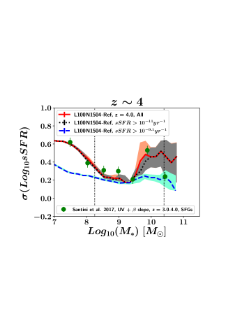
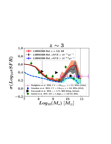
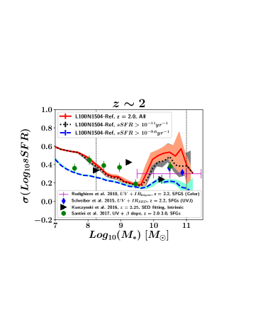
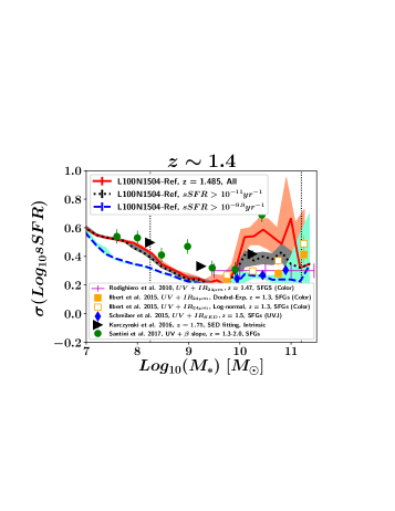
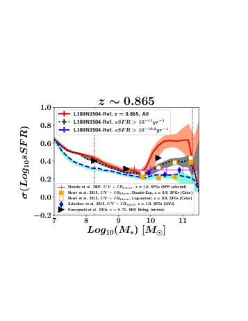
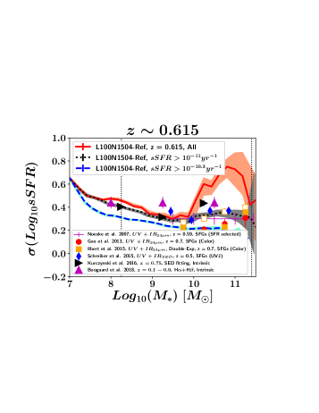
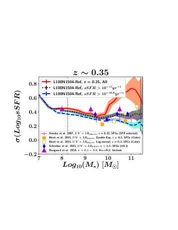
In Fig. 1 we present the evolution of the -, which includes both passive and star forming objects (represented by the red solid line), and the “main sequence” - (represented by the black dotted line) and - (represented by the blue dashed line) relations in the EAGLE L100N1504-Ref at to and compare them with observations. The two vertical dotted lines represent the mass resolution limit of 100 baryonic particles () and the statistic limit where there are fewer than 10 galaxies at the low- and high-mass ends (Furlong et al., 2015; Katsianis et al., 2017b). The shaded regions represent the 95 % bootstrap confidence interval for 5000 re-samples for the - relation.
Starting from redshift (top left panel of Fig. 1) we see that the - of the reference model has a U-shape form. The dispersion decreases with mass at the interval from to dex while it increases with mass at the interval from to dex. For the “main sequence”, - relation, defined by the exclusion of objects with (Furlong et al., 2015; Matthee & Schaye, 2018), the scatter increases more moderately at the high mass end (from 0.2 dex to 0.3 dex), since passive objects which would increase the dispersion are excluded using a sSFR cut. We note that at this era the fraction of quiescent galaxies is expected to be small, thus the exclusion of quiescent objects should not affect significantly the relation (especially at the low mass end), and it is very possible that the above selection criterion is too strict. However, a more moderate cut of (Ilbert et al., 2015) results in a relationship that is closer to that of the full EAGLE sample since the exclusion of quenched objects is less severe. We note that the observations of Santini et al. (2017) are broadly consistent with the - (represented by the black dotted line) and - (represented by the red solid line) relations (green filled circles representing the observations of Santini et al. (2017) within 0.1 dex with respect the simulated results). A similar behavior is found for lower redshifts up to . This is possibly due to the fact that the moderate sSFR cut of (Ilbert et al., 2015) resembles more closely the selection performed by Schreiber et al. (2015) and Santini et al. (2017).
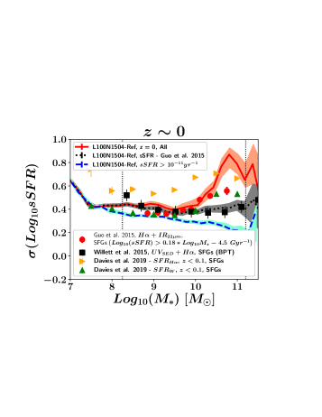
At redshift (left medium panel of Fig. 1) we find that there is an increment of scatter with mass for the EAGLE - and - relations at the high mass end () from dex to and dex, respectively. On the other hand, the - relation has an almost constant scatter of dex with mass at . The observations for this mass interval (Rodighiero et al., 2010; Guo et al., 2013; Ilbert et al., 2015; Schreiber et al., 2015) typically lay between the two “main sequence” relations - and -, something that is possibly related to the uncertainties of removing quiescent objects in the literature (Renzini & Peng, 2015). The observations of Ilbert et al. (2015) and Schreiber et al. (2015) imply an increasing scatter with mass, while those of Noeske et al. (2007) and Rodighiero et al. (2010) a constant ( dex). On the other hand, for the low- mass end () there is a decrement with mass according to the EAGLE reference model in agreement with Santini et al. (2017). Similarly with higher redshifts the - and - relations have a U-shape form. The same behavior is found for lower redshifts up to , which reflects the fact that both low and high mass galaxies have a larger scatter/diversity of star formation histories than (characteristic mass) objects. For (bottom right panel of Fig. 1) the scatter is constant with mass for both the - and - relations for the interval at dex. The scatter increases for the high mass end to dex when both passive and star forming galaxies are included. The increment is more moderate when cuts similar to the ones of Guo et al. (2015) are applied. On the other hand, the scatter decreases with mass for the “ main sequence” - relation from 0.4 dex to 0.2 dex.
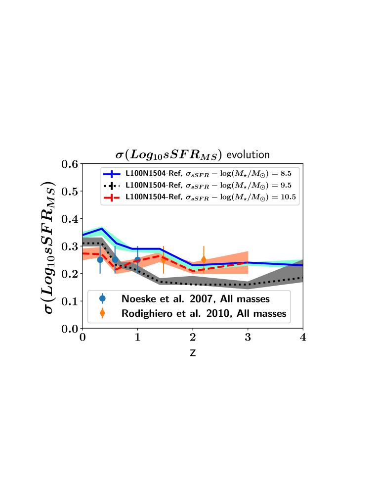
We note that the EAGLE reference model suggests that both - and - relations are evolving with redshift and are not time independent. In Fig. 2 we present the evolution of the at for the stellar masses of (blue solid line), (black dotted line) and (red dashed line). The blue circles, black squares and red triangles represent the compilation of observations of (Guo et al., 2013; Ilbert et al., 2015; Schreiber et al., 2015; Willett et al., 2015; Santini et al., 2017) at , and , respectively. Both in simulations and observations the at increases steadily from 0.33 dex at to 0.55 dex. For the scatter remains almost constant at dex for but increases up to 0.35 at for the redshift interval of . Last, the scatter increases from 0.25 dex to 0.45 dex at .
In Fig. 3 we present the evolution of the at for the stellar masses of (blue solid line), (black dotted line) and (red dashed line). The scatter increases at from dex to dex at and from dex to dex at . However, the remains almost constant at dex at .
In conclusion, the - relation (represented by the red solid line) has a U-shape form at all redshifts with the scatter typically decreasing at the mass interval and increasing at . This implies a diversity of star formation histories for both the low and high mass ends. The above is supported by recent observations, while a complementary work using data from the GAMA survey demonstrates as well the U-shape form of the - relation at (Davies et al., 2019). We support that the shape found is not an observational effect and can be found as well in cosmological hydrodynamic simulations like EAGLE or semi-analytic models like SHARK (Lagos et al., 2018a; Davies et al., 2019). Galaxies at the low- and high- mass ends have a larger diversity of SFRs than intermediate mass objects, implying that there are multiple pathways for low and high mass galaxies to evolve. In the following sections we will demonstrate which prescriptions drive the U-Shape form of the - relation. We note that the scatter increases with redshift and evolves with time (Fig. 2 and Fig. 3). The above findings are in agreement with the work of Kurczynski et al. (2016), which suggests a moderate increase in scatter with cosmic time from 0.2 to 0.4 dex across the epoch of peak cosmic star formation. When moderate sSFR cuts are employed in order to define a main sequence (e.g. -, -, Ilbert et al., 2015; Guo et al., 2015) the U-shape form of the relation persist at but is less visible at lower redshifts.
3.2 The effect of the AGN and SN feedback on the - relation.
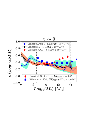
In this subsection we investigate the effect of Active Galactic Nuclei (AGN) feedback and Supernovae (SN) feedback on the - relation. To do so we compare 3 different configurations that have the same resolution and box size but have different subgrid physics recipes. These include:
-
•
L50N752-Ref, which is a simulation with the same feedback prescriptions and resolution as the EAGLE reference model L100N1504-Ref (dark solid line of Fig. 4),
-
•
L50N752-NoAGN, which has the same Physics and resolution as L50N752-Ref but does not include AGN feedback (dotted red line of Fig. 4),
-
•
L50N752-OnlyAGN, which has the same Physics, boxsize and resolution as L50N752-Ref but does not include SN feedback (blue dashed line of Fig. 4).
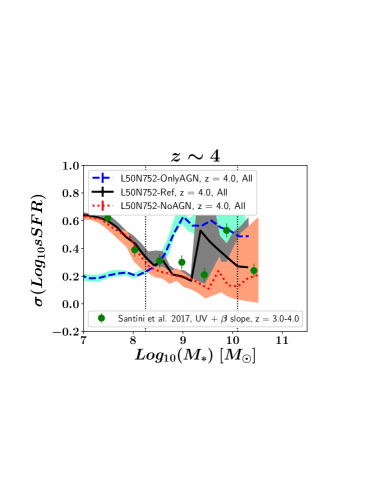
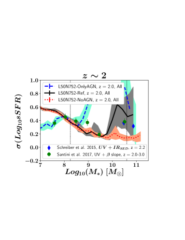
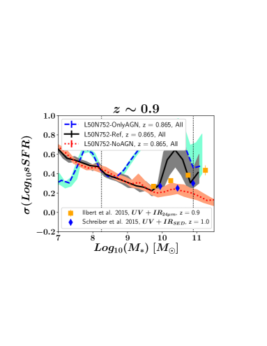
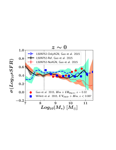
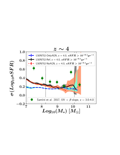
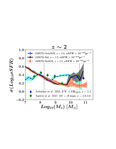
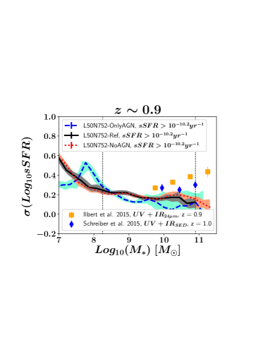
In Fig. 4 we present the effect of feedback prescriptions on the - relation in the EAGLE simulations. Guo et al. (2013) and Guo et al. (2015) find an increasing scatter with mass and suggest that halo/stellar-mass dependent processes such as disk instabilities, bar-driven tidal disruption, minor mergers and major mergers/interactions or stellar feedback are important for large objects. However, the comparison between the reference model (L50N752-Ref, black solid line) and the configuration which does not include the AGN feedback prescription (L50N752-NoAGN, red dotted line) suggests that the effect of the AGN feedback mechanism is mostly responsible for increasing the scatter of the relation for high mass objects ( ). The prescription increases the diversity in star formation histories at the regime (Figs 4 and 5) by creating a large number of quenched objects at the high mass end. We note that the absence of SN feedback would result in a more aggressive AGN feedback mechanism, which would significantly increase the dispersion for high mass galaxies (blue dashed line). This shows the interplay between the two different prescriptions and the finding is in agreement with the work of Bower et al. (2017), which suggests that black hole growth is suppressed by stellar feedback. If there are no galactic winds to decrease the accretion rate for a galaxy with a supermassive black hole, then the later will become bigger and its AGN feedback mechanism will affect more severely the sSFR of the object333In our AGN feedback scheme halos more massive than the threshold are seeded with a Supermassive Black Hole (SMBH), thus even relatively small galaxies at the range which reside halos with are affected, since the absence of the SNe feedback which would be important at this mass interval allows a fast and significant SMBH growth, which otherwise would not be possible.. The effect of the AGN feedback for the case of the L50N752-OnlyAGN run (in which SNe feedback is absent) is significant at z , an epoch when the SFRs of simulated objects would be influenced significantly from SNe feedback (For more details see Fig. 7 in Katsianis et al. (2017b) which describes the effect of SNe feedback on the star formation rate function). In contrast with - and - (Figs 4 and 5), we find that the - relation is not affected by feedback mechanisms (Fig. 6). The different fractions of quenched objects between configurations which employ different feedback prescriptions does not affect the comparison between them since the quenched objects, which increase the scatter, would in any simulation be excluded with the strict selection criterion adopted.
Santini et al. (2017) used the Hubble Space Telescope Frontier Fields to study the main sequence and its scatter. In contrast with Guo et al. (2013) and Ilbert et al. (2015) the authors found a decreasing scatter with mass at all redshifts they considered and they suggested that this behavior is a consequence of the smaller number of progenitors of low mass galaxies in a hierarchical scenario and/or of the efficient stellar feedback processes in low mass halos. Comparing the reference model (L50N752-Ref, black solid line) with the configuration which does not include the SN feedback mechanism (L50N752-OnlyAGN, blue dashed line) we see that the effect of this mechanism is indeed to increase the scatter of the relation with decreasing mass for low mass objects ( ). In addition, in low mass galaxies discrete gas accretion events trigger bursts of star formation which inject SNe feedback. Since feedback is very efficient in low mass galaxies this largely suppresses star formation until new gas is accreted (Faucher-Giguère, 2018, e.g.). However, the finding is below the resolution limit of 100 particles and higher resolution simulations are required to investigate this in the future (Figs 4 and 5).
In conclusion, AGN and SN feedback are playing a major role in producing the U-shape to the - and - relations described in subsection 3.1 and drive the evolution of the scatter. Both prescriptions give a range of SFHs both at the low- and high-mass ends with AGN feedback increasing the scatter mostly at the interval.
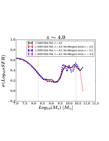
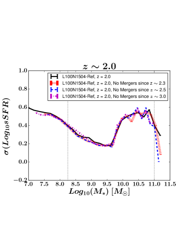
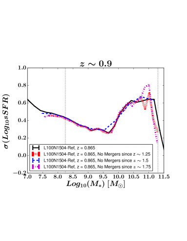
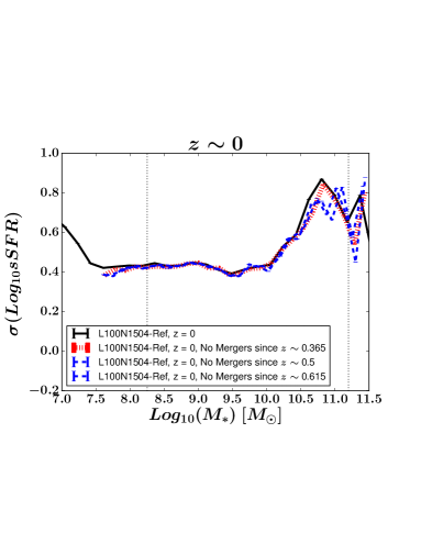
3.3 The effect of excluding mergers on the - relation.
Guo et al. (2015) pointed out that in massive galaxies interactions like minor and major mergers can induce starbursts followed by strong stellar feedback that can contribute significantly to the spread of sSFRs. In contrast, according to the authors, lower-mass galaxies are supposed to be less affected by the above and thus should have a smaller dispersion of SFHs leading to a scatter that increases with mass for the - relation. On the other hand, Peng et al. (2010) suggest that interacting/merging low-mass satellite galaxies are sensitive to environmental quenching and this could input a significant dispersion to the sSFRs at the low-mass end of the distribution. Orellana et al. (2017) reported that interactions between galaxies can affect the scatter for a range of masses. As Guo et al. (2015) suggest the effect of the above mechanisms to the sSFR dispersion are difficult to examine.
Qu et al. (2017) and Lagos et al. (2018b) studied the impact of mergers on mass assembly and angular momentum on the EAGLE galaxies. The authors found that the reference model is able to reproduce the observed merger rates and merger fractions of galaxies at various redshifts (Conselice et al., 2003; Kartaltepe et al., 2007; Ryan et al., 2008; Lotz et al., 2008; Conselice et al., 2009; de Ravel et al., 2009; Williams et al., 2011; López-Sanjuan et al., 2012; Bluck et al., 2012; Stott et al., 2013; Robotham et al., 2014; Man et al., 2016). Thus EAGLE can be used to study the effect of mergers on the - relation. We identify mergers using the merger trees available in the EAGLE database. These merger trees were created using the D-Trees algorithm of Jiang et al. (2014). Qu et al. (2017) described how this algorithm was adapted to work with EAGLE outputs. We consider that a merger (major or minor) occurs when the stellar mass ratio between the two merging systems, is above 0.1 (Crain et al., 2015). The separation criterion, , is defined as , where is the half-stellar mass radius of the primary galaxy (Qu et al., 2017). The above selection method to identify mergers and to separate into major or minor mergers is widely assumed in the EAGLE literature (Jiang et al., 2014; Crain et al., 2015; Qu et al., 2017; Lagos et al., 2018b). The fraction of mergers in the reference model at increases towards higher masses (Lagos et al., 2018b). Thus, it would be expected that the mechanism affects mostly the SFHs of high mass objects (Guo et al., 2015).
In Fig. 7 we present the effect of mergers on the - relation in the EAGLE simulations at . In the bottom panel the black line represents the reference model at , in which all galaxies are considered. The red dotted line represents the same but when ongoing mergers and objects that have experienced merging from are not included in the analysis. The blue dashed line describes the results when objects that have experienced merging from are excluded. The magenta represents the same when galaxies that have experienced merging from are excluded. The above analysis allows us to quantify the effect of ongoing (at ), ongoing + recent () and ongoing + recent + past () mergers to the - relation and has been done similarly for . We see that according to the reference model, mergers do not induce a significant dispersion in the star formation histories of galaxies. The above findings can be seen at all redshifts considered. This implies that recent mergers, despite their importance for galaxy formation and evolution, do not impart a significant scatter on the - relation.
4 The effect of SFR and stellar mass diagnostics on the - relation.
To obtain the intrinsic properties of galaxies, observers have to rely on models for the observed light. Stellar masses are typically calculated via the Spectral Energy Density (SED) fitting technique, while for the case of SFRs different authors employ different methods [e.g. Conversion of IR+UV luminosities to SFRs (Arnouts et al., 2013; Whitaker et al., 2014), SED fitting (Bruzual & Charlot, 2003), conversion of UV, H and IR luminosities (Katsianis et al., 2017b)]. However, there is an increasing number of reports that different techniques give different results, most likely due to systematic effects affecting the derived properties (Bauer et al., 2011; Utomo et al., 2014; Fumagalli et al., 2014; Katsianis et al., 2016; Davies et al., 2016, 2017). Boquien et al. (2014) argued that SFRs obtained from SED modeling, which take into account only FUV and U bands are overestimated. Hayward et al. (2014) noted that the SFRs obtained from IR luminosities (e.g. Noeske et al., 2007; Daddi et al., 2007a) can be artificially high. Ilbert et al. (2015) compared SFRs derived from SED and UV+IR, and find a tension reaching 0.25 dex. Guo et al. (2015) suggested that sSFR based on mid-IR emission may be significantly overestimated (Salim et al., 2009; Chang et al., 2015; Katsianis et al., 2017a, b). All the above uncertainties on the determination of intrinsic properties could possibly affect the observed/derived - relation.
Camps et al. (2016), Trayford et al. (2017) and Camps et al. (2018) presented a procedure to post-process the EAGLE galaxies and produce mock observations that describe how galaxies appear in various bands (e.g. GALEX-FUV, MIPS160, SPIRE500). The authors did so by performing a full 3D radiative transfer simulation to the EAGLE galaxies using the SKIRT code (Baes et al., 2003, 2011; Stalevski et al., 2012; Camps & Baes, 2015; Peest et al., 2017; Stalevski et al., 2016, 2017; Behrens et al., 2018). In this section we use the artificial SEDs present in Camps et al. (2018), in order to study how typical SFR/ diagnostics affect the - relation. We stress that the EAGLE objects that were post-processed by SKIRT were galaxies with stellar masses , above the resolution limit of 100 gas particles, and sufficient dust content. We use the Fitting and Assessment of Synthetic Templates (FAST) code (Kriek et al., 2009) to fit the mock SEDs to identify the SFRs and stellar masses of the EAGLE+SKIRT objects like in a range of observational studies (González et al., 2012, 2014; Botticella et al., 2017; Soto et al., 2017; Aird et al., 2018). Doing so enables us to evaluate the effect of different SFR/stellar mass diagnostics on the derived - relation and thus isolating the systematic effect on the . We assume an exponentially declining SFH []444We note that this parameterization despite the fact that is commonly used in the literature could misinterpret old stellar light for an exponentially increasing contribution originating from a younger stellar population. This can underestimate by a factor of two both SFRs and stellar masses. In addition, exponentially SFHs may not be representative in describing star forming galaxies (Ciesla et al., 2017; Iyer & Gawiser, 2017; Carnall et al., 2018; Leja et al., 2018). (Longhetti & Saracco, 2009; Michałowski et al., 2012; Botticella et al., 2012; Fumagalli et al., 2016; Blancato et al., 2017; Abdurro’uf & Akiyama, 2019), a Chabrier IMF (Chabrier, 2003), a Calzetti et al. (2000) dust attenuation law (Mitchell et al., 2013; Sklias et al., 2014; Cullen et al., 2018; McLure et al., 2018b) and a metallicity 0.02 (Ono et al., 2010; Greisel et al., 2013; Chan et al., 2016; McLure et al., 2018a). The above data are labelled in this work as L100N1504-Ref+SKIRT.
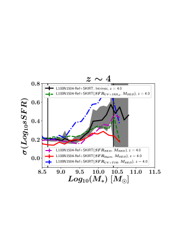
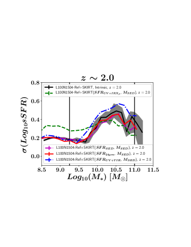
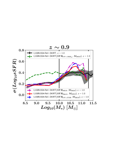
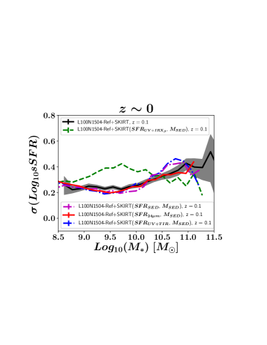
The black line of Fig. 8 represents the intrinsic scatter of the sSFRs of the EAGLE+SKIRT objects (intrinsic SFRs and stellar masses). The vertical lines define the mass interval at which the above data fully represent the total EAGLE sample. The shaded grey region represents the 95 % bootstrap confidence interval for 5000 re-samples for the - relation. For clarity we present the above only for the reference model. The main results are the following:
-
•
The magenta dashed line describes the - relation when SFRs and stellar masses are both inferred using the SED fitting technique from the mock survey. The method is used in a range of observational studies to obtain the relation and its scatter (de Barros et al., 2014; Salmon et al., 2015). According to the EAGLE+SKIRT data we see that the shape remain relatively unchanged with respect to the intrinsic relation (black solid line), but the scatter is slightly underestimated ( 0.5 dex) at the high mass end at but overestimated by dex at the mass interval of . The above gives the false impression that the scatter increases more sharply with mass.
-
•
The dark green dashed line represents the - relation when SFRs are obtained using the FUV luminosity (Kennicutt & Evans, 2012) and the IRX- relation (Meurer et al., 1999; Bouwens et al., 2012; Katsianis et al., 2017a) while the stellar masses are calculated through the SED fitting technique. This combination to obtain properties is widely used in the literature to estimate the relation and its scatter (Santini et al., 2017). We see that this method implies an artificially higher (with respect the intrinsic-black solid line) at the low mass end. This gives an artificial mass independent - relation with a scatter of dex, which is not evolving significantly from to .
-
•
The red solid line is the - relation retrieved when stellar masses are calculated via SED fitting and SFRs by combining the FUV and Infrared luminosity estimated from the luminosity (Kennicutt & Evans, 2012; Dale & Helou, 2002). Combining IR and UV luminosities to obtain SFRs in observations is a clasic method in the literature (Daddi et al., 2007b; Santini et al., 2009; Heinis et al., 2014) to obtain the relation. At the scatter is underestimated with respect the reference black line by dex at high masses and imply a dispersion with a constant scatter around 0.15 dex. At lower redshifts there is a good agreement (within 0.05 dex) from the reference intrinsic black line.
-
•
The blue dotted line describes the - relation when SFRs are derived from UVTIR and stellar masses from the SED fitting technique. According to the EAGLE+SKIRT data this technique agrees well with the intrinsic relation, except redshift 4 where the derived relation is mass independent with a scatter of 0.2 dex. Similarly with the magenta line, which represents the results from SED fitting) the scatter is overestimated with respect the reference black line by dex for high mass objects at the mass interval of for .
In conclusion, according to the EAGLE+SKIRT data, the inferred shape and normalization of the - relation can be affected by the methodology used to derive SFRs and stellar masses in observations. This can affect the conclusions about its shape and it is important for future observations to investigate this further (Davies et al., 2019). However, we note that having access to IR data and deriving SFRs and stellar masses from SED fitting or combined UV+IR luminosities typically give a - relation close to the intrinsic simulated relation and can probe successfully the shape of the relation for .
5 Conclusion and discussion
The - relation reflects the diversity of star formation histories for galaxies at different masses. However, it is difficult to decipher the true shape of the relation, the intrinsic value of the scatter and which mechanisms important for galaxy evolution govern it, solely by relying on observations. In this paper we presented the evolution of the intrinsic - relation employing the EAGLE suite of cosmological simulations and a compilation of multiwavelength observations at various redshifts. We deem the EAGLE suite appropriate for this study as it is able to reproduce the observed star formation rate and stellar mass functions (Furlong et al., 2015; Katsianis et al., 2017b) for a wide range of SFRs, stellar masses and redshifts. The investigation is not limited by the shortcomings encountered by galaxy surveys and address a range of redshifts and mass intervals. Our main conclusions are summarized as follows:
-
•
In agreement with recent observational studies (Guo et al., 2013; Ilbert et al., 2015; Willett et al., 2015; Santini et al., 2017) the EAGLE reference model suggests that the - relation is evolving with redshift and the dispersion is mass dependent (Section 3.1). This is in contrast with the widely accepted notion that the dispersion is mass/redshift independent with a constant scatter (Noeske et al., 2007; Elbaz et al., 2007; Rodighiero et al., 2010; Whitaker et al., 2012). We find that the - relation has a U-shape form with the scatter increasing both at the high and low mass ends. Any interpretations of an increasing (Guo et al., 2013; Ilbert et al., 2015) or decreasing dispersion (Santini et al., 2017) with mass may be misguided, since they usually focus on limited mass intervals (Subsection 3.2). The finding about the U-shape form of the relation is supported by results relying on the GAMA survey (Davies et al., 2019) at .
-
•
AGN and SN feedback are driving the shape and evolution of the - relation in the simulations (Subsection 3.2) . Both mechanisms cause a diversity of star formation histories for low mass (SN feedback) and high mass galaxies (AGN feedback).
-
•
Mergers do not play a major role on the shape of the - relation (Subsection 3.3).
-
•
We employ the EAGLE/SKIRT mock data to investigate how different diagnostics affect the - relation. The shape of the relation remains relatively unchanged if both the SFRs and stellar masses are inferred through SED fitting, or combined UV+IR data. However, SFRs that rely solely on UV data and the IRX- relation for dust corrections imply a constant scatter with stellar mass with almost no redshift evolution. Methodology used to derive SFRs and stellar masses can affect the inferred - relation in observations and thus compromising the robustness of conclusions about its shape and normalization.
Acknowledgments
We would like to thank the anonymous referee for their suggestions and comments which improved significantly our manuscript. In addition, we would like to thank Jorryt Matthee for discussions and suggestions. This work used the DiRAC Data Centric system at Durham University, operated by the Institute for Computational Cosmology on behalf of the STFC DiRAC HPC Facility (www.dirac.ac.uk). A.K has been supported by the Tsung-Dao Lee Institute Fellowship, Shanghai Jiao Tong University and CONICYT/FONDECYT fellowship, project number: 3160049. G.B. is supported by CONICYT/FONDECYT, Programa de Iniciacion, Folio 11150220. V.G. was supported by CONICYT/FONDECYT iniciation grant number 11160832. X.Z.Z. thanks supports from the National Key Research and Development Program of China (2017YFA0402703), NSFC grant (11773076) and the Chinese Academy of Sciences (CAS) through a grant to the CAS South America Center for Astronomy (CASSACA) in Santiago, Chile. AK would like to thank his family and especially George Katsianis, Aggeliki Spyropoulou John Katsianis and Nefeli Siouti for emotional support. He would also like to thank Sophia Savvidou for her IT assistance.
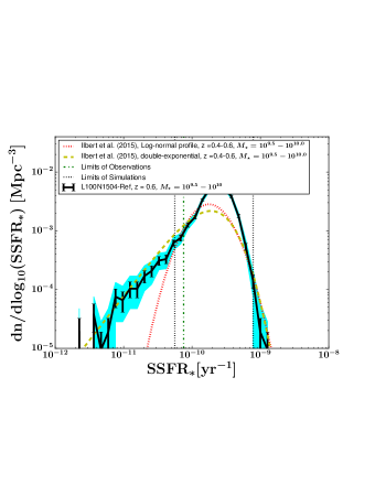
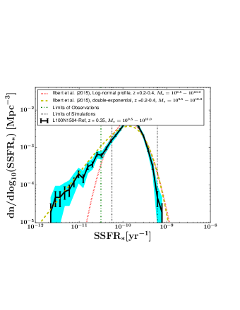
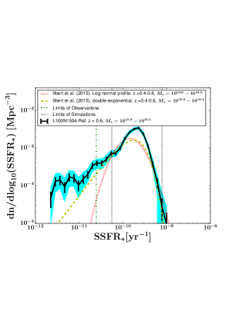
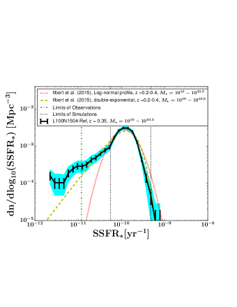
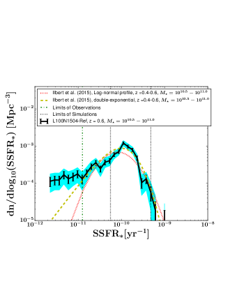
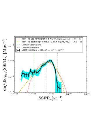
Appendix A The evolution of the specific star formation rate function.
In this appendix, we base our analysis of the dispersion of the sSFRs at different mass intervals on their distribution/histogram, namely the specific Star Formation Rate Function (sSFRF), following Ilbert et al. (2015), because studies of the dispersion that rely solely on 2d scatter plots (i.e. displays of the location of the individual sources in the plane) are not able to provide a quantitative information of how galaxies are distributed around the mean sSFR and cannot account for galaxies that could be under-sampled or missed by selection effects. In section 3.1 we present the evolution of the - relation at in order to visualize the scatter across galaxies, its shape and its evolution. We present the distribution of the sSFR of the EAGLE reference model (L100N1504-Ref) and compare it with observations (Ilbert et al., 2015) in Fig. 9 () and Fig. 10 (). The EAGLE SFRs are reported to be 0.2 dex lower than observations but are able to replicate the observed evolution and shape of the Cosmic Star Formation Rate Density (Furlong et al., 2015; Katsianis et al., 2017b), evolution of star formation rate function (Katsianis et al., 2017b) and SFR-BHAR (McAlpine et al., 2017). Following, McAlpine et al. (2017) we decrease the observed sSFRs by 1.58 in order to focus solely on the scatter of the distribution and its shape. We note that this discrepancy may have its roots to the methodologies used by observers to obtain the intrinsic SFRs and stellar masses (Katsianis et al., 2017a).
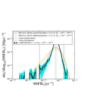
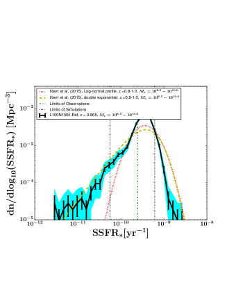
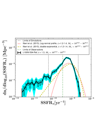
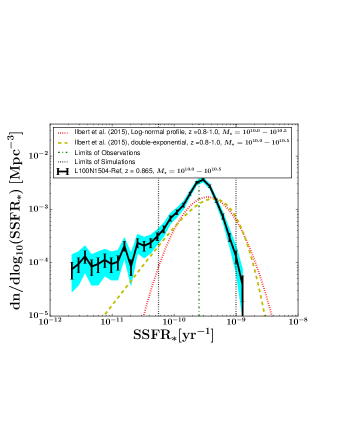
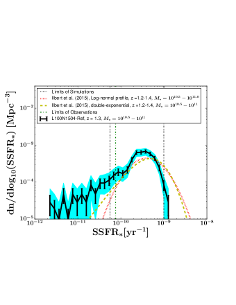

In the top panels of Fig. 9 and Fig. 10 we present the comparison between the simulated and observed data. The black solid line corresponds to the results from the EAGLE reference model, while the orange dashed line (double-exponentional) and red dotted lines (log-normal profile) represent the fits for the observed distribution. The green vertical line mark the limits of the observations. The cyan area represents the 95 bootstrap confidence interval for 1000 re-samples of the EAGLE SFRs, while the black errorbars represent the 1 sigma poissonian errors. We can see that the agreement between the simulated and observed sSFR functions is typically good at low mass objects but breaks down for galaxies more massive than , at with the L100N1504-Ref distribution being shifted to lower sSFR and having larger peak values in comparison with the observations. Ilbert et al. (2015) were not able to directly constrain the full shape of the sSFR function, despite the fact that they combined both GOODS and COSMOS data. In most of the redshift and mass bins, the sSFR function is incomplete below the peak in sSFR. The authors tried to discriminate between a log-normal and a double-exponential profile but were not able to sample sufficiently low sSFR to see any advantage of using either one or the other parametrization. They argued that the fit with a double-exponential function is more suitable than the log-normal function at . The EAGLE reference model points to the direction that the sSFRF at the different mass bins and redshifts follows a double-exponential function. However, for higher redshifts the simulated distributions are slightly flatter than the double-exponential fits of the observations. A double-exponential profile, that is not commonly used to describe the sSFR distribution (Ilbert et al., 2015), allows a significant density of star-forming galaxies with a low sSFR and the confirmation of this shape from future observations is important.
References
- Abbott et al. (2017) Abbott, T., Cooke, J., Curtin, C., et al. 2017, PASA, 34, e012
- Abdurro’uf & Akiyama (2019) Abdurro’uf, & Akiyama, M. 2019, arXiv e-prints, arXiv:1902.07712
- Aird et al. (2018) Aird, J., Coil, A. L., & Georgakakis, A. 2018, MNRAS, 474, 1225
- Anglés-Alcázar et al. (2017) Anglés-Alcázar, D., Faucher-Giguère, C.-A., Quataert, E., et al. 2017, MNRAS, 472, L109
- Arnouts et al. (2013) Arnouts, S., Le Floc’h, E., Chevallard, J., et al. 2013, A&A, 558, A67
- Baes et al. (2011) Baes, M., Verstappen, J., De Looze, I., et al. 2011, ApJS, 196, 22
- Baes et al. (2003) Baes, M., Davies, J. I., Dejonghe, H., et al. 2003, MNRAS, 343, 1081
- Baldry et al. (2012) Baldry, I. K., Driver, S. P., Loveday, J., et al. 2012, MNRAS, 421, 621
- Baldwin et al. (1981) Baldwin, J. A., Phillips, M. M., & Terlevich, R. 1981, PASP, 93, 5
- Bauer et al. (2011) Bauer, A. E., Conselice, C. J., Pérez-González, P. G., et al. 2011, MNRAS, 417, 289
- Bauer et al. (2013) Bauer, A. E., Hopkins, A. M., Gunawardhana, M., et al. 2013, MNRAS, 434, 209
- Behrens et al. (2018) Behrens, C., Pallottini, A., Ferrara, A., Gallerani, S., & Vallini, L. 2018, ArXiv e-prints, arXiv:1802.07772
- Blanc et al. (2019) Blanc, G. A., Lu, Y., Benson, A., Katsianis, A., & Barraza, M. 2019, arXiv e-prints, arXiv:1904.02721
- Blancato et al. (2017) Blancato, K., Genel, S., & Bryan, G. 2017, ApJ, 845, 136
- Bluck et al. (2012) Bluck, A. F. L., Conselice, C. J., Buitrago, F., et al. 2012, ApJ, 747, 34
- Boogaard et al. (2018) Boogaard, L. A., Brinchmann, J., Bouché, N., et al. 2018, A&A, 619, A27
- Boquien et al. (2014) Boquien, M., Buat, V., & Perret, V. 2014, A&A, 571, A72
- Botticella et al. (2012) Botticella, M. T., Smartt, S. J., Kennicutt, R. C., et al. 2012, A&A, 537, A132
- Botticella et al. (2017) Botticella, M. T., Cappellaro, E., Greggio, L., et al. 2017, A&A, 598, A50
- Bouwens et al. (2012) Bouwens, R. J., Illingworth, G. D., Oesch, P. A., et al. 2012, ApJ, 754, 83
- Bower et al. (2017) Bower, R. G., Schaye, J., Frenk, C. S., et al. 2017, MNRAS, 465, 32
- Bruzual & Charlot (2003) Bruzual, G., & Charlot, S. 2003, MNRAS, 344, 1000
- Cañas et al. (2018) Cañas, R., Elahi, P. J., Welker, C., et al. 2018, ArXiv e-prints, arXiv:1806.11417
- Calzetti et al. (2000) Calzetti, D., Armus, L., Bohlin, R. C., et al. 2000, ApJ, 533, 682
- Camps & Baes (2015) Camps, P., & Baes, M. 2015, Astronomy and Computing, 9, 20
- Camps et al. (2016) Camps, P., Trayford, J. W., Baes, M., et al. 2016, MNRAS, 462, 1057
- Camps et al. (2018) Camps, P., Trcka, A., Trayford, J., et al. 2018, ApJS, 234, 20
- Cano-Díaz et al. (2016) Cano-Díaz, M., Sánchez, S. F., Zibetti, S., et al. 2016, ApJ, 821, L26
- Carnall et al. (2018) Carnall, A. C., McLure, R. J., Dunlop, J. S., & Davé, R. 2018, MNRAS, 480, 4379
- Chabrier (2003) Chabrier, G. 2003, PASP, 115, 763
- Chan et al. (2016) Chan, J. C. C., Beifiori, A., Mendel, J. T., et al. 2016, MNRAS, 458, 3181
- Chang et al. (2015) Chang, Y.-Y., van der Wel, A., da Cunha, E., & Rix, H.-W. 2015, ApJS, 219, 8
- Chiosi et al. (2017) Chiosi, C., Sciarratta, M., Donofrio, M., et al. 2017, ApJ, 851, 44
- Ciesla et al. (2017) Ciesla, L., Elbaz, D., & Fensch, J. 2017, A&A, 608, A41
- Cluver et al. (2017) Cluver, M. E., Jarrett, T. H., Dale, D. A., et al. 2017, ApJ, 850, 68
- Conselice et al. (2003) Conselice, C. J., Chapman, S. C., & Windhorst, R. A. 2003, ApJ, 596, L5
- Conselice et al. (2009) Conselice, C. J., Yang, C., & Bluck, A. F. L. 2009, MNRAS, 394, 1956
- Crain et al. (2015) Crain, R. A., Schaye, J., Bower, R. G., et al. 2015, MNRAS, 450, 1937
- Crain et al. (2017) Crain, R. A., Bahé, Y. M., Lagos, C. d. P., et al. 2017, MNRAS, 464, 4204
- Cullen et al. (2018) Cullen, F., McLure, R. J., Khochfar, S., et al. 2018, MNRAS, 476, 3218
- Daddi et al. (2007a) Daddi, E., Dickinson, M., Morrison, G., et al. 2007a, ApJ, 670, 156
- Daddi et al. (2007b) Daddi, E., Alexander, D. M., Dickinson, M., et al. 2007b, ApJ, 670, 173
- Dale & Helou (2002) Dale, D. A., & Helou, G. 2002, ApJ, 576, 159
- Dalla Vecchia & Schaye (2012) Dalla Vecchia, C., & Schaye, J. 2012, MNRAS, 426, 140
- Davies et al. (2016) Davies, L. J. M., Driver, S. P., Robotham, A. S. G., et al. 2016, MNRAS, 461, 458
- Davies et al. (2017) Davies, L. J. M., Huynh, M. T., Hopkins, A. M., et al. 2017, MNRAS, 466, 2312
- Davies et al. (2019) Davies, L. J. M., Lagos, C. d. P., Katsianis, A., et al. 2019, MNRAS, 483, 1881
- Davis et al. (1985) Davis, M., Efstathiou, G., Frenk, C. S., & White, S. D. M. 1985, ApJ, 292, 371
- de Barros et al. (2014) de Barros, S., Schaerer, D., & Stark, D. P. 2014, A&A, 563, A81
- De Los Reyes et al. (2014) De Los Reyes, M., Lee, J. C., Ly, C., et al. 2014, in American Astronomical Society Meeting Abstracts, Vol. 223, American Astronomical Society Meeting Abstracts 223, 227.02
- de Ravel et al. (2009) de Ravel, L., Le Fèvre, O., Tresse, L., et al. 2009, A&A, 498, 379
- Dekel et al. (2009) Dekel, A., Birnboim, Y., Engel, G., et al. 2009, Nature, 457, 451
- Dolag & Stasyszyn (2009) Dolag, K., & Stasyszyn, F. 2009, MNRAS, 398, 1678
- Driver et al. (2011) Driver, S. P., Hill, D. T., Kelvin, L. S., et al. 2011, MNRAS, 413, 971
- Driver et al. (2016a) Driver, S. P., Wright, A. H., Andrews, S. K., et al. 2016a, MNRAS, 455, 3911
- Driver et al. (2016b) Driver, S. P., Andrews, S. K., Davies, L. J., et al. 2016b, ApJ, 827, 108
- Dutton et al. (2010) Dutton, A. A., van den Bosch, F. C., & Dekel, A. 2010, MNRAS, 405, 1690
- Eales et al. (2018) Eales, S., Smith, D., Bourne, N., et al. 2018, MNRAS, 473, 3507
- Elagali et al. (2018) Elagali, A., Lagos, C. D. P., Wong, O. I., et al. 2018, ArXiv e-prints, arXiv:1807.08251
- Elbaz et al. (2007) Elbaz, D., Daddi, E., Le Borgne, D., et al. 2007, A&A, 468, 33
- Faucher-Giguère (2018) Faucher-Giguère, C.-A. 2018, MNRAS, 473, 3717
- Fumagalli et al. (2014) Fumagalli, M., Labbé, I., Patel, S. G., et al. 2014, ApJ, 796, 35
- Fumagalli et al. (2016) Fumagalli, M., Franx, M., van Dokkum, P., et al. 2016, ApJ, 822, 1
- Furlong et al. (2015) Furlong, M., Bower, R. G., Theuns, T., et al. 2015, MNRAS, 450, 4486
- Furlong et al. (2017) Furlong, M., Bower, R. G., Crain, R. A., et al. 2017, MNRAS, 465, 722
- García et al. (2017) García, L. A., Tescari, E., Ryan-Weber, E. V., & Wyithe, J. S. B. 2017, MNRAS, 470, 2494
- González et al. (2014) González, V., Bouwens, R., Illingworth, G., et al. 2014, ApJ, 781, 34
- González et al. (2012) González, V., Bouwens, R. J., Labbé, I., et al. 2012, ApJ, 755, 148
- Greisel et al. (2013) Greisel, N., Seitz, S., Drory, N., et al. 2013, ApJ, 768, 117
- Guo et al. (2013) Guo, K., Zheng, X. Z., & Fu, H. 2013, ApJ, 778, 23
- Guo et al. (2015) Guo, K., Zheng, X. Z., Wang, T., & Fu, H. 2015, ApJ, 808, L49
- Hayward et al. (2014) Hayward, C. C., Lanz, L., Ashby, M. L. N., et al. 2014, MNRAS, 445, 1598
- Heinis et al. (2014) Heinis, S., Buat, V., Béthermin, M., Bock, J., et al. 2014, MNRAS, 437, 1268
- Hopkins et al. (2014) Hopkins, P. F., Kereš, D., Oñorbe, J., et al. 2014, MNRAS, 445, 581
- Ilbert et al. (2015) Ilbert, O., Arnouts, S., Le Floc’h, E., et al. 2015, A&A, 579, A2
- Iyer & Gawiser (2017) Iyer, K., & Gawiser, E. 2017, ApJ, 838, 127
- Jiang et al. (2014) Jiang, L., Helly, J. C., Cole, S., & Frenk, C. S. 2014, MNRAS, 440, 2115
- Kajisawa et al. (2010) Kajisawa, M., Ichikawa, T., Yamada, T., et al. 2010, ApJ, 723, 129
- Kartaltepe et al. (2007) Kartaltepe, J. S., Sanders, D. B., Scoville, N. Z., et al. 2007, ApJS, 172, 320
- Katsianis et al. (2017a) Katsianis, A., Tescari, E., Blanc, G., & Sargent, M. 2017a, MNRAS, 464, 4977
- Katsianis et al. (2015) Katsianis, A., Tescari, E., & Wyithe, J. S. B. 2015, MNRAS, 448, 3001
- Katsianis et al. (2016) —. 2016, PASA, 33, e029
- Katsianis et al. (2017b) Katsianis, A., Blanc, G., Lagos, C. P., et al. 2017b, MNRAS, 472, 919
- Kelson (2014) Kelson, D. D. 2014, arXiv e-prints, arXiv:1406.5191
- Kennicutt & Evans (2012) Kennicutt, R. C., & Evans, N. J. 2012, ARA&A, 50, 531
- Kriek et al. (2009) Kriek, M., van Dokkum, P. G., Labbé, I., et al. 2009, ApJ, 700, 221
- Kurczynski et al. (2016) Kurczynski, P., Gawiser, E., Acquaviva, V., et al. 2016, ApJ, 820, L1
- Lagos et al. (2017) Lagos, C. d. P., Theuns, T., Stevens, A. R. H., et al. 2017, MNRAS, 464, 3850
- Lagos et al. (2018a) Lagos, C. d. P., Tobar, R. J., Robotham, A. S. G., et al. 2018a, MNRAS, 481, 3573
- Lagos et al. (2015) Lagos, C. d. P., Crain, R. A., Schaye, J., et al. 2015, MNRAS, 452, 3815
- Lagos et al. (2018b) Lagos, C. d. P., Stevens, A. R. H., Bower, R. G., et al. 2018b, MNRAS, 473, 4956
- Leja et al. (2018) Leja, J., Johnson, B. D., Conroy, C., & van Dokkum, P. 2018, ApJ, 854, 62
- Li & White (2009) Li, C., & White, S. D. M. 2009, MNRAS, 398, 2177
- Longhetti & Saracco (2009) Longhetti, M., & Saracco, P. 2009, MNRAS, 394, 774
- López-Sanjuan et al. (2012) López-Sanjuan, C., Le Fèvre, O., Ilbert, O., et al. 2012, A&A, 548, A7
- Lotz et al. (2008) Lotz, J. M., Davis, M., Faber, S. M., et al. 2008, ApJ, 672, 177
- Man et al. (2016) Man, A. W. S., Zirm, A. W., & Toft, S. 2016, ApJ, 830, 89
- Matthee & Schaye (2018) Matthee, J., & Schaye, J. 2018, ArXiv e-prints, arXiv:1805.05956
- McAlpine et al. (2017) McAlpine, S., Bower, R. G., Harrison, C. M., et al. 2017, MNRAS, 468, 3395
- McConnell & Ma (2013) McConnell, N. J., & Ma, C.-P. 2013, ApJ, 764, 184
- McLure et al. (2018a) McLure, R. J., Dunlop, J. S., Cullen, F., et al. 2018a, MNRAS, 476, 3991
- McLure et al. (2018b) McLure, R. J., Pentericci, L., Cimatti, A., et al. 2018b, MNRAS, 479, 25
- Meurer et al. (1999) Meurer, G. R., Heckman, T. M., & Calzetti, D. 1999, ApJ, 521, 64
- Michałowski et al. (2012) Michałowski, M. J., Dunlop, J. S., Cirasuolo, M., et al. 2012, A&A, 541, A85
- Mitchell et al. (2013) Mitchell, P. D., Lacey, C. G., Baugh, C. M., & Cole, S. 2013, MNRAS, 435, 87
- Noeske et al. (2007) Noeske, K. G., Weiner, B. J., Faber, S. M., et al. 2007, ApJ, 660, L43
- Ono et al. (2010) Ono, Y., Ouchi, M., Shimasaku, K., et al. 2010, MNRAS, 402, 1580
- Orellana et al. (2017) Orellana, G., Nagar, N. M., Elbaz, D., et al. 2017, A&A, 602, A68
- Peest et al. (2017) Peest, C., Camps, P., Stalevski, M., Baes, M., & Siebenmorgen, R. 2017, A&A, 601, A92
- Peng et al. (2010) Peng, Y.-j., Lilly, S. J., Kovač, K., et al. 2010, ApJ, 721, 193
- Pillepich et al. (2018) Pillepich, A., Springel, V., Nelson, D., et al. 2018, MNRAS, 473, 4077
- Qin et al. (2018) Qin, Y., Duffy, A. R., Mutch, S. J., et al. 2018, MNRAS, arXiv:1802.03879
- Qu et al. (2017) Qu, Y., Helly, J. C., Bower, R. G., et al. 2017, MNRAS, 464, 1659
- Renzini & Peng (2015) Renzini, A., & Peng, Y.-j. 2015, ApJ, 801, L29
- Robotham et al. (2014) Robotham, A. S. G., Driver, S. P., Davies, L. J. M., et al. 2014, MNRAS, 444, 3986
- Rodighiero et al. (2010) Rodighiero, G., Cimatti, A., Gruppioni, C., Popesso, P., et al. 2010, A&A, 518, L25
- Rosas-Guevara et al. (2016) Rosas-Guevara, Y., Bower, R. G., Schaye, J., et al. 2016, MNRAS, 462, 190
- Ryan et al. (2008) Ryan, Jr., R. E., Cohen, S. H., Windhorst, R. A., & Silk, J. 2008, ApJ, 678, 751
- Salim et al. (2007) Salim, S., Rich, R. M., Charlot, S., Brinchmann, J., et al. 2007, ApJS, 173, 267
- Salim et al. (2009) Salim, S., Dickinson, M., Michael Rich, R., et al. 2009, ApJ, 700, 161
- Salmon et al. (2015) Salmon, B., Papovich, C., Finkelstein, S. L., et al. 2015, ApJ, 799, 183
- Sánchez et al. (2018) Sánchez, S. F., Avila-Reese, V., Hernandez-Toledo, H., et al. 2018, Rev. Mexicana Astron. Astrofis., 54, 217
- Santini et al. (2009) Santini, P., Fontana, A., Grazian, A., et al. 2009, A&A, 504, 751
- Santini et al. (2017) Santini, P., Fontana, A., Castellano, M., et al. 2017, ApJ, 847, 76
- Schaller et al. (2015) Schaller, M., Dalla Vecchia, C., Schaye, J., et al. 2015, MNRAS, 454, 2277
- Schaye (2004) Schaye, J. 2004, ApJ, 609, 667
- Schaye & Dalla Vecchia (2008) Schaye, J., & Dalla Vecchia, C. 2008, MNRAS, 383, 1210
- Schaye et al. (2015) Schaye, J., Crain, R. A., Bower, R. G., et al. 2015, MNRAS, 446, 521
- Schreiber et al. (2015) Schreiber, C., Pannella, M., Elbaz, D., et al. 2015, A&A, 575, A74
- Sklias et al. (2014) Sklias, P., Zamojski, M., Schaerer, D., et al. 2014, A&A, 561, A149
- Soto et al. (2017) Soto, E., de Mello, D. F., Rafelski, M., et al. 2017, ApJ, 837, 6
- Sparre et al. (2015) Sparre, M., Hayward, C. C., Springel, V., et al. 2015, MNRAS, 447, 3548
- Springel (2005) Springel, V. 2005, MNRAS, 364, 1105
- Springel et al. (2001) Springel, V., Yoshida, N., & White, S. D. M. 2001, NA, 6, 79
- Stalevski et al. (2017) Stalevski, M., Asmus, D., & Tristram, K. R. W. 2017, MNRAS, 472, 3854
- Stalevski et al. (2012) Stalevski, M., Jovanović, P., Popović, L. Č., & Baes, M. 2012, MNRAS, 425, 1576
- Stalevski et al. (2016) Stalevski, M., Ricci, C., Ueda, Y., et al. 2016, MNRAS, 458, 2288
- Stott et al. (2013) Stott, J. P., Sobral, D., Smail, I., et al. 2013, MNRAS, 430, 1158
- Tescari et al. (2014) Tescari, E., Katsianis, A., Wyithe, J. S. B., et al. 2014, MNRAS, 438, 3490
- Tescari et al. (2018) Tescari, E., Cortese, L., Power, C., et al. 2018, MNRAS, 473, 380
- Torrey et al. (2017) Torrey, P., Hopkins, P. F., Faucher-Giguère, C.-A., et al. 2017, MNRAS, 467, 2301
- Trayford et al. (2015) Trayford, J. W., Theuns, T., Bower, R. G., et al. 2015, MNRAS, 452, 2879
- Trayford et al. (2017) Trayford, J. W., Camps, P., Theuns, T., et al. 2017, MNRAS, 470, 771
- Utomo et al. (2014) Utomo, D., Kriek, M., Labbé, I., Conroy, C., & Fumagalli, M. 2014, ApJ, 783, L30
- Wang et al. (2017) Wang, L., Chen, D.-M., & Li, R. 2017, MNRAS, 471, 523
- Weinberger et al. (2017) Weinberger, R., Springel, V., Hernquist, L., et al. 2017, MNRAS, 465, 3291
- Whitaker et al. (2012) Whitaker, K. E., van Dokkum, P. G., Brammer, G., & Franx, M. 2012, ApJ, 754, L29
- Whitaker et al. (2014) Whitaker, K. E., Franx, M., Leja, J., et al. 2014, ApJ, 795, 104
- Willett et al. (2015) Willett, K. W., Schawinski, K., Simmons, B. D., et al. 2015, MNRAS, 449, 820
- Williams et al. (2011) Williams, R. J., Quadri, R. F., & Franx, M. 2011, ApJ, 738, L25