Non-local control in the conduction coefficients:
well posedness and convergence to the local limit

Abstract:

We consider a problem of optimal distribution of conductivities in a system governed by a non-local diffusion law. The problem stems from applications in optimal design and more specifically topology optimization. We propose a novel parametrization of non-local material properties. With this parametrization the non-local diffusion law in the limit of vanishing non-local interaction horizons converges to the famous and ubiquitously used generalized Laplacian with SIMP (Solid Isotropic Material with Penalization) material model. The optimal control problem for the limiting local model is typically ill-posed and does not attain its infimum without additional regularization. Surprisingly, its non-local counterpart attains its global minima in many practical situations, as we demonstrate in this work. In spite of this qualitatively different behaviour, we are able to partially characterize the relationship between the non-local and the local optimal control problems. We also complement our theoretical findings with numerical examples, which illustrate the viability of our approach to optimal design practitioners.

Keywords:

Nonlocal optimal design, nonlocal optimal control in the coefficients, convergence to local problems, numerical approximation of nonlocal problems.

1 Introduction

Nonlocal problems receive a lot of attention nowadays owing to a wide range of applications they have in a variety of contexts. In particular, we mention micromechanics [Rog91], image processing [GO08], phase transitions [AB98], pattern formation [Fif03], population dispersal [CCEM07], optimal design [AM15a] and shape optimization [FBRS18], optimal control [DG14] and inverse problems [DG16]; see also a very recent monograph on the subject [Du19]. Among nonlocal problems, fractional or nonlocal diffusion plays a central role. It has attracted enormous interest and a great deal of work has been done over the past twenty years. The number of references on the subject and connections of nonlocal diffusion with remarkable applications is really overwhelming. We refer the interested readers to the monographs [AVMRTM10, BV16] and the references therein. In the context of continuum mechanics the non-local modelling goes back at least to the Eringen’s model [Eri02, EB18], and more recently has been focused on peridynamical modelling [Kun75, Sil00, MO17, Voy14, EW07, MD15]. These latter models refrain from using the gradients of the state fields with the goal of unified description of singular phenomena, such as fracture or dislocation. When considering scalar equations, such as for example the steady state heat equation, peridynamics equations may essentially be seen as a nonlocal diffusion equations on bounded domains [AM10, AM15b].

In this paper we consider a prototypical optimal design problem for diffusion phenomena, in which one has to determine the best way of distributing conducting materials inside a given computational domain. For models governed by the local diffusion phenomena such problems have been studied for a long time and are quite well understood, see for example [All12, BS03, Ped16] and references therein. As a very rough summary we can say that these problems are typically ill-posed and do not attain their infimum. One possible way of dealing with this issue is to bring the limits of minimizing sequences into consideration and interpret them as composite materials obtained from mixing the original materials in the sense described by the theory of homogenization. Another option is to restrict the set of considered material distributions by introducing constraints or penalty functions with regularizing effect. An extremely successful example of the latter approach, which is nowadays widely utilized in engineering practice, is the SIMP (Solid Isotropic Material with Penalization) material parametrization model combined with additional regularization techniques [BS03, BK88, Bou01, Sig97]. An interesting recent study, which can be interpreted in the light of comparing the two outlined approaches in the context of the steady state heat conduction, is [YSS18].

Research in optimal design of systems described by the non-local governing equations is in its infancy. Our present model is inspired by the recent studies [AM15a, AM17], where a very similar optimal design problem for a nonlocal diffusion state law was analyzed. The main novelty of our work is the way in which the material properties (conductivities) enter into the model. We chose a nonlocal interpolation of material properties that allows us to establish a natural link between the nonlocal optimal design problem and a local one in which material properties are interpolated by the SIMP scheme. Our main objective is to analyze this nonlocal optimal design problem and to characterize its relationship with the local optimal design problem as the nonlocal parameter (the interaction horizon) goes to zero. We have documented our preliminary findings in a brief note [EB19], where we have been primarily concerned with the qualitative relation between our non-local model and a particular heuristic regularization method (‘‘sensitivity filtering’’, see [Sig97]) for the local model with SIMP. This work includes the technical results, proofs, and numerical experiments, which have been omitted from [EB19] owing to the space requirements.

The outline of the paper is as follows. In Section 2 we formulate the non-local state equations and discuss their well-posedness. We also state the nonlocal optimal design problem, which is going to be the main subject of our study, as well as its local counterpart. Section 2 also includes Theorem 3, an interesting result illustrating the continuity of the conductivity-to-state map for the non-local problem. In Section 3 we include several existence results for the nonlocal optimal design problem depending on the SIMP penalization parameter. In Section 4 we address the convergence of the nonlocal problems to the local one and the connection of our proposed model with SIMP in the local case. Finally, in Section 5, a numerical approach to the nonlocal optimal design problems is described and several numerical examples are presented.

2 Problem formulation and perliminaries

2.1 Local control in the conduction coefficients

We begin our discussion with a well understood optimal control problem in the conduction coefficients of generalized Laplace equation, or topology optimization through material distribution, see for example [CM70, All12, BS03] and references therein. This problem will serve us both as a reference physical model and also as a limiting problem later on.

Let $\Omega\subset\mathbb{R}^{n}$, $n\geq 2$, be an open, bounded, and connected domain. In this domain we consider the generalized Laplace equation with a volumetric source $f\in L^{2}(\Omega)$, homogeneous Dirichlet boundary conditions, and a spatially heterogeneous diffusion (conduction) coefficient $\kappa^{\text{loc}}$. Its weak solution $u\in\mathcal{U}_{0}=W^{1,2}_{0}(\Omega)$ satisfies the variational statement

$$a_{\kappa^{\text{loc}}}(u,v)=\ell(v),\qquad\forall\>v\in\mathcal{U}_{0},$$ (1)

where the parametric bilinear form $a_{\kappa^{\text{loc}}}$ and the linear functional $\ell$ are given by

$$a_{\kappa^{\text{loc}}}(u,v) =\int_{\Omega}\kappa^{\text{loc}}(x)\nabla u(x)\cdot\nabla v(x)\,\mathrm{d}x,\quad\text{and}$$ (2)

$$\ell(v) =\int_{\Omega}f(x)v(x)\,\mathrm{d}x.$$

We recall that

$$u\text{\ solves\leavevmode\nobreak\ \eqref{eq:w_loc}}\quad\iff\quad u=\operatorname*{arg\,min}_{v\in\mathcal{U}_{0}}I_{\kappa^{\text{loc}}}(v):=\bigg{[}\frac{1}{2}a_{\kappa^{\text{loc}}}(v,v)-\ell(v)\bigg{]},$$ (3)

where $I_{\kappa^{\text{loc}}}$ is an associated quadratic energy functional. We will utilize the shorthand notation $\mathcal{S}^{\text{loc}}(\kappa^{\text{loc}}):=\operatorname*{arg\,min}_{v\in\mathcal{U}_{0}}I_{\kappa^{\text{loc}}}(v)$ for the control coefficient-to-state operator for this system.

In connection with this governing equation we consider a problem of optimal distribution of conductive material in $\Omega$ under simple constraints. Specifically, we will define the following convex set of admissible material distributions:

$$\mathcal{A}=\bigg{\{}\,\rho\in L^{\infty}(\Omega)\mid\underline{\rho}\leq\rho(\cdot)\leq\overline{\rho},\text{a.e.\ in $\Omega$},\int_{\Omega}\rho(x)\,\mathrm{d}x\leq\gamma|\Omega|\,\bigg{\}},$$ (4)

where $\gamma\in]\underline{\rho},\overline{\rho}[$ is a given volume fraction, and $0<\underline{\rho}<\underline{\rho}<\infty$ are given bounds. We assume that the local material conductivity $\kappa^{\text{loc}}$ is related to the control parameter $\rho\in\mathcal{A}^{\delta}$ through the so-called SIMP (Simple Interpolated Material with Penalization) model, see [BS03, All12]: $\kappa^{\text{loc}}(x)=\rho^{p}(x)$, where $p\geq 1$ plays a role of a penalty parameter in certain optimal design problems. Each $\rho\in\mathcal{A}^{\delta}$ is therefore mapped into $\kappa^{\text{loc}}$ satisfying the bounds $\underline{\kappa}=\underline{\rho}^{p}\leq\kappa^{\text{loc}}\leq\overline{\kappa}=\overline{\rho}^{p}$.

For a given performance functional $J:\mathcal{A}\times\mathcal{U}_{0}\to\mathbb{R}$ we consider the following optimization problem:

$$\operatorname*{minimize}_{\rho\in\mathcal{A}}J(\rho,\mathcal{S}^{\text{loc}}(\rho^{p})).$$ (5)

Note that the use of ‘‘$\operatorname*{minimize}$’’ instead of ‘‘$\inf$’’ does not automatically mean that the infimum is attained in (5). In fact, in most interesting situations this is not the case without additional regularization of the problem (5). We will return to this issue in Section 3.

Of particular interest to us will be the case of $J(\rho,u)=\ell(u)$, corresponding to compliance minimization. Note that in this case the reduced compliance can be expressed in a variety of ways:

$$\mathfrak{c}(\rho):=\ell(\mathcal{S}^{\text{loc}}(\rho^{p}))=a_{\rho^{p}}(\mathcal{S}^{\text{loc}}(\rho^{p}),\mathcal{S}^{\text{loc}}(\rho^{p}))=-2I_{\rho^{p}}(\mathcal{S}^{\text{loc}}(\rho^{p})).$$ (6)

The last expression in conjunction with (3) allows us to state the compliance minimization problem as a saddle point problem, which will be used later on.

2.2 Non-local state equation

We will now introduce a non-local analogue of the local governing equations (1), (2). We will use $\delta>0$ to denote the non-local interaction horizon, and $B(x,\delta)=\{\,y\in\mathbb{R}^{n}:|x-y|<\delta\,\}$ to denote an open ball of radius $\delta$ centered at $x\in\mathbb{R}^{n}$. Let $\Omega_{\delta}=\cup_{x\in\Omega}B(x,\delta)$ be the set of points located within distance $\delta$ from points in $\Omega$, and $\Gamma^{\text{nl}}=\Omega_{\delta}\setminus\Omega$ be the ‘‘non-local boundary’’ of $\Omega$. We consider nonlocal linear diffusion equations, that in this scalar framework can also be seen as peridynamics equations. Similarly to (1), they will be formulated with the help of the following parametric bilinear form $a_{\delta,\kappa}(\cdot,\cdot)$:

$$a_{\delta,\kappa}(u,v) =\int_{\Omega_{\delta}}\int_{\Omega_{\delta}}\kappa(x,x^{\prime})A_{\delta}(|x-x^{\prime}|)\frac{u(x)-u(x^{\prime})}{|x-x^{\prime}|}\frac{v(x)-v(x^{\prime})}{|x-x^{\prime}|}\,\mathrm{d}x\,\mathrm{d}x^{\prime},$$ (7)

while we use the same linear functional $\ell(\cdot)$ defined in (2). In the equations above, $\kappa\in L^{\infty}(\Omega_{\delta}\times\Omega_{\delta})$ is a ‘‘nonlocal conductivity’’, and $A_{\delta}:\mathbb{R}_{+}\to\mathbb{R}_{+}$ is a radial kernel satisfying certain conditions. More precisely, we assume that

$$\kappa\in\mathcal{K}^{\delta}=\{\,\tilde{\kappa}\in L^{\infty}(\Omega_{\delta}\times\Omega_{\delta})\mid\underline{\kappa}\leq\tilde{\kappa}(x,x^{\prime})=\tilde{\kappa}(x^{\prime},x)\leq\overline{\kappa},\forall x,x^{\prime}\in\Omega_{\delta}\,\},$$ (8)

for some $0<\underline{\kappa}<\overline{\kappa}<+\infty$, and that $A_{\delta}$ satisfies the following conditions:

$$\frac{1}{n}\int_{\mathbb{R}^{n}}A_{\delta}(|x|)\,\mathrm{d}x=1,$$ (9)

$$\operatorname{supp}A_{\delta}(|\cdot|)\subset B(0,\delta),\quad\forall\;\delta>0,$$ (10)

and there exists $s\in(0,1)$ and $c_{\delta}>0$ such that

$$A_{\delta}(|x|)\geq\frac{c_{\delta}}{|x|^{n+2s-2}},\quad\forall\;x\in B(0,\delta/2)\setminus\{0\},\delta>0.$$ (11)

Let $\mathcal{U}^{\delta}=\{\,u\in L^{2}(\Omega_{\delta})\mid a_{\delta,1}(u,u)<+\infty\,\}$, and $\mathcal{U}_{0}^{\delta}$ be the topological closure of $C^{\infty}_{c}(\Omega)$ (where we extend the functions in $C^{\infty}_{c}(\Omega)$ by $0$ outside of $\Omega$) in $\mathcal{U}_{\delta}$ with respect to the semi-inner product $a_{\delta,1}(\cdot,\cdot)$. Since the nonlocal conductivities are uniformly bounded from above and away from zero, for any $\kappa\in\mathcal{K}^{\delta}$ and $u\in\mathcal{U}^{\delta}$ we have the estimates

$$\underline{\kappa}a_{\delta,1}(u,u)\leq a_{\delta,\kappa}(u,u)\leq\overline{\kappa}a_{\delta,1}(u,u).$$

Consequently, $u\in{\mathcal{U}}^{\delta}$ if and only if $\|u\|_{L^{2}(\Omega_{\delta})}<+\infty$ and $a_{\delta,\kappa}(u,u)<+\infty$. In this notation, the non-local governing equations we will study can be stated as follows: find $u\in\mathcal{U}_{0}^{\delta}$ such that

$$a_{\delta,\kappa}(u,v)=\ell(v),\quad\forall v\in\mathcal{U}_{0}^{\delta}.$$ (12)

2.3 Non-local control in the conduction coefficients

We will now introduce a non-local analogue of (5), where the local governing equations (1), (2) are replaced with their non-local analogue introduced in the previous section. Similarly to (4), we define the following convex set of admissible material distributions:

$$\mathcal{A}^{\delta}=\bigg{\{}\,\rho\in L^{\infty}(\Omega_{\delta})\mid\underline{\rho}\leq\rho(\cdot)\leq\overline{\rho},\text{a.e.\ in $\Omega_{\delta}$},\int_{\Omega}\rho(x)\,\mathrm{d}x\leq\gamma|\Omega|\,\bigg{\}},$$ (13)

where the parameters are exactly as in (4). We still assume that the local material conductivity $\kappa^{\text{loc}}$ satisfies the SIMP model $\kappa^{\text{loc}}(x)=\rho^{p}(x)$, $x\in\Omega_{\delta}$. In addition, we assume that the non-local conductivity $\kappa(x,x^{\prime})$ entering (12) is simply a geometric mean of $\kappa^{\text{loc}}(x)$ and $\kappa^{\text{loc}}(x^{\prime})$, that is, $\kappa(x,x^{\prime})=\sqrt{\kappa^{\text{loc}}(x)\kappa^{\text{loc}}(x^{\prime})}=\rho^{p/2}(x)\rho^{p/2}(x^{\prime})$. For a given performance functional $J:\mathcal{A}^{\delta}\times\mathcal{U}^{\delta}\to\mathbb{R}$ we consider the following optimization problem:

$$\operatorname*{minimize}_{(\rho,u)\in\mathcal{A}^{\delta}\times\mathcal{U}_{0}^{\delta}}J(\rho,u),$$ (14)

$$\text{subject to $u$ solving\leavevmode\nobreak\ \eqref{eq:w} with $\kappa(x,x^{\prime})=\rho^{p/2}(x)\rho^{p/2}(x^{\prime})$}.$$

We will still refer to the case $J(\rho,u)=\ell(u)$ as the compliance minimization problem.

Remark 1.

Essentially, the only difference between the non-local optimal design problem considered here and the one in [AM15a] is the way the control variables enter the bilinear form. In order to preserve the symmetry of the form with respect to $(x,x^{\prime})$ one takes an average between the local conductivities at $x$ and $x^{\prime}$ to be the non-local conductivity in the bilinear form defining the non-local governing equations. The authors of [AM15a] take an arithmetic mean, whereas we use a geometric mean (for $p=1$) for the same purpose. Advantages of this choice will become clear when we discuss the relationship between the nonlocal problem described in this section and the incredibly popular and successful SIMP method for (local) optimal design outlined in Section 2.1.

2.4 Well-posedness and continuity of the conductivity-to-state operator

In this subsection we recall a couple of known results about the non-local equation (12).

Under the assumptions (9)–(11), $a_{\delta,1}(\cdot,\cdot)$ defines an inner product on $\mathcal{U}_{0}^{\delta}$ thereby making it a Hilbert space [AM15b]. We denote by $\|\cdot\|_{\mathcal{U}_{0}^{\delta}}$ the norm induced by this inner product. Furthermore, owing to (11), there are constants $\tilde{c}_{\delta}>0$, $\hat{c}_{\delta}>0$ independent from $u$ such that for any $\delta>0$, $\kappa\in\mathcal{K}^{\delta}$ and $u\in\mathcal{U}_{0}^{\delta}$ we have the inequalities

$$a_{\delta,\kappa}(u,u) \geq c_{\delta_{0}}\underline{\kappa}\int_{\Omega_{\delta}}\int_{\Omega_{\delta}\cap B(x,\delta/2)}\frac{(u(x)-u(x^{\prime}))^{2}}{|x-x^{\prime}|^{n+2s}}\,\mathrm{d}x^{\prime}\,\mathrm{d}x\geq\tilde{c}_{\delta}\underline{\kappa}\int_{\Omega_{\delta}}\int_{\Omega_{\delta}}\frac{(u(x)-u(x^{\prime}))^{2}}{|x-x^{\prime}|^{n+2s}}\,\mathrm{d}x^{\prime}\,\mathrm{d}x$$ (15)

$$\geq\hat{c}_{\delta}\underline{\kappa}\|u\|^{2}_{L^{2}(\Omega)},$$

where the second inequality is a consequence of [BMC14, Proposition 6.1] and the third inequality is established in [BMC14, Lemma 6.2]. When combined with Cauchy–Bunyakovsky–Schwarz inequality, (15) implies that $\ell:\mathcal{U}_{0}^{\delta}\to\mathbb{R}$ is a continuous linear functional with respect to $\|\cdot\|_{{\mathcal{U}}_{0}^{\delta}}$. Consequently we have verified the necessary assumptions for the application of Lax–Milgram Lemma (see, for example, [Bre10]) allowing us to conclude the following.

Theorem 2.

For each $\delta\in]0,\delta_{0}[$, $\kappa\in\mathcal{K}^{\delta}$ and $f\in L^{2}(\Omega)$ there is a unique solution $u\in\mathcal{U}_{0}^{\delta}$ of (12). Furthermore, this solution minimizes the associated quadratic energy functional:

$$u=\operatorname*{arg\,min}_{v\in\mathcal{U}_{0}^{\delta}}I_{\delta,\kappa}(v):=\bigg{[}\frac{1}{2}a_{\delta,\kappa}(v,v)-\ell(v)\bigg{]}.$$ (16)

This well-posedness result allows us to univocally define the coefficient-to-state operator $\mathcal{S}_{\delta}(\kappa):=\operatorname*{arg\,min}_{v\in\mathcal{U}_{0}^{\delta}}I_{\delta,\kappa}(v)$, exactly as in the local case. Furthermore, we put the reduced non-local compliance to be

$$\mathfrak{c}_{\delta}(\rho) :=\ell(\mathcal{S}_{\delta}(\kappa))=a_{\kappa}(\mathcal{S}_{\delta}(\kappa),\mathcal{S}_{\delta}(\kappa))=-2I_{\delta,\kappa}(\mathcal{S}_{\delta}(\kappa)),$$ (17)

where $\kappa(x,x^{\prime})=\rho^{p/2}(x)\rho^{p/2}(x^{\prime})$.

Nonlocal diffusion and peridynamics equations have been studied extensively. Existence results for a much more general class of nonlinear and nonlocal variational principles have been obtained in [BMC14]. Particularly, well-posedness of equation (12) has been shown in [AM15b, Theorem 1.2] for slightly more general conditions on the kernel $A_{\delta}$. More specifically, hypothesis (11) could be further relaxed without sacrificing the conclusions of Theorem 2. Even though our assumption (11) is not optimal if one is only concerned with solvability of the non-local governing equations, it is convenient for us since it implies the compact embedding of $\mathcal{U}_{0}^{\delta}$ into $L^{2}(\Omega_{\delta})$, and ultimately a certain continuity of the coefficient-to-state operator for the non-local equation (12).

Indeed, let us revisit the string of inequalities (15). Note that the third term in (15) is nothing else but the Gagliardo seminorm $|u|_{W^{s,2}(\Omega_{\delta})}^{2}$. Therefore, in addition to the continuous embedding of $\mathcal{U}_{0}^{\delta}$ into $L^{2}(\Omega_{\delta})$, we also have a continuous embedding of $\mathcal{U}_{0}^{\delta}$ into the fractional Sobolev space $W^{s,2}(\Omega_{\delta})$. Since the latter space is compactly embedded into $L^{2}(\Omega_{\delta})$ (see [DNPV12, Theorem 7.1]), we also have a compact embedding of $\mathcal{U}_{0}^{\delta}$ into $L^{2}(\Omega_{\delta})$.

Let us now discuss the conductivity-to-state operator for the non-local equation (12). In the case of the classical, local diffusion (generalized Laplace) equation, the conductivity-to-state operator $\mathcal{S}^{\text{loc}}$ is famously not continuous with respect to weak^∗ convergence of conductivities in $\mathcal{K}^{\delta}$. In fact a stronger $H$-convergence, or $G$-convergence in our self-adjoint case, has been specifically defined to obtain such a result [Mur78, MT97, Spa67, Tar79a, Tar79b]. The notion of $H$-convergence has been recently extended to the nonlocal $p$-Laplacian in [FBRS17], proving its sequential compactness for bounded coefficients. In stark contrast, the conductivity-to-state operator $\mathcal{S}$ for the non-local equation (12) is continuous with respect to weak^∗ convergence of conductivities in $\mathcal{K}^{\delta}$. This fact has been established in [AM15a, Theorem 6]. For the sake of completeness and clarity we include a simpler proof of this result, which is in the same spirit as the simple characterization of $H$-convergence for fractional $p$-Laplacian equations given by the authors in [BE19].

Theorem 3.

Let us fix $\delta\in]0,\delta_{0}[$ and $f\in L^{2}(\Omega)$. Consider a sequence of conductivities $\kappa_{j}\in\mathcal{K}^{\delta}$, together with the corresponding sequence $u_{j}=\mathcal{S}_{\delta}(\kappa_{j})\in\mathcal{U}_{0}^{\delta}$ of solutions to (12). Assume that $\kappa_{j}\rightharpoonup\hat{\kappa}$, weak^∗ in $L^{\infty}(\Omega_{\delta}\times\Omega_{\delta})$, and let $\hat{u}=\mathcal{S}(\hat{\kappa})\in\mathcal{U}_{0}^{\delta}$ be the corresponding solution to (12). Then, we have $\lim_{j\to\infty}\|u_{j}-\hat{u}\|_{L^{2}(\Omega_{\delta})}=\lim_{j\to\infty}\|u_{j}-\hat{u}\|_{\mathcal{U}_{0}^{\delta}}=0$.

Proof.

Recall that $\hat{u}$ is the unique minimizer of $I_{\delta,\hat{\kappa}}$, and $u_{j}$ is that of $I_{\delta,\kappa_{j}}$. Keeping in mind that $\kappa_{j}\rightharpoonup\hat{\kappa}$, weak^∗ in $L^{\infty}(\Omega_{\delta}\times\Omega_{\delta})$, and the inclusion

$$A_{\delta}(|x-x^{\prime}|)\frac{(\hat{u}(x)-\hat{u}(x^{\prime}))^{2}}{|x-x^{\prime}|^{2}}\in L^{1}(\Omega_{\delta}\times\Omega_{\delta})$$

we have the inequality

$$\limsup_{{j}\to\infty}I_{\delta,\kappa_{j}}(u_{j})\leq\lim_{{j}\to\infty}I_{\delta,\kappa_{j}}(\hat{u})=I_{\delta,\hat{\kappa}}(\hat{u}).$$ (18)

Let us now extract a subsequence $\{(\kappa_{j^{\prime}},u_{j^{\prime}})\}$, ${j^{\prime}}=1,2,\dots$ from the original sequence such that $\liminf_{j\to\infty}I_{\delta,\kappa_{j}}(u_{j})=\lim_{j^{\prime}\to\infty}I_{\delta,\kappa_{j^{\prime}}}(u_{j^{\prime}})$. Note that as a direct consequence of (15) we get an uniform estimate $\underline{\kappa}\|u_{j}\|_{\mathcal{U}_{0}^{\delta}}^{2}\leq a_{\delta,\kappa_{j}}(u_{j},u_{j})=\ell(u_{j})\leq\hat{c}_{\delta}^{-1/2}(\overline{\kappa}/\underline{\kappa})^{1/2}\|f\|_{L^{2}(\Omega)}\|u_{j}\|_{\mathcal{U}_{0}^{\delta}}$, $j=1,2,\dots$ Therefore there exists $u\in\mathcal{U}_{0}^{\delta}$ and a further subsequence, labelled by $\{u_{j^{\prime\prime}}\}$, $j^{\prime\prime}=1,2,\dots$, such that

$$u_{j^{\prime\prime}}\rightharpoonup u,\text{weakly in\ }\mathcal{U}_{0}^{\delta},\quad u_{j^{\prime\prime}}\rightarrow u,\text{ strongly in\ }L^{2}(\Omega_{\delta}),\text{\ and\ }u_{j^{\prime\prime}}(x)\rightarrow u(x),\text{\ a.e.\ in $\Omega_{\delta}$}.$$

Let us define the finite measures

$$\mu_{j}(E) =\int_{E}\kappa_{j}(x,x^{\prime})\,\mathrm{d}x\,\mathrm{d}x^{\prime}=\int_{\Omega_{\delta}\times\Omega_{\delta}}\chi_{E}(x,x^{\prime})\kappa_{j}(x,x^{\prime})\,\mathrm{d}x\,\mathrm{d}x^{\prime},\quad j=1,2,\dots\quad\text{and}$$

$$\hat{\mu}(E) =\int_{E}\hat{\kappa}(x,x^{\prime})\,\mathrm{d}x\,\mathrm{d}x^{\prime}=\int_{\Omega_{\delta}\times\Omega_{\delta}}\chi_{E}(x,x^{\prime})\hat{\kappa}(x,x^{\prime})\,\mathrm{d}x\,\mathrm{d}x^{\prime},$$

where $E\subset\Omega_{\delta}\times\Omega_{\delta}$ is an arbitrary Lebesgue measurable set and $\chi_{E}\in L^{1}(\Omega_{\delta}\times\Omega_{\delta})$ is its characteristic function. Weak^∗ convergence of $\kappa_{j}$ to $\hat{\kappa}$ implies the strong convergence of measures $\lim_{j\to\infty}\mu_{j}=\hat{\mu}$ (i.e. $\lim_{j\rightarrow\infty}\mu_{j}(E)=\hat{\mu}(E)$ for any measurable set $E\subset(\Omega_{\delta}\times\Omega_{\delta})$). Furthermore, in view of (18) and the continuity of $\ell$ the non-negative sequence $a_{\delta,\kappa_{j}}(u_{j},u_{j})=2[I_{\delta,\kappa_{j}}(u_{j})+\ell(u_{j})]$, ${j}=1,2,\dots$ is bounded from above. Therefore we can apply the generalized Fatou’s lemma [Roy88, Prop. 17, pg. 269]:

$$\liminf_{{j}\to\infty}I_{\delta,\kappa_{j}}(u_{j}) =\lim_{{j^{\prime\prime}}\to\infty}\bigg{[}\frac{1}{2}\int_{\Omega_{\delta}\times\Omega_{\delta}}A_{\delta}(|x-x^{\prime}|)\frac{(u_{j^{\prime\prime}}(x)-u_{j^{\prime\prime}}(x^{\prime}))^{2}}{|x-x^{\prime}|^{2}}\,\mathrm{d}\mu_{j^{\prime\prime}}\bigg{]}-\lim_{{j^{\prime\prime}}\to\infty}\ell(u_{j^{\prime\prime}})$$

$$\geq\frac{1}{2}\int_{\Omega_{\delta}\times\Omega_{\delta}}A_{\delta}(|x-x^{\prime}|)\frac{(u(x)-u(x^{\prime}))^{2}}{|x-x^{\prime}|^{2}}\,\mathrm{d}\hat{\mu}-\ell(u)=I_{\delta,\hat{\kappa}}(u)\geq I_{\delta,\hat{\kappa}}(\hat{u}).$$

In particular, $\lim_{j\to\infty}I_{\delta,\kappa_{j}}(u_{j})=I_{\delta,\hat{\kappa}}(\hat{u})$. The strong convergence of $u_{j}$ towards $\hat{u}$ in $\mathcal{U}$, and owing to the continuous embedding also in $L^{2}(\Omega_{\delta})$, follows from the already established facts as follows:

$$0\leq\limsup_{{j}\to\infty}\underline{\kappa}\|u_{j}-\hat{u}\|^{2}_{\mathcal{U}_{o}^{\delta}} \leq\lim_{{j}\to\infty}[\underbrace{a_{\delta,\kappa_{j}}(u_{j},u_{j})}_{=-2I_{\delta,\kappa_{j}}(u_{j})}\underbrace{-2a_{\delta,\kappa_{j}}(u_{j},\hat{u})+a_{\delta,\kappa_{j}}(\hat{u},\hat{u})}_{=2I_{\delta,\kappa_{j}}(\hat{u})}]=-2I_{\delta,\hat{\kappa}}(\hat{u})+2I_{\delta,\hat{\kappa}}(\hat{u})=0.$$

∎

3 Existence of optimal conductivity distributions

Existence of solutions for the optimization problem (14) in the special case of compliance minimization, which corresponds to $J(\rho,u)=\ell(u)$, has been briefly outlined in [EB19]. For the sake of keeping this manuscript self-contained, we include the short proofs of these results here. We also establish existence of solutions to (14) for more general objective functions, but for a specific penalization value $p=2$.

3.1 Compliance minimization, convex case: $p=1$

Let us first consider the convex case of compliance minimization, which is obtained by setting $p=1$, $J(\rho,u)=\ell(u)$ in (14). The argument appeals to the convexity of the problem, see [CM70].

Proposition 4.

The compliance minimization problem (14) (that is, $J(\rho,u)=\ell(u)$), admits an optimal solution $(\rho^{*},u^{*})\in\mathcal{A}^{\delta}\times\mathcal{U}_{0}^{\delta}$ for $p=1$.

Proof.

In view of the existence of states for every conductivity distribution $\rho\in\mathcal{A}^{\delta}$, and also since these states satisfy the energy minimization principle (16), our optimal design problem can be equivalently stated as the following saddle point problem:

$$\max_{\rho\in\mathcal{A}^{\delta}}\min_{u\in\mathcal{U}_{0}^{\delta}}I_{\delta,\kappa}(u),$$

where $\kappa(x,x^{\prime})=\rho^{1/2}(x)\rho^{1/2}(x^{\prime})$. Note that the map $\mathbb{R}^{2}_{+}\ni(\xi,\eta)\mapsto\xi^{1/2}\eta^{1/2}\in\mathbb{R}$ is concave. Consequently, the map $\mathcal{A}^{\delta}\ni\rho\mapsto I_{\delta,\kappa}(u)\in\mathbb{R}$ is concave and continuous (with respect to $L^{\infty}(\Omega_{\delta})$-norm) for each $u\in\mathcal{U}_{0}^{\delta}$, where continuity is owing to the dominated Lebesgue convergence theorem. Therefore, the map $\mathcal{A}^{\delta}\ni\rho\mapsto I_{\delta,\kappa}(u)\in\mathbb{R}$ is weak^∗ sequentially upper semicontinuous in $L^{\infty}(\Omega_{\delta})$. This property is preserved under taking the infimum, therefore $\mathcal{A}^{\delta}\ni\rho\mapsto\min_{u\in\mathcal{U}_{0}^{\delta}}I_{\delta,\kappa}(u)\in\mathbb{R}$ is weak^∗ sequentially upper semicontinuous in $L^{\infty}(\Omega_{\delta})$. Finally, the set $\mathcal{A}^{\delta}$ is non-empty, closed and convex in $L^{\infty}(\Omega_{\delta})$, thereby also weak^∗ sequentially compact. It only remains to apply the Weierstrass’ existence theorem to conclude the proof. ∎

3.2 Compliance minimization, nonconvex case: $1<p\leq 2$

Contrary to the case $p=1$, where lower semicontinuity in the appropriate weak^∗ topology holds in the local case thereby ensuring the existence of optimal solutions [CM70], for $p>1$ the nonlinear dependence on the control variable in the state equation destroys these properties. Consequently, additional reqularization is required to guarantee the existence of optimal solutions for the local compliance minimization problem with SIMP, which is also confirmed and reflected in numerous numerical algorithms based on SIMP method [All12, BS03]. Surprisingly, the non-local compliance minimization problem still attains its infimum even in the non-convex case $1<p\leq 2$. We begin with the following simple statement.

Lemma 5.

The map $\mathcal{A}^{\delta}\ni\rho\mapsto\rho(x)\rho(x^{\prime})\in L^{\infty}(\Omega_{\delta}\times\Omega_{\delta})$ is sequentially continuous in the weak^∗ topology of $L^{\infty}$.

Proof.

Consider a sequence $\rho_{k}\in\mathcal{A}^{\delta}$, $k=1,2,\dots$ with $\rho_{k}\rightharpoonup\hat{\rho}$, weak^∗ in $L^{\infty}(\Omega_{\delta})$. Let us take an arbitrary $\psi\in L^{1}(\Omega_{\delta}\times\Omega_{\delta})$. Owing to Fubini’s theorem, the sequence $\phi_{k}(x)=\int_{\Omega_{\delta}}\psi(x,x^{\prime})\rho_{k}(x^{\prime})\,\mathrm{d}x^{\prime}$, $k=1,2,\dots$, converges towards $\hat{\phi}(x)=\int_{\Omega_{\delta}}\psi(x,x^{\prime})\hat{\rho}(x^{\prime})\,\mathrm{d}x^{\prime}$, for almost all $x\in\Omega_{\delta}$. As the elements of this sequence are dominated by an $L^{1}(\Omega_{\delta})$ function $\overline{\rho}\int_{\Omega_{\delta}}|\psi(x,x^{\prime})|\,\mathrm{d}x^{\prime}$, Lebesgue’s dominated convergence theorem applies implying that $\lim_{k\to\infty}\|\phi_{k}-\hat{\phi}\|_{L^{1}(\Omega_{\delta})}=0$. Finally,

$$0 \leq\lim_{k\to\infty}\bigg{|}\int_{\Omega_{\delta}}\int_{\Omega_{\delta}}\psi(x,x^{\prime})[\rho_{k}(x^{\prime})\rho_{k}(x)-\hat{\rho}(x^{\prime})\hat{\rho}(x)]\,\mathrm{d}x^{\prime}\,\mathrm{d}x\bigg{|}=\lim_{k\to\infty}\bigg{|}\int_{\Omega_{\delta}}[\phi_{k}(x)\rho_{k}(x)-\hat{\phi}(x)\hat{\rho}(x)]\,\mathrm{d}x\bigg{|}$$

$$\leq\lim_{k\to\infty}\bigg{|}\int_{\Omega_{\delta}}\hat{\phi}(x)[\rho_{k}(x)-\hat{\rho}(x)]\,\mathrm{d}x\bigg{|}+\lim_{k\to\infty}\overline{\rho}\|\phi_{k}-\hat{\phi}\|_{L^{1}(\Omega_{\delta})}=0.$$

∎

With this in mind, we can extend Proposition 4 to the non-convex case.

Proposition 6.

The compliance minimization problem (14) (that is, $J(\rho,u)=\ell(u)$), admits an optimal solution $(\rho^{*},u^{*})\in\mathcal{A}^{\delta}\times\mathcal{U}_{0}^{\delta}$ for $1<p\leq 2$.

Proof.

As in the proof of Proposition 4 it is sufficient to establish the weak^∗ sequential upper semicontinuity of the map $\mathcal{A}^{\delta}\ni\rho\mapsto I_{\delta,\kappa}(u)\in\mathbb{R}$ with $\kappa(x,x^{\prime})=\rho^{p/2}(x)\rho^{p/2}(x^{\prime})$, since upper semicontinuity is preserved under taking minimum over $u\in\mathcal{U}_{0}^{\delta}$. The required property follows easily from the norm-continuity and concavity of the map $\mathcal{K}^{\delta}\ni\tilde{\kappa}\mapsto I_{\delta,\tilde{\kappa}^{p/2}}(u)\in\mathbb{R}$ for $0<p\leq 2$ and Lemma 5. ∎

3.3 More general objective functions: $p=2$

SIMP has been successfully utilized within other contexts than compliance minimization, see [BS03]. The non-local optimal design problem we consider admits optimal solutions without the need for further regularization in the special case $p=2$ for a wide class of objective functions.

Proposition 7.

Let $p=2$, and assume that the objective function $(\rho,u)\mapsto J(\rho,u)$ is sequentially lower semicontinuous with respect to weak^∗ topology of $L^{\infty}(\Omega_{\delta})$ $\times$ norm topology of $\mathcal{U}_{0}^{\delta}$. Then the optimal design problem (14) admits an optimal solution $(\rho^{*},u^{*})\in\mathcal{A}^{\delta}\times\mathcal{U}_{0}^{\delta}$.

Proof.

In view of weak^∗ compactness of $\mathcal{A}^{\delta}$ in $L^{\infty}(\Omega_{\delta})$, in order to apply the direct method of calculus of variations and conclude the existence of optimal solutions it is sufficient to establish that for an arbitrary minimizing sequence $(\rho_{k},u_{k})\in\mathcal{A}^{\delta}\times\mathcal{U}_{0}^{\delta}$ with $\rho_{k}\rightharpoonup\hat{\rho}$, weak^∗ in $L^{\infty}(\Omega_{\delta})$, we have the corresponding convergence $u_{k}\to\hat{u}$ in $\mathcal{U}_{0}^{\delta}$, where $\hat{u}=\mathcal{S}_{\delta}(\hat{\kappa})$ with $\hat{\kappa}(x,x^{\prime})=\hat{\rho}(x)\hat{\rho}(x^{\prime})$. However, this follows immediately from Theorem 3 in view of Proposition 5. ∎

4 Convergence to the local problem as $\delta\to 0$: connection to SIMP

We will now turn our attention to the relationship between the non-local compliance minimization problem and the local one, which arizes as a natural candidate for the limiting object for vanishing non-local interaction horizons $\delta\to 0$. More specifically, we would like to understand whether infimum values of the nonlocal problems converge to the infimum of the local problem, and/or whether sequences of minimizers of the nonlocal problems converge towards minimizers of the local problem. The standard framework for studying variational convergence of functionals, which is equipped with the precise vocabulary for formulating and answering such questions, is that of $\Gamma$-convergence [Bra02]. Unfortunately, in our situation it is impossible to expect the local compliance minimization problem to be the $\Gamma$-limit of the nonlocal compliance minimization problems for any $p\in[1,2]$. Indeed, the $\Gamma$-limit is always a lower semicontinuous functional in the topology in which the $\Gamma$-convergence is set [Bra02]. However, the local compliance functional in the presense of SIMP penalization with $p>1$ is not lower semicontinuous in a relevant topology. This is precisely the fundamental reason for the lack of optimal solutions to the local compliance minimization problem in this situation, the fact which is well documented and understood in the literature [BS03, All12]. In spite of this unfortunate insurmountable obstacle, in this section we would like to investigate what kind of relationship between the two problems can be salvaged for any $p\in[1,2]$.

In order to succinctly discuss convergence of minimizers it would be convenient to put them into the same function space, which is not a priori the case given the fact that $\Omega_{\delta}$ decreases to $\Omega$ as $\delta\to 0$. Since we are only concerned with small $\delta>0$, we fix an arbitrary $\delta_{0}>0$ and will only consider $\delta\in]0,\delta_{0}[$. This allows us to consider material distributions to be elements of the ‘‘largest’’ space $L^{\infty}(\Omega_{\delta_{0}})$, extending them by $\underline{\rho}$ outside of their domain of definition $\Omega_{\delta}$, $0<\delta<\delta_{0}$. (The same applies to the limiting local model, if we ‘‘by continuity’’ put $\Omega_{0}=\Omega$.) In a similar fashion we will extend the state functions by $0$ outside of their domain of definition $\Omega_{\delta}$, $0\leq\delta<\delta_{0}$.

With such an extension we have that both $\mathfrak{c}_{\delta}$ and $\mathfrak{c}$ are defined on a subset of the same function space, $L^{\infty}(\Omega_{\delta_{0}})$, which we equip with weak^∗ topology. Convergence $\delta\to 0$ will be understood as convergence for any sequence $\delta_{j}\to 0$ as $j\to\infty$.

4.1 ‘‘$\Gamma$-lower semi-continuity’’

The first result is in the spirit of the $\liminf$-inequality of $\Gamma$-convergence, but with the unfortunate exception that the functional arguments do not converge in the natural topology of the function space we work with, expect for $p=1$.

Proposition 8.

Let $\rho_{\delta}\in L^{\infty}(\Omega_{\delta_{0}})$ be such that $\underline{\rho}\leq\rho_{\delta}(x),\,\rho(x)\leq\overline{\rho}$ for almost all $x\in\Omega_{\delta_{0}}$. Assume that $\rho^{p}_{\delta}\rightharpoonup\rho^{p}$, weak^∗ in $L^{\infty}(\Omega_{\delta_{0}})$ as $\delta\to 0$. Let $u_{\delta}=\mathcal{S}_{\delta}(\kappa_{\delta})$ be the solution of (12), where $\kappa_{\delta}(x,x^{\prime})=\rho_{\delta}^{p/2}(x)\rho_{\delta}^{p/2}(x^{\prime})$, and let $u=\mathcal{S}(\rho^{p})$ be the solution to (1). Then

$$\liminf_{\delta\to 0}\mathfrak{c}_{\delta}(\rho_{\delta})\geq\mathfrak{c}(\rho).$$

Proof.

For convenience we put $\kappa(x,x^{\prime})=\rho^{p/2}(x)\rho^{p/2}(x^{\prime})$; then $\lim_{\delta\to 0}\kappa_{\delta}(x,x^{\prime})=\kappa(x,x^{\prime})$, for almost all $(x,x^{\prime})\in\Omega_{\delta_{0}}^{2}$. Note that owing to [BBM01, Theorem 1] we have the inclusion $u\in\mathcal{U}_{0}^{\delta}$, for all $\delta\in]0,\delta_{0}[$. Therefore, we can test (12) with $v=u$ to get the equality

$$a_{\delta,\kappa_{\delta}}(u_{\delta},u)=\ell(u)=a_{\rho^{p}}(u,u).$$

Consequently, the difference $L_{\delta}:=\mathfrak{c}_{\delta}(\rho_{\delta})-\mathfrak{c}(\rho)=\ell(u_{\delta}-u)$ can be written as

$$L_{\delta} =a_{\delta,\kappa_{\delta}}(u_{\delta},u_{\delta})-2a_{\delta,\kappa_{\delta}}(u_{\delta},u)+a_{\rho^{p}}(u,u)$$

$$=\underbrace{[a_{\delta,\kappa_{\delta}}(u_{\delta},u_{\delta})-2a_{\delta,\kappa_{\delta}}(u_{\delta},u)+a_{\delta,\kappa_{\delta}}(u,u)]}_{=:L^{(1)}_{\delta}}+\underbrace{[a_{\rho^{p}}(u,u)-a_{\delta,\kappa_{\delta}}(u,u)]}_{=:L^{(2)}_{\delta}}.$$

Now we have $L^{(1)}_{\delta}=a_{\delta,\kappa_{\delta}}(u_{\delta}-u,u_{\delta}-u)\geq 0$ because $a_{\delta,\kappa_{\delta}}(\cdot,\cdot)$ is an inner product on $\mathcal{U}^{\delta}_{0}$, and therefore

$$L_{\delta}\geq L_{\delta}^{(2)},$$

and hence in order to prove the result it is enough to show that

$$\liminf_{\delta\to 0}L_{\delta}^{(2)}\geq 0.$$

But, applying Young’s inequality to the nonlocal conductivity

$$\rho_{\delta}^{p/2}(x)\rho_{\delta}^{p/2}(x^{\prime})\leq\frac{1}{2}\left(\rho_{\delta}^{p}(x)+\rho_{\delta}^{p}(x^{\prime})\right)$$

we have that

$$-a_{\delta,\kappa_{\delta}}(u,u) \geq-\int_{\Omega_{\delta_{0}}}\int_{\Omega_{\delta_{0}}}\frac{\rho^{p}_{\delta}(x)+\rho^{p}_{\delta}(x^{\prime})}{2}A_{\delta}(|x-x^{\prime}|)\frac{(u(x)-u(x^{\prime}))^{2}}{|x-x^{\prime}|^{2}}\,\mathrm{d}x\,\mathrm{d}x^{\prime}$$

$$=-\int_{\Omega_{\delta_{0}}}\rho^{p}_{\delta}(x^{\prime})\int_{\Omega_{\delta_{0}}}A_{\delta}(|x-x^{\prime}|)\frac{(u(x)-u(x^{\prime}))^{2}}{|x-x^{\prime}|^{2}}\,\mathrm{d}x\,\mathrm{d}x^{\prime},$$

and the last term converges to $-a_{\rho^{p}}(u,u)$ owing to [BBM01, Corollary 1] and the weak convergence of $\rho^{p}_{\delta}$. Consequently

$$\liminf_{\delta\to 0}[a_{\rho^{p}}(u,u)-a_{\delta,\kappa_{\delta}}(u,u)]\geq 0$$

and the proof is finished. ∎

4.2 Pointwise convergence: $\lim_{\delta\to 0}\mathfrak{c}_{\delta}(\rho)=\mathfrak{c}(\rho)$

The following result establishes the pointwise convergence of $\mathfrak{c}_{\delta}$ to $\mathfrak{c}$ in $L^{\infty}(\Omega_{\delta_{0}})$. It should be understood as a $\limsup$-inequality in $\Gamma$-convergence, where the recovering sequence is the constant sequence.

In order to prove it we need the following lemma, which establishes that the estimate (15) can be made uniform with respect to small $\delta>0$.

Lemma 9.

There exists a constant $\hat{\delta}\in]0,\delta_{0}[$, and a constant $C_{\hat{\delta}}>0$, independent from $\delta$ and $u$, such that we have the inequality $C_{\hat{\delta}}\|u\|_{L^{2}(\Omega)}\leq\|u\|_{\mathcal{U}^{\delta}_{0}}$ for any $\delta\in]0,\hat{\delta}[$ and $u\in\mathcal{U}_{0}^{\delta}$.

Proof.

For the sake of contradiction, we assume that for each $j=1,2,\dots$ there is $\delta_{j}\in]0,\delta_{0}[$, and $u_{j}\in\mathcal{U}_{0}^{\delta_{j}}$ such that

$$\lim_{j\to\infty}\delta_{j}=0,\qquad\lim_{j\to\infty}\|u_{j}\|_{\mathcal{U}^{\delta_{j}}_{0}}=0,\quad\text{but}\quad\|u_{j}\|_{L^{2}(\Omega)}=1.$$

Note that since $u_{j}$ is extended by zero outside of $\Omega_{\delta_{j}}$, $u_{j}\equiv 0$ in $\Omega_{\delta_{0}}\setminus\Omega$. When combined with the smallness of support of $A_{\delta_{j}}(|\cdot|)$, see (10), this implies the equality

$$\int_{\Omega_{\delta_{0}}}\int_{\Omega_{\delta_{0}}}A_{\delta_{j}}(|x-x^{\prime}|)\frac{(u_{j}(x)-u_{j}(x^{\prime}))^{2}}{|x-x^{\prime}|^{2}}\,\mathrm{d}x^{\prime}\,\mathrm{d}x=a_{\delta_{j},1}(u_{j},u_{j})=\|u_{j}\|^{2}_{\mathcal{U}^{\delta_{j}}_{0}}.$$

We can therefore apply [Pon04a, Theorem 1.2], which asserts that the sequence $u_{j}$ is relatively compact in $L^{2}(\Omega_{\delta_{0}})$ with all its accumulation points being in $W^{1,2}(\Omega_{\delta_{0}})$. Let $u_{0}\in W^{1,2}(\Omega_{\delta_{0}})$ be such an $L^{2}(\Omega_{\delta_{0}})$-accumulation point of $u_{j}$; in particular $\|u_{0}\|_{L^{2}(\Omega)}=1$. Since the accumulation point does not depend on any finite number of terms in the sequence $u_{j}$, we can utilize the estimate in [Pon04a, Theorem 1.2] as follows:

$$\int_{\Omega_{\delta_{0}}}|\nabla u_{0}(x)|^{2}\,\mathrm{d}x\leq\limsup_{j\to\infty}\{a_{\delta_{j},1}(u_{j},u_{j})\}=0.$$

Therefore, $u_{0}$ must be a constant on $\Omega_{\delta_{0}}$. On the other hand we have the pointwise (in fact, finite) convergence $\lim_{j\to\infty}u_{j}(x)=0$, $x\in\Omega_{\delta_{0}}\setminus\operatorname{closure}\Omega$, and consequently $u_{0}\equiv 0$ on $\Omega_{\delta_{0}}\setminus\operatorname{closure}\Omega$. Therefore $u_{0}\equiv 0$ on $\Omega_{\delta_{0}}$, which contradicts the previously established fact $\|u_{0}\|_{L^{2}(\Omega)}=1$. ∎

Remark 10.

Note that Lemma 9 implies the coercivity of the nonlocal equation (12) even in the absence of assumption (11), as [Pon04a, Theorem 1.2] does not require such a condition. However, as we mentioned previously, for our purposes the assumption (11) is a natural hypothesis, as it implies the continuous embedding of $\mathcal{U}_{0}^{\delta}$ into $W^{s,2}(\Omega_{\delta})$ and therefore also the compact embedding into $L^{2}(\Omega_{\delta})$.

Before staying the main result of this section we need to define the following class of designs:

$$\tilde{\mathcal{A}}^{\delta}=\bigg{\{}\,\rho\in\mathcal{A}^{\delta}\;:\;\rho(x)=\sum_{k=1}^{K}\alpha_{k}\chi_{B_{k}}(x),\,K\in\mathbb{N},\,\alpha_{k}>0,\,B_{k}\text{\ open, pairwise disjoint, and such that\ }\overline{\cup_{k=1}^{K}B_{k}}\supset\Omega_{\delta}\,\bigg{\}}.$$

Note that $\tilde{\mathcal{A}}^{\delta}$ is not just the class of simple functions in $\mathcal{A}^{\delta}$, but the class on simple functions supported on open sets. This subtle but important restriction is going to be needed to apply $\Gamma$-convergence results of [Pon04b, BMCP15] in the Step 2 of the proof below.

Proposition 11.

Consider an arbitrary $\rho\in\tilde{\mathcal{A}}^{\delta}$. Let $u_{\delta}=\mathcal{S}_{\delta}(\kappa)\in\mathcal{U}_{0}^{\delta}$ be the sequence of solutions to (12) corresponding to a fixed $f\in L^{2}(\Omega)$ and $\kappa(x,x^{\prime})=\rho^{p/2}(x)\rho^{p/2}(x^{\prime})$, but varying $\delta\to 0$. Let further $u=\mathcal{S}^{\text{loc}}(\rho^{p})\in W^{1,2}_{0}(\Omega)$ be the weak solution to the local generalized Laplace problem (1).

Then

$$\lim_{\delta\to 0}\|u_{\delta}-u\|_{L^{2}(\Omega)}=0,\text{\ and\ }\lim_{\delta\to 0}a_{\delta,\kappa}(u_{\delta},u_{\delta})=a_{\rho^{p}}(u,u).$$

Consequently,

$$\lim_{\delta\to 0}\mathfrak{c}_{\delta}(\rho)=\mathfrak{c}(\rho),$$

for any $\rho\in\mathcal{A}$.

Proof.

Let $\hat{\delta}\in]0,\delta_{0}[$ and $C_{\hat{\delta}}>0$ be those established in Lemma 9. Since $u_{\delta}=\mathcal{S}_{\delta}(\kappa)$ solves (12), for all $\delta\in]0,\hat{\delta}[$ we get the estimate

$$C_{\hat{\delta}}\underline{\kappa}\|u_{\delta}\|^{2}_{L^{2}(\Omega)}\leq\underline{\kappa}a_{\delta,1}(u_{\delta},u_{\delta})\leq a_{\delta,\kappa}(u_{\delta},u_{\delta})\leq\|f\|_{L^{2}(\Omega)}\|u_{\delta}\|_{L^{2}(\Omega)},$$

and consequently the uniform stability estimates

$$\|u_{\delta}\|_{L^{2}(\Omega_{\hat{\delta}})}=\|u_{\delta}\|_{L^{2}(\Omega)}\leq\frac{1}{C_{\hat{\delta}}\underline{\kappa}}\|f\|_{L^{2}(\Omega)},\quad\text{and}\quad\|u_{\delta}\|_{\mathcal{U}^{\delta}_{0}}\leq\frac{1}{C_{\hat{\delta}}^{1/2}\underline{\kappa}}\|f\|_{L^{2}(\Omega)}.$$

Utilizing [Pon04a, Theorem 1.2] as in Lemma 9, we establish the existence of an $L^{2}(\Omega_{\hat{\delta}})$-accumulation point $u_{0}\in W^{1,2}_{0}(\Omega)$ of $u_{\delta}$. Let $\delta_{j}$, $j=1,2,\dots$ be a sequence realizing convergence towards this accumulation point, that is $\lim_{j\to\infty}\delta_{j}=0$ and $\lim_{j\to\infty}\|u_{\delta_{j}}-u_{0}\|_{L^{2}(\Omega)}=0$. As mentioned previously, in the following discussion both $u_{0}$ and $u$, the solution of the limiting local problem, are extended by $0$ outside of $\Omega$.

Step 1. We claim that

$$\limsup_{j\to\infty}I_{\delta_{j},\kappa}(u_{\delta_{j}})\leq I_{\rho^{p}}(u).$$ (19)

Indeed, owing to (9) and [BBM01, Theorem 1] we have the bound $\|u\|_{\mathcal{U}^{\delta_{j}}_{0}}\leq C\|u\|_{W^{1,2}(\Omega)}$ and therefore also the inclusion $u\in\mathcal{U}^{\delta_{j}}_{0}$. Consequently, owing to the variational characterization (16) we have the inequalities $I_{\delta_{j},\kappa}(u_{\delta_{j}})\leq I_{\delta_{j},\kappa}(u)$, for each $\delta_{j}$, $j=1,2,\dots$. Therefore, in order to establish (19) it is sufficient to show the inequality $\limsup_{j\to\infty}a_{\delta_{j},\kappa}(u,u)\leq a_{\rho^{p}}(u,u)$. But this inequality follows from the direct application of Proposition 8 to the constant sequence $\rho$:

$$\liminf_{j\to\infty}\left(-2I_{\delta_{j},\kappa}(u_{\delta_{j}})\right)\geq\left(-2I_{\rho^{p}}(u)\right)$$

and therefore (19) holds.

Step 2. We claim that

$$I_{\rho^{p}}(u_{0})\leq\liminf_{j\to\infty}I_{\delta_{j},\kappa}(u_{\delta_{j}}).$$

Note that owing to the strong $L^{2}$ convergence $\lim_{j\to\infty}\|u_{\delta_{j}}-u_{0}\|_{L^{2}(\Omega)}=0$ it is sufficient to prove the inequality

$$a_{\rho^{p}}(u_{0},u_{0})\leq\liminf_{j\to\infty}a_{\delta_{j},\kappa}(u_{\delta_{j}},u_{\delta_{j}}).$$

Let us recall that $\rho\in\tilde{\mathcal{A}}^{\delta_{0}}$ is a simple function supported on open sets, that is

$$\rho(x)=\sum_{i=1}^{I}\alpha_{i}\chi_{B_{i}}(x),$$

where $I\in\mathbb{N}$, $\alpha_{i}>0$ and the $B_{i}$ open and pairwise disjoint such that $\operatorname{closure}(\cup_{i=1}^{I}B_{i})\supset\Omega_{\delta_{0}}$. Then

$$a_{\delta_{j},\kappa}(u_{\delta_{j}},u_{\delta_{j}}) =\int_{\Omega_{\delta_{0}}}\int_{\Omega_{\delta_{0}}}\rho^{p/2}(x)\rho^{p/2}(x^{\prime})A_{\delta_{j}}(|x-x^{\prime}|)\frac{(u_{\delta_{j}}(x)-u_{\delta_{j}}(x^{\prime}))^{2}}{|x-x^{\prime}|^{2}}\,\mathrm{d}x^{\prime}\,\mathrm{d}x$$

$$=\sum_{i,j=1}^{I}\alpha_{i}^{p/2}\alpha_{j}^{p/2}\int_{B_{i}}\int_{B_{j}}A_{\delta_{j}}(|x-x^{\prime}|)\frac{(u_{\delta_{j}}(x)-u_{\delta_{j}}(x^{\prime}))^{2}}{|x-x^{\prime}|^{2}}\,\mathrm{d}x^{\prime}\,\mathrm{d}x$$

$$\geq\sum_{i=1}^{I}\alpha_{i}^{p}\int_{B_{i}}\int_{B_{i}}A_{\delta_{j}}(|x-x^{\prime}|)\frac{(u_{\delta_{j}}(x)-u_{\delta_{j}}(x^{\prime}))^{2}}{|x-x^{\prime}|^{2}}\,\mathrm{d}x^{\prime}\,\mathrm{d}x.$$

Applying the $\Gamma$-convergence results in [Pon04b, BMCP15] we conclude that

$$\liminf_{j\to\infty}\int_{B_{i}}\int_{B_{i}}A_{\delta_{j}}(|x-x^{\prime}|)\frac{(u_{\delta_{j}}(x)-u_{\delta_{j}}(x^{\prime}))^{2}}{|x-x^{\prime}|^{2}}\,\mathrm{d}x^{\prime}\,\mathrm{d}x\geq\int_{B_{i}}|\nabla u_{0}(x)|^{2}\,\mathrm{d}x.$$ (20)

Summing up these inequalities and recalling that $u_{0}$ vanishes outside $\Omega$ we can conclude that

$$\liminf_{j\to\infty}a_{\delta_{j},\kappa}(u_{\delta_{j}},u_{\delta_{j}})\geq a_{\rho^{p}}(u_{0},u_{0}).$$

Since $\lim_{j\to\infty}\|u_{\delta_{j}}-u_{0}\|_{L^{2}(\Omega)}=0$ this is sufficient to conclude the proof of step 2 for simple functions $\rho$. Notice that the requirement of $B_{i}$ to be open is necessary in order to apply the results in [Pon04b, BMCP15].

Step 3: Conclusion. Combining the inequalities obtained in steps 1 and 2 we obtain the following string of inequalities:

$$\limsup_{j\to\infty}\underbrace{I_{\delta_{j},\kappa}(u_{\delta_{j}})}_{=-0.5\mathfrak{c}_{\delta_{j}}(\rho)}\leq I_{\rho^{p}}(u)\leq\underbrace{I_{\rho^{p}}(u_{0})}_{=-0.5\mathfrak{c}(\rho)}\leq\liminf_{j\to\infty}\underbrace{I_{\delta_{j},\kappa}(u_{\delta_{j}})}_{=-0.5\mathfrak{c}_{\delta_{j}}(\rho)}.$$

The variational characterization of the local problem (3) and the uniqueness of solutions to (1) implies that $u=u_{0}$. Therefore the family of solutions $\{u_{\delta}\}_{0<\delta<\hat{\delta}}$, which is relatively compact in $L^{2}(\Omega_{\hat{\delta}})$, has only one accumulation point, and the sequence $\delta_{j}$, $j=1,2,\dots$ selected in the beginning of the proof is in fact arbitrary. This finishes the proof of the proposition. ∎

The conclusions of Proposition 11 hold in fact for an even larger class of material distributions than $\tilde{\mathcal{A}}^{\delta_{0}}$.

Corollary 12.

Suppose that $\rho\in\mathcal{A}^{\delta_{0}}$ be such that there exists a sequence $\{\rho_{i}\}_{i}\subset\tilde{\mathcal{A}}^{\delta_{0}}$ such that $\rho_{i}(x)\leq\rho(x)$ and $\lim_{i\to\infty}\rho_{i}(x)=\rho(x)$ a.e. in $x\in\Omega_{\delta_{0}}$. Then the conclusion of Proposition 11 holds for this $\rho$.

Proof.

Note that Steps 1 and 3 of the proof above do not utilize the simple structure of $\rho$. Thus, it is only necessary to amend Step 2 of the proof, which we do here.

Owing to our assumptions, there exists a sequence of non-negative simple functions $\rho_{i}$, which approximates $\rho$ almost everywhere in $\Omega_{\delta_{0}}$ from below. Let $\kappa_{i}(x,x^{\prime})=\rho_{i}^{p/2}(x)\rho_{i}^{p/2}(x^{\prime})$. Then $\kappa_{i}(x,x^{\prime})\leq\kappa(x,x^{\prime})$ for almost all $(x,x^{\prime})\in\Omega_{\delta_{0}}^{2}$. Therefore, in view of Proposition 11, for each $i=1,2,\dots$ we can write:

$$\liminf_{j\to\infty}a_{\delta_{j},\kappa}(u_{\delta_{j}},u_{\delta_{j}})\geq\liminf_{j\to\infty}a_{\delta_{j},\kappa_{i}}(u_{\delta_{j}},u_{\delta_{j}})\geq a_{\rho_{i}^{p}}(u_{0},u_{0}).$$

It remains to take the limit with respect to $i\to\infty$ and utilize the dominated Lebesgue convergence theorem to reach the inequality claimed in Step 2 of the proof of Proposition 11. ∎

Remark 13.

Note that one can approximate an arbitrary bounded and measurable $\rho$ pointwise with a non-decreasing sequence of simple functions, see [Rud87, Theorem 1.17]. Unfortunately, in Corollary 12 we need that these simple functions are additionally supported on open, and not just measurable, sets $B_{i}$. Therefore we have not succeeded in showing the result for a general $\rho\in\mathcal{A}^{\delta_{0}}$. We actually believe, and conjecture, that Corollary 12 is true without this additional restriction.

4.3 Discussion of $\Gamma$-convergence

General $\Gamma$-convergence theory establishes that $\Gamma$-convergence together with equi-coercivity implies both convergence of infima to the minimum of the limit problem, and that any cluster point of any sequence of minimizers is a minimizer of the limit problem [Bra02]. As we have pointed out above, the unfortunate fact that convergence of functional arguments for liminf result, Proposition 8, is not weak^∗ convergence in $L^{\infty}(\Omega_{\delta_{0}})$ spoils the possibility of a general $\Gamma$-convergence result for any $p\in]1,2]$. Furthermore, local compliance for $p\in]1,2]$ is not lower semicontinous and consequently cannot be a $\Gamma$-limit. In addition, the restricting hypothesis on the admissible material distributions in the statement of Corollary 12 rules out the possibility of obtaining a general $\Gamma$-convergence result even for $p=1$. Still, we can point out at a few inequalities characterizing the relationship between the non-local and the local optimal control problems in the convex case $p=1$.

On the one hand, for each $\delta>0$ we can take a minimizer $\rho_{\delta}$ for the non-local compliance minimization. Clearly the sequence $\rho_{\delta}$ is bounded in $L^{\infty}(\Omega_{\delta_{0}})$. Therefore, there exists a sequence $\delta_{j}$, with $\delta_{j}\to 0$, and $\rho\in\mathcal{A}$, such that $\rho_{\delta_{j}}\rightharpoonup\rho$ weak^∗ in $L^{\infty}(\Omega_{\delta_{0}})$. Taking into account that $p=1$, Proposition 8 implies

$$m\leq\mathfrak{c}(\rho)\leq\liminf_{j\to\infty}\mathfrak{c}_{\delta_{j}}(\rho_{\delta_{j}})=\liminf_{j\to\infty}m_{\delta_{j}},$$

where

$$m=\inf_{\rho\in\mathcal{A}}\mathfrak{c}(\rho),\quad m_{\delta}=\min_{\rho\in\mathcal{A}^{\delta}}\mathfrak{c}_{\delta}(\rho).$$

As this argument can be made for any sequence $\delta_{j}$ converging to zero, we have that

$$m\leq\liminf_{\delta\to 0}m_{\delta}.$$ (21)

Furthermore, if $\inf_{\rho\in\mathcal{A}}\mathfrak{c}(\rho)$ is attained at $\hat{\rho}\in\mathcal{A}$ satisfying the assumptions of Corollary 12, then the inequality (21) becomes equality:

$$m=\mathfrak{c}(\hat{\rho})=\lim_{j\to\infty}\mathfrak{c}_{\delta_{j}}(\hat{\rho})\geq\limsup_{j\to\infty}m_{\delta_{j}},$$

for any $\delta_{j}\to 0$.

Finally, if Corollary 12 were true for any $\rho\in\mathcal{A}^{\delta_{0}}$, then we would have that $\mathfrak{c}_{\delta}$ $\Gamma$-converges to $\mathfrak{c}$ as $\delta$ goes to 0. Indeed, weak^∗ topology is metrizable on bounded sets of $L^{\infty}(\Omega_{\delta_{0}})$ (cf. [Bre10, Theorem 3.28]). Therefore $\mathcal{A}^{\delta_{0}}$ equipped with the weak^∗ topology is a metric space, and therefore $\Gamma$-convergence requires only two facts to hold, namely, limsup and liminf inequalities. These would then be direct consequences of Proposition 8 and Corollary 12, respectively.

5 Numerical experiments

The objective of this section is to numerically illustrate the behaviour of the proposed optimization model, with emphasis on the results established in the previous sections. All our numerical experiments are performed with $n=2$, $\Omega=]0,1[^{n}$, $A_{\delta}(|x|)=c_{\text{nrm}}|x|^{-(n+2s-2)}\max\{0,\delta^{2}-|x|^{2}\}^{\beta}$, with $\beta=3.0$ and $c_{\text{nrm}}$ determined from (9). Additionally, we use $\underline{\rho}=10^{-3}$, $\overline{\rho}=1.0$, $s\in\{1/3,2/3\}$, $\delta\in\{0.05,0.1,0.2\}$, and $p\in\{1,2\}$.

5.1 Galerkin FEM discretization of the state equations

The variational formulation (12) with a symmetric and coercive bilinear form $a_{\delta,\kappa}(\cdot,\cdot)$ naturally lends itself for an application of Galerkin method. In our numerical experiments we only consider polyhedral sets $\Omega$, and therefore we proceed in the standard fashion by decomposing $\Omega_{\delta}$ into a union of shape-regular simplices $\Omega_{\delta}^{h}$, where $h>0$ will denote a characteristic size (diameter) of the elements in our mesh. We make sure that $\Omega_{\delta}^{h}$ conforms with the subdivision of $\Omega_{\delta}$ into $\Omega$ and $\Gamma^{\text{nl}}$, see Fig. 1.

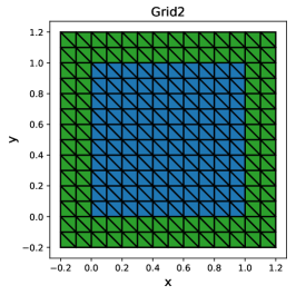
Figure 1: Three types of meshes used in the present work and their corresponding labels. In this figure, we use $\delta=0.2$, and decomposition of $\Omega_{\delta}$ into $\Omega$ and $\Gamma^{\text{nl}}$ is illustrated with color. Gmsh is utilized for generating unstructured meshes [GR09].

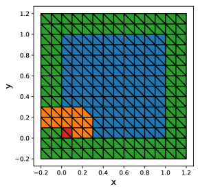
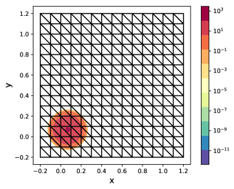
Figure 2: Left: reference elements $T_{1}$ (red), and elements $T_{2}$ (orange), participating in the pre-computation of the integrals. Note that only half of the elements in the proximity of the reference cell need to be considered owing to the symmetry of the bilinear form with respect to the change of the integration variables $x\leftrightarrow x^{\prime}$. Right: contour plot of $A_{\delta}(|\cdot-x|)$ for $x$ located at the barycenter of one of the reference elements. $\delta=0.2$ and $s=1/3$ is used.

Functions in $\mathcal{U}$ will be approximated with continuous piecewise-linear polynomials $u^{h}\in\mathcal{U}^{h}=\{\,v^{h}\in\mathcal{U}\cap C^{0}(\bar{\Omega}_{\delta}):v^{h}|_{T}\text{\ is a linear polynomial},\forall T\in\Omega_{\delta}^{h}\,\}$. Naturally we put $\mathcal{U}^{h}_{0}=\mathcal{U}^{h}\cap\mathcal{U}_{0}$, which leads us to the following discrete variational principle (system of linear algebraic equations): find $u_{h}\in\mathcal{U}^{h}_{0}$, such that

$$a_{\delta,\kappa}(u_{h},v_{h})=\ell(v_{h}),\quad\forall v_{h}\in\mathcal{U}_{0}^{h}.$$ (22)

Assembly process for the right hand side of this system is completely standard, whereas in order to assemble the left hand side of this system we need to loop over all pairs $(T_{1},T_{2})\in\Omega_{\delta}^{h}\times\Omega_{\delta}^{h}$ of elements in the mesh, which are not further than the distance of $2\delta$ from each other, and compute the local integral contribution to $a_{\delta,\kappa}(u_{h},v_{h})$, that is, the integral over $T_{1}\times T_{2}$. Note that when $\bar{T}_{1}\cap\bar{T}_{2}\neq\emptyset$, the integrand is unbounded; even when $\bar{T}_{1}\cap\bar{T}_{2}=\emptyset$ the integrand is not a polynomial function. In our implementation we utilize the quadratures described in [CvPS15], which are taylored for a nearly identical situation. In order to avoid commiting a variational crime by not integrating the bilinear form precisely, we first estimate how many quadrature points we need for the accurate integration; the results are reported in Fig. 3. Despite the fact that the assumptions imposed in [CvPS15] are not always satisfied we observe exponential convergence of the quadratures. However, note the unusial scaling of the $x$-axis; in the most singular case $k=2$ corresponding to $T_{1}=T_{2}$ we need approximately $15^{5}=759375$ quadrature points (when using Gauss–Jacobi quadrature in the singular direction, see [CvPS15] for details) to achieve nearly full IEEE double precision accuracy before the round off errors start to play a role!

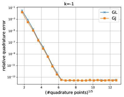
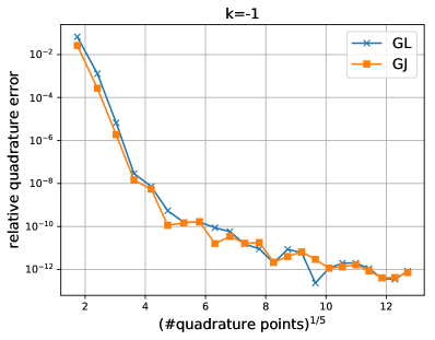
(a)	(b)
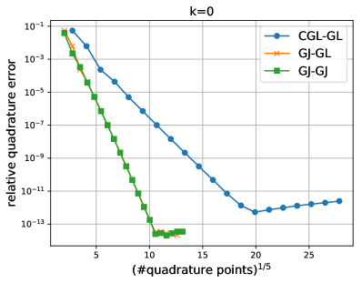
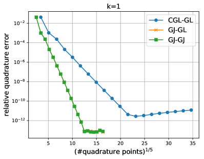
(c)	(d)
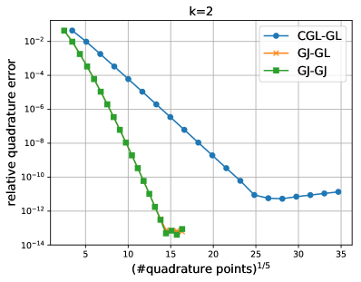
(e)

Figure 3: Verification of the exponential convergence rate of the quadratures [CvPS15], which we use for computing elemental stiffness matrices; $s=1/3$ in this simulation. $k$ is the dimension of the intersection $\bar{T}_{1}\cap\bar{T}_{2}$; $k=-1$ means $\bar{T}_{1}\cap\bar{T}_{2}=\emptyset$ and therefore the integrand is regular; see [CvPS15] for details. (a): $k=-1$ and $\operatorname{diam}(\bar{T}_{1}\cup\bar{T}_{2})<\delta$; (b): $k=-1$ and $\operatorname{diam}(\bar{T}_{1}\cup\bar{T}_{2})>\delta$; (c): $k=0$; (d): $k=1$; (e): $k=2$.

Because of such a high cost of elemental integration, and because the number of integrals in a quasi-uniform grid grows as $O(\delta^{n}h^{-2n})$, we focus on regular grids (see Fig. 1). In this setting we only need to evaluate integrals for a fixed ‘‘reference’’ $T_{1}$ and varying $T_{2}$, thereby bringing the number of integrals down to $O(\delta^{n}h^{-n})$ as shown in Fig. 2. Even with this preprocessing, both the work and memory requirements for the global matrix assembly scale as $O(\delta^{n}h^{-2n})$. Putting this into perspective, for Grid2 with $h=2^{1/2}/320$ (i.e., each side of the unit square $\Omega$ is discretized with $320$ elements) we need approximately $4.7$Mb to store the precomputed integrals and approximately $3.87\cdot 10^{3}$Mb to store the assembled matrix. Direct solver such as UMFPACK [Dav04] quickly run out of memory for problems with $\delta=0.1$, and we switch to CG-accelerated Ruge–Stuben AMG solver PyAMG [OS18] (even smoothed aggregation is too much memory and computationally demanding).

5.1.1 $h$-convergence test

In order to test the code, we use the method of manufactured solutions, see e.g. [Roa02]. We put $\delta=0.1$, $s\in\{1/3,2/3\}$, $\kappa\equiv 1$, and let the analytical solution to be $u_{\text{ana}}(x,y)=[x(1-x)y(1-y)]^{2}\sin(2\pi(x+y^{2}))$, when $x,y\in\Omega$, and zero otherwise. The corresponding right hand side can be (numerically) computed as

$$f(x,y)=-2\lim_{\epsilon\to 0}\int_{\epsilon}^{\delta}\int_{0}^{2\pi}A_{\delta}(r)\frac{u_{\text{ana}}(x+r\cos(\theta),y+r\sin(\theta))-u_{\text{ana}}(x,y)}{r}\,\mathrm{d}\theta\,\mathrm{d}r,$$ (23)

which is evaluated using the standard adaptive quadrature package in SciPy. The results of this test are shown in Fig. 4. In both cases we do observe convergence, although it is difficult to say whether we reach the asymptotic convergence rate (we run the simulations until we run out of memory), or indeed whether the adaptive quadratures evaluate (23) accurately enough.

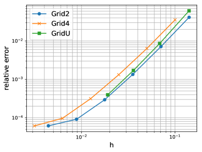
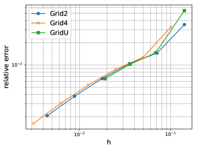
Figure 4: Verification of convergence of the discretization (and the numerical implementation) with respect to $h$-refinement. Left: $s=1/3$, right: $s=2/3$. The relative error is measured with respect to $L^{2}(\Omega_{\delta})$ norm.

5.1.2 ‘‘$\Gamma$-convergence’’ test

Another test we perform is that of ‘‘numerical $\Gamma$-convergence’’, that is, we try to illustrate Proposition 11. Namely we put $s=1/3$, $\rho(x,y)=\underline{\rho}+(\overline{\rho}-\underline{\rho})\exp\{-[(x-m_{x})^{2}+(y-m_{y})^{2}]/\sigma\}$ with $(m_{x},m_{y})=(1/2,2/3)$ and $\sigma=0.1$, and $\kappa$ computed from $\rho$ using the SIMP model with $p=2$, $u_{\text{ana}}(x,y)=\sin(2\pi x)\sin(\pi y)$, for $x,y\in\Omega$, and zero otherwise. We compute $f=-\operatorname{div}[\rho^{p}\nabla u_{\text{ana}}]$, and solve a variety of non-local problems with varying $\delta$ and $h$ on Grid2. The results are summarized in Fig. 5. The main observation is that the quantity $e(\delta)=\|u_{\text{ana}}-\lim_{h\to 0}u_{\delta,h}\|_{L^{2}(\Omega)}$, where $u_{\delta,h}$ is the numerical solution to the discretized non-local problem (22), appears to be decreasing with $\delta$. Unsurprisingly, one needs finer resolution meshes to resolve non-local problems with smaller values of $\delta$.

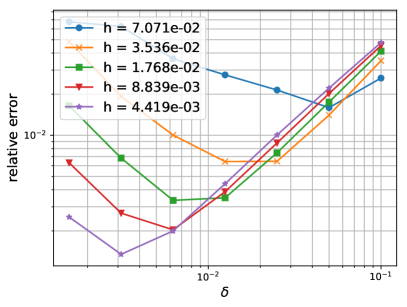
Figure 5: Numerical verification of $\Gamma$-convergence. The error is measured as $L^{2}(\Omega)$-norm of the difference between the numerical solution of the non-local problem and the analytical solution of the local problem.

5.2 Solving the optimization problem

In our implementation we solve a discretized version of the optimization problem (14) with a tiny discrepancy: instead of the constraint $\int_{\Omega}\rho(x)\,\mathrm{d}x\leq\gamma|\Omega|$ in (13) we have implemented the constraint $\int_{\Omega_{\delta}}\rho(x)\,\mathrm{d}x\leq\gamma|\Omega|$. We focus exclusively on compliance minimization, that is, $J(\rho,u)=\ell(u)$, and we employ the so-called optimality criterion (OC) scheme for solving these problems. This choice is primarily owing to the popularity of OC in the topology optimization community, and any other gradient-based non-linear constrained optimization algorithm could be utilized in its place. Within the OC scheme, given a current material distribution $\rho_{k}$ we first compute the corresponding state $u_{\rho_{k}}$ by solving the discretized system (22), and then the derivatives of non-local compliance $\mathfrak{c}_{\delta}$ as

$$\mathfrak{c}_{\delta}^{\prime}(\rho_{k};\xi)=-\frac{p}{2}\int_{\Omega_{\delta}}\int_{\Omega_{\delta}}[\rho_{k}^{p/2-1}(x)\rho_{k}^{p/2}(x^{\prime})\xi(x)+\rho_{k}^{p/2}(x)\rho_{k}^{p/2-1}(x^{\prime})\xi(x^{\prime})]A_{\delta}(|x-x^{\prime}|)\frac{(u_{\rho_{k}}(x)-u_{\rho_{k}}(x^{\prime}))^{2}}{|x-x^{\prime}|^{2}}\,\mathrm{d}x^{\prime}\,\mathrm{d}x.$$

The new material distribution is defined by a simple pointwise update scheme

$$\rho_{k+1}=\pi_{B_{k}}[\rho_{k}(-\nabla\mathfrak{c}_{\delta}(\rho_{k})/\lambda_{k+1})^{\xi}],$$

where $\pi_{B_{k}}[\cdot]$ is a projection operator onto a closed, convex, and non-empty set $B_{k}=\{\,\rho\in L^{2}(\Omega_{\delta})\mid\max[\underline{\rho},(1-\eta)\rho_{k}]\leq\rho\leq\min[\overline{\rho},(1+\eta)\rho_{k}]\,\}$, and $\eta>0$ and $\xi\in(0,1)$ are trust-region like and damping parameters, respectively, and $\nabla\mathfrak{c}_{\delta}(\rho_{k})$ is $L^{2}(\Omega_{\delta})$ representation of the directional derivatives $\mathfrak{c}_{\delta}^{\prime}(\rho_{k};\xi)$. Finally, $\lambda_{k+1}$ is computed by finding the root of the equation $\int_{\Omega_{\delta}}\rho_{k+1}(x)\,\mathrm{d}x=\gamma|\Omega|$ using, for example, the bisection algorithm. We put $\eta=0.2$, $\xi=0.5$, and stop the algorithm when $\|\rho_{k+1}-\rho_{k}\|_{L^{2}(\Omega_{\delta})}<10^{-4}$. For more details see [BS03].

5.2.1 Convex case: $p=1$

In the the ‘‘easy’’ convex case corresponding to $p=1$ we can expect that the optimization algorithm computes approximations to (discretized approximations of) globally optimal solutions. The computed local conductivities $\kappa^{\text{loc}}=\rho$ and the corresponding states for several values of $\delta$ are shown in Figure 6. Note that in this case the local compliance minimization problem (5) admits globally optimal solutions, which is also shown in Figure 6 with the corresponding state. The qualitative resemblance between the solutions to the non-local and local problems is clear from these pictures. Additionally, we seem to have a quantitative connection between the two problems, illustrated in Table 1.

Note that the number of optimization iterations needed to solve the problem is virtually independent from the value of the non-local horizon $\delta$ or size of the mesh $h$. Still, each iteration of the optimization algorithm, which requires solving the discretized state equations, becomes significantly more costly for larger $\delta>0$.

$\delta$	$h$	$J^{*}$	$N$
$0.2$	$3.54\cdot 10^{-2}$	$9.0727\cdot 10^{-2}$	$26$
$0.2$	$1.77\cdot 10^{-2}$	$9.1778\cdot 10^{-2}$	$27$
$0.2$	$8.84\cdot 10^{-3}$	$9.2408\cdot 10^{-2}$	$27$
$0.2$	$4.42\cdot 10^{-3}$	$9.2798\cdot 10^{-2}$	$27$
$0.1$	$3.54\cdot 10^{-2}$	$7.8627\cdot 10^{-2}$	$28$
$0.1$	$1.77\cdot 10^{-2}$	$7.9479\cdot 10^{-2}$	$32$
$0.1$	$8.84\cdot 10^{-3}$	$7.9930\cdot 10^{-2}$	$32$
$0.1$	$4.42\cdot 10^{-3}$	$8.0218\cdot 10^{-2}$	$32$
$0.05$	$3.54\cdot 10^{-2}$	$7.3251\cdot 10^{-2}$	$29$
$0.05$	$1.77\cdot 10^{-2}$	$7.3896\cdot 10^{-2}$	$34$
$0.05$	$8.84\cdot 10^{-3}$	$7.4276\cdot 10^{-2}$	$36$
$0.05$	$4.42\cdot 10^{-3}$	$7.4484\cdot 10^{-2}$	$35$
$0$	$3.13\cdot 10^{-3}$	$6.9460\cdot 10^{-2}$	$38$

Table 1: Summary of the results for the convex case $p=1$. $J^{*}$: optimal value; $N$: number of OC iterations. $\delta=0$ corresponds to the limiting local model (solved using a separate code) which admits optimal solutions in the convex case $p=1$, see [CM70, BS03, All12].

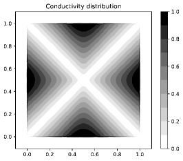
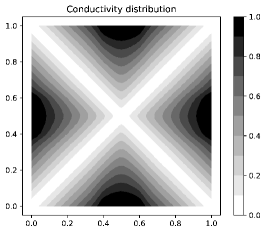
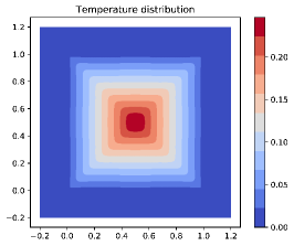
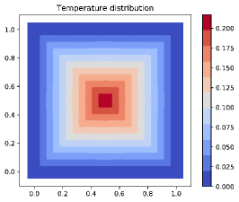
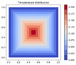
Figure 6: Pictures of the computed optimal designs for $p=1$. Top line: optimal design (conductivity distribution $\kappa^{\text{loc}}=\rho$), bottom line: corresponding optimal states. From left to right: $\delta=0.2$, $\delta=0.05$, $\delta=0$ (local problem). Note the slightly different color range and the presence of $\Gamma^{\text{nl}}$ for the nonlocal problems.

5.2.2 Nonconvex case: $p=2$

A significantly more interesting case, in view of the very different behaviour of the non-local and local problems, corresponds to the non-convex optimization problem (14) with $p=2$. In this case, for the local problem the intermediate values of the conductivity are effectively penalized by the underlying physics and one can expect the computed optimized conductivity distribitions to be of ‘‘bang-bang’’ structure, assuming either the lowest or the highest possible values of conductivity everywhere. Note also that in this case the local optimization problem (5) does not admit optimal solutions, and therefore we have no local solution to compare with.

The computed local conductivities $\kappa^{\text{loc}}=\rho^{p}$ and the corresponding states for several values of $\delta$ are shown in Figure 7. They agree with our expectations. One can also note that for smaller $\delta$ the computed conductivity distributions display smaller features and progressively more oscillatory character. Indeed, in the case of the local problem, minimizing sequences consist of conductivities, which are locally highly oscillatory (periodic) and can be mathematically understood as converging to composite materials, see [BS03, All12]. Quantitative information about these solutions is shown in Table 2. Note that for smaller $\delta$ the optimization algorithm requires significantly more iterations to converge (which does not mean that it is more difficult to solve, as each iteration is less computationally expensive in this case).

The non-existence of optimal solutions for the local compliance minimization problem manifests itself numerically as ‘‘mesh-dependence’’ of optimal designs, where progressively more oscillatory conductivity distributions are encountered as one refines the computational mesh. This is often used as an ‘‘engineering’’ test of existence of optimal solutions for a given problem. The optimal conductivity distributions corresponding to $\delta=0.2$ and a range of discretization levels is shown in Figure 8. Indeed, one can recognize the sequence of convergent shapes as the discretization gets finer and finer. Again, this example works by pure coincidence: indeed as the problem is non-convex the optimization algorithm may end up in different local minima at different discretization levels, and indeed we have observed such behavior for other values of $\delta$.

Finally, we perform a ‘‘cross-check’’ of the computed non-local designs by evaluating all computed designs for all values of $\delta$. We expect (but of course cannot guarantee this, as we can only hope to find locally optimal solutions and not global ones) that the distribution optimized for a specific value of $\delta$ would outperform other designs computed for different values of $\delta$. The results of this test are shown in Table 3. Indeed, our expectations are confirmed: within each row the diagonal element is the smallest one.

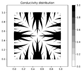
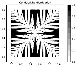
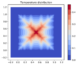
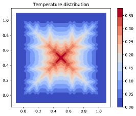
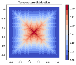
Figure 7: Pictures of the computed optimal designs for $p=2$. Top line: optimal design (conductivity distribution $\kappa^{\text{loc}}=\rho^{2}$), bottom line: corresponding optimal states. From left to right: $\delta=0.2$, $\delta=0.1$, $\delta=0.05$. Note the slightly different color range and the presence of $\Gamma^{\text{nl}}$ for the nonlocal problems.

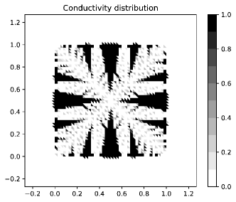
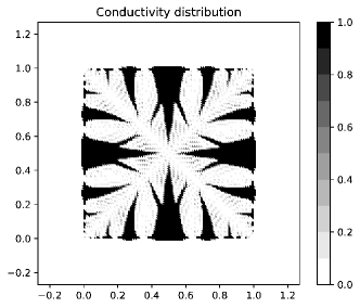
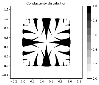
Figure 8: ‘‘Mesh-independence’’ test (owing to the non-convexity of the problem we cannot guarantee that the optimization algorithm converges to the ‘‘same’’ local minimum on different discretizations). Conductivity distributions $\kappa^{\text{loc}}=\rho^{2}$ are shown. We put $p=2$, $\delta=0.2$, and $h\in\{3.54\cdot 10^{-2},1.77\cdot 10^{-2},8.84\cdot 10^{-3},4.42\cdot 10^{-3}\}$.

$\delta$	$h$	$J^{*}$	$N$
$0.2$	$3.54\cdot 10^{-2}$	$1.6902\cdot 10^{-1}$	$1080$
$0.2$	$1.77\cdot 10^{-2}$	$1.7327\cdot 10^{-1}$	$1062$
$0.2$	$8.84\cdot 10^{-3}$	$1.7516\cdot 10^{-1}$	$1300$
$0.2$	$4.42\cdot 10^{-3}$	$1.7613\cdot 10^{-1}$	$1139$
$0.1$	$3.54\cdot 10^{-2}$	$1.2857\cdot 10^{-1}$	$514$
$0.1$	$1.77\cdot 10^{-2}$	$1.3242\cdot 10^{-1}$	$1116$
$0.1$	$8.84\cdot 10^{-3}$	$1.3480\cdot 10^{-1}$	$1395$
$0.1$	$4.42\cdot 10^{-3}$	$1.3560\cdot 10^{-1}$	$1521$
$0.05$	$3.54\cdot 10^{-2}$	$1.0721\cdot 10^{-1}$	$261$
$0.05$	$1.77\cdot 10^{-2}$	$1.1066\cdot 10^{-1}$	$790$
$0.05$	$8.84\cdot 10^{-3}$	$1.1139\cdot 10^{-1}$	$1358$
$0.05$	$4.42\cdot 10^{-3}$	$1.1185\cdot 10^{-1}$	$2394$

Table 2: Summary of the results for the non-convex case $p=2$. $J^{*}$: computed objective value; $N$: number of OC iterations.

Original $\delta$	$J$ for $\delta=0.05$	$J$ for $\delta=0.1$	$J$ for $\delta=0.2$
$0.05$	$\mathbf{1.1185\cdot 10^{-1}}$	$1.1724\cdot 10^{-1}$	$1.3225\cdot 10^{-1}$
$0.1$	$1.3954\cdot 10^{-1}$	$\mathbf{1.3560\cdot 10^{-1}}$	$1.4172\cdot 10^{-1}$
$0.2$	$1.9678\cdot 10^{-1}$	$1.8213\cdot 10^{-1}$	$\mathbf{1.7613\cdot 10^{-1}}$

Table 3: ‘‘Cross-checking’’ of the computed designs, $h=4.42\cdot 10^{-3}$ in all cases.

References

- [AB98] Giovanni Alberti and Giovanni Bellettini. A nonlocal anisotropic model for phase transitions. I. The optimal profile problem. Math. Ann., 310(3):527–560, 1998.
- [All12] Grégoire Allaire. Shape optimization by the homogenization method, volume 146. Springer Science & Business Media, 2012.
- [AM10] Burak Aksoylu and Tadele Mengesha. Results on nonlocal boundary value problems. Numer. Funct. Anal. Optim., 31(12):1301–1317, 2010.
- [AM15a] Fuensanta Andrés and Julio Muñoz. Nonlocal optimal design: a new perspective about the approximation of solutions in optimal design. Journal of Mathematical Analysis and Applications, 429(1):288–310, 2015.
- [AM15b] Fuensanta Andrés and Julio Muñoz. A type of nonlocal elliptic problem: Existence and approximation through a Galerkin–Fourier method. SIAM Journal on Mathematical Analysis, 47(1):498–525, 2015.
- [AM17] Fuensanta Andrés and Julio Muñoz. On the convergence of a class of nonlocal elliptic equations and related optimal design problems. Journal of Optimization Theory and Applications, 172(1):33–55, 2017.
- [AVMRTM10] Fuensanta Andreu-Vaillo, José M. Mazón, Julio D. Rossi, and J. Julián Toledo-Melero. Nonlocal diffusion problems, volume 165 of Mathematical Surveys and Monographs. American Mathematical Society, Providence, RI; Real Sociedad Matemática Española, Madrid, 2010.
- [BBM01] Jean Bourgain, Haim Brezis, and Petru Mironescu. Another look at Sobolev spaces. In Optimal control and partial differential equations, pages 439–455. IOS, Amsterdam, 2001.
- [BE19] José C. Bellido and Anton Evgrafov. A simple characterization of -convergence for a class of nonlocal problems. arXiv e-prints, page arXiv:1903.11585, Mar 2019.
- [BK88] Martin Philip Bendsøe and Noboru Kikuchi. Generating optimal topologies in structural design using a homogenization method. Computer methods in applied mechanics and engineering, 71(2):197–224, 1988.
- [BMC14] José C. Bellido and Carlos Mora-Corral. Existence for nonlocal variational problems in peridynamics. SIAM J. Math. Anal., 46(1):890–916, 2014.
- [BMCP15] José C. Bellido, Carlos Mora-Corral, and Pablo Pedregal. Hyperelasticity as a -limit of peridynamics when the horizon goes to zero. Calc. Var. Partial Differential Equations, 54(2):1643–1670, 2015.
- [Bou01] Blaise Bourdin. Filters in topology optimization. International journal for numerical methods in engineering, 50(9):2143–2158, 2001.
- [Bra02] Andrea Braides. -convergence for beginners, volume 22 of Oxford Lecture Series in Mathematics and its Applications. Oxford University Press, Oxford, 2002.
- [Bre10] Haim Brezis. Functional analysis, Sobolev spaces and partial differential equations. Springer Science & Business Media, 2010.
- [BS03] MP Bendøse and Ole Sigmund. Topology Optimization: Theory, Methods and Applications. ISBN: 3-540-42992-1. Springer, 2003.
- [BV16] Claudia Bucur and Enrico Valdinoci. Nonlocal diffusion and applications, volume 20 of Lecture Notes of the Unione Matematica Italiana. Springer, [Cham]; Unione Matematica Italiana, Bologna, 2016.
- [CCEM07] C. Cortázar, J. Coville, M. Elgueta, and S. Martínez. A nonlocal inhomogeneous dispersal process. J. Differential Equations, 241(2):332–358, 2007.
- [CM70] Jean Céa and Kazimierz Malanowski. An example of a max-min problem in partial differential equations. SIAM Journal on Control, 8(3):305–316, 1970.
- [CvPS15] Alexey Chernov, Tobias von Petersdorff, and Christoph Schwab. Quadrature algorithms for high dimensional singular integrands on simplices. Numerical algorithms, 70(4):847–874, 2015.
- [Dav04] Timothy A Davis. Algorithm 832: Umfpack v4. 3—an unsymmetric-pattern multifrontal method. ACM Transactions on Mathematical Software (TOMS), 30(2):196–199, 2004.
- [DG14] Marta D’Elia and Max Gunzburger. Optimal distributed control of nonlocal steady diffusion problems. SIAM J. Control Optim., 52(1):243–273, 2014.
- [DG16] M. D’Elia and M. Gunzburger. Identification of the diffusion parameter in nonlocal steady diffusion problems. Appl. Math. Optim., 73(2):227–249, 2016.
- [DNPV12] Eleonora Di Nezza, Giampiero Palatucci, and Enrico Valdinoci. Hitchhiker’s guide to the fractional Sobolev spaces. Bulletin des Sciences Mathématiques, 136(5):521–573, 2012.
- [Du19] Qiang Du. Nonlocal modeling, analysis and computation. SIAM, 2019.
- [EB18] Anton Evgrafov and José C. Bellido. From non-local Eringen’s model to fractional elasticity. Mathematics and Mechanics of Solids, 2018.
- [EB19] Anton Evgrafov and José C Bellido. Sensitivity filtering from the non-local perspective. Structural and Multidisciplinary Optimization, 2019.
- [Eri02] A Cemal Eringen. Nonlocal continuum field theories. Springer Science & Business Media, 2002.
- [EW07] Etienne Emmrich and Olaf Weckner. On the well-posedness of the linear peridynamic model and its convergence towards the Navier equation of linear elasticity. Commun. Math. Sci., 5(4):851–864, 2007.
- [FBRS17] Julián Fernández Bonder, Antonella Ritorto, and Ariel Martin Salort. -convergence result for nonlocal elliptic-type problems via Tartar’s method. SIAM J. Math. Anal., 49(4):2387–2408, 2017.
- [FBRS18] Julián Fernández Bonder, Antonella Ritorto, and Ariel Martin Salort. A class of shape optimization problems for some nonlocal operators. Adv. Calc. Var., 11(4):373–386, 2018.
- [Fif03] Paul Fife. Some nonclassical trends in parabolic and parabolic-like evolutions. In Trends in nonlinear analysis, pages 153–191. Springer, Berlin, 2003.
- [GO08] Guy Gilboa and Stanley Osher. Nonlocal operators with applications to image processing. Multiscale Model. Simul., 7(3):1005–1028, 2008.
- [GR09] Christophe Geuzaine and Jean-François Remacle. Gmsh: A 3-d finite element mesh generator with built-in pre-and post-processing facilities. International journal for numerical methods in engineering, 79(11):1309–1331, 2009.
- [Kun75] IA Kunin. Теория упругих сред с микроструктурой: нелокальная теория упругости (Theory of elastic bodies with microstructure: nonlocal theory of elasticity). Издательство Наука (Izd Nauka), Moscow (in Russian), 1975.
- [MD15] Tadele Mengesha and Qiang Du. On the variational limit of a class of nonlocal functionals related to peridynamics. Nonlinearity, 28(11):3999–4035, 2015.
- [MO17] E. Madenci and E. Oterkus. Handbook of Nonlocal Continuum Mechanics for Materials and Structures. Springer, [Cham], 2017.
- [MT97] François Murat and Luc Tartar. -convergence. In Topics in the mathematical modelling of composite materials, volume 31 of Progr. Nonlinear Differential Equations Appl., pages 21–43. Birkhäuser Boston, Boston, MA, 1997.
- [Mur78] François Murat. Compacité par compensation. Ann. Scuola Norm. Sup. Pisa Cl. Sci. (4), 5(3):489–507, 1978.
- [OS18] L. N. Olson and J. B. Schroder. PyAMG: Algebraic multigrid solvers in Python v4.0, 2018. Release 4.0.
- [Ped16] Pablo Pedregal. Optimal design through the sub-relaxation method, volume 11 of SEMA SIMAI Springer Series. Springer, [Cham], 2016. Understanding the basic principles.
- [Pon04a] Augusto C Ponce. An estimate in the spirit of Poincaré’s inequality. Journal of the European Mathematical Society, 6(1):1–15, 2004.
- [Pon04b] Augusto C. Ponce. A new approach to Sobolev spaces and connections to -convergence. Calc. Var. Partial Differential Equations, 19(3):229–255, 2004.
- [Roa02] Patrick J Roache. Code verification by the method of manufactured solutions. Journal of Fluids Engineering, 124(1):4–10, 2002.
- [Rog91] Robert C. Rogers. A nonlocal model for the exchange energy in ferromagnetic materials. J. Integral Equations Appl., 3(1):85–127, 1991.
- [Roy88] H. L. Royden. Real analysis. Macmillan Publishing Company, New York, third edition, 1988.
- [Rud87] Walter Rudin. Real and complex analysis. McGraw-Hill Book Co., New York, third edition, 1987.
- [Sig97] Ole Sigmund. On the design of compliant mechanisms using topology optimization. Journal of Structural Mechanics, 25(4):493–524, 1997.
- [Sil00] Stewart A Silling. Reformulation of elasticity theory for discontinuities and long-range forces. Journal of the Mechanics and Physics of Solids, 48(1):175–209, 2000.
- [Spa67] Sergio Spagnolo. Sul limite delle soluzioni di problemi di Cauchy relativi alléquazione del calore. Annali della Scuola Normale Superiore di Pisa-Classe di Scienze, 21(4):657–699, 1967.
- [Tar79a] L. Tartar. Compensated compactness and applications to partial differential equations. In Nonlinear analysis and mechanics: Heriot-Watt Symposium, Vol. IV, volume 39 of Res. Notes in Math., pages 136–212. Pitman, Boston, Mass.-London, 1979.
- [Tar79b] L. Tartar. Estimation de coefficients homogénéisés. In Computing methods in applied sciences and engineering (Proc. Third Internat. Sympos., Versailles, 1977), I, volume 704 of Lecture Notes in Math., pages 364–373. Springer, Berlin, 1979.
- [Voy14] G. Voyiadjis, editor. Peridynamic Theory and Its Applications. Springer, [New York], 2014.
- [YSS18] F. Wang Y. Suna and O. Sigmund. On the non-optimality of tree structures for heat conduction. International Journal of Heat and Mass Transfer, 122:660–680, 2018.