An exact firing rate model reveals the differential effects of chemical versus electrical synapses in spiking networks

Abstract

Chemical and electrical synapses shape the dynamics of neuronal networks. Numerous theoretical studies have investigated how each of these types of synapses contributes to the generation of neuronal oscillations, but their combined effect is less understood. This limitation is further magnified by the impossibility of traditional neuronal mean-field models —also known as firing rate models, or firing rate equations— to account for electrical synapses. Here we introduce a novel firing rate model that exactly describes the mean field dynamics of heterogeneous populations of quadratic integrate-and-fire (QIF) neurons with both chemical and electrical synapses. The mathematical analysis of the firing rate model reveals a well-established bifurcation scenario for networks with chemical synapses, characterized by a codimension-2 Cusp point and persistent states for strong recurrent excitatory coupling. The inclusion of electrical coupling generally implies neuronal synchrony by virtue of a supercritical Hopf bifurcation. This transforms the Cusp scenario into a bifurcation scenario characterized by three codimension-2 points (Cusp, Takens-Bogdanov, and Saddle-Node Separatrix Loop), which greatly reduces the possibility for persistent states. This is generic for heterogeneous QIF networks with both chemical and electrical coupling. Our results agree with several numerical studies on the dynamics of large networks of heterogeneous spiking neurons with electrical and chemical coupling.

I Introduction

Collective oscillations and synchrony are prominent features of neuronal circuits, and are fundamental for the well-timed coordination of neuronal activity. Such oscillations are profoundly shaped by the presence of chemical synapses Wang (2010). An increasing number of experimental studies indicate both the prevalence and functional importance of electrical synapses (formed by gap junctions between neurons) in many diverse regions of central nervous systems, especially in inhibitory interneurons Nagy et al. (2018); Connors (2017); Traub et al. (2018). Electrical synapses participate in mediating synchronization of neuronal network activity Bennett and Zukin (2004); Connors and Long (2004), suggesting that electrical interaction may be interrelated with the generation of oscillations via chemical transmission.

The mechanisms by which chemical synapses mediate large-scale synchronous activity have been extensively investigated, see e.g. Wang (2010); Whittington et al. (2000). However, only a few studies addressed the synchronization of large networks in which neurons are not only interacting via excitation and/or inhibition, but also via electrical synapses  Kopell and Ermentrout (2004); Pfeuty et al. (2007); Ermentrout (2006); Viriyopase et al. (2016); Holzbecher and Kempter (2018); Guo et al. (2012); Tchumatchenko and Clopath (2014); Lewis and Rinzel (2003); Chow and Kopell (2000); Ostojic et al. (2009); Pfeuty et al. (2003); Coombes (2008); Mancilla et al. (2007). This limited theoretical progress for networks of electrically coupled neurons, compared to chemically coupled networks, is magnified due to the technical challenges faced when developing simplified mean field models —often called firing rate models, or firing rate equations (FRE)— for networks involving electrical synapses. While firing rate models turned out to be very useful to explain key aspects of the dynamics of spiking neuron networks with chemical synapses  Wilson and Cowan (1972); Dayan and Abbott (2001); Ermentrout and Terman (2010); Hopfield (1984); Mongillo et al. (2008); Ben-Yishai et al. (1995); Hansel and Sompolinsky (1998); Tabak et al. (2000); Rankin et al. (2015); Martí and Rinzel (2013); Tsodyks M. (1998); Roxin et al. (2005); Roxin and Montbrió (2011), it remains an open question whether there are similar simplified mean field theories for networks involving electrical interactions.

Recently, a novel method has been found to exactly derive FRE for populations of heterogeneous quadratic integrate-and-fire (QIF) neurons with chemical coupling Montbrió et al. (2015). The method, related to the so-called Ott-Antonsen ansatz Ott and Antonsen (2008, 2009); Ott et al. (2011); Pikovsky and Rosenblum (2008); Marvel et al. (2009); Pikovsky and Rosenblum (2011); Pietras and Daffertshofer (2016), allows to obtain exact, low-dimensional firing rate equations for ensembles of QIF neurons, see also Luke et al. (2013); So et al. (2014); Laing (2014). The FRE for QIF neurons have been used to investigate numerous problems regarding the dynamics of networks of chemically coupled QIF neurons  Pazó and Montbrió (2016); Ratas and Pyragas (2016); Roulet and Mindlin (2016); Devalle et al. (2018, 2017); Esnaola-Acebes et al. (2017); Ratas and Pyragas (2017); Dumont et al. (2017); Byrne et al. (2017); Laing (2018); Schmidt et al. (2018); Ratas and Pyragas (2018); di Volo and Torcini (2018); Dumont and Gutkin (2019); Akao et al. (2019); Bi et al. (2019); Coombes and Byrne (2019); Keeley et al. (2019); Byrne et al. (2019); Boari et al. (2019). Remarkably, previous work has also sought to apply this approach to networks with both chemical and electrical coupling Laing (2015). However, in Laing (2015), the electrical coupling has been treated by making use of an approximation which renders the resulting FRE analytically intractable. We build on this previous work and derive a set of FRE for networks with chemical and electrical coupling, but without the need for any approximation. The resulting system is not only analytically tractable but also allows, in a unified framework, for carrying out a complete analysis of the possible dynamics and bifurcations of networks with mixed chemical and electrical synapses. In Appendix B we show that our exact FRE are recovered by appropriately relaxing the approximation invoked in Laing (2015).

The structure of the paper is as follows: In Section II, we describe the spiking neuron network under investigation, and briefly illustrate the impact of electrical coupling in the dynamics of two nonidentical QIF neurons. In Section III, we introduce the FRE corresponding to the thermodynamic limit of the QIF network. The detailed derivation is performed in Appendix A. In Section IV, we perform a comparative analysis of the fixed points and their bifurcations in networks with electrical coupling vs. networks with chemical coupling. Finally, we investigate the dynamics of a QIF network with both electrical and chemical synapses and demonstrate that the presence of electrical coupling critically determines the bifurcation scenario of the neuronal network. Finally, we discuss our results in Section V.

II Quadratic integrate-and-fire neurons with electrical and chemical synapses

We consider a large population of globally electrically and chemically-coupled QIF neurons, with membrane potentials $\{V_{j}\}_{j=1,\dots,N}$ and $N\!\gg\!1$. Their dynamics reads

$$\tau\dot{V}_{j}=V_{j}^{2}+\eta_{j}+g(v-V_{j})+J\tau s,$$ (1)

where $\tau$ denotes the cells’ common membrane time constant, and parameter $\eta_{j}$ represents an external input current flowing into cell $j$. To model the action potential, the continuous dynamics Eq. (1) is supplemented by a discrete resetting rule. Here, we assume that if $V_{j}$ reaches infinity, neuron $j$ emits a spike and its membrane potential is reset to minus infinity . The mean membrane voltage

$$v=\frac{1}{N}\sum_{k=1}^{N}V_{k},$$

to which all cells are diffusively coupled with strength $g\geq 0$, mediates the electrical coupling. The constant $J$ quantifies the coupling strength of chemical synapses. The coupling via chemical synapses is mediated by the mean synaptic activation function

$$s(t)=\frac{1}{N}\sum_{j=1}^{N}\frac{1}{\tau_{s}}\int\limits_{t-\tau_{s}}^{t}\sum_{k}\delta\!\left(t^{\prime}-t_{j}^{k}\right)\,dt^{\prime},$$ (2)

where $t_{j}^{k}$ denotes the time of the $k$-th spike of the $j$-th neuron, $\delta(t)$ is the Dirac delta function, and $\tau_{s}$ is a synaptic time constant  . The synaptic weight $J$ can be positive or negative depending on whether the chemical synapses are excitatory or inhibitory, respectively

In the absence of coupling, $J=g=0$, the QIF neurons are either quiescent ($\eta_{i}<0$), or oscillatory ($\eta_{i}>0$) with frequency

$$f_{i}=\frac{1}{\tau\pi}\sqrt{\eta_{i}}.$$ (3)

These two dynamical regimes of individual neurons are connected by a saddle-node on the invariant circle (SNIC) bifurcation, which occurs when $\eta_{i}=0$, with $f_{i}=0$.

Electrical coupling tends to equalize the membrane potentials of the neurons they connect and may favor synchrony. Yet, if a large fraction of cells in the network is quiescent, gap junctions may suppress oscillations and neural synchrony. Next we illustrate this phenomenon for two nonidentical QIF neurons that are coupled via a gap junction . The results of this analysis will later be useful to understand some aspects of the dynamics of a large network of electrically coupled QIF neurons.

II.1 Strong coupling limit of two electrically coupled QIF neurons

We consider a network of $N=2$ nonidentical QIF neurons with dynamics Eq. (1). The neurons are coupled via gap junctions only, i.e. $J=0$ but $g>0$. We are interested in the strong coupling limit $g\gg 0$ when $\eta_{1}>0$ and $\eta_{2}<0$. In Fig. 1 we depict the corresponding time series of cell 1 (panel a) and cell 2 (panel b). Black thin curves correspond to the dynamics of the uncoupled ($g=0$) cells: cell 1 fires periodically, while cell 2 remains quiescent. When the neurons are electrically coupled (red curves), the membrane voltage of cell 2 displays a series of so-called ‘spikelets’ . Moreover, the electrical interaction brings cell 1 closer to its firing threshold and, hence, its frequency $f_{1}$ is reduced. When $g$ is increased further, cell 1 becomes quiescent (blue thick curves).

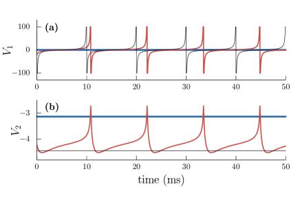
Figure 1: Strong electrical coupling suppresses oscillatory activity for negative mean currents, $\bar{\eta}<0$. The panels show the time series of the membrane voltages of $N=2$ electrically coupled QIF neurons. (a) Self-oscillatory neuron with $\eta_{1}=\pi^{2}$; (b) Quiescent neuron with $\eta_{2}=-2\pi^{2}$. The two neurons are either uncoupled (black thin curves, $g=0$), weakly coupled (red curves, $g=1$), or strongly coupled (blue thick curves, $g=6$). We used $\tau=10$ ms and $J=0$.

Although analyzing the dynamics of the two cells for arbitrary coupling strength $g$ is a challenge, there exists a simple and general result valid in the large $g$ limit, and of relevance for the large-$N$ analysis carried out below. Indeed, for large $g$, the dynamics of the $N=2$ network simply depends on the sign of the mean current Pazó and Montbrió (2006)

$$\bar{\eta}=\frac{\eta_{1}\!+\!\eta_{2}}{2}.$$

For $\bar{\eta}>0$, the quiescent cell eventually becomes self-oscillatory as $g$ is increased from zero. By contrast, for $\bar{\eta}<0$, the oscillatory cell eventually turns quiescent in the strong coupling limit; see the blue lines in Fig. 1 .

III Firing Rate Model

In the following, we introduce the FRE corresponding to the thermodynamic limit of Eqs. (1). The detailed derivation of the model closely follows the lines of Montbrió et al. (2015) and is given in Appendix A.

For $N\to\infty$, one can drop the indices in Eq. (1) and define a density function $\rho$ such that $\rho(V|\eta,t)~{}dV$ denotes the fraction of neurons with membrane potentials between $V$ and $V\!+\!dV$ and parameter $\eta$ at time $t$. In the limit of instantaneous synaptic processing, i.e. for $\tau_{s}\to 0$, Eq. (2) reduces to $s(t)=r(t)$ with $r(t)$ being the population-mean firing rate. If the external currents are distributed according to a Lorentzian distribution centered around $\eta=\bar{\eta}$ with half-width $\Delta$,

$$L_{\Delta,\bar{\eta}}(\eta)=\frac{1}{\pi}\frac{\Delta}{(\eta-\bar{\eta})^{2}+\Delta^{2}},$$ (4)

we find that the asymptotic mean-field dynamics evolves according to the following FRE

$$\tau\dot{r} = \tfrac{\Delta}{\tau\pi}+2rv-gr,$$ (5a)

$$\tau\dot{v} = v^{2}+\bar{\eta}-(\pi\tau r)^{2}+J\tau r.$$ (5b)

The variables $r$ and $v$ are the mean firing rate and mean membrane potential, respectively. They determine the total voltage density for the network Eq. (1), which turns out to be a Lorentzian distribution centered at $v(t)$ and of half-width $\pi\tau r(t)$,

$$\rho(V,t)=\frac{1}{\pi}\frac{\pi\tau r(t)}{\left[V-v(t)\right]^{2}+\left[\pi\tau r(t)\right]^{2}}.$$ (6)

The structure of the FRE Eqs. (5) reveals an interesting feature: Electrical coupling is solely mediated by the firing rate through the negative feedback term $-gr$ in the $r$-dynamics Eq. (5a), and not by membrane potential differences  . That is, electrical coupling leads to a narrowing of the voltage distribution Eq. (6), i.e. a decrease in firing rate. This confirms our initial sketch that electrical coupling tends to equalize the neurons’ membrane potentials and, under suitable conditions, this may promote synchrony. By contrast, chemical coupling shifts the center of the distribution Eq. (6) of voltages via the feedback term $Jr$ in the $v$-dynamics Eq. (5b). The following phase plane and bifurcation analysis of the FRE (5) allows for understanding the collective dynamics of the QIF network.

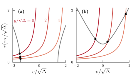
Figure 2: The sign of the mean current $\bar{\eta}$ determines the behavior of the fixed points of the FRE (5) with electrical coupling only, $J=0$. The panels show the nullclines of the FRE (5) with only electrical coupling ($J=0$) for negative ($\bar{\eta}/\Delta=-2$) and positive ($\bar{\eta}/\Delta=0.5$) values of $\bar{\eta}$ (panel a and b, respectively), and $g/\sqrt{\Delta}=0,2,4$. The black points correspond to the intersections of $r$-nullclines ($\dot{r}=0$, red) and $v$-nullclines ($\dot{v}=0$, gray) and are fixed points of Eqs. (5).

IV Analysis of the Firing Rate Equations

IV.1 Electrical vs. chemical coupling

In the absence of chemical coupling, our previous discussion of the case $N\!=\!2$ hints at two distinct dynamical regimes for positive and negative values of $\bar{\eta}$. With respect to the fixed points $(r_{*},v_{*})$ of the FRE (5) for $J=0$, we find the $v$-nullcline to be

$$\pi\tau r=\sqrt{v^{2}+\bar{\eta}}.$$

Note that if $\bar{\eta}$ is negative, there exists a range of ‘forbidden’ values of $v$. Fig. 2(a) shows the nullclines for $\bar{\eta}<0$ and for different values of the ratio $g/\sqrt{\Delta}$. Since the majority of the neurons are quiescent, an increase in coupling strength $g$ causes active neurons to reduce firing, which leads to a progressive decrease of the firing rate $r_{*}$. By contrast, in Fig. 2(b) the majority of the cells are self-oscillatory, $\bar{\eta}>0$, and strong electrical coupling forces quiescent neurons to fire. This yields an increase of $v_{*}$. Interestingly, the firing rate $r_{*}$ is a non-monotonic function of $g/\sqrt{\Delta}$: While $v_{*}$ remains negative, the voltages are pushed to subthreshold values, decreasing the firing rate. This behavior is reverted when $v_{*}$ becomes positive and all voltages are pushed towards values above the firing threshold. The different behaviors of Eqs. (5) with electrical coupling for positive and negative values of $\bar{\eta}$ are clearly revealed in the corresponding bifurcation diagrams shown in Figs. 3(a,c).

The case of networks with only chemical coupling, $g=0$, is simpler Montbrió et al. (2015). The bifurcation diagram depicted in Fig. 3(d) shows that $v_{*}$ remains always negative and converges asymptotically to zero as $J$ increases. The firing rate $r_{*}$, depicted in Fig. 3(b), also increases with $J$. For $\bar{\eta}<0$ and strong recurrent excitatory coupling, the system undergoes a cusp bifurcation and two saddle-node (SN) bifurcations are created. This implies the existence of a parameter regime where a persistent, high-activity state (stable focus) coexists with a low-activity state (stable node) —see Fig. 7(a), and  Montbrió et al. (2015). This coexistence between persistent and low-activity states also occurs in networks with electrical synapses, but it is located in a very small region of parameters as we show below, see Fig. 6(b).

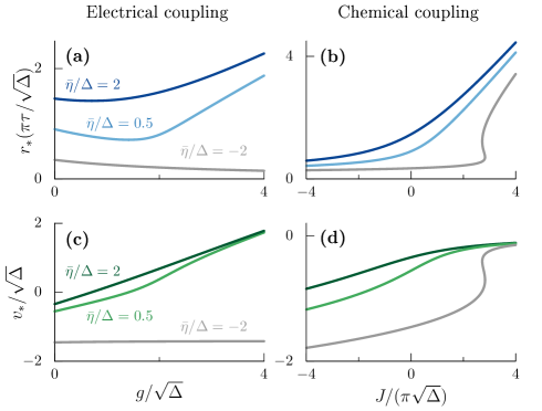
Figure 3: The bifurcation diagrams of the FRE (5) for networks with (left) electrical and (right) chemical coupling are qualitatively different. Top panels show the scaled firing rate $r_{*}/(\pi\tau\sqrt{\Delta})$ versus the ratio of (a) electrical $g/\sqrt{\Delta}$ and (b) chemical $J/(\pi\sqrt{\Delta})$ synaptic strengths. Panels (c,d) show the same bifurcation diagrams for the scaled mean membrane potential $v_{*}/\sqrt{\Delta}$.

We next explore the linear stability of the fixed points of Eqs. (5), see also Appendix C. We find that a Hopf bifurcation occurs along the boundary

$$\left(\frac{\bar{\eta}}{\Delta}\right)_{\text{\scriptsize{H}}}=\frac{4\Delta}{g^{2}}-\frac{g^{2}}{16\Delta}-\frac{2J}{\pi g},$$ (7)

with frequency

$$f_{\text{\scriptsize{H}}}=\frac{1}{\pi\tau}\sqrt{\bar{\eta}+\frac{\Delta}{\pi}\frac{J}{g}}.$$ (8)

The Hopf boundary Eq. (7) is depicted in red in the phase diagrams of Figs. 6, 7. Note that $\bar{\eta}/\Delta\to+\infty$ as $g\to 0$ according to Eq. (7), which indicates that electrical coupling is a necessary ingredient for the Hopf bifurcation to exist  .

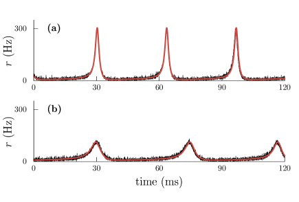
Figure 4: Electrical coupling promotes collective synchrony. The inclusion of inhibitory coupling degrades synchrony and slows down oscillations. The figure shows the time series of the mean firing rate $r$ of a network of $N=10^{4}$ QIF neurons with dynamics (1) (black) and of the FRE (5) (red). Panel (a) shows collective oscillations (frequency $f\approx 30.1$ Hz) of a network with gap junctions only ($J=0$). Panel (b) corresponds to a network with both gap junctions and inhibitory chemical coupling ($J=-\pi$), which both slows down ($f\approx 23.6$ Hz) and reduces the amplitude of collective oscillations. Parameters: $g=3$, $\bar{\eta}=1$, $\tau=10$ ms and $\Delta=1$.

To confirm the presence of collective oscillations in the original network of electrically coupled QIF neurons with dynamics Eq. (1), we carried out numerical simulations and compared them with those of the FRE (5). Fig. 4 shows the time series of the firing rate in the full and in the reduced system, which display a very good agreement. In panel (a) we considered a network with electrical coupling only. The frequency of the oscillations, $f\approx 30.1$ Hz, is close to the theoretical value at criticality, given by Eq. (8): $f_{\text{\scriptsize{H}}}=100/\pi\approx 31.8$ Hz. Therefore, in absence of chemical coupling and near the Hopf bifurcation, the frequency of the oscillations is almost independent of the coupling strength $g$ and closely follows Eq. (8). To further test the validity of Eq. (8) far from criticality, we numerically evaluated the frequency of the limit cycle of the FRE (5) (black solid line, Fig. 5) as the the coupling strength $g$ is increased from the Hopf bifurcation (at $g_{H}\approx 1.8$). The black dotted line corresponds to the Hopf frequency Eq. (8). We find that the frequency of the limit cycle remains close to this for a broad range of $g$ values.

Hopf instability in networks of electrically coupled QIF neurons occurs like the transition to synchronization in the Kuramoto model of coupled phase oscillators Kuramoto (1975). Considering $J=0$, we find the main features of the Kuramoto transition to collective synchronization: ($i$) In the limit of weak electrical coupling $g$, the Hopf boundary Eq. (7) can be written as

$$g_{H}\approx\frac{2\Delta}{\sqrt{\bar{\eta}}}.$$ (9)

For $\bar{\eta}=1$, Eq. (9) coincides with Kuramoto’s critical coupling for synchrony. ($ii$) As previously discussed, macroscopic oscillations emerge with a frequency determined by the most likely value of the natural frequencies in the network, see Eq. (3). For the case of the Lorentzian distribution of currents, Eq. (4), the most likely value of the frequency is

$$\bar{f}=\frac{\sqrt{\bar{\eta}}}{\pi\tau}.$$ (10)

($iii$) The Hopf bifurcation is always supercritical; cf. Appendix D. Taken together, for $\bar{\eta}>0$ and given a certain level of heterogeneity $\Delta$, synchronization occurs —at a critical coupling approximately given by Eq. (9)— with the nucleation of a small cluster of oscillators with natural frequencies Eq. (3) near $\bar{f}$. As electrical coupling $g$ is further increased, more and more oscillators become entrained to the frequency $\bar{f}$, resulting in a continuous and monotonous increase in the amplitude of the oscillations. This transition is in contrast to that of networks with inhibitory coupling and synaptic kinetics and/or delays, where synchrony is only achieved for weak heterogeneity and weak coupling, see, e.g., Devalle et al. (2017, 2018).

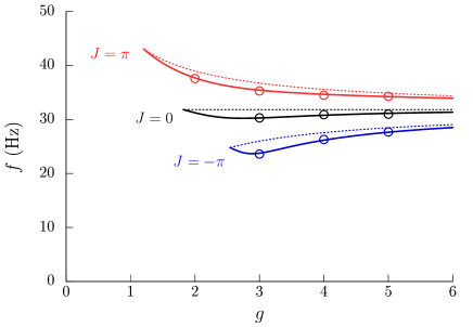
Figure 5: In the absence of chemical coupling (black), electrical coupling $g$ has little effect on the frequency of the oscillations Excitatory (red)/Inhibitory (blue) coupling speeds-up/slows-down collective oscillations. These effects tend to disappear for strong electrical coupling. The figure shows the frequency of the oscillations $f$ as a function of the strength of electrical coupling $g$ in networks with Excitation, $J=\pi$, Inhibition, $J=-\pi$, and without chemical coupling, $J=0$. Symbols ($\circ$) are frequencies obtained from numerical simulations of a network of $N=10^{4}$ QIF neurons Eqs. (1). Solid lines are numerically obtained frequencies from the FRE (5). Dotted lines correspond to the Hopf frequency given by Eq. (8). Parameters: $\bar{\eta}=1$, $\tau=10~{}$ms, and $\Delta=1$.

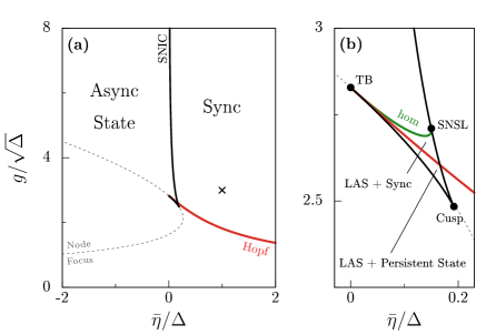
Figure 6: The phase diagram of the FRE (5) for electrical coupling only ($J=0$) is characterized by the presence of three codimension-2 bifurcation points (Takens-Bogdanov, TB; Saddle-Node Separatix Loop, SNSL; Cusp), all located at $\bar{\eta}\geq 0$. The region of synchronization (Sync) is limited by supercritical Hopf (red), SNIC (black), and homoclinic (green) bifurcations. Dashed line: Focus-Node boundary of the Asynchronous State. Panel (b) Enlargement of the region near the three codimension-2 points. There are two small regions of bistability between Asynchronous, low-activity-states (LAS) and Asynchronous Persistent States, and between LAS and Sync. Two Saddle-Node (SN) bifurcations are created at a Cusp point, at $(1/(3\sqrt{3}),4\sqrt{2}/3^{3/4})\approx(0.192,2.482)$. The upper SN line meets the homoclinic (hom) bifurcation in a SNSL point. At this point the upper SN becomes a SNIC bifurcation. The other SN bifurcation tangentially meets the homoclinic and the Hopf lines at a TB point, at $(0,2\sqrt{2})\approx(0,2.828)$. The Hopf boundary corresponds to Eq. (7). SN/SNIC and Focus/Node boundaries are obtained in parametric and explicit form, respectively, in Appendix C. The homoclinic boundary has been obtained numerically. The symbol $\times$ indicates the parameter value considered in Fig. 4(a).

The phase diagram depicted in Fig. 6 characterizes the dynamics of the firing rate model Eq. (5) with only electrical coupling. The red curve corresponds to the Hopf bifurcation line given by Eq. (7). According to Eq. (8), the frequency of the collective oscillations approaches zero as $\bar{\eta}\to 0$. This indicates that the Hopf line ends in a Takens-Bogdanov (TB) bifurcation at $\bar{\eta}=0$, see Fig. 6(b). At this codimension-2 point, the Hopf boundary tangentially meets a SN bifurcation and a homoclinic bifurcation. The homoclinic line moves parallel to the Hopf line for a while, it makes a sharp backward turn and then tangentially joins onto the upper branch of the SN bifurcation curve (two branches of SN bifurcations are created at the Cusp point), at a saddle-node-separatrix-loop (SNSL) point. At this point the SN boundary becomes a SNIC boundary that, together with the Hopf and homoclinic lines, encloses the region of synchronization (Sync) featuring collective oscillations. Note that in Fig. 6(b) we encounter a very small region of bistability between a Low-Activity State (LAS, node) and a persistent state (focus). Electrical coupling destabilizes the persistent state almost immediately after the SN line, leading to another small region of bistability between LAS and a small amplitude limit cycle (Sync) —which disappears in the homoclinic bifurcation.

Finally, the SNIC curve asymptotically approaches $\bar{\eta}=0$ as $g/\sqrt{\Delta}\to\infty$ (as suggested by the $N=2$ analysis in Section II.1). In this limit, all neurons are strongly coupled ($g\to\infty$) and/or are nearly identical ($\Delta\to 0$) so that they behave as a single QIF neuron with input current $\bar{\eta}$ .

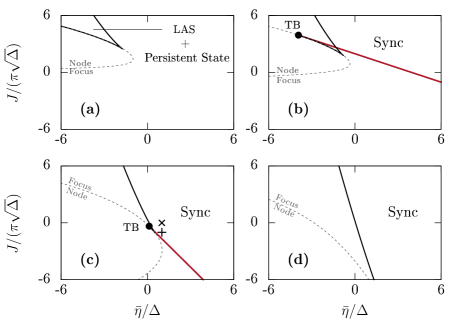
Figure 7: The phase diagram for networks with only chemical coupling, panel (a), is characterized by the presence of a Cusp bifurcation point. The inclusion of electrical coupling, panels (b-d), transforms the Cusp bifurcation scenario into that of Fig. 6, characterized by the presence of three codimension-2 bifurcation points. The panels show the phase diagrams of the FRE (5) with chemical coupling ($J>0$: Excitatory, $J<0$: Inhibitory) for (a) $g/\sqrt{\Delta}=0$, (b) $g/\sqrt{\Delta}=1$, (c) $g/\sqrt{\Delta}=3$, (d) $g/\sqrt{\Delta}=5$. The Hopf boundaries (red lines) are straight lines given by Eq. (7). SN/SNIC (black lines) and Focus/Node (dashed) boundaries are obtained in parametric form in Appendix C. Hopf and SN boundaries meet at a TB bifurcation point. To lighten the diagrams, Cusp, SNSL and homoclinic bifurcations are not shown. Symbols $\times$ and $+$ indicate the parameter values considered in Fig. 4.

IV.2 Networks with both chemical and electrical coupling

We finally analyze the dynamics of a population of QIF neurons with mixed, chemical and electrical synapses. Fig. 7(a) presents the possible dynamical regimes of a population with chemical synapses only, $g=0$. In contrast to networks with pure electrical coupling, where the bifurcation scenario is determined by the presence of three codimension-2 points, cf. Fig. 6, here there is only a Cusp point, see also Montbrió et al. (2015). This entails the presence of a persistent state (focus) coexisting with an asynchronous, LAS (node) within the cusp-shaped region in the top-left corner of Fig. 7(a). Additionally, the dashed line indicates that the asynchronous state is of focus type in a vast region of parameters for excitatory coupling, and always for inhibitory coupling.

Including electrical coupling, $g>0$, yields the Hopf bifurcation given by Eq. (7), which joins onto the lower branch of the SN bifurcation curve at a TB point, see Figs. 7(b,c). Hence, the bifurcation scenario for networks with electrical and chemical synapses matches that for networks with electrical synapses only: Similar to Fig. 6, the Hopf line cuts through the cusp-shaped region —the TB bifurcation demarcates the point where the Hopf boundary and the lower SN line intersect. Then, due to the presence of electrical coupling, the persistent state becomes only stable in a small parameter region confined between the Hopf and the lower SN line, see Fig. 7(b). As electrical coupling is increased, the TB point approaches the Cusp bifurcation, which results in an even smaller range of parameters for which the persistent state is stable. This agrees with numerical results using large networks of noisy, conductance-based and QIF neurons, and has been hypothesized to be a possible reason why electrical synapses are rarely found between excitatory neurons Ermentrout (2006).

Returning to the analysis of the FRE (5), we find for low values of $g$ that synchronization emerges predominantly for excitatory coupling, $J>0$, see Fig. 7(b). As electrical coupling is increased, the Sync region extends to the inhibitory region, $J<0$, and to larger values of $\bar{\eta}$ —note that in this coupling regime the emergence of collective oscillations mainly occurs via a SNIC bifurcation for excitation and via a Hopf bifurcation for inhibition, see Fig. 7(c). For even larger electrical coupling, the TB point moves further into the inhibitory region. That is, for strong electrical coupling the $J$-coordinate of the TB bifurcation rapidly decreases towards minus infinity whereas the other coordinate stays relatively close to the $\bar{\eta}=0$ axis . The SNIC bifurcation tilts towards a vertical line close to the $\bar{\eta}=0$ axis, because strong electrical coupling coerces all neurons to behave as a single QIF neuron with common input $\eta=\bar{\eta}$. Then, the SNIC bifurcation becomes the only transition between the two possible dynamical regimes, asynchrony or synchrony, see Fig. 7(d).

Fig. 4 shows how the addition of inhibitory coupling into a network with only electrical synapses degrades synchrony —parameters used in Fig. 4 correspond to the symbols shown in Fig. 7(c). The presence of inhibition clearly slows down the oscillations, as predicted by Eq. (8).

Although Eq. (8) is strictly valid only at the Hopf bifurcation, it is a good estimate of the frequency of the oscillations of the FRE (5). Fig. 5 depicts the comparison between Eq. (8) as a function of $g$ (dotted lines), with the actual frequencies numerically obtained using the FRE (5) (solid lines) and the QIF network Eq. (1) (symbols). In excitatory networks, the oscillations already emerge for weak values of $g$. In contrast, synchronizing inhibitory networks requires a much larger value of $g$, i.e. inhibition does not promote synchronization. Remarkably, only the presence of chemical coupling allows the frequency of the oscillations to deviate from $\bar{f}$, see Eqs. (8,10). Oscillations emerge with $f>\bar{f}$ for excitation and with $f<\bar{f}$ for inhibition, while they remain $f\approx\bar{f}$ for networks with only electrical coupling. As $g$ increases, the effects of chemical coupling are gradually washed out since an increasing number of neurons are entrained by electrical coupling to the most-likely frequency of the uncoupled network, $\bar{f}$. This dependence is well described by Eq. (8). Finally, since the level of heterogeneity $\Delta$ degrades synchrony, in Eq. (8) this term favors the deviation of the frequency from $\bar{f}$, and compensates for the homogenizing effect of electrical coupling. In the limit of identical neurons $\Delta\to 0$, the effects of instantaneous chemical coupling on the frequency vanish, since neurons synchronize in-phase and, at the instant of firing, all neurons become refractory.

V Conclusion and discussion

Firing rate models are very useful tools for investigating the dynamics of large networks of spiking neurons that interact via excitation and inhibition, see e.g. Wilson and Cowan (1972); Dayan and Abbott (2001); Ermentrout and Terman (2010); Hopfield (1984); Mongillo et al. (2008); Ben-Yishai et al. (1995); Hansel and Sompolinsky (1998); Tabak et al. (2000); Rankin et al. (2015); Martí and Rinzel (2013); Tsodyks M. (1998); Roxin et al. (2005); Roxin and Montbrió (2011). Remarkably, using a recently proposed approach to derive exact firing rate equations for networks of excitatory and/or inhibitory QIF neurons Montbrió et al. (2015); Luke et al. (2013), Laing has found that electrical synapses can also be incorporated in the framework of firing rate models Laing (2015). Yet, the FRE in Laing (2015) are not exact, and their mathematical form makes the analysis intractable.

Here we showed that the FRE corresponding to a network of QIF neurons with both chemical and electrical synapses can be exactly obtained, without the need for any approximation. Much in the spirit of firing rate models, the resulting FRE (5) are simple in form and highly amenable to analysis. Moreover, in Appendix B, we demonstrate that relaxing the approximation invoked in Laing (2015) the FRE derived by Laing simplify to our Eqs. (5).

At first glance, the mathematical form of Eqs. (5) already unveils two interesting features of electrical and chemical coupling, see also Eq. (6): ($i$) Chemical coupling tends to shift the center of the distribution of membrane potentials (given by $v$), while electrical coupling tends to reduce the width of the distribution (given by $r$), potentially promoting the emergence of synchronization; ($ii$) While in the original network of QIF neurons electrical coupling is mediated by membrane potential differences, at the mean-field level the electrical interaction is solely mediated by the mean firing rate $r$.

The mathematical analysis of the FRE (5) unravels how chemical and electrical coupling shape the dynamics of globally coupled populations of QIF neurons with Lorentzian heterogeneity. Some of our results were already reported in previous work, and confirm the value and the validity of the FRE (5). An important conclusion of our study is that the presence of electrical coupling, $g\neq 0$, generally implies the appearance of a supercritical Hopf bifurcation, see Eq. (7). This Hopf bifurcation meets a SN bifurcating line in a codimension-2 TB point, causing a drastic reduction of the region of bistability between low-activity and persistent asynchronous states, see Figs. 6 and 7. The Hopf bifurcation destabilizes the persistent state producing synchronous oscillations, which then are abolished via a homoclinic bifurcation. Previous studies of networks of excitatory and inhibitory neurons showed that synchrony often destroys persistent states Hansel and Mato (2001, 2003); Gutkin et al. (2001); Laing and Chow (2001); Kanamaru and Sekine (2003). Moreover, the generality of the bifurcation scenario of Figs. 6 and 7 —characterized by three codimension-2 points, TB, Cusp and SNSL—, is confirmed in previous studies analyzing closely related systems Sakaguchi et al. (1988); Zaks et al. (2003); M.Childs and Strogatz (2008); Lafuerza et al. (2010).

Networks of spiking neurons with strong excitatory coupling display robust persistent states. These states emerge at a Cusp bifurcation, see Fig. 7(a). Of particular relevance to our study is the work by Ermentrout Ermentrout (2006). He found that electrical coupling tends to synchronize neurons, and that this anihilates persistent states via the bifurcation scenario described in Figs. 6 and  7. Persistent activity may underlie important cognitive functions such as working memory, and has been suggested as a possible reason for the lack of electrical coupling between excitatory neurons Ermentrout (2006). According to Ermentrout (2006), ‘the main role for gap junctions is to encourage synchronization during rhythmic behavior. Synchrony, because it leads to a shared refractory period between neurons can lead to the extinction of persistent activity’.

The Hopf bifurcation is always supercritical. In Ostojic et al. (2009), Ostojic et al. analyzed the super- or sub-critical character of the Hopf bifurcation in networks of electrically coupled leaky integrate and fire (LIF) neurons. At variance with QIF neurons, LIF neurons do not have spikes and, hence, modeling electrical coupling requires an additional parameter Lewis and Rinzel (2003). This parameter enables one to adjust the shape of the spikelet elicited in the postsynaptic cell due to an action potential in the presynaptic cell. Ostojic et al. Ostojic et al. (2009) found that the Hopf bifurcation is supercritical when the spikelets are effectively excitatory, while inhibitory spikelets lead to subcritical Hopf bifurcations. For the QIF model, the spikelet elicited in a postsynaptic cell by the transmission of a presynaptic spike has a net excitatory effect —see Fig. 1(b)—, and hence our result that the Hopf bifurcation is supercritical is in agreement with the results in Ostojic et al. (2009). Yet, we note that our result also includes networks with chemical synapses, and not only networks with electrical synapses, as in Ostojic et al. (2009).

Another important result by Ostojic et al. Ostojic et al. (2009) is that electrical coupling can lead to oscillations even in the presence of strong heterogeneity. Our Eq. (7) is consistent with this. Kopell and Ermentrout Kopell and Ermentrout (2004) also investigated the robustness of synchrony against current heterogeneities in networks with both electrical and inhibitory synapses. They found that a small amount of electrical coupling, added to an already significant inhibitory coupling, can increase synchronization more than a very large increase in the inhibitory coupling. In Fig. 4 we show that increasing inhibition reduces the amplitude of the oscillations in a network with $g\neq 0$. In addition, Fig. 7 shows that, for a given value of $g$, increasing inhibition leads to asynchrony. This level of inhibition increases with electrical coupling, in line with the results in Kopell and Ermentrout (2004). Two studies Ostojic et al. (2009); Viriyopase et al. (2016) also investigated the frequency of the emerging oscillations in networks with electrical synapses. This frequency remains tied to the mean firing rate $f_{i}$ in the network (i.e. near $\bar{f}$), as our Eq. (8) suggests. In Fig. 5 we confirm that, in networks with only electrical synapses, the frequency of the oscillations remains near the most likely $f_{i}$-value: $\bar{f}$.

The result that the Hopf bifurcation is always supercritical, and that the frequency of the emerging oscillations is given by $\bar{f}$ evoke the paradigmatic synchronization transition in the Kuramoto model Kuramoto (1975). For weakly electrically-coupled networks, we find that the onset of oscillations occurs at the Kuramoto’s critical coupling for synchrony, Eq. (9). When considering chemical coupling, the frequency of the oscillations deviates from $\bar{f}$, increasing/decreasing for excitatory/inhibitory coupling. The intensity of this deviation depends on the ratio of chemical to electrical coupling, as Eq. (8) suggests. Fig. 5 confirms that strong electrical coupling overcomes the effect of excitation/inhibition onto the frequency of the oscillations, approximately as dictated by Eq. (8).

Together with the firing rate model derived in Laing (2015), the FRE (5) constitute a unique example of a firing rate model with both electrical and chemical coupling. The numerical simulations of the original QIF network Eq. (1) are in agreement with the FRE (5) —see Figs. 4, 5—, underlining the validity of the reduction method applied. Interestingly, the fixed points of the FRE (5) with chemical synapses ($g=0$, $J\neq 0$) can be cast in the form of a traditional firing rate model

$$r_{*}=\Phi(\bar{\eta}+J\tau r_{*}),$$ (11)

where $\Phi(x)=\sqrt{x+\sqrt{x^{2}+\Delta^{2}}}/(\sqrt{2}\pi\tau)$ is the so-called transfer function of the heterogeneous QIF network  Esnaola-Acebes et al. (2017); Devalle et al. (2017, 2018). The FRE (5) with electrical synapses ($g\neq 0$), however, cannot be written in the form of Eq. (11). Therefore, the link pointed by Eq. (11) between traditional firing rate models and Eqs. (5) is lost when electrical coupling is considered.

Appendix A: Derivation of the Firing Rate Equations

In the thermodynamic limit, $N\to\infty$, we drop the indices for the individual neuronal dynamics Eq. (1), and denote $\rho(V|\eta,t)dV$ as the fraction of neurons with membrane potentials between $V$ and $V+dV$, and parameter $\eta$ at time $t$. Accordingly, the parameter $\eta$ becomes a continuous random variable that is distributed according to a probability distribution function, which here is considered to be a Lorentzian $L_{\Delta,\bar{\eta}}(\eta)$ of half-width $\Delta$ and centered at $\bar{\eta}$, see Eq. (4). The conservation of the number of neurons leads to the continuity equation

$$\tau\partial_{t}\rho+\partial_{V}\left[(V^{2}+\eta+g(v-V)+J\tau r)\rho\right]=0,$$ (A1)

where we explicitly included the velocity given by the continuous equivalent of Eq. (1). We also defined the mean value of the membrane potential as

$$v(t)=\int_{-\infty}^{\infty}\int_{-\infty}^{\infty}\rho(V|\eta,t)~{}VL_{\Delta,\bar{\eta}}(\eta)~{}dVd\eta.$$ (A2)

Next, we consider the family of conditional density functions Montbrió et al. (2015)

$$\rho(V|\eta,t)=\frac{1}{\pi}\frac{x(\eta,t)}{\left[V-y(\eta,t)\right]^{2}+x(\eta,t)^{2}},$$ (A3)

which are Lorentzian functions with time-dependent half-width $x(\eta,t)$, centered at $y(\eta,t)$. Substituting (A3) into the continuity equation (A1), we find that, for each value of $\eta$, variables $x$ and $y$ must obey two coupled equations,

$$\tau\dot{x}(\eta,t) = 2x(\eta,t)y(\eta,t)-gx(\eta,t),$$ (A4a)

$$\tau\dot{y}(\eta,t) = \eta-x(\eta,t)^{2}+y(\eta,t)^{2}$$

$$\hskip 24.18501pt-g\big{[}y(\eta,t)-v\big{]}+J\tau r,$$

that can be written in complex form as

$$\tau\partial_{t}w(\eta,t)=i\big{[}\eta-w(\eta,t)^{2}+J\tau r\big{]}+g\big{[}iv-w(\eta,t)\big{]}$$ (A5)

where $w(\eta,t)\equiv x(\eta,t)+iy(\eta,t)$. For a particular value of $\eta$, the firing rate $r$ of the population of QIF neurons is related to the width $x$ of the Lorentzian ansatz (A3). Specifically, the firing rate $r(\eta,t)$ for each $\eta$ value at time $t$ is the probability flux at infinity: $r(\eta,t)=\rho(V\to\infty|\eta,t)\dot{V}(V\to\infty|\eta,t)$, which yields the identity

$$x(\eta,t)=\pi\tau r(\eta,t).$$ (A6)

Hence, integrating this quantity over the distributions of currents Eq. (4) provides the mean firing rate

$$r(t)=\frac{1}{\tau\pi}\int_{-\infty}^{\infty}x(\eta,t)L_{\Delta,\bar{\eta}}(\eta)d\eta.$$ (A7)

Likewise, we can link the center $y(\eta,t)$ of the Lorentzian ansatz Eq. (A3) with the mean of the (conditional) membrane potential via

$$y(\eta,t)=\text{p.v.}\int_{-\infty}^{\infty}\rho(V|\eta,t)VdV.$$ (A8)

Note that the Lorentzian distribution does not have finite moments so that the integral in Eq. (A8) needs to be taken as the Cauchy principal value (i.e. $\text{p.v.}\int_{-\infty}^{\infty}\rho VdV=\lim_{R\to\infty}\int_{-R}^{R}\rho VdV$). Then, Eq. (A2) becomes

$$v(t)=\int_{-\infty}^{\infty}y(\eta,t)L_{\Delta,\bar{\eta}}(\eta)d\eta.$$ (A9)

The integrals in (A7,A9) can be evaluated closing the integral contour in the complex $\eta$-plane and using Cauchy’s residue theorem. The integrals must however be performed carefully, so that the variable $x(\eta,t)$ remains non-negative. To make the analytic continuation of $w(\eta,t)$ from real to complex-valued $\eta$, we define $\eta\equiv\eta_{r}+i\eta_{i}$. This continuation is possible into the lower half-plane $\eta_{i}<0$, since this guarantees the half-width $x(\eta,t)$ to remain non-negative: $\partial_{t}x(\eta,t)=-\eta_{i}>0$, at $x=0$. Therefore, we perform contour integration in Eq. (A7) and Eq. (A9) along the arc $|\eta|e^{i\vartheta}$ with $|\eta|\to\infty$ and $\vartheta\in(-\pi,0)$. This contour encloses one pole of the Lorentzian distribution Eq. (4). Then, we find that the firing rate and the mean membrane potential depend only on the value of $w$ at the pole of $L_{\Delta,\bar{\eta}}(\eta)$ in the lower half $\eta$-plane:

$$\pi\tau r(t)+iv(t)=w(\bar{\eta}-i\Delta,t),$$

As a result, we only need to evaluate Eq. (A5) at $\eta=\bar{\eta}-i\Delta$, and obtain a system of FRE composed of two ordinary differential equations as given in Eq. (5),

$$\tau\dot{r} = \frac{\Delta}{\tau\pi}+2rv-gr,$$

$$\tau\dot{v} = v^{2}+\bar{\eta}-(\pi\tau r)^{2}+J\tau r,$$

in terms of the population-mean firing rate $r$ and the population-mean membrane potential $v$. Multiplying the Lorentzian ansatz Eq. (A3) by $L_{\Delta,\bar{\eta}}(\eta)$ and integrating over $\eta$, we finally obtain the total density of neurons Eq. (6) as

$$\rho(V,t)=\frac{1}{\pi}\frac{\pi\tau r(t)}{[V-v(t)]^{2}+\pi^{2}\tau^{2}r(t)^{2}},$$

where we again applied Cauchy’s residue theorem by using that the ansatz Eq. (A3) is analytic in the lower $\eta$-complex plane. Hence, the total density of the population of QIF neurons is a Lorentzian distribution centered at $v(t)$ and half-width $\pi\tau r(t)$, which evolves according to the FRE (5).

Appendix B: Connection between the FRE in Laing (2015) and Eq. (5)

The derivation of the FRE (5) is exact in the thermodynamic limit, and does not rely on any approximation. Here we show that the Eqs. (2.35&2.36) in Laing (2015) reduce to our Eq. (5) after adopting a limit in which the derivation performed in Laing (2015) becomes exact.

In contrast to our Eq. (5b), note that Eq. (2.36) in Laing (2015) contains a diffusive term,

$$g[Q(t)-v(t)],$$ (B1)

where the function $Q(t)$ is defined as

$$Q(t)=\frac{i}{2}\sum_{m=1}^{\infty}\frac{\rho^{m+1}-\rho^{m-1}}{\rho+1+\epsilon}\left[z^{m}-\bar{z}^{m}\right]$$ (B2)

with $0<\epsilon\ll 1$, and $\rho=\sqrt{2\epsilon+\epsilon^{2}}-1-\epsilon$. The variable $z$ in Eq. (B2) is the complex Kuramoto order parameter (the bar denotes complex conjugation), which is related to the variables $r$ and $v$ in the FRE (5) via the change of variables Montbrió et al. (2015)

$$\pi r+iv=\frac{1-\bar{z}}{1+\bar{z}}.$$ (B3)

The parameter $\epsilon$, defined in Eq. (2.7) in Laing (2015), was used to approximate the mean voltage $v$, see also Ermentrout (2006). In the limit $\epsilon\to 0$ this approximation becomes exact, but this limit was not considered in Laing (2015). In consequence, to use the Eqs. (2.35&2.36) in Laing (2015), the infinite series Eq. (B2) was truncated after 100 terms, and the bifurcation analysis of the mean-field model could only be performed numerically.

Using the geometric series formula ($|z|<1$) and the transformation of variables Eq. (B3), we find

$$\lim_{\epsilon\to 0}Q(t)=i\sum_{m=1}^{\infty}(-1)^{m}\left[z^{m}-\bar{z}^{m}\right]=\frac{2\text{Im}(z)}{(1+z)(1+\bar{z})}=v.$$

Hence we have showed that the diffusive term Eq. (B1) identically vanishes when the mean-field reduction becomes exact (i.e. in the limit $\epsilon\to 0$), and the FRE in Laing (2015) reduce to Eqs. (5).

Appendix C: Bifurcation analysis of the Firing Rate Equations

The FRE (5) have five free parameters. The number of effective parameters can be reduced to three through non-dimensionalization, defining

$$\tilde{\eta}=\bar{\eta}/\Delta,~{}\tilde{g}=g/\sqrt{\Delta},~{}\tilde{J}=J/(\pi\sqrt{\Delta}),$$

and rescaling variables as

$$\tilde{r}=\tau\pi r/\sqrt{\Delta},~{}\tilde{v}=v/\sqrt{\Delta},~{}\tilde{t}=\sqrt{\Delta}t/\tau.$$

Then, the firing rate model becomes

$$\frac{d\tilde{r}}{d\tilde{t}} = 1+2\tilde{r}\tilde{v}-\tilde{g}\tilde{r},$$ (C1a)

$$\frac{d\tilde{v}}{d\tilde{t}} = \tilde{v}^{2}+\tilde{\eta}-\tilde{r}^{2}+\tilde{J}\tilde{r},$$ (C1b)

The fixed points $(\tilde{r}_{*},\tilde{v}_{*})$ of Eq. (C1) satisfy

$$\tilde{v}_{*}=\frac{\tilde{g}}{2}-\frac{1}{2\tilde{r}_{*}}.$$ (C2)

Linearization about the fixed points Eq. (C2) gives the eigenvalues

$$\lambda_{\pm}=\frac{1}{2}\left(4\tilde{v}_{*}-\tilde{g}\pm\sqrt{\tilde{g}^{2}+8\tilde{r}_{*}(\tilde{J}-2\tilde{r}_{*})}\right).$$ (C3)

For networks with only chemical synapses (i.e. $g=0$), the real part of the eigenvalues remains always negative (since $v_{*}<0$), and a Hopf bifurcation is not possible. However, chemical coupling has a direct influence on the real part of the eigenvalues Eq. (C3), and may produce oscillatory instabilities if the argument of the square root is a real number.

V.1 Hopf boundaries and Takens-Bogdanov point

The Hopf boundaries can be obtained when imposing Re($\lambda_{\pm})=0$ in Eq. (C3), which gives $\tilde{g}=4\tilde{v}_{*}$. Then, using Eq. (C2), we find

$$\tilde{g}_{H}=2/\tilde{r}_{*}.$$ (C4)

Substituting Eq. (C4) in the $v$-fixed point equation Eq. (C1b), and solving for $\tilde{\eta}$, we obtain

$$\tilde{\eta}_{H}=r_{*}^{2}-\tilde{J}\tilde{r}_{*}-\frac{1}{4\tilde{r}_{*}^{2}}.$$ (C5)

Solving Eq. (C4) for $\tilde{r}_{*}$ and substituting it into Eq. (C5) we obtain the Hopf boundaries in explicit form

$$\tilde{\eta}_{H}=-\frac{2\tilde{J}}{\tilde{g}}+\frac{4}{\tilde{g}^{2}}-\frac{\tilde{g}^{2}}{16}.$$ (C6)

The frequency of the oscillations is given by the imaginary part of the eigenvalues Eq. (C3) at criticality that, using the fixed points of Eqs. (C1) and Eq. (C4), reduces to the explicit formula

$$\tilde{f}_{H}=\frac{1}{\pi}\sqrt{\tilde{\eta}+\frac{\tilde{J}}{\tilde{g}}}.$$ (C7)

The frequency becomes zero at a Takens-Bogdanov (TB) point, when $\tilde{\eta}=-\tilde{J}/\tilde{g}$. Inserting this condition into Eq. (C6) we obtain the coordinates of the TB point

$$\left(\tilde{\eta},\tilde{J}\right)_{\text{\scriptsize{TB}}}=\left(\frac{\tilde{g}^{2}}{16}-\frac{4}{\tilde{g}^{2}},\frac{4}{\tilde{g}}-\frac{\tilde{g}^{3}}{16}\right),$$ (C8)

see also Fig. 7. For $\tilde{J}=0$, the TB point is located at

$$\left(\tilde{\eta},\tilde{g}\right)_{\text{\scriptsize{TB}}}=\left(0,2\sqrt{2}\right)$$ (C9)

in the phase diagram Fig. 6.

V.2 Saddle-node boundaries

The boundaries of the saddle-node bifurcations are obtained by setting $\lambda_{\pm}=0$ in Eq. (C3), using Eq. (C2), and solving for $\tilde{g}$:

$$\tilde{g}_{sn}=\frac{1}{\tilde{r}_{*}}-2\tilde{J}\tilde{r}_{*}^{2}+4\tilde{r}_{*}^{3}\ .$$ (C10)

Substituting (C10) in the $v$-fixed point Eq. (C1b), and solving for $\tilde{\eta}$, we obtain

$$\tilde{\eta}_{sn}=\tilde{r}_{*}^{2}-4\tilde{r}^{6}_{*}+\tilde{J}\tilde{r}_{*}\left(4\tilde{r}_{*}^{4}-J\tilde{r}_{*}^{3}-1\right).$$ (C11)

The saddle node boundaries are plotted in the $(\tilde{\eta},\tilde{g})$ phase diagram in Fig. 6. The same boundaries can be represented in the $(\tilde{\eta},\tilde{J})$ phase diagram when solving Eq. (C10) for $\tilde{J}$

$$\tilde{J}_{sn}=\frac{1}{2\tilde{r}_{*}^{3}}-\frac{\tilde{g}}{2\tilde{r}_{*}^{2}}+2\tilde{r}_{*}$$ (C12)

and replacing $\tilde{J}$ by Eq. (C12) in Eq. (C11) gives

$$\tilde{\eta}_{sn}=\frac{\tilde{g}}{\tilde{r}_{*}}-\frac{\tilde{g}^{2}}{4}-\frac{3}{4\tilde{r}_{*}^{2}}-r_{*}^{2}.$$

These saddle-node boundaries are shown in black for different values of $\tilde{g}$ in Fig. 7.

V.3 Focus-Node boundaries

The boundaries in the phase diagram Fig. 7 in which the stable asynchronous state changes from Focus to Node can be obtained in parametric form equating the square root in Eq. (C3) to zero. This gives

$$\tilde{J}_{FN}=\frac{16\tilde{r}_{*}^{2}-\tilde{g}^{2}}{8\tilde{r}_{*}}.$$

Substituting $\tilde{J}_{FN}$ into the $v$-fixed point Eq. (C1b), and using Eq. (C2) we find

$$\tilde{\eta}_{FN}=\frac{1}{8\tilde{r}_{*}^{2}}\left(-2+4\tilde{g}\tilde{r}_{*}-\tilde{g}^{2}\tilde{r}_{*}^{2}-8\tilde{r}_{*}^{4}\right).$$

For networks without chemical coupling, $\tilde{J}=0$, the Focus-Node boundary can be obtained in explicit form

$$\tilde{\eta}_{FN}=2-\frac{4}{\tilde{g}^{2}}-\frac{3\tilde{g}^{2}}{16}.$$

This is the dashed boundary depicted in Fig. 6.

Appendix D: Small-amplitude equation near the Hopf bifurcation

In this Appendix we derive the small amplitude equation near the Hopf bifurcation, and show that the Hopf bifurcation is always supercritical. The derivation is performed using multiple-scales analysis, see e.g. Kuramoto (1984). We first expand the solution

$$\binom{\tilde{r}}{\tilde{v}}=\binom{r_{0}}{v_{0}}+\epsilon\binom{r_{1}}{v_{1}}+\epsilon^{2}\binom{r_{2}}{v_{2}}+\dots$$ (D1)

in powers of a small parameter $\epsilon\ll 1$, about a fixed point $(r_{0},v_{0})$ of Eqs. (C1) at the Hopf bifurcation. In addition, we introduce the deviation from the Hopf bifurcation Eq. (C6) of parameter $\tilde{\eta}$ as

$$\tilde{\eta}-\tilde{\eta}_{H}=\chi\epsilon^{2},$$ (D2)

where $\chi$ determines the sign of the deviation. Finally, we define the slow time

$$T=\epsilon^{2}t.$$ (D3)

Then, the time differentiation is transformed as

$$\frac{d}{dt}\to\partial_{t}+\epsilon^{2}\partial_{T}.$$ (D4)

Plugging Eqs. (D1,D2,D4) into Eq. (C1) gives

$$\left[\partial_{t}+\epsilon^{2}\partial_{T}-L_{0}\right]\left[\epsilon\binom{r_{1}}{v_{1}}+\epsilon^{2}\binom{r_{2}}{v_{2}}+\dots\right]-\epsilon^{2}\binom{0}{\chi}=$$

$$\hskip 113.81102pt=\epsilon^{2}N_{2}+\epsilon^{3}N_{3}+\dots,$$ (D5)

where

$$L_{0}=\begin{pmatrix}2v_{0}-\tilde{g}&2r_{0}\\ \tilde{J}-2r_{0}&2v_{0}\end{pmatrix}.$$ (D6)

and

$$N_{2}=\binom{2r_{1}v_{1}}{v_{1}^{2}-r_{1}^{2}},\quad N_{3}=\binom{2r_{1}v_{2}+2r_{2}v_{1}}{2v_{1}v_{2}-2r_{1}r_{2}}.$$ (D7)

Critical eigenvectors

Using Eqs. (C3,C4), we define the critical frequency as

$$\omega_{0}=\frac{1}{2\tilde{g}}\sqrt{64-\tilde{g}^{4}-16\tilde{J}\tilde{g}},$$ (D8)

so that the matrix Eq. (D6) can be written as

$$L_{0}=\begin{pmatrix}-\tilde{g}/2&4/\tilde{g}\\ -\tilde{g}/16(\tilde{g}^{2}+4\omega_{0}^{2})&\tilde{g}/2\end{pmatrix}.$$ (D9)

The right-eigenvector of Eq. (D9) is

$$\mathbf{u}_{R}=\binom{4/\tilde{g}}{\tilde{g}/2+i\omega_{0}}.$$ (D10)

Imposing the condition $\mathbf{u}_{L}\mathbf{u}_{R}=1$, the left-eigenvector of $L_{0}$ is

$$\mathbf{u}_{L}=\frac{1}{2\omega_{0}}\left(\frac{2\tilde{g}\omega_{0}+i\tilde{g}^{2}}{8},-i\right).$$ (D11)

Analysis of multiple scales

At order $\epsilon$, Eq. (D5) is

$$\binom{\dot{r}_{1}}{\dot{v}_{1}}-L_{0}\binom{r_{1}}{v_{1}}=\binom{0}{0}.$$ (D12)

This system of differential equations has a general solution

$$\binom{r_{1}}{v_{1}}=Ae^{i\omega_{0}\tilde{t}}\mathbf{u}_{R}+\text{c.c},$$ (D13)

which is the so-called neutral solution.

At order $\epsilon^{2}$, Eq. (D5) is

$$\binom{\dot{r}_{2}}{\dot{v}_{2}}-L_{0}\binom{r_{2}}{v_{2}}-\binom{0}{\chi}=N_{2}.$$ (D14)

Substituting the neutral solution Eq. (D13) into Eq. (D7) we find

$$N_{2} = \binom{8}{(\tilde{g}^{4}+4\tilde{g}^{2}\omega_{0}^{2}-64)/(2\tilde{g}^{2})}|A|^{2}$$

$$+ \binom{4+8i\omega_{0}/\tilde{g}}{\tilde{g}^{2}/4+i\tilde{g}\omega_{0}-\omega_{0}^{2}-16/\tilde{g}^{2}}A^{2}e^{2i\omega_{0}\tilde{t}}$$

$$+$$ c.c.

Next we use the following ansatz

$$\binom{r_{2}}{v_{2}}=\binom{r_{20}}{v_{20}}+\binom{r_{22}}{v_{22}}e^{2i\omega_{0}\tilde{t}}+\text{c.c.}$$ (D15)

and substitute it into Eq. (D14). We find

$$r_{20} = \frac{2}{\tilde{g}^{3}\omega_{0}^{2}}\left[2\tilde{g}^{2}\chi-(64+\tilde{g}^{4}-4\tilde{g}^{2}\omega_{0}^{2})|A|^{2}\right],$$

$$v_{20} = \frac{1}{4\tilde{g}\omega_{0}^{2}}\left[2\tilde{g}^{2}\chi-(64+\tilde{g}^{4}+4\tilde{g}^{2}\omega_{0}^{2})|A|^{2}\right],$$

$$r_{22} = \frac{A^{2}}{3\tilde{g}^{3}\omega_{0}^{2}}\left[64+\tilde{g}^{2}(\tilde{g}+2i\omega_{0})(\tilde{g}-10i\omega_{0})\right],$$

$$v_{22} = \frac{A^{2}}{24\tilde{g}^{2}\omega_{0}^{2}}\left[\tilde{g}(64+\tilde{g}(\tilde{g}+2i\omega_{0})^{2}(\tilde{g}-8i\omega_{0}))+256i\omega_{0}\right].$$

Substituting Eqs. (D13,D15) into the cubic term $N_{3}$ in Eq. (D7), we find

$$N_{3}=\binom{(\tilde{g}+2i\omega_{0})Ar_{20}+\tfrac{8}{\tilde{g}}(Av_{20}+A^{*}v_{22})+(\tilde{g}-2i\omega_{0})A^{*}r_{22}}{(\tilde{g}+2i\omega_{0})Av_{20}-\tfrac{8}{\tilde{g}}(Ar_{20}+A^{*}r_{22})+(\tilde{g}-2i\omega_{0})A^{*}v_{22}}e^{i\omega_{0}\tilde{t}}+\text{c.c.}+\binom{\tfrac{8}{\tilde{g}}v_{22}+(\tilde{g}+2i\omega_{0})r_{22}}{-\tfrac{8}{\tilde{g}}r_{22}+(\tilde{g}+2i\omega_{0})v_{22}}Ae^{3i\omega_{0}\tilde{t}}+\text{c.c.}$$ (D16)

The solvability condition at order $\epsilon^{3}$ is

$$\int_{0}^{2\pi/\omega_{0}}\mathbf{u}_{L}\left[\partial_{T}\binom{r_{1}}{v_{1}}-N_{3}\right]e^{-i\omega_{0}\tilde{t}}~{}d\tilde{t}=0.$$ (D17)

Substituting Eqs. (D11,D13,D16) into Eq. (D17), we find the amplitude equation

$$\partial_{T}A=(a+ib)\chi A-(c+id)A|A|^{2},$$ (D18)

with the coefficients

$$a = \frac{4\tilde{g}^{3}}{64-\tilde{g}^{4}-16\tilde{g}\tilde{J}},$$

$$b = \frac{32\tilde{g}(8-\tilde{g}\tilde{J})}{(64-\tilde{g}^{4}-16\tilde{g}J)^{3/2}},$$

$$c = \frac{16\tilde{g}(8-\tilde{g}\tilde{J})}{64-\tilde{g}^{4}-16\tilde{g}J},$$

$$d = \frac{16}{3}~{}\frac{3(64-\tilde{g}^{4})\tilde{J}-8\tilde{g}\tilde{J}+40\tilde{g}^{3}}{(64-\tilde{g}^{4}-16\tilde{g}J)^{3/2}},$$

where we used Eq. (D8) to express $a-d$ in terms of $\tilde{J}$ and $\tilde{g}$. Defining the amplitude $R$ and the phase $\Psi$ via

$$A=Re^{i\psi},$$

one may alternatively write Eq. (D18) as

$$R^{\prime} = \chi aR-cR^{3},$$

$$\psi^{\prime} = \chi b-dR^{2}.$$

where primes refer to differentiation with respect to $T$. An oscillatory solution with amplitude $R=R_{s}$ and phase $\psi=\omega T+\psi_{0}$, with

$$R_{s}=\sqrt{\frac{a}{|c|}},\quad\omega=\chi b-dR_{s}^{2},$$

appears in the supercritical ($\chi>0$) region for $c>0$, and in the subcritical region for $c<0$.

Remarkably, the coefficient $c$ is always positive and hence the Hopf bifurcation is always supercritical. This can be seen as follows: First, note that the denominator of $c$ remains always positive along the Hopf boundary Eq. (C6), and becomes zero at the Takens-Bogdanov point Eq. (C8). Second, note that the numerator of $c$ is positive for $\tilde{J}=0$ and may potentially change sign at $\tilde{J}_{c}=8/\tilde{g}$. However, this change of sign always occurs after the TB point ($\tilde{J}_{c}>\tilde{J}_{\text{{\scriptsize{TB}}}}$) in which the Hopf bifurcation ends, see Eq. (C8).

Finally, the approximate solution in terms of the original variables reads

$$\binom{r}{v}\approx\binom{r_{0}}{v_{0}}+\epsilon\binom{r_{1}}{v_{1}}=\binom{r_{0}}{v_{0}}+\epsilon R_{s}\mathbf{u}_{R}e^{i(\omega_{0}+\epsilon^{2}\omega)\tilde{t}}+\text{c.c.},$$

which describes an oscillatory motion in the critical eigenplane, with a small amplitude firing rate (for $\tilde{\eta}\geq\tilde{\eta}_{H}$)

$$r_{A}=\epsilon R_{s}\frac{g}{4}=2\sqrt{\frac{\tilde{\eta}-\tilde{\eta}_{H}}{8-\tilde{g}\tilde{J}}}.$$ (D19)

References

- Wang (2010) X.-J. Wang, Physiological Reviews 90, 1195 (2010).
- Nagy et al. (2018) J. I. Nagy, A. E. Pereda, and J. E. Rash, Biochimica et Biophysica Acta (BBA) - Biomembranes 1860, 102 (2018).
- Connors (2017) B. W. Connors, Developmental Neurobiology 77, 610 (2017).
- Traub et al. (2018) R. D. Traub, M. A. Whittington, R. Gutiérrez, and A. Draguhn, Cell and Tissue Research 373, 671 (2018).
- Bennett and Zukin (2004) M. V. Bennett and R. Zukin, Neuron 41, 495 (2004).
- Connors and Long (2004) B. W. Connors and M. A. Long, Annual Review of Neuroscience 27, 393 (2004).
- Whittington et al. (2000) M. Whittington, R. Traub, N. Kopell, B. Ermentrout, and E. Buhl, Int. Journal of Psychophysiol. 38, 315 (2000), ISSN 0167-8760.
- Kopell and Ermentrout (2004) N. Kopell and B. Ermentrout, Proceedings of the National Academy of Sciences 101, 15482 (2004).
- Pfeuty et al. (2007) B. Pfeuty, D. Golomb, G. Mato, and D. Hansel, Frontiers in Computational Neuroscience 1, 8 (2007), ISSN 1662-5188.
- Ermentrout (2006) B. Ermentrout, Phys. Rev. E 74, 031918 (2006).
- Viriyopase et al. (2016) A. Viriyopase, R.-M. Memmesheimer, and S. Gielen, Journal of Neurophysiology 116, 232 (2016).
- Holzbecher and Kempter (2018) A. Holzbecher and R. Kempter, European Journal of Neuroscience 48, 3446 (2018).
- Guo et al. (2012) D. Guo, Q. Wang, and M. c. v. Perc, Phys. Rev. E 85, 061905 (2012).
- Tchumatchenko and Clopath (2014) T. Tchumatchenko and C. Clopath, Nature Communications 5, 5512 (2014).
- Lewis and Rinzel (2003) T. J. Lewis and J. Rinzel, Journal of Computational Neuroscience 14, 283 (2003).
- Chow and Kopell (2000) C. C. Chow and N. Kopell, Neural Computation 12, 1643 (2000).
- Ostojic et al. (2009) S. Ostojic, N. Brunel, and V. Hakim, Journal of Computational Neuroscience 26, 369 (2009), ISSN 1573-6873.
- Pfeuty et al. (2003) B. Pfeuty, G. Mato, D. Golomb, and D. Hansel, Journal of Neuroscience 23, 6280 (2003).
- Coombes (2008) S. Coombes, SIAM Journal on Applied Dynamical Systems 7, 1101 (2008).
- Mancilla et al. (2007) J. G. Mancilla, T. J. Lewis, D. J. Pinto, J. Rinzel, and B. W. Connors, Journal of Neuroscience 27, 2058 (2007).
- Wilson and Cowan (1972) H. R. Wilson and J. D. Cowan, Biophys. J. 12, 1 (1972).
- Dayan and Abbott (2001) P. Dayan and L. F. Abbott, Theoretical neuroscience (Cambridge, MA: MIT Press, 2001).
- Ermentrout and Terman (2010) G. B. Ermentrout and D. H. Terman, Mathematical foundations of neuroscience, vol. 64 (Springer, 2010).
- Hopfield (1984) J. J. Hopfield, Proceedings of the national academy of sciences 81, 3088 (1984).
- Mongillo et al. (2008) G. Mongillo, O. Barak, and M. Tsodyks, Science 319, 1543 (2008).
- Ben-Yishai et al. (1995) R. Ben-Yishai, R. L. Bar-Or, and H. Sompolinsky, Proc. Nat. Acad. Sci. 92, 3844 (1995).
- Hansel and Sompolinsky (1998) D. Hansel and H. Sompolinsky, in Methods in Neuronal Modelling: From Ions to Networks, edited by C. Koch and I. Segev (MIT Press, Cambridge, 1998), pp. 499–567.
- Tabak et al. (2000) J. Tabak, W. Senn, M. J. O’Donovan, and J. Rinzel, J. Neurosci. 20, 3041 (2000).
- Rankin et al. (2015) J. Rankin, E. Sussman, and J. Rinzel, PLoS Computational Biology 11, 1 (2015).
- Martí and Rinzel (2013) D. Martí and J. Rinzel, Neural computation 25, 1 (2013).
- Tsodyks M. (1998) M. H. Tsodyks M., Pawelzik K., Neural Comput. 10, 821 (1998).
- Roxin et al. (2005) A. Roxin, N. Brunel, and D. Hansel, Phys. Rev. Lett. 94, 238103 (2005).
- Roxin and Montbrió (2011) A. Roxin and E. Montbrió, Physica D 240, 323 (2011).
- Montbrió et al. (2015) E. Montbrió, D. Pazó, and A. Roxin, Phys. Rev. X 5, 021028 (2015).
- Ott and Antonsen (2008) E. Ott and T. M. Antonsen, Chaos 18, 037113 (2008).
- Ott and Antonsen (2009) E. Ott and T. M. Antonsen, Chaos 19, 023117 (2009).
- Ott et al. (2011) E. Ott, B. R. Hunt, and T. M. Antonsen, Chaos 21, 025112 (2011).
- Pikovsky and Rosenblum (2008) A. Pikovsky and M. Rosenblum, Phys. Rev. Lett. 101, 264103 (2008).
- Marvel et al. (2009) S. A. Marvel, R. E. Mirollo, and S. H. Strogatz, Chaos: An Interdisciplinary Journal of Nonlinear Science 19, 043104 (2009).
- Pikovsky and Rosenblum (2011) A. Pikovsky and M. Rosenblum, Physica D 240, 872 (2011).
- Pietras and Daffertshofer (2016) B. Pietras and A. Daffertshofer, Chaos: An Interdisciplinary Journal of Nonlinear Science 26, 103101 (2016).
- Luke et al. (2013) T. B. Luke, E. Barreto, and P. So, Neural Comput. 25, 3207 (2013).
- So et al. (2014) P. So, T. B. Luke, and E. Barreto, Physica D 267, 16 (2014).
- Laing (2014) C. R. Laing, Phys. Rev. E 90, 010901 (2014).
- Pazó and Montbrió (2016) D. Pazó and E. Montbrió, Phys. Rev. Lett. 116, 238101 (2016).
- Ratas and Pyragas (2016) I. Ratas and K. Pyragas, Phys. Rev. E 94, 032215 (2016).
- Roulet and Mindlin (2016) J. Roulet and G. B. Mindlin, Chaos: An Interdisciplinary Journal of Nonlinear Science 26, 093104 (2016).
- Devalle et al. (2018) F. Devalle, E. Montbrió, and D. Pazó, Phys. Rev. E 98, 042214 (2018).
- Devalle et al. (2017) F. Devalle, A. Roxin, and E. Montbrió, PLoS Computational Biology 13 (2017).
- Esnaola-Acebes et al. (2017) J. M. Esnaola-Acebes, A. Roxin, D. Avitabile, and E. Montbrió, Phys. Rev. E 96, 052407 (2017).
- Ratas and Pyragas (2017) I. Ratas and K. Pyragas, Phys. Rev. E 96, 042212 (2017).
- Dumont et al. (2017) G. Dumont, G. B. Ermentrout, and B. Gutkin, Phys. Rev. E 96, 042311 (2017).
- Byrne et al. (2017) Á. Byrne, M. J. Brookes, and S. Coombes, Journal of Computational Neuroscience 43, 143 (2017).
- Laing (2018) C. R. Laing, The Journal of Mathematical Neuroscience 8, 4 (2018), ISSN 2190-8567.
- Schmidt et al. (2018) H. Schmidt, D. Avitabile, E. Montbrió, and A. Roxin, PLoS Computational Biology 14 (2018).
- Ratas and Pyragas (2018) I. Ratas and K. Pyragas, Phys. Rev. E 98, 052224 (2018).
- di Volo and Torcini (2018) M. di Volo and A. Torcini, Phys. Rev. Lett. 121, 128301 (2018).
- Dumont and Gutkin (2019) G. Dumont and B. Gutkin, PLOS Computational Biology 15, 1 (2019).
- Akao et al. (2019) A. Akao, S. Shirasaka, Y. Jimbo, B. Ermentrout, and K. Kotani, arXiv preprint arXiv:1903.12155 (2019).
- Bi et al. (2019) H. Bi, M. Segneri, M. di Volo, and A. Torcini, bioRxiv (2019).
- Coombes and Byrne (2019) S. Coombes and Á. Byrne, in Nonlinear Dynamics in Computational Neuroscience, edited by F. Corinto and A. Torcini (Springer International Publishing, Cham, 2019), pp. 1–16.
- Keeley et al. (2019) S. Keeley, A. Byrne, A. Fenton, and J. Rinzel, Journal of Neurophysiology 121, 2181 (2019).
- Byrne et al. (2019) A. Byrne, D. Avitabile, and S. Coombes, Phys. Rev. E 99, 012313 (2019).
- Boari et al. (2019) S. Boari, G. Uribarri, A. Amador, and G. B. Mindlin, Mathematical and Computational Applications 24 (2019).
- Laing (2015) C. R. Laing, SIAM Journal on Applied Dynamical Systems 14, 1899 (2015).
- Pazó and Montbrió (2006) D. Pazó and E. Montbrió, Phys. Rev. E 73, 055202 (2006).
- Kuramoto (1975) Y. Kuramoto, in International Symposium on Mathematical Problems in Theoretical Physics, edited by H. Araki (Springer, Berlin, 1975), vol. 39 of Lecture Notes in Physics, pp. 420–422.
- Hansel and Mato (2001) D. Hansel and G. Mato, Phys. Rev. Lett. 86, 4175 (2001).
- Hansel and Mato (2003) D. Hansel and G. Mato, Neural Computation 15, 1 (2003).
- Gutkin et al. (2001) B. S. Gutkin, C. R. Laing, C. L. Colby, C. C. Chow, and G. B. Ermentrout, Journal of Computational Neuroscience 11, 121 (2001).
- Laing and Chow (2001) C. R. Laing and C. C. Chow, Neural Computation 13, 1473 (2001).
- Kanamaru and Sekine (2003) T. Kanamaru and M. Sekine, Phys. Rev. E 67, 031916 (2003).
- Sakaguchi et al. (1988) H. Sakaguchi, S. Shinomoto, and Y. Kuramoto, Progress of Theoretical Physics 79, 600 (1988).
- Zaks et al. (2003) M. A. Zaks, A. B. Neiman, S. Feistel, and L. Schimansky-Geier, Phys. Rev. E 68, 066206 (2003).
- M.Childs and Strogatz (2008) L. M.Childs and S. H. Strogatz, Chaos 18, 043128 (2008).
- Lafuerza et al. (2010) L. F. Lafuerza, P. Colet, and R. Toral, Phys. Rev. Lett. 105, 084101 (2010).
- Daido and Nakanishi (2004) H. Daido and K. Nakanishi, Phys. Rev. Lett. 93, 104101 (2004).
- Kuramoto (1984) Y. Kuramoto, Chemical Oscillations, Waves, and Turbulence (Springer-Verlag, Berlin, 1984).