The flavor dependence of $m_{\varrho}/f_{\pi}$

Abstract

We calculate the $m_{\varrho}/f_{\pi}$ ratio in the chiral and continuum limit for $SU(3)$ gauge theory coupled to $N_{f}=2,3,4,5,6$ fermions in the fundamental representation. Keeping all systematic effects under full control we find no statistically significant $N_{f}$-dependence; $m_{\varrho}/f_{\pi}=7.95(15)$. Assuming the KSRF-relations we conclude that 3 other low energy quantities related to the vector meson are also $N_{f}$-independent within errors including the $\varrho\pi\pi$ coupling $g_{\varrho\pi\pi}$. If the model is thought of as a strong dynamics inspired composite Higgs model our results indicate that the experimentally most easily accessible new composite particle, the vector meson, and its properties may be robust and independent of the fermion content of the model as long as the gauge group is $SU(3)$, provided $N_{f}$-independence extends all the way to the conformal window.

1 Introduction and summary

The possibility of a composite Higgs boson disguised as a scalar resonance in a so far unobserved strongly interacting gauge sector led to renewed interest in lattice calculations in models with unusual fermion content. As the fermion content varies for a given gauge group the non-perturbative dynamics of gauge theory changes drastically. If the fermion representation is also fixed the fermion content is controlled by the flavor number $N_{f}$. As $N_{f}$ increases but stays below the conformal window the number of Goldstone bosons increases, the $\beta$-function decreases in magnitude and hence the running becomes slower, the topological susceptibility decreases at fixed Goldstone mass and decay constant, etc. Change in the infrared dynamics as $N_{f}$ is approaching the conformal window is expected since an even more drastic change will eventually occur as $N_{f}$ passes into the conformal window. Yet there are hints from past lattice calculations of $SU(3)$ gauge theory that one particular ratio $m_{\varrho}/f_{\pi}$ in the chiral limit is surprisingly stable as $N_{f}$ varies. The available results are at finite lattice spacing which makes their comparison hard and finite volume effects are not always negligible but there are indications that $m_{\varrho}/f_{\pi}\sim 8.0$ for $N_{f}=2,4,6,8,9$ with fundamental fermions Fodor:2009wk ; Jin:2009mc ; Aoki:2013xza ; Jin:2013hpa ; Fleming:2013tra ; Appelquist:2016viq ; Appelquist:2018yqe and even with $N_{f}=2$ sextet fermions Fodor:2012ty ; Fodor:2016pls ; Fodor:2016wal . Not to mention the value for QCD $\sim 8.4$ which is also not far even though the quarks are massive.

In this work we aim to study the ratio $m_{\varrho}/f_{\pi}$ more systematically. Our goal is to obtain controlled continuum results for $m_{\varrho}/f_{\pi}$ in the chiral limit with $SU(3)$ and $N_{f}=2,3,4,5,6$ in order to see the continuum $N_{f}$-dependence, if any. First, for each $N_{f}$ we have carefully determined the size of finite volume effects and quantified how large $m_{\pi}L$ needs to be in order to have only sub-percent distortions from the finite volume. As expected $m_{\pi}L$ needs to grow with $N_{f}$, more specifically a linear relationship is found, $m_{\pi}L$ needs to increase linearly in order to maintain at most 1% finite volume effect. For each model, i.e. fixed $N_{f}$ we then simulate at 4 lattice spacings and 4 fermion masses at each always ensuring that finite volume effects are below 1%. The 16 simulation points per $N_{f}$ allow for fully controlled chiral-continuum extrapolations leading to our final results in figure 4 which indeed shows no statistically significant $N_{f}$-dependence, a constant fit as a function of $N_{f}$ leads to $m_{\varrho}/f_{\pi}=7.95(15)$.

This remarkable $N_{f}$-independence is not at all trivial and is not guaranteed by any general principle as far as we are aware. It should be noted that the celebrated KSRF-relations Kawarabayashi:1966kd ; Riazuddin:1966sw do state non-trivial relationships among various $\varrho$-related low energy quantities based on phenomenological assumptions but they do not say anything about their $N_{f}$-dependence. In theory the KSRF-relations (see section 5 for details) may hold to high precision at each $N_{f}$ and the quantities themselves may very well vary with $N_{f}$. The fact that this does not happen seems to be a non-trivial property of $SU(3)$ gauge theory. On the other hand assuming the KSRF-relations our results lead to $N_{f}$-independence of the $\varrho\;\pi\;\pi$ coupling $g_{\varrho\pi\pi}$, $\Gamma_{\varrho}/m_{\varrho}$ where $\Gamma_{\varrho}$ is the width, and $f_{\varrho}/m_{\varrho}$ where $f_{\varrho}$ is the decay constant.

Our original motivation was the study of composite Higgs models with gauge group $SU(3)$. In the class of models we have in mind the Higgs boson is identified as the $O^{++}$ scalar flavor singlet meson and the scale is set by $f_{\pi}=246\;GeV$. Our results then mean that the mass of the vector resonance which is the experimentally most easily accessible new particle prediction is at $\sim 2\;TeV$ regardless of what the fermion content is.

Beside the beyond Standard Model motivation we believe the ratio $m_{\varrho}/f_{\pi}$ will be useful in understanding the dynamics of crossing into the conformal window. Inside the conformal window all masses are vanishing of course. It is possible however to define the conformal models at finite fermion mass and then $m_{\varrho}$, $f_{\pi}$ and all other finite renormalization group invariant dimensionful quantities will scale to zero with a common power of the fermion mass, leading to a well-defined ratio $m_{\varrho}/f_{\pi}$ in the massless limit even inside the conformal window. For example in the free theory, corresponding to $N_{f}=33/2$, we have $m_{\varrho}=2m$ and $f_{\pi}=\sqrt{12}m$ where $m$ is the fermion mass Cichy:2008gk and obtain $m_{\varrho}/f_{\pi}=1/\sqrt{3}$. It may be the case that $m_{\varrho}/f_{\pi}$ stays flat all the way to the conformal window as $N_{f}$ grows and then gradually drops to $1/\sqrt{3}$ at $N_{f}=33/2$. Or it may be that a more abrupt change occurs at the lower end of the conformal window. We leave these speculations to future work.

The organization of the paper is as follows. In section 2 our choice of discretization is described and the details of the simulation, in section 3 the detailed study of finite volume effects as a function of $N_{f}$ is given. Section 4 contains the main results of our work, the chiral and continuum extrapolation of the ratio $m_{\varrho}/f_{\pi}$ for all $N_{f}$ as well as the topological susceptibility. The latter is used to test for the appropriate $O(a^{2})$ scaling of taste breaking effects inherent to staggered fermions. Finally section 5 ends with our conclusions and future outlook.

2 Simulation details

The numerical simulations use the Symanzik tree-level improved gauge action and 4 steps of stout improved Morningstar:2003gk ; Durr:2010aw staggered fermions with smearing parameter $\varrho=0.12$. This particular choice of action has been shown to have relatively small cut-off effects in both small and large physical volume simulations Fodor:2012td ; Fodor:2015baa ; Fodor:2015zna ; Fodor:2017die . The $N_{f}=4$ case requires no rooting of the staggered determinant and the HMC Duane:1987de algorithm is used. The other flavor numbers use either RHMC Clark:2006fx only ($N_{f}=2,3$) or a combination of HMC and RHMC ($N_{f}=5,6$) in order to have the correct number of continuum flavors. Multiple time scales Sexton:1992nu and Omelyan integrator Takaishi:2005tz are used to speed up the simulations. On all lattices the temporal extent is twice the spatial extent $L/a$.

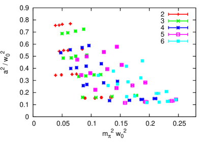
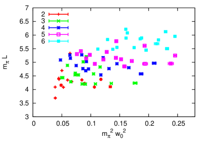
Figure 1: The landscape of simulation points for the various flavor numbers $N_{f}$. Left: cut-off and Goldstone mass. Right: volume and Goldstone mass.

The observables we measure are $m_{\pi},f_{\pi},m_{\varrho},w_{0}$ and the topological susceptibility $Q^{2}/V$. The scale $w_{0}$ Borsanyi:2012zs is measured using the SSC discretization according to the terminology in Fodor:2014cpa . For each $N_{f}$ simulations were carried out at four lattice spacings and four fermion masses at each lattice spacing giving a total of 16 points; these are tabulated in tables 3 and 4. The total number of thermalized trajectories is $1000-2500$ and every $10^{th}$ is used for measurements.

The landscape of simulation points in terms of cut-off, Goldstone mass and volume is shown in figure 1.

3 Finite volume effects

The simulations are performed in finite volume and the associated systematic errors ought to be controlled. In order to have fully controlled finite volume effects two issues need to be addressed. One, it is important to be in the kinematical regime where the $\varrho$-meson can not decay into pions. Hence all simulations were performed in the regime such that $m_{\varrho}/(2m_{\pi})<\sqrt{1+\left(\frac{2\pi}{m_{\pi}L}\right)^{2}}$. This constraint mainly prevents us from reaching too light fermion masses at rough lattice spacings. Two, the topological charge should fluctuate enough and should not be frozen so as not to have approximately fixed topology simulations. This constraint is most relevant at small lattice spacings and we made sure that topology does change frequently enough even at the finest lattice spacings we use. The topology change is frequent enough such that we are able to measure the topological susceptibility for all runs and the expectations from tree level chiral perturbation theory are confirmed (see next section).

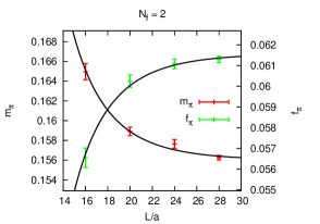
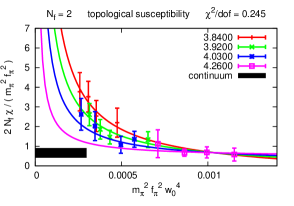
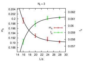
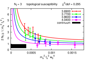
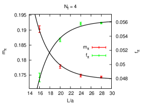
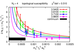
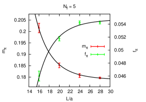
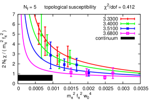
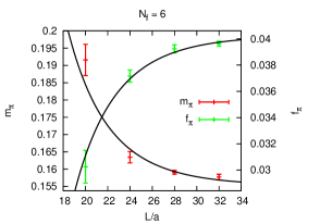
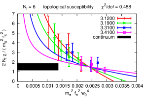
Figure 2: Left: infinite volume extrapolations of $m_{\pi}$ and $f_{\pi}$, based on table 2. Right: chiral-continuum extrapolation of the topological susceptibility. The ratio $2N_{f}\chi/(m_{\pi}^{2}f_{\pi}^{2})$ is shown which is expected to be constant $1$ at leading order of chiral perturbation theory; see text for more details.

Once these two issues are handled properly the finite volume effects in $m_{\pi}$ and $f_{\pi}$ are purely exponential in $m_{\pi}L$. The residual finite volume effect in $m_{\varrho}$ can be estimated based on the relationship between finite volume energy levels and scattering states Luscher:1990ux ; Luscher:1991cf .

How large $m_{\pi}L$ needs to be in order to have a fixed small finite volume effect in $m_{\pi}$ and $f_{\pi}$, e.g. less than $1\%$, depends on $N_{f}$. For each flavor number we have performed dedicated finite volume runs at fixed lattice spacing and fermion mass. The infinite volume extrapolation is through the non-linear fit

$$m_{\pi}(L) = m_{\pi\infty}+C_{m}\;g(m_{\pi\infty}L)$$ (1)

where the fit parameters are $m_{\pi\infty}$ and $C_{m}$. The form of the finite volume correction Gasser:1986vb is given by

$$g(x) = \frac{4}{x}\sum_{n\neq 0}\frac{K_{1}(nx)}{n}$$ (2)

with the modified Bessel function of the second kind $K_{1}$ and the sum is over integers $(n_{1},n_{2},n_{3},n_{4})$ such that $n^{2}=n_{1}^{2}+n_{2}^{2}+n_{3}^{2}+4n_{4}^{2}\neq 0$; see also Colangelo:2005gd . The sum may be replaced by the first exponential and all infinite volume extrapolations were repeated as a cross-check with a single exponential and give identical results, within errors, to the one obtained using the full $g(x)$ function.

Using the $m_{\pi}(L)$ data the infinite volume extrapolated $m_{\pi\infty}$ and its error may be obtained. Once this is done the decay constant $f_{\pi}(L)$ needs to be extrapolated as well, using a similar expression Gasser:1986vb ,

$$f_{\pi}(L) = f_{\pi\infty}-C_{f}\;g(m_{\pi\infty}L)$$ (3)

where now the fit is linear in the fit parameters $f_{\pi\infty}$ and $C_{f}$. The statistical error on $m_{\pi\infty}$ does need to be propagated carefully into the above fit of course. Note that $C_{f}>0$ and $C_{m}>0$, i.e. masses decrease towards larger volumes while the decay constant increases. The net effect on the ratio $m_{\varrho}/f_{\pi}$ is an enhancement of finite volume effects.

Our results for all flavor numbers are shown in figure 2 (left) based on the data in table 2. The main conclusion is that in order to have a fixed small finite volume effect, $m_{\pi}L$ needs to grow linearly with $N_{f}$. For instance in order to have less than $1\%$ finite volume effects in $m_{\pi}$ and $f_{\pi}$ the following needs to hold for the spatial volume,

$$m_{\pi}L>3.10+0.35N_{f}\;.$$ (4)

Clearly, as $N_{f}$ is increasing finite volume effects get larger. The conventional rule of thumb $m_{\pi}L>4$ from QCD is satisfactory for sub-percent finite volume effects at $N_{f}=2,3$ but for $N_{f}=4,5,6$ it is not. For instance at $N_{f}=6$ one needs $m_{\pi}L>5.2$. As the fermion content gets larger and the model moves closer to the conformal window finite volume effects grow, in line with general expectations. Here we have quantified this phenomenon for $SU(3)$ and fundamental fermions.

In our runs condition (4) is satisfied which means that our chiral extrapolations are essentially in infinite volume. The chiral expansion in infinite volume Gasser:1984gg is indeed applicable to the simulations once $f_{\pi}L$ is large enough. For all our simulations we have $0.95\leq f_{\pi}L\leq 1.92$. Note that our $f_{\pi}$ is in the “lower” convention, i.e. the one which gives $f_{\pi}\approx 92\;MeV$ and not $130\;MeV$, in QCD.

Finite volume effects in $m_{\varrho}$ can be estimated a posteriori as follows. Using the KSRF-relation (9) we determine $g_{\varrho\pi\pi}$ for each $N_{f}$. Once $g_{\varrho\pi\pi}$ is fixed the finite volume effects are given by the relationship between finite volume energy levels and scattering states Luscher:1990ux ; Luscher:1991cf and $m_{\varrho}$ in infinite volume can be obtained from a single volume as is the case for us. The result here is that finite volume effects are at most 2% at 12 out of the 16 simulation points at $N_{f}=2$, are at most 2% at all 16 simulation points at $N_{f}=3$, are at most 1% at 15 out of the 16 simulation points at $N_{f}=4$ and at most 1% for all points at $N_{f}=5$ and $N_{f}=6$. Our final statistical uncertainties for $w_{0}m_{\varrho}$ are between 3% and 5% hence we conclude a posteriori that finite volume effects for all of our observables are under control.

4 Chiral-continuum extrapolation

Before discussing the chiral-continuum extrapolations it is worth remembering that staggered fermions, as is well-known, suffer from taste breaking. This means that the measured pseudo-scalar meson is the lightest of the full taste broken multiplet and the higher ones ($N_{f}^{2}-2$ of them) do not chirally extrapolate to zero at fixed non-zero lattice spacing. In other words the chiral $SU(N_{f})\times SU(N_{f})$ group is broken at finite lattice spacing and the $N_{f}$-dependence of low energy observables on the lattice is not necessarily the same as in the continuum, only if the lattice spacing is small enough and all Goldstone bosons are light enough. Hence before attempting to extrapolate both chirally and to the continuum our main observable, the $m_{\varrho}/f_{\pi}$ ratio, we sought a quantity which is as sensitive to $N_{f}$ as possible in order to test whether our simulations are close enough to the continuum and zero fermion mass limit.

4.1 Topological susceptibility

A powerful test of whether at finite lattice spacing the effective number of light degrees of freedom is the same as in the continuum is given by the topological susceptibility. The topological susceptibility is very sensitive to the light degrees of freedom since these are the ones at small fermion mass which suppress non-zero topology. As a result $N_{f}$-dependence shows up already at the leading order of chiral perturbation theory Leutwyler:1992yt ,

$$\frac{\langle Q^{2}\rangle}{V}=\chi=\frac{1}{2N_{f}}f_{\pi}^{2}m_{\pi}^{2}$$ (5)

i.e. the $N_{f}$-dependence is fixed once $m_{\pi}$ and $f_{\pi}$ are measured. We have performed a combined chiral-continuum extrapolation of the topological susceptibility for each $N_{f}$ and have confirmed the above expectation, indicating that the light degrees of freedom are correctly captured, i.e. any deviation from the continuum due to taste broken Goldstone bosons is correctly extrapolated to zero as $O(a^{2})$. This is a highly non-trivial test for each $N_{f}$ and we take it to indicate that the lattice spacings and bare fermion masses were indeed chosen such that a combined chiral-continuum extrapolation is meaningful.

More precisely, we use the gradient flow based Luscher:2010iy discretization of the topological charge, measuring it at $t=w_{0}^{2}$. Note that the chiral extrapolation of $\chi$ at finite lattice spacing does not need to vanish, precisely because of the fact that the taste broken Goldstone bosons do not extrapolate to zero Billeter:2004wx . Hence we adopt the following combined chiral-continuum extrapolation at each $N_{f}$,

$$\chi w_{0}^{4}=C_{0}m_{\pi}^{2}f_{\pi}^{2}w_{0}^{4}+C_{1}\frac{a^{2}}{w_{0}^{2}}+C_{2}\frac{a^{2}}{w_{0}^{2}}(m_{\pi}^{2}f_{\pi}^{2}w_{0}^{4})\;,$$ (6)

where the fit parameters are $C_{0},C_{1}$ and $C_{2}$. The continuum expectation (5) is then $C_{0}=1/(2N_{f})$. In figure 2 (right) we plot the ratio $2N_{f}\chi/(m_{\pi}^{2}f_{\pi}^{2})$ for each $N_{f}$ which ought to be consistent with the constant $1$ in the chiral continuum limit. At each $\beta$ we also fit $a^{2}/w_{0}^{2}$ as a linear function of $m_{\pi}^{2}f_{\pi}^{2}w_{0}^{4}$ and then using the fitted $C_{0,1,2}$ coefficients together with (6) we also show the resulting mass dependence at each $\beta$ by the solid lines in order to get a sense of the size of cut-off effects. The extrapolated $2N_{f}C_{0}$ coefficient is shown by the black bands, these are $0.67(24)$, $0.65(33)$, $0.59(28)$, $0.60(29)$ and $1.51(36)$ for $N_{f}=2,3,4,5,6$, respectively. We find that for all $N_{f}$ there is agreement with $1$ within at most $1.5\,\sigma$, which is even though not perfect, certainly better than expected since we only fit the leading order expression. All $\chi^{2}/dof$ (with $dof=13$) of the extrapolations are below unity.

4.2 The $m_{\varrho}/f_{\pi}$ ratio

Having quantitative confirmation that taste breaking effects scale to zero as $O(a^{2})$ as expected we turn to the main object of our study, the $m_{\varrho}/f_{\pi}$ ratio. In order to estimate the systematic error coming from the chiral-continuum extrapolation we have performed two types of fits.

In the first one, at each $N_{f}$ the decay constant and the $\varrho$ mass are extrapolated separately to the chiral-continuum limit in $w_{0}$ units. Concretely, the extrapolation is via

$$Xw_{0}=C_{0}+C_{1}m_{\pi}^{2}w_{0}^{2}+C_{2}\frac{a^{2}}{w_{0}^{2}}+C_{3}\frac{a^{2}}{w_{0}^{2}}m_{\pi}^{2}w_{0}^{2}$$ (7)

where $X$ is either $m_{\varrho}$ or $f_{\pi}$ and there are four fit parameters $C_{0,1,2,3}$ hence $dof=12$ for each $N_{f}$. In this procedure we obtain $f_{\pi}w_{0}$ and $m_{\varrho}w_{0}$ in the chiral-continuum limit at each $N_{f}$ and the results are given in table 1 together with the $\chi^{2}/dof$ values. The extrapolations are shown in figure 3 where the chiral-continuum final results are shown in black together with the measured data. The solid lines corresponding to each bare $\beta$ were obtained by fitting the scale $a^{2}/w_{0}^{2}$ as a linear function of $m_{\pi}^{2}w_{0}^{2}$ together with equation (7). Clearly cut-off effects are small which is due to our choice of discretization and the choice of $w_{0}$ to set the scale.

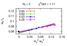
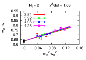
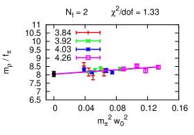
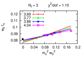
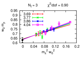
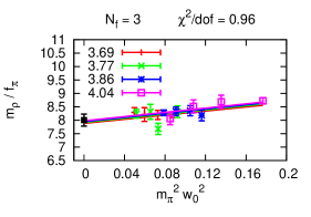
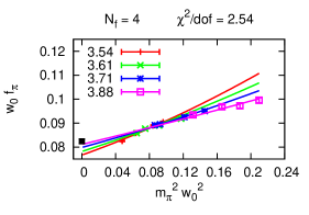
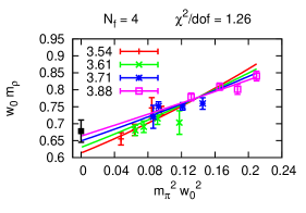
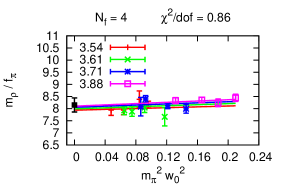
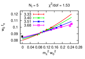
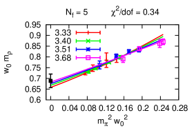
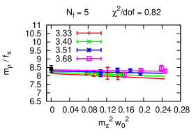
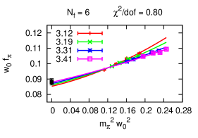
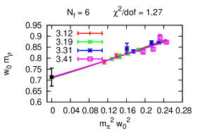
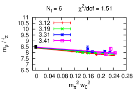
Figure 3: Chiral-continuum extrapolation of $f_{\pi}w_{0}$, $m_{\varrho}w_{0}$ (left two columns) and directly the ratio $m_{\varrho}/f_{\pi}$ (right most column) for $N_{f}=2,3,4,5$ and $6$, from top to bottom, respectively. Equations (7) and (8) are used and the resulting $\chi^{2}/dof$ is shown at the top of each plot. The various colors correspond to different lattice spacings (i.e. different bare $\beta$) and were obtained by interpolations of $a^{2}/w_{0}^{2}$ as a linear function of $m_{\pi}^{2}w_{0}^{2}$ together with equations (7) and (8); see text for more details.

In the second procedure the ratio is fitted directly via

$$\frac{m_{\varrho}}{f_{\pi}}=C_{0}+C_{1}m_{\pi}^{2}w_{0}^{2}+C_{2}\frac{a^{2}}{w_{0}^{2}}$$ (8)

where now we have three fit parameters $C_{0,1,2}$ hence $dof=13$ for all $N_{f}$. The results are shown again in figure 3. Clearly, both cut-off and mass effects are remarkably small for the ratio although the mass-dependence of both $m_{\varrho}w_{0}$ and $f_{\pi}w_{0}$ are much larger in comparison.

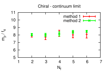
Figure 4: Our final results for the ratio $m_{\varrho}/f_{\pi}$ in the chiral-continuum limit for each $N_{f}$. Two procedures are used for the chiral-continuum extrapolation in order to assess systematic errors; the two agrees within errors. Method one is our final result and method two serves as a cross-check or confirmation.

$N_{f}$	$f_{\pi}w_{0}$	$m_{\varrho}w_{0}$	$m_{\varrho}/f_{\pi}$
2	0.0801(5)	0.64(2)	7.9(2)
3	0.082(1)	0.63(3)	7.7(3)
4	0.0824(9)	0.68(3)	8.2(4)
5	0.086(1)	0.69(3)	8.0(4)
6	0.088(2)	0.71(4)	8.1(5)

Table 1: Continuum results for each $N_{f}$ in the chiral limit.

The above two procedures give compatible results for $m_{\varrho}/f_{\pi}$ within errors, the final results are shown in figure 4. The final errors are dominated by the errors on $m_{\varrho}$, the errors on $f_{\pi}$ are negligible in comparison. We take the results from the first procedure as our final continuum results and use the second procedure, with its much smaller error, as confirmation or cross-check.

Our main conclusion can be drawn from figure 4; the $N_{f}$-dependence of the ratio $m_{\varrho}/f_{\pi}$ is remarkably small. We may even fit the results to a constant and obtain acceptable statistical fits. Using the first procedure one obtains $m_{\varrho}/f_{\pi}=7.95(15)$ whereas the second procedure leads to $m_{\varrho}/f_{\pi}=8.28(8)$, with $\chi^{2}/dof=0.26$ and $1.69$, respectively. The agreement is within $2\,\sigma$.

This largely $N_{f}$-independent behavior is consistent with the observation that at each $N_{f}$ the mass-dependence of the ratio is also very small. In addition note that free fermions have $m_{\varrho}=2m$ as is the case for any meson and also $f_{\pi}=\sqrt{12}m$ Cichy:2008gk , leading to a very small ratio $m_{\varrho}/f_{\pi}=1/\sqrt{3}$. This result in the free theory can be thought of as the relevant ratio at $N_{f}=33/2$ at the upper end of the conformal window. Hence we conclude that well below the conformal window, $2\leq N_{f}\leq 6$ the ratio is relatively stable at around $\sim 8.0$ and somewhere in the range $7\leq N_{f}\leq 16.5$ it drops an order of magnitude to $\sim 0.6$. The extension of our work to this remaining range $7\leq N_{f}\leq 16.5$ is left for future work and we believe that once it is completed it may serve as valuable insight into the appearance of the conformal window, presumably at around $N_{f}\sim 13$. Note that inside the conformal window the chiral limit of the ratio $m_{\varrho}/f_{\pi}$ is understood similarly to the free theory; both the numerator and the denominator is finite at finite fermion mass with a well-defined ratio in the chiral limit.

5 Conclusion and outlook

In this work we have determined the $m_{\varrho}/f_{\pi}$ ratio in the chiral-continuum limit of $SU(3)$ gauge theory coupled to $N_{f}=2,3,4,5,6$ fermions in the fundamental representation in such a way that all systematic errors are fully controlled. A remarkable $N_{f}$-independence is observed with $m_{\varrho}/f_{\pi}=7.95(15)$ while several quantities do show non-trivial $N_{f}$-dependence. The motivation for our study was that in a large class of strongly interacting extensions of the Standard Model the experimentally most easily accessible new composite particle is the vector resonance. The scale in these models is set by $f_{\pi}=246\;GeV$ hence we are led to conclude that as long as the gauge group is chosen to be $SU(3)$ the first resonance ought to be at around $\sim 2\;TeV$ independent of the specific fermion content of the theory.

Our result is not only a robust prediction for the mass of the vector resonance but also a host of other related quantities. The KSRF-relations Kawarabayashi:1966kd ; Riazuddin:1966sw establish relationships among the vector mass, its width $\Gamma_{\varrho}$ and decay constant $f_{\varrho}$ and the $\varrho\pi\pi$ coupling $g_{\rho\pi\pi}$. Specifically,

$$g_{\varrho\pi\pi} = \frac{m_{\varrho}}{f_{\varrho}}=\sqrt{48\pi\frac{\Gamma_{\varrho}}{m_{\varrho}}}=\frac{1}{\sqrt{2}}\frac{m_{\varrho}}{f_{\pi}}\;.$$ (9)

The assumptions underlying the KSRF-relations are the applicability of leading order chiral perturbation theory, vector meson dominance and vector meson universality. The last two conditions completely determine the way the vector resonance ought to appear in the chiral Lagrangian and simple leading order calculations lead to the above relations; see Bando:1987br for a review. These relations are surprisingly accurate in QCD and it is expected that they become even more accurate closer to the chiral limit. Hence our result for an approximately $N_{f}$-independent ratio $m_{\varrho}/f_{\pi}$ leads to similar results for the coupling $g_{\varrho\pi\pi}$ and the $\varrho$ width and decay constant in $m_{\varrho}$ units. In a strong dynamics inspired composite Higgs scenario this means $\Gamma_{\varrho}\sim 410\;GeV$, $f_{\varrho}\sim 348\;GeV$ and $g_{\varrho\pi\pi}\sim 5.62$, independently of the details of the fermion content as long as $SU(3)$ is the gauge group. These additional results are especially useful because a direct lattice calculation of $g_{\varrho\pi\pi}$ or $\Gamma_{\varrho}$ is very challenging.

Note that the KSRF-relations merely relate $m_{\varrho}/f_{\pi}$ to other quantities in the given theory at fixed $N_{f}$. Hence even if the validity of the KSRF-relations is accepted it is not at all clear why this particular ratio is insensitive to $N_{f}$ and it would be welcome to derive it at least approximately from first principles.

The above is especially true since the change in the detailed dynamics of gauge theory as $N_{f}$ is varied is highly non-trivial. As $N_{f}$ grows, the number of massless particles increases, the running of the renormalized coupling slows down, the $S$-parameter increases but $S/N_{f}$ decreases Appelquist:2010xv ; Appelquist:2014zsa , the topological susceptibility decreases in $m_{\pi}^{2}f_{\pi}^{2}$ units, the mass of the $O^{++}$ scalar in $f_{\pi}$ units decreases Aoki:2013zsa ; Aoki:2014oha ; Rinaldi:2015axa ; Fodor:2016pls ; Aoki:2016wnc ; Appelquist:2016viq , yet the vector meson related quantities stay roughly constant. It would be interesting to see how $m_{\varrho}/f_{\pi}$ changes across the lower end of the conformal window, presumably close to $N_{f}\sim 13$ and how the free value $1/\sqrt{3}$ is reached at $N_{f}=33/2$ at the upper end of the conformal window. For this investigation the starting point must be the extension of the result (4) to $N_{f}\geq 7$ because it is not at all guaranteed that (4) holds for flavor numbers beyond the range considered in this work.

It should be noted that lattice results indicate that $m_{\varrho}/f_{\pi}$ is not completely universal, it does depend on the gauge group. Evidence comes from $SU(2)$ simulations with $N_{f}=2,4$ fundamental fermions. With $N_{f}=2$ continuum results Lewis:2011zb ; Arthur:2016dir ; Drach:2017btk are available in the chiral limit, $m_{\varrho}/f_{\pi}\sim 15$ while with $N_{f}=4$ results at finite lattice spacing Amato:2018nvj indicate $m_{\varrho}/f_{\pi}>10$. It would be worthwhile to obtain fully controlled continuum results with $SU(2)$ at $N_{f}=2,3,4$ and perhaps $N_{f}=5$ in order to see whether the $N_{f}$-independence below the conformal window we have seen for $SU(3)$ is also present with $SU(2)$ or not. In any case a larger $m_{\varrho}/f_{\pi}$ ratio for $SU(2)$ relative to $SU(3)$ is in line with large-$N$ scaling arguments since $m_{\varrho}\sim O(1)$ while $f_{\pi}\sim O(\sqrt{N})$; see Bali:2013kia ; DeGrand:2016pur and references therein.

6 Data tables

$N_{f}$	$\beta$	$m$	$L/a$	$am_{\pi}$	$af_{\pi}$
2	3.92	0.0075	16	0.1650(8)	0.0565(5)
			20	0.1589(4)	0.0602(3)
			24	0.1577(4)	0.0611(2)
			28	0.1563(2)	0.0613(2)
			$\infty$	0.1560(3)    1.11	0.0616(2)    0.48
3	3.77	0.0110	16	0.199(1)	0.0577(4)
			20	0.1929(7)	0.0603(4)
			24	0.1916(8)	0.0612(2)
			28	0.1904(4)	0.0612(2)
			$\infty$	0.1902(4)    0.28	0.0613(2)    0.24
4	3.61	0.0088	16	0.190(1)	0.0482(6)
			20	0.1779(6)	0.0535(2)
			24	0.1748(5)	0.0558(2)
			28	0.1743(3)	0.0559(1)
			$\infty$	0.1734(3)    0.97	0.0563(2)    2.62
5	3.40	0.0085	16	0.202(2)	0.0460(8)
			20	0.185(1)	0.0518(3)
			24	0.1807(9)	0.0543(3)
			28	0.1797(3)	0.0543(2)
			$\infty$	0.1788(6)    0.15	0.0548(2)    2.04
6	3.31	0.0080	20	0.192(5)	0.030(1)
			24	0.163(2)	0.0372(5)
			28	0.1591(5)	0.0392(3)
			32	0.1577(8)	0.0396(2)
			$\infty$	0.155(1)    2.87	0.0403(3)    0.87

Table 2: Volume dependence of $m_{\pi}$ and $f_{\pi}$. The infinite volume extrapolated result is also shown together with the $\chi^{2}/dof$ of the extrapolations; $dof=2$.

$N_{f}$	$\beta$	$m$	$L/a$	$am_{\pi}$	$af_{\pi}$	$am_{\varrho}$	$w_{0}/a$	$10^{4}a^{4}\chi$
2	3.84	0.0130	24	0.2221(1)	0.1066(3)	0.61(2)	1.140(1)	1.5(3)
		0.0100	24	0.1957(2)	0.1037(2)	0.58(2)	1.144(1)	1.3(2)
		0.0088	24	0.1839(2)	0.1020(2)	0.59(2)	1.1493(6)	1.5(2)
		0.0075	24	0.1704(2)	0.1006(2)	0.61(1)	1.151(1)	1.4(2)
	3.92	0.0147	20	0.2177(6)	0.0929(3)	0.548(6)	1.337(3)	0.7(1)
		0.0100	24	0.1812(3)	0.0889(2)	0.524(8)	1.351(2)	0.47(6)
		0.0088	24	0.1701(2)	0.0885(2)	0.517(6)	1.350(2)	0.53(7)
		0.0075	28	0.1563(2)	0.0867(2)	0.501(4)	1.360(1)	0.60(6)
	4.03	0.0100	28	0.1624(4)	0.0737(3)	0.424(4)	1.683(2)	0.24(4)
		0.0088	28	0.1533(4)	0.0720(4)	0.420(6)	1.689(3)	0.16(3)
		0.0062	32	0.1300(9)	0.0700(1)	0.403(3)	1.700(2)	0.21(4)
		0.0050	32	0.1153(3)	0.0686(2)	0.402(6)	1.708(2)	0.21(3)
	4.26	0.0115	28	0.1465(8)	0.0526(3)	0.314(3)	2.50(1)	0.04(1)
		0.0100	32	0.1367(5)	0.0519(4)	0.302(4)	2.508(7)	0.043(9)
		0.0088	32	0.1279(4)	0.0500(2)	0.302(2)	2.550(7)	0.034(5)
		0.0075	36	0.1173(4)	0.0494(4)	0.292(2)	2.55(1)	0.05(1)
3	3.69	0.0158	20	0.2509(5)	0.1061(3)	0.614(6)	1.175(2)	1.2(2)
		0.0130	20	0.2271(4)	0.1032(2)	0.60(1)	1.189(2)	1.4(2)
		0.0105	24	0.2036(3)	0.1002(3)	0.58(2)	1.200(1)	1.1(1)
		0.0085	24	0.1849(4)	0.0974(2)	0.57(1)	1.206(1)	1.0(1)
	3.77	0.0140	24	0.2168(3)	0.0898(2)	0.53(1)	1.402(2)	0.65(6)
		0.0110	24	0.1916(8)	0.0865(3)	0.47(1)	1.413(2)	0.54(8)
		0.0095	24	0.1786(5)	0.0840(3)	0.49(2)	1.434(2)	0.55(7)
		0.0075	28	0.1584(2)	0.0828(2)	0.48(1)	1.436(2)	0.35(6)
	3.86	0.0145	24	0.2012(6)	0.0762(4)	0.44(1)	1.694(5)	0.22(4)
		0.0130	24	0.1906(4)	0.0747(3)	0.44(1)	1.698(6)	0.23(3)
		0.0110	24	0.1750(7)	0.0723(4)	0.426(8)	1.722(5)	0.18(3)
		0.0095	28	0.1620(2)	0.0715(2)	0.418(5)	1.732(4)	0.22(5)
	4.04	0.0150	24	0.177(1)	0.0562(6)	0.347(3)	2.38(2)	0.07(2)
		0.0111	28	0.1509(6)	0.0537(4)	0.330(9)	2.44(1)	0.07(1)
		0.0085	32	0.1314(7)	0.0505(3)	0.304(8)	2.50(1)	0.05(1)
		0.0067	36	0.1168(5)	0.0497(3)	0.283(8)	2.498(8)	0.022(5)
4	3.54	0.0140	20	0.2378(5)	0.0981(3)	0.566(9)	1.304(3)	0.8(1)
		0.0120	24	0.2198(4)	0.0952(2)	0.56(2)	1.323(2)	0.8(1)
		0.0088	28	0.1882(3)	0.0903(2)	0.51(1)	1.344(2)	0.8(1)
		0.0062	32	0.1589(2)	0.0849(2)	0.48(1)	1.375(2)	0.6(1)
	3.61	0.0146	20	0.2269(7)	0.0860(3)	0.47(2)	1.511(5)	0.51(7)
		0.0110	24	0.1955(5)	0.0814(3)	0.46(1)	1.546(5)	0.28(5)
		0.0088	28	0.1743(3)	0.0790(2)	0.44(1)	1.570(2)	0.41(3)
		0.0075	32	0.1609(1)	0.0767(1)	0.43(1)	1.583(2)	0.34(4)
	3.71	0.0151	24	0.2062(7)	0.0727(4)	0.411(9)	1.849(9)	0.22(3)
		0.0121	28	0.1846(4)	0.0693(3)	0.398(6)	1.888(7)	0.16(4)
		0.0088	32	0.1572(3)	0.0654(2)	0.388(7)	1.936(5)	0.13(2)
		0.0080	32	0.1490(3)	0.0639(2)	0.37(2)	1.972(6)	0.12(2)
	3.88	0.0150	28	0.1774(7)	0.0546(5)	0.326(5)	2.58(2)	0.06(1)
		0.0130	28	0.163(1)	0.0520(5)	0.303(5)	2.65(2)	0.032(6)
		0.0110	32	0.1501(6)	0.0505(3)	0.298(4)	2.71(1)	0.022(3)
		0.0088	36	0.1324(8)	0.0483(2)	0.284(4)	2.74(1)	0.030(4)

Table 3: Data for $N_{f}=2,3,4$.

$N_{f}$	$\beta$	$m$	$L/a$	$am_{\pi}$	$af_{\pi}$	$am_{\varrho}$	$w_{0}/a$	$10^{4}a^{4}\chi$
5	3.33	0.0190	20	0.2888(4)	0.1070(4)	0.60(1)	1.314(3)	1.3(3)
		0.0148	20	0.2553(4)	0.0995(4)	0.57(2)	1.367(5)	0.9(1)
		0.0105	24	0.2144(3)	0.0917(2)	0.53(1)	1.416(3)	0.8(1)
		0.0081	28	0.1894(2)	0.0861(2)	0.498(6)	1.456(2)	0.67(7)
	3.40	0.0168	20	0.2555(5)	0.0915(4)	0.522(5)	1.527(4)	0.7(1)
		0.0131	24	0.2242(5)	0.0855(2)	0.486(2)	1.594(4)	0.42(7)
		0.0093	28	0.1884(5)	0.0783(4)	0.449(4)	1.665(4)	0.43(6)
		0.0075	32	0.1690(3)	0.0746(2)	0.430(5)	1.704(3)	0.39(9)
	3.51	0.0174	24	0.2337(8)	0.0771(5)	0.443(4)	1.88(1)	0.18(2)
		0.0142	24	0.2104(7)	0.0713(3)	0.419(5)	1.966(9)	0.21(4)
		0.0110	28	0.1845(4)	0.0662(4)	0.391(5)	2.053(7)	0.14(2)
		0.0079	32	0.1545(3)	0.0624(2)	0.360(9)	2.117(7)	0.13(3)
	3.68	0.0153	28	0.1874(6)	0.0562(3)	0.329(5)	2.65(1)	0.06(2)
		0.0135	28	0.1770(9)	0.0523(4)	0.313(6)	2.76(2)	0.028(4)
		0.0104	32	0.155(1)	0.0500(3)	0.294(3)	2.85(2)	0.034(6)
		0.0082	36	0.1347(8)	0.0469(3)	0.268(5)	2.95(2)	0.023(4)
6	3.12	0.0192	20	0.2947(5)	0.1025(3)	0.569(3)	1.471(5)	0.6(1)
		0.0150	24	0.2590(3)	0.0945(2)	0.534(5)	1.547(4)	0.9(1)
		0.0117	24	0.2283(4)	0.0866(4)	0.497(6)	1.628(6)	0.6(1)
		0.0086	28	0.1960(3)	0.07939(7)	0.458(5)	1.710(5)	0.51(8)
	3.19	0.0150	24	0.2442(6)	0.0842(3)	0.476(3)	1.763(6)	0.42(5)
		0.0120	28	0.2171(3)	0.0783(3)	0.441(4)	1.861(7)	0.30(6)
		0.0100	28	0.1981(4)	0.0739(3)	0.420(5)	1.924(6)	0.29(4)
		0.0085	32	0.1824(3)	0.0706(1)	0.405(3)	1.969(5)	0.31(5)
	3.31	0.0150	28	0.2187(8)	0.0701(2)	0.398(2)	2.190(8)	0.19(3)
		0.0125	28	0.203(1)	0.0667(5)	0.382(3)	2.28(1)	0.12(2)
		0.0095	32	0.1731(2)	0.0602(2)	0.344(3)	2.42(1)	0.14(2)
		0.0085	36	0.1636(3)	0.0584(1)	0.34(1)	2.452(7)	0.11(2)
	3.41	0.0130	32	0.1860(5)	0.0581(2)	0.328(2)	2.663(9)	0.056(7)
		0.0112	32	0.1719(6)	0.0542(3)	0.319(5)	2.80(1)	0.042(5)
		0.0100	36	0.1618(3)	0.0525(2)	0.292(3)	2.880(9)	0.05(1)
		0.0089	36	0.1513(5)	0.0507(3)	0.284(3)	2.92(1)	0.045(9)

Table 4: Data for $N_{f}=5,6$.

References

- (1)
- (2) Z. Fodor, K. Holland, J. Kuti, D. Nogradi and C. Schroeder, Phys. Lett. B 681, 353 (2009) [arXiv:0907.4562 [hep-lat]].
- (3) X. Y. Jin and R. D. Mawhinney, PoS LAT 2009, 049 (2009) [arXiv:0910.3216 [hep-lat]].
- (4) Y. Aoki et al. [LatKMI Collaboration], Phys. Rev. D 87, no. 9, 094511 (2013) [arXiv:1302.6859 [hep-lat]].
- (5) X. Y. Jin and R. D. Mawhinney, arXiv:1304.0312 [hep-lat].
- (6) G. T. Fleming et al. [LSD Collaboration], arXiv:1312.5298 [hep-lat].
- (7) T. Appelquist et al., Phys. Rev. D 93, no. 11, 114514 (2016) [arXiv:1601.04027 [hep-lat]].
- (8) T. Appelquist et al. [Lattice Strong Dynamics Collaboration], Phys. Rev. D 99, no. 1, 014509 (2019) [arXiv:1807.08411 [hep-lat]].
- (9) Z. Fodor, K. Holland, J. Kuti, D. Nogradi, C. Schroeder and C. H. Wong, Phys. Lett. B 718, 657 (2012) [arXiv:1209.0391 [hep-lat]].
- (10) Z. Fodor, K. Holland, J. Kuti, S. Mondal, D. Nogradi and C. H. Wong, PoS LATTICE 2015, 219 (2016) [arXiv:1605.08750 [hep-lat]].
- (11) Z. Fodor, K. Holland, J. Kuti, S. Mondal, D. Nogradi and C. H. Wong, Phys. Rev. D 94, no. 1, 014503 (2016) [arXiv:1601.03302 [hep-lat]].
- (12) K. Kawarabayashi and M. Suzuki, Phys. Rev. Lett. 16, 255 (1966).
- (13) Riazuddin and Fayyazuddin, Phys. Rev. 147, 1071 (1966).
- (14) K. Cichy, J. Gonzalez Lopez, K. Jansen, A. Kujawa and A. Shindler, Nucl. Phys. B 800, 94 (2008) [arXiv:0802.3637 [hep-lat]].
- (15) C. Morningstar and M. J. Peardon, Phys. Rev. D 69, 054501 (2004) [hep-lat/0311018].
- (16) S. Durr et al., JHEP 1108, 148 (2011) [arXiv:1011.2711 [hep-lat]].
- (17) Z. Fodor, K. Holland, J. Kuti, D. Nogradi and C. H. Wong, JHEP 1211, 007 (2012) [arXiv:1208.1051 [hep-lat]].
- (18) Z. Fodor, K. Holland, J. Kuti, S. Mondal, D. Nogradi and C. H. Wong, JHEP 1506, 019 (2015) [arXiv:1503.01132 [hep-lat]].
- (19) Z. Fodor, K. Holland, J. Kuti, S. Mondal, D. Nogradi and C. H. Wong, JHEP 1509, 039 (2015) [arXiv:1506.06599 [hep-lat]].
- (20) Z. Fodor, K. Holland, J. Kuti, D. Nogradi and C. H. Wong, EPJ Web Conf. 175, 08027 (2018) [arXiv:1711.04833 [hep-lat]].
- (21) S. Duane, A. D. Kennedy, B. J. Pendleton and D. Roweth, Phys. Lett. B 195, 216 (1987).
- (22) M. A. Clark and A. D. Kennedy, Phys. Rev. Lett. 98, 051601 (2007) [hep-lat/0608015].
- (23) J. C. Sexton and D. H. Weingarten, Nucl. Phys. B 380, 665 (1992).
- (24) T. Takaishi and P. de Forcrand, Phys. Rev. E 73, 036706 (2006) [hep-lat/0505020].
- (25) S. Borsanyi et al., JHEP 1209, 010 (2012) [arXiv:1203.4469 [hep-lat]].
- (26) Z. Fodor, K. Holland, J. Kuti, S. Mondal, D. Nogradi and C. H. Wong, JHEP 1409, 018 (2014) [arXiv:1406.0827 [hep-lat]].
- (27) M. Luscher, Nucl. Phys. B 354, 531 (1991).
- (28) M. Luscher, Nucl. Phys. B 364, 237 (1991).
- (29) J. Gasser and H. Leutwyler, Phys. Lett. B 184, 83 (1987).
- (30) G. Colangelo, S. Durr and C. Haefeli, Nucl. Phys. B 721, 136 (2005) [hep-lat/0503014].
- (31) J. Gasser and H. Leutwyler, Nucl. Phys. B 250, 465 (1985).
- (32) H. Leutwyler and A. V. Smilga, Phys. Rev. D 46, 5607 (1992).
- (33) M. Lüscher, JHEP 1008, 071 (2010) Erratum: [JHEP 1403, 092 (2014)] [arXiv:1006.4518 [hep-lat]].
- (34) B. Billeter, C. E. Detar and J. Osborn, Phys. Rev. D 70, 077502 (2004) [hep-lat/0406032].
- (35) M. Bando, T. Kugo and K. Yamawaki, Phys. Rept. 164, 217 (1988).
- (36) Z. Komargodski, JHEP 1102, 019 (2011) [arXiv:1010.4105 [hep-th]].
- (37) T. Appelquist et al. [LSD Collaboration], Phys. Rev. Lett. 106, 231601 (2011) [arXiv:1009.5967 [hep-ph]].
- (38) T. Appelquist et al. [LSD Collaboration], Phys. Rev. D 90, no. 11, 114502 (2014) [arXiv:1405.4752 [hep-lat]].
- (39) Y. Aoki et al. [LatKMI Collaboration], Phys. Rev. Lett. 111, no. 16, 162001 (2013) [arXiv:1305.6006 [hep-lat]].
- (40) Y. Aoki et al. [LatKMI Collaboration], Phys. Rev. D 89, 111502 (2014) [arXiv:1403.5000 [hep-lat]].
- (41) E. Rinaldi [LSD Collaboration], Int. J. Mod. Phys. A 32, no. 35, 1747002 (2017) [arXiv:1510.06771 [hep-lat]].
- (42) Y. Aoki et al. [LatKMI Collaboration], Phys. Rev. D 96, no. 1, 014508 (2017) [arXiv:1610.07011 [hep-lat]].
- (43) R. Lewis, C. Pica and F. Sannino, Phys. Rev. D 85, 014504 (2012) [arXiv:1109.3513 [hep-ph]].
- (44) R. Arthur, V. Drach, M. Hansen, A. Hietanen, C. Pica and F. Sannino, Phys. Rev. D 94, no. 9, 094507 (2016) [arXiv:1602.06559 [hep-lat]].
- (45) V. Drach, T. Janowski and C. Pica, EPJ Web Conf. 175, 08020 (2018) [arXiv:1710.07218 [hep-lat]].
- (46) A. Amato, V. Leino, K. Rummukainen, K. Tuominen and S. Tähtinen, arXiv:1806.07154 [hep-lat].
- (47) G. S. Bali, F. Bursa, L. Castagnini, S. Collins, L. Del Debbio, B. Lucini and M. Panero, JHEP 1306, 071 (2013) [arXiv:1304.4437 [hep-lat]].
- (48) T. DeGrand and Y. Liu, Phys. Rev. D 94, no. 3, 034506 (2016) Erratum: [Phys. Rev. D 95, no. 1, 019902 (2017)] [arXiv:1606.01277 [hep-lat]].