Eigenstate thermalization from the clustering property of correlation

Abstract

The clustering property of an equilibrium bipartite correlation is one of the most general thermodynamic properties in non-critical many-body quantum systems. Herein, we consider the thermalization properties of a system class exhibiting the clustering property. We investigate two regimes, namely, regimes of high and low density of states corresponding to high and low energy regimes, respectively. We show that the clustering property is connected to several properties on the eigenstate thermalization through the density of states. Remarkably, the eigenstate thermalization is obtained in the low-energy regime with sparse density of states, which is typically seen in gapped systems. For the high-energy regime, we demonstrate the ensemble equivalence between microcanonical and canonical ensembles even for subexponentially small energy shell with respect to the system size, which eventually leads to the weak version of eigenstate thermalization.

Introduction.— Thermalization in an isolated quantum system is a fundamental phenomenon that is directly connected to the arrow of time in nature. The first study on this phenomenon dates back to Von Neumann’s study in 1929 von Neumann (2010). Recently, this subject has been revived, fueled by relevant experiments Kinoshita et al. (2006); Trotzky et al. (2012); Gring et al. (2012); Kaufman et al. (2016); Tang et al. (2018); Kucsko et al. (2018); Itoh et al. (2018) and a new concept resulting from the quantum information theory Popescu et al. (2006); Goold et al. (2016). The studies have now become interdisciplinary, including statistical physics, quantum information theory, and experiments Yukalov (2011); Nandkishore and Huse (2015); D’Alessio et al. (2016); Gogolin and Eisert (2016); Mori et al. (2018).

One of the central subjects in thermalization is the eigenstate thermalization hypothesis (ETH) that guarantees the thermodynamic property of an isolated quantum system Reimann (2015); Deutsch (2018). The ETH states that an expectation value of any local observable for only one eigenstate is identical to the quantity calculated by the canonical ensemble with the corresponding inverse temperature Deutsch (1991); Srednicki (1994). So far, the ETH has been intensively studied using numerical calculations Kim et al. (2014); Mondaini et al. (2016); Mondaini and Rigol (2017); D’Alessio et al. (2016), as well as by the phenomenological analyses based on random matrices Reimann (2015) for the regime of high density of states. Although various counterexamples exist Nandkishore and Huse (2015); Shiraishi and Mori (2017); Turner et al. (2018); Lin and Motrunich (2019); Moudgalya et al. (2018), nonintegrable systems are generally believed to satisfy the ETH in high-energy regimes. However, a theoretical rationale of the ETH in low-energy regime is still missing. Even with the help of numerical studies, it is also generally difficult to establish any conclusive results on ETH in the low-energy regime.

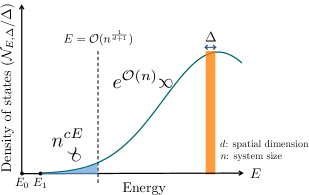
Figure 1: (color online). We suppose a scaling of $n^{\mathcal{O}(E)}$ for the density of states, which typically appears in non-critical (or gapped) systems at low temperatures. Subsequently, under the assumption of clustering (Def. 1) of a canonical state, all the low-lying eigenstates are proved to demonstrate the same properties as those of the ground state (blue shaded). In high-energy regime, the weak version of the ETH and the ensemble equivalence between the microcanonical and canonical distributions hold as long as an energy width of $\exp[-\mathcal{O}(n^{\frac{1}{d+1}})]$ is assumed.

In this work, we discuss the eigenstate thermalization in the low-energy regime as well as the high-energy regime, focusing on the system class that satisfies the clustering property (i.e., exponential decay of bi-partite correlations, see Def. 1 below). The clustering property is one of the most general thermodynamic properties in noncritical systems, valid irrespective of characteristics such as the nonintegrability, energy regime, and so on. In this paper, a special attention is paid on the difference in the density of states between the low and high energy regimes, as the density of states can vary with respect to the energy regime (See Fig. 1). We show that the clustering property is deeply connected to several properties on the eigenstate thermalization through the density of states.

To study the low-energy regime, we consider a system having density of states with a power-law dependence on the system size, typically observed in gapped systems Hastings (2007); Brandão and Cramer (2015); Masanes (2009). Note that the gapped systems satisfy the clustering property even for the ground state. Then, we report that the eigenstate thermalization is proven for low-lying energy eigenstates near the ground state. This implies that low-lying eigenstates behave similar to the ground state in the sense that these yield the same expectation values for local observables. This can also be considered as zero-temperature version of eigenstate thermalization. In the high-energy regime, we discuss the ensemble equivalence between microcanonical and canonical ensemble. We show that it holds for sub-exponentially small energy width with respect to the system size, i.e., $\Delta_{c}\sim\exp[-\mathcal{O}(n^{\frac{1}{d+1}})]$, thus achieving an exponential improvement compared to the recent results in Brandao and Cramer (2015); Tasaki (2018). Although this small energy width cannot reach the ETH since the energy spacing is even smaller, we quantitatively discuss the weak version of the eigenstate thermalization. It implies that the variance of the deviation from the ETH decays as the system size increases. We show that the decaying rate depends on $(\log n)^{d+1}/n$, where $n$ and $d$ are the system size and the spatial dimension, respectively. This is consistent with the recent numerical observations Alba (2015).

Setup of Hamiltonian.— For simplicity, we consider a (1/2)-quantum spin system defined on a $d$-dimensional hypercubic lattice. The present analysis is applied to generic quantum spin numbers and lattice structures. The Hamiltonian comprises $n$ local terms:

$$H=\sum_{i=1}^{n}H_{i},\quad\|H_{i}\|\leq g$$ (1)

where $\|\cdot\|$ represents the operator norm. By taking the energy unit appropriately, we set $g=1$. The local Hamiltonian, $H_{i}$, contains spin operators that act on spins, $j$, with distance, ${\rm dist}(i,j)\leq\ell_{0}$, where ${\rm dist}(i,j)$ is the Manhattan distance. Notably, translation invariance of the Hamiltonian is not assumed here. Subsequently, without loss of generality, we set the energy of the ground state to zero. In addition, we assume that the system satisfies the clustering property for the canonical distribution that is defined as follows:

Definition 1.

Let $\rho_{\beta}$ be a canonical distribution with an inverse temperature, $\beta$,

$$\rho_{\beta} :=e^{-\beta H}/Z_{\beta},$$ (2)

where $Z_{\beta}$ is the partition function. Let $A_{X},B_{Y}$ be the arbitrary operators supported on subsets $X$ and $Y$, respectively. A density matrix $\rho_{\beta}$ is assumed to satisfy the $(r,\xi)$-clustering if the following condition is satisfied,

$$\left|\langle A_{X}B_{Y}\rangle_{\beta}-\langle A_{X}\rangle_{\beta}\langle B_{Y}\rangle_{\beta}\right|\leq\|A_{X}\|\|B_{Y}\|e^{-{\rm dist}(X,Y)/\xi}$$

for ${\rm dist}(X,Y)\geq r$ with fixed constants, $r$ and $\xi$. Here, ${\rm dist}(X,Y)=\min_{i\in X,j\in Y}{\rm dist}(i,j)$ and $\langle...\rangle_{\beta}={\rm tr}(...\rho_{\beta})$.

So far, several previous rigorous studies have addressed the clustering property for low and high energy regimes Araki (1969); Hernández-Santana et al. (2015); Park and Yoo (1995); Ueltschi (2004); Kliesch et al. (2014); Fröhlich and Ueltschi (2015); Kuwahara et al. (2019); Thomas and Yin (1983); Kennedy (1985); Takahashi (1986); Winterfeldt and Ihle (1997). The clustering property is thought to be a rather generic phenomenon in non-critical many-body quantum systems. Note that no direct connection exists between the clustering property and the nonintegrability of the system; hence, even integrable systems can exhibit clustering.

Definition of the eigenstate thermalization.— We consider the macroscopic observable, $\Omega$, that is composed solely of local operators:

$$\Omega =\sum_{i=1}^{n}\Omega_{i},\quad\|\Omega_{i}\|\leq 1,$$ (3)

where $\Omega_{i}$ is composed of spin operators that act on spins, $j$, with distance, ${\rm dist}(i,j)\leq\ell$. Throughout this paper, we set $\ell\geq r$. Using these observables, we define the eigenstate thermalization irrespective of the energy regime. Let $|E_{m}\rangle$ and $E_{m}$ be the $m$th eigenstate and the eigenenergy of the system, respectively ($m=0,\ldots,2^{n}-1$). For the macroscopic observable, the eigenstate thermalization is defined as

$$|\langle E_{m}|(\Omega/n)|E_{m}\rangle-\langle\Omega/n\rangle_{\beta}|\to 0,\quad n\to\infty\,,$$ (4)

for all energy eigenstates within a given finite energy shell. The canonical average is computed with the temperature corresponding to the energy. The eigenstate thermalization here is defined as the ensemble equivalence between the single eigenstate and the canonical ensemble in terms of the given observables Sup .

In case that one can not access the eigenstate thermalization described above, we consider the weak version of eigenstate thermalization to quantify ETH-like properties for general classes of systems including integrable systems Biroli et al. (2010); Iyoda et al. (2017). To this end, we define the microcanonical distribution in the energy shell with the energy width $\Delta$:

$$\rho_{{E},\Delta} :={\cal N}_{{E},\Delta}^{-1}\sum_{E_{m}\in({E}-\Delta,{E}]}|E_{m}\rangle\langle E_{m}|,$$ (5)

where ${\cal N}_{{E},\Delta}$ is the number of eigenstates within the energy shell. Hence, ${\cal N}_{{E},\Delta}/\Delta$ is the density of states depicted in Fig. 1. Then, the weak version of eigenstate thermalization is written as

$${\rm Var}_{{E},\Delta}(\Omega/n) \to 0\,,~{}~{}~{}~{}~{}~{}~{}~{}n\to\infty\,,$$ (6)

$${\rm Var}_{{E},\Delta}(O) :=\!\!\!\!\!\!\!\!\sum_{E_{m}\in({E}-\Delta,{E}]}\!\!\!\!\!\frac{\left(\langle E_{m}|O|E_{m}\rangle-\langle O\rangle_{{E},\Delta}\right)^{2}}{{\cal N}_{{E},\Delta}},$$ (7)

where $\langle O\rangle_{{E},\Delta}$ is the microcanonical average for an arbitrary operator $O$.

Results for low-energy regime.— We derive the following theorem, by which we can prove the eigenstate thermalization in the low energy regime if the density of states is sparse, as depicted in Fig. 1. The clustering property leads to the Chernoff-Hoeffding-type concentration inequality for macroscopic observables  Kuwahara (2016a); Anshu (2016), which is crucial in the derivation. We provide the details of the derivation in the supplementary material Sup .

Theorem 1.

Let $\beta^{\ast}$ be an arbitrary inverse temperature for which the canonical ensemble, $\rho_{\beta^{\ast}}$, satisfies $(r,\xi)$-clustering. Then, any energy eigenstate, $|E_{m}\rangle$, satisfies

$$|\langle E_{m}|(\Omega/n)|E_{m}\rangle\!-\!\langle\Omega/n\rangle_{\infty}| \!\leq\!(1/\sqrt{n})\max(c_{1}{\cal A}_{1},c_{2}{\cal A}_{2}),$$

$${\cal A}_{1}= \left[\beta^{\ast}E_{m}+\log Z_{\beta^{\ast}}\right]^{(d+1)/2}\!\!,$$ (8)

$${\cal A}_{2}= \left[\ell^{d}(\beta^{\ast}E_{m}+\log Z_{\beta^{\ast}})\right]^{1/2}\!,$$

where $\langle\cdots\rangle_{\infty}$ is the average in the ground state and the constants $c_{1},c_{2}$ depend on $d,r,\xi$, and $\ell_{0}$.

As we have set the energy of the ground state to zero, the quantity $\log Z_{\beta^{\ast}}$ always has a positive value ft (2). We emphasize that even in the presence of degeneracy, the theorem is valid for an arbitrary superposition of degenerate eigenstates.

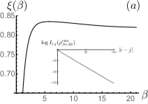
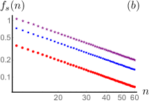
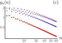
Figure 2: (color online) Numerical demonstrations. The first figure (a) shows $\beta$-dependence of the correlation length, $\xi(\beta)$, in the canonical state $\rho_{\beta}$ ($h=3/2$). We calculate the mutual information for the spin pairs of $\{r,n-r+1\}_{r=1}^{n/2}$ with $n=100$. In order to determine the correlation length, $\xi(\beta)$, we fit $\log[I_{i,j}(\rho_{\beta})]$ with respect to $|i-j|$ by a linear function using the least squares method. The second and third figures (b) and (c) show the log–log plots of the system-size dependence of the functions, $f_{s}(n)$ and $g_{s}(n)$. In the plots, points represented by circle ($\bullet$), square ($\blacksquare$), and star ($\star$) correspond to the cases of $s=3$, $s=5$, and $s=7$, respectively. For $s=7$, the behavior of $f_{s}(n)$ and $g_{s}(n)$ for a large $n$ are estimated by $n^{-0.998}$ and $n^{-0.854}$, respectively.

If we consider the system that shows $\log Z_{\beta^{\ast}}\sim\mathcal{O}(1)$ ft (3) and, in addition, look at the energy regime $E_{m}\lesssim\mathcal{O}(n^{1/(d+1)})$, the right-hand side vanishes in the thermodynamic limit. This implies the eigenstate thermalization. In other words, these low-lying eigenstates are indistinguishable from the ground state as long as the local observables are measured. A possible realistic situation for obtaining this scenario is given by the systems satisfying the following relation for the density of states in an energy shell $({{E}}-1,{{E}}]$ for the low-energy regime (See Fig.1) Hastings (2007); Brandão and Cramer (2015); Masanes (2009):

$${\cal N}_{{{E}},1} \leq n^{c{{E}}}.$$ (9)

In this case, we can demonstrate that the quantity $\log Z_{\beta^{\ast}}$ with $\beta^{\ast}\propto\log n$ becomes the order of $1$ in the thermodynamic limit ft (4). Behavior of the density of states (9) is ubiquitous especially in the gapped systems as discussed in Refs. Hastings (2007); Brandão and Cramer (2015); Masanes (2009). This behavior is rather general, when low-lying eigenstates are constructed with a superposition of locally excited states. We also demonstrate this with a specific model below. Notably, in the finite-dimensional gapped systems, it has been rigorously proved that the ground state shows an exponential decay for spatially separated observables Hastings and Koma (2006); Nachtergaele and Sims (2006), and hence, it is generally expected that the canonical distribution exhibits the clustering property in an extremely low-energy regime.

As the theorem 1 is derived from the clustering property, the scenario described here should be satisfied irrespective of the (non)integrability. This is quite different from the eigenstate thermalization observed in the high-energy regime, which generally requires the nonintegrability of the Hamiltonian.

Numerical demonstration on the eigenstate thermalization .— To obtain a better understanding of the realization of eigenstate thermalization, we consider a simple integrable model. Let us consider the $xy$ model with a magnetic field:

$$H=\sum_{i=1}^{n-1}[(3/4)\sigma_{i}^{x}\sigma_{i+1}^{x}+(1/4)\sigma_{i}^{y}\sigma_{i+1}^{y}]+h\sum_{i=1}^{n}\sigma_{i}^{z},$$ (10)

where $\sigma_{i}^{\alpha}\,(\alpha=x,y,z)$ is the $\alpha$-component of the Pauli matrix at the site $i$. We consider the gapped case with $h>1$. The Hamiltonian is diagonalized into the Fermionic representation Chung and Peschel (2001); Lieb et al. (1961), $H=\sum_{k=1}^{n}2\epsilon_{k}c_{k}^{\dagger}c_{k}$, where $\epsilon_{k}$ is a positive eigenmode energy for the $k$th mode and $c_{k}^{\dagger}$ is the creation operator (we adjust the energy of the ground state to zero). An arbitrary eigenstate is expressed as

$$|E_{m}\rangle =\prod_{k=1}^{n}[c_{k}^{\dagger}]^{q_{k}}|0\rangle\quad q_{k}=0\quad{\rm or}\quad 1,$$ (11)

where $|0\rangle$ is the vacuum state and $m$ is determined by the choice of $\{q_{k}\}_{k=1}^{n}$. In this representation, the ground state is identical to the vacuum state. For $h>1$, each eigenmode energy, $\epsilon_{k}$, is of the order $1$. Hence, the number of eigenstates can be estimated through a simple combinatorial argument ftc , which justifies the relation (9).

We here verify the clustering property in the present model. We consider the mutual information between two separated spins for $h=3/2$. For a given density matrix $\rho$, the mutual information $I_{i,j}(\rho)$ between the sites $i$ and $j$ is defined as, $I_{i,j}(\rho)=S(\rho_{i})+S(\rho_{j})-S(\rho_{i,j})$, where $S(\rho^{\prime})$ is the Von Neumann entropy of the density matrix $\rho^{\prime}$; and $\rho_{i}$ and $\rho_{i,j}$ are reduced density matrices of a single site, $i$, and two sites $i,j$, respectively. We first verify that $I_{i,j}(\rho_{\beta})$ shows an exponential decay as a function of distance $|i-j|$, which is demonstrated in the inset of Fig. 2 (a). We calculate the $\beta$-dependence of the correlation length $\xi(\beta)$ and present a plot in the primary graph of Fig. 2 (a). This plot indicates the clustering property even for extremely low-temperatures.

From the clustering property and the energy dependence of the number of states (9), the emergence of the eigenstate thermalization can be directly observed. Let $\mathcal{E}_{s}$ be the set of all the eigenstates (11) with $\sum_{k=1}^{n}q_{k}\leq s$. The set includes low-lying excited states whose energy is of the order $1$. Hence, we consider a deviation from the local thermodynamic property for the eigenstates in the $\mathcal{E}_{s}$ set and the ground state. We define the follwoing two quantities:

$$f_{s}(n) :=\max_{|E_{m}\rangle\in\mathcal{E}_{s}}(1/n)|\langle E_{m}|\hat{M}_{z}|E_{m}\rangle-\langle E_{0}|\hat{M}_{z}|E_{0}\rangle|\,,$$

$$g_{s}(n) :=\max_{|E_{m}\rangle\in\mathcal{E}_{s}}\bigl{\|}\rho^{[m]}_{i_{0},i_{0}+1}-\rho^{[0]}_{i_{0},i_{0}+1}\bigr{\|}_{1}\,,$$ (12)

where we use magnetization as a local observable, i.e., $\hat{M}_{z}=\sum_{i=1}^{n}\sigma_{i}^{z}$, and $i_{0}=\lfloor n/2\rfloor$. The matrices $\rho^{[m]}_{i_{0},i_{0}+1}$ and $\rho^{[0]}_{i_{0},i_{0}+1}$ are the reduced density matrices at the sites $\{i_{0},i_{0}+1\}$ of the density matrix $|E_{m}\rangle\langle E_{m}|$ and the ground state $|E_{0}\rangle\langle E_{0}|$, respectively. The quantities $f_{s}(n)$ and $g_{s}(n)$ measure the deviation in terms of local observable (magnetization) and the reduced density matrices, respectively, between eigenstates in the set $\mathcal{E}_{s}$ and the ground state. In Fig. 2 (b) and (c), we show $f_{s}(n)$ and $g_{s}(n)$ for $s=3,5,7$ as a function of the system size, $n$. The figures show the systematic decay of these quantities as the system size increases. This is a direct and clear indication of the emergence of eigenstate thermalization. The decay rate in this specific case is indeed faster by a factor of $n^{-1/2}$ compared to the decay rate obtained from the theorem 1.

Results in the high-energy regime.— As the clustering property is satisfied even in integrable systems, the eigenstate thermalization defined in Eq. (4) should not be derived for the high energy regime, where the density of states is exponentially large with respect to the system size as depicted in Fig. 1. Instead, we prove the weak version of eigenstate thermalization.

We first derive a theorem on the ensemble equivalence between microcanonical and canonical ensembles, which shows that the ensemble equivalence holds with a small energy width, while it also shows that the eigenstate thermalization cannot be achieved in the high energy regime only from the clustering property. The theorem is given as follows.

Theorem 2.

Let us consider the energy shell, $({E}-\Delta,{E}]$ and the inverse temperature, $\beta$ that maximizes $e^{-\beta{E}}{\cal N}_{{E},\Delta}$ Tasaki (2018). If the canonical ensemble, $\rho_{\beta}$, satisfies the $(r,\xi)$-clustering, the microcanonical ensemble, $\rho_{{E},\Delta}$, satisfies the following:

$$\left|\langle\Omega/n\rangle_{{E},\Delta}-\langle\Omega/n\rangle_{\beta}\right| \leq(1/\sqrt{n})\max(c^{\prime}_{1}{\cal B}_{1},c^{\prime}_{2}{\cal B}_{2}),$$

$${\cal B}_{1} =\left[\log(\sqrt{n}/\Delta)\right]^{(d+1)/2},$$ (13)

$${\cal B}_{2} =\left[\ell^{d}\log(\sqrt{n}/\Delta)\right]^{1/2},$$

where $\langle\Omega\rangle_{\beta}$ is the average with respect to the corresponding canonical ensembles, and the constants $c^{\prime}_{1}$, $c^{\prime}_{2}$ depend on $d$, $r$, $\xi$, and $\ell_{0}$.

Based on the theorem, we can estimate a minimum value to justify the ensemble equivalence for the large system size. To obtain $\langle\Omega/n\rangle_{{E},\Delta}\approx\langle\Omega/n\rangle_{\beta}$ for $n\to\infty$, we need to impose ${\cal B}_{1,2}\lesssim\mathcal{O}(n^{1/2})$ from (13). This condition gives the lower bound on the energy width, $\Delta_{c}$, for the ensemble equivalence as ft (1)

$$\Delta_{c} \sim\exp\left[-\mathcal{O}(n^{1/(d+1)})\right].$$ (14)

This implies that even a subexponentially small energy width is sufficient to guarantee the ensemble equivalence. Although studies on the ensemble equivalence has a long history Lima (1972, 1971); De Roeck et al. (2006); Müller et al. (2015); Georgii (1995); Touchette (2011, 2015), the finite-size effect has been studied quite recently Brandao and Cramer (2015); Tasaki (2018). Our system-size dependence is an exponential improvement from the state-of-the-art estimation $\mathcal{O}(n^{-1/2})$ in Tasaki (2018). However, even this energy width cannot discriminate a single eigenstate in the high energy regime having exponentially high density of states with respect to the system size, and hence one cannot reach the eigenstate thermalization.

We next show that the weak version of the eigenstate thermalization can be quantitatively argued Biroli et al. (2010); Iyoda et al. (2017). As defined in (6), the weak version of eigenstate thermalization states that almost all the eigenstates in the energy shell have the same property. Using the variance, ${\rm Var}_{{E},\Delta}(\Omega/n)$, defined in Eq. (7), we can derive the following finite-size effect (see Sec. III in Sup ):

$${\rm Var}_{{E},\Delta}(\Omega/n) \leq(1/n)\max(c^{\prime\prime}_{1}{\cal B}_{1}^{2},c^{\prime\prime}_{2}{\cal B}_{2}^{2})\,,$$ (15)

where ${\cal B}_{1},{\cal B}_{2}$ were defined in Eq. (13), and $c_{1}^{\prime\prime}$, $c_{2}^{\prime\prime}$ are constants that depend on $d$, $r$, $\xi$, and $\ell_{0}$. The inequality (15) implies that by taking the energy width $\Delta=1/{\rm poly}(n)$, the following holds

$${\rm Var}_{{E},\Delta}(\Omega/n) \lesssim\log^{d+1}(n)/n\,.$$ (16)

It is noteworthy that recent calculations by Alba Alba (2015) showed an example that expresses the variance of $\mathcal{O}(1/n)$. This indicates that our estimation (16) is the best general upper bound on the weak ETH up to a logarithmic correction.

Summary and discussion.— Theorem 1 gives a clear scenario for achieving the eigenstate thermalization in low-lying eigenstates near the ground state, irrespective of the (non)integrability of the Hamiltonian. This is quite different from the eigenstate thermalization in the high-energy regime where the nonintegrability is assumed to be a key-ingredient Rigol et al. (2007); Calabrese et al. (2011). We also emphasize that the ETH can be argued at the level of reduced density matrix for local sites, which is presented in Sec. VI in Sup . Moreover, our approach on ensemble equivalence can be extended to a wider class of systems for e.g., long-range interacting systems where the Chernoff-Hoeffding type concentration bound still holds Kuwahara (2016b); Kuwahara et al. (2017); Kuwahara and Saito (2019)

We comment on the relation between the present argument and the many-body localization phenomenon Nandkishore and Huse (2015), where the ETH is violated. In the present analysis, we consider sufficiently low-energy regime, $\beta^{\ast}\propto\log n$. Although the one-dimensional systems exhibit the clustering property in general Araki (1969), it is justified only for $\beta\lesssim\mathcal{O}(1)$. In systems with many-body localization, the canonical state $\rho_{\beta}$ does not satisfy the clustering property for $\beta^{\ast}\propto\log n$. We have discussed this point in Sec. VI of Sup with a numerical calculation. We stress that Theorem 1 has no inconsistency with the absence of thermalization in systems with many-body localization.

I Setup

I.1 Notations and definitions

We iterate several definitions that are presented in the primary text. The Hamiltonian that we considered consists of $n$ local terms:

$$H=\sum_{i=1}^{n}H_{i}\,,\quad\|H_{i}\|\leq 1.$$ (S.1)

The local Hamiltonian $H_{i}$ contains spin operators that act nontrivially on spins $j$ with the distance ${\rm dist}(i,j)\leq\ell_{0}$.

The canonical and microcanonical distributions are defined as

$$\rho_{\beta} :={e^{-\beta H}\over Z_{\beta}}\,,$$ (S.2)

$$\rho_{{{E}},\Delta} :={1\over{\cal N}_{{{E}},\Delta}}\sum_{E_{m}\in({{E}}-\Delta,{{E}}]}|E_{m}\rangle\langle E_{m}|\,,$$ (S.3)

where $Z_{\beta}$ is the partition function $Z_{\beta}={\rm tr}e^{-\beta H}$, and $|E_{m}\rangle$ is the $m$th eigenstate of the Hamiltonian ($m=0,1,\ldots,2^{n}-1$) and we define

$${\cal N}_{{{E}},\Delta} :={\rm tr}\left[\sum_{E_{m}\in({{E}}-\Delta,{{E}}]}|E_{m}\rangle\langle E_{m}|\right]\,.$$ (S.4)

For an arbitrary operator $O$, the canonical and microcanonical averages are expressed as follows, respectively:

$$\langle O\rangle_{\beta} :={\rm tr}(\rho_{\beta}O)\,,$$ (S.5)

$$\langle O\rangle_{{{E}},\Delta} :={\rm tr}(\rho_{{{E}},\Delta}O)\,.$$ (S.6)

Next, we focus on the following operator:

$$\Omega=\sum_{i=1}^{n}\Omega_{i},\quad\|\Omega_{i}\|\leq 1,$$ (S.7)

where $\Omega_{i}$ is composed of spin operators that act on spins $j$ with the distance ${\rm dist}(i,j)\leq\ell$.

In our theory, we assume the clustering property for $\rho_{\beta}$, which is defined as follows:

Definition 2.

Let $A_{X},B_{Y}$ be arbitrary operators supported on subsets $X$ and $Y$, respectively. We say that a density matrix $\rho$ satisfies the $(r,\xi)$-clustering if

$$\left|{\rm tr}(\rho A_{X}B_{Y})-{\rm tr}(\rho A_{X}){\rm tr}(\rho B_{Y})\right|\leq\|A_{X}\|\|B_{Y}\|e^{-{\rm dist}(X,Y)/\xi}$$

for ${\rm dist}(X,Y)\geq r$, where $r$ and $\xi$ are fixed constants.

I.2 On the definition of eigenstate thermalization and ensemble equivalence

We start with the established definition on ensemble equivalence. Suppose that we have two ensembles $\rho_{A}$ and $\rho_{B}$. We say that the ensemble equivalence holds between these ensembles in terms of the observable $O$, if the following is satisfied

$${\rm Tr}(\rho_{A}O)-{\rm Tr}(\rho_{B}O) =0\,.$$ (S.8)

Examples include the ensemble equivalence for the canonical ensemble $\rho_{\beta}$ and the microcanonical ensemble $\rho_{E,\Delta}$ as we address in this paper. Another example is the equivalence between the canonical ensemble for a many-particles system and the Gibbs ensemble. In this paper, we are interested in the local observable $\Omega/n$. Then, the ensemble equivalence between $\rho_{\beta}$ and $\rho_{E,\Delta}$ holds if the following is satisfied

$${\rm Tr}(\rho_{E,\Delta}(\Omega/n))-{\rm Tr}(\rho_{\beta}(\Omega/n)) =0\,.$$ (S.9)

As an extreme case, we consider very small energy window so that the energy shell contains a single eigenstate $|E_{m}\rangle$. In this case, the microcanonical ensemble is replaced by $|E_{m}\rangle\langle E_{m}|$ leading to

$${\rm Tr}(|E_{m}\rangle\langle E_{m}|(\Omega/n))-{\rm Tr}(\rho_{\beta}(\Omega/n)) =0\,.$$ (S.10)

This is the eigenstate thermalization meaning that the single eigenstate is equivalent to the canonical ensemble in terms of the local observable.

I.3 Concentration inequality

As the core of the proof of our theorems, we utilize the following concentration inequality that is resulted from the $(r,\xi)$-clustering. We start with the following lemma, whose proof is shown in Section VII. This lemma is essentially the same as that in Ref. Anshu (2016).

Lemma 1.

Let $\rho$ be an arbitrary density matrix that satisfies the $(r,\xi)$-clustering (Def. 2). Subsequently, for an arbitrary even integer $M$, the $M$-th moment of the operator $\Omega$ is bounded from above by

$${\rm tr}\Bigl{[}\bigl{(}\Omega-\langle\Omega\rangle_{\rho}\bigr{)}^{M}\rho\Bigr{]} \leq[8\alpha Mn(3\ell)^{d}]^{M/2}+3\xi[8\alpha nM^{d+1}(3\xi d/2)^{d}]^{M/2}$$

$$=:3\xi[\tilde{c}_{1}nM^{d+1}/(2e)]^{M/2}+[\tilde{c}_{2}\ell^{d}Mn/(2e)]^{M/2}$$ (S.11)

with $\langle\cdots\rangle_{\rho}:={\rm tr}(\rho\cdots)$ and

$$\tilde{c}_{1}:=16e\alpha(3\xi d/2)^{d}\quad{\rm and}\quad\tilde{c}_{2}:=3^{d}(16e\alpha),$$ (S.12)

where $\alpha$ is a geometric parameter defined in Ineq. (S.69) of Section VII, and we assume $\ell\geq r$. If $\ell\leq r$, the parameter $\ell$ in (S.11) is replaced by $r$.

We define the probability density to observe the value $x$ for the observable $\Omega$ in terms of the density matrix $\rho$

$$P_{\rho}(x) :={\rm tr}\left[\rho\delta(x-\Omega)\right]\,,$$ (S.13)

where $\delta(\cdots)$ is the Dirac delta function. We relate the inequality (S.11) to the concentration bound for this distribution. For the given positive value $x_{0}$, the following relation for the cumulative distribution is satisfied:

$$P_{\rho}(|x-\langle\Omega\rangle_{\rho}|\geq x_{0}):=\int_{|x-\langle\Omega\rangle_{\rho}|\geq x_{0}}P_{\rho}(x)dx =P_{\rho}((x-\langle\Omega\rangle_{\rho})^{M}\geq x_{0}^{M})$$

$$\leq{{\rm tr}\left[\rho(x-\langle\Omega\rangle_{\rho})^{M}\right]\over x_{0}^{M}}$$

$$\leq 3\xi\left(\frac{\tilde{c}_{1}nM^{d+1}}{2ex_{0}^{2}}\right)^{M/2}+\left(\frac{\tilde{c}_{2}\ell^{d}Mn}{2ex_{0}^{2}}\right)^{M/2}\,,$$ (S.14)

where $M$ is a positive even integer. We use the Markov inequality for the second line, and the inequality (S.11) for the third line. We subsequently choose $M/2$ ($\in\mathbb{Z}$) as

$$\frac{M}{2}=\left\lfloor\min\left\{\left(\frac{x_{0}^{2}}{\tilde{c}_{1}n}\right)^{1/(d+1)},~{}\frac{x_{0}^{2}}{\tilde{c}_{2}\ell^{d}n}\right\}\right\rfloor,$$ (S.15)

where $\lfloor\cdots\rfloor$ is the floor function. This choice ensures $\frac{\tilde{c}_{1}nM^{d+1}}{2ex_{0}^{2}}\leq 1/e$ and $\frac{\tilde{c}_{2}\ell^{d}Mn}{2ex_{0}^{2}}\leq 1/e$; hence, the upper bound (S.14) reduces to

$$P_{\rho}(|x-\langle\Omega\rangle_{\rho}|\geq x_{0}) \leq(e+3e\xi)\max\left(e^{-[x_{0}^{2}/(\tilde{c}_{1}n)]^{1/(d+1)}},e^{-x_{0}^{2}/(\tilde{c}_{2}\ell^{d}n)}\right)\,.$$ (S.16)

Note that the cumulative distribution must be less than $1$. Combining this with the inequality above, we obtain the following relation:

$$P_{\rho}(|x-\langle\Omega\rangle_{\rho}|\geq x_{0}) \leq\min\left[1,(e+3e\xi)\max\left(e^{-[x_{0}^{2}/(\tilde{c}_{1}n)]^{1/(d+1)}},e^{-x_{0}^{2}/(\tilde{c}_{2}\ell^{d}n)}\right)\right].$$ (S.17)

I.4 Useful formula

For the calculations in the following sections, the following lemma is useful.

Lemma 2.

Let $p(x)$ be an arbitrary probability distribution whose cumulative distribution is bounded from above:

$$P(|x-a|\geq x_{0}):=\int_{|x-a|\geq x_{0}}p(x)dx\leq\min(1,e^{-x_{0}^{\gamma}/\sigma+x_{1}})\,,~{}~{}~{}~{}~{}\gamma>0,~{}\sigma>0,~{}x_{0}>0\,.$$ (S.18)

Subsequently, for an arbitrary $k\in\mathbb{N}$, we obtain

$$\int_{-\infty}^{\infty}|x-a|^{k}p(x)dx\leq(2\sigma x_{1})^{k/\gamma}+\frac{k}{\gamma}(2\sigma)^{k/\gamma}\Gamma(k/\gamma)$$ (S.19)

with $\Gamma(\cdot)$ as the gamma function.

I.4.1 Proof of Lemma 2

We first define $\tilde{x}:=(2\sigma x_{1})^{1/\gamma}$, which is the solution of $-\tilde{x}^{\gamma}/\sigma+x_{1}=-\tilde{x}^{\gamma}/(2\sigma)$. Subsequently, $-x_{0}^{\gamma}/\sigma+x_{1}\leq-x_{0}^{\gamma}/(2\sigma)$ for $x_{0}\geq\tilde{x}$; that is, $P(|x-a|\geq x_{0})\leq e^{-x_{0}^{\gamma}/(2\sigma)}$ for $x_{0}\geq\tilde{x}$. Using this, we obtain the following relation:

$$\int_{-\infty}^{\infty}|x-a|^{k}p(x)dx=\int_{-\infty}^{\infty}|x|^{k}p(x+a)dx \leq\tilde{x}^{k}\int_{-\tilde{x}}^{\tilde{x}}p(x+a)dx+\int_{x\geq\tilde{x}}x^{k}[p(x+a)+p(-x+a)]dx$$

$$\leq\tilde{x}^{k}-\int_{\tilde{x}}^{\infty}x^{k}\frac{d}{dx}\left[\int_{|x^{\prime}-a|\geq x}p(x^{\prime})dx^{\prime}\right]dx.$$ (S.20)

The second term reduces to

$$-\int_{\tilde{x}}^{\infty}x^{k}\frac{d}{dx}\left[\int_{|x^{\prime}-a|\geq x}p(x^{\prime})dx^{\prime}\right]dx =-\tilde{x}^{k}P(|x-a|\geq\tilde{x})+\int_{\tilde{x}}^{\infty}kx^{k-1}\left[\int_{|x^{\prime}-a|\geq x}p(x^{\prime})dx^{\prime}\right]dx$$

$$\leq\int_{0}^{\infty}kx^{k-1}e^{-x^{\gamma}/(2\sigma)}dx=\frac{k}{\gamma}(2\sigma)^{k/\gamma}\Gamma(k/\gamma),$$ (S.21)

where we use the partial integration in the first equation. By combining the two inequalities (S.20) and (S.21), we obtain the inequality (S.19). This completes the proof. $\square$

II Proof of Theorem 1 in the main text.

In this section, we prove Theorem 1 . We start by defining the probability distribution to observe the value $x$ for the observable $\Omega$ for a given eigenstate $|E_{m}\rangle$:

$$P_{E_{m}}(x) ={\rm tr}\left[\,|E_{m}\rangle\langle E_{m}|\,\delta(x-\Omega)\,\right]\,.$$ (S.22)

Subsequently, we consider the cumulative distribution $P_{E_{m}}(|x-\langle\Omega\rangle_{\beta^{\ast}}|\geq x_{0})$ where, at this stage, the inverse temperature $\beta^{\ast}$ is arbitrary. From Markov’s inequality with a positive even integer $M$, we have the following relation:

$$P_{E_{m}}(|x-\langle\Omega\rangle_{\beta^{\ast}}|\geq x_{0}) =P_{E_{m}}((x-\langle\Omega\rangle_{\beta^{\ast}})^{M}\geq x_{0}^{M})$$

$$\leq{\langle E_{m}|(\Omega-\langle\Omega\rangle_{\beta^{\ast}})^{M}|E_{m}\rangle\over x_{0}^{M}}\,.$$ (S.23)

Below, we bound $\langle E_{m}|(\Omega-\langle\Omega\rangle_{\beta^{\ast}})^{M}|E_{m}\rangle$ from above using $\langle(\Omega-\langle\Omega\rangle_{\beta^{\ast}})^{M}\rangle_{\beta^{\ast}}$. For notational convenience, we define $E_{\beta^{\ast}}:=-(1/\beta^{\ast})\ln Z_{\beta^{\ast}}$. Note that the operator $(\Omega-\langle\Omega\rangle_{\beta^{\ast}})^{M}$ is a non-negative operator; hence, we can obtain the following relation:

$$\langle E_{m}|(\Omega-\langle\Omega\rangle_{\beta^{\ast}})^{M}|E_{m}\rangle =e^{\beta^{\ast}E_{m}}e^{-\beta^{\ast}E_{m}}\langle E_{m}|(\Omega-\langle\Omega\rangle_{\beta^{\ast}})^{M}|E_{m}\rangle$$

$$\leq Z_{\beta^{\ast}}e^{\beta^{\ast}E_{m}}\sum_{E_{m^{\prime}}\in(-\infty,\infty)}{e^{-\beta^{\ast}E_{m^{\prime}}}\over Z_{\beta^{\ast}}}\langle E_{m^{\prime}}|(\Omega-\langle\Omega\rangle_{\beta^{\ast}})^{M}|E_{m^{\prime}}\rangle$$

$$=e^{\beta^{\ast}(E_{m}-E_{\beta^{\ast}})}\langle(\Omega-\langle\Omega\rangle_{\beta^{\ast}})^{M}\rangle_{\beta^{\ast}}\,.$$ (S.24)

Combining the inequality (S.23) with this, the following relation is obtained:

$$P_{E_{m}}(|x-\langle\Omega\rangle_{\beta^{\ast}}|\geq x_{0}) \leq\,e^{\beta^{\ast}(E_{m}-E_{\beta^{\ast}})}{\langle(\Omega-\langle\Omega\rangle_{\beta^{\ast}})^{M}\rangle_{\beta^{\ast}}\over x_{0}^{M}}\,.$$ (S.25)

From the assumption of the ($r$,$\xi$)-clustering for the density matrix $\rho_{\beta^{\ast}}$, the $M$-th moment $\langle(x-\langle\Omega\rangle_{\beta^{\ast}})^{M}\rangle_{\beta^{\ast}}$ obeys the inequality (S.11) from Lemma 1. Hence, we have

$$P_{E_{m}}(|x-\langle\Omega\rangle_{\beta^{\ast}}|\geq x_{0}) \leq e^{\beta^{\ast}(E_{m}-E_{\beta^{\ast}})}\left[3\xi\left(\frac{\tilde{c}_{1}nM^{d+1}}{2ex_{0}^{2}}\right)^{M/2}+\left(\frac{\tilde{c}_{2}\ell^{d}Mn}{2ex_{0}^{2}}\right)^{M/2}\right]\,.$$ (S.26)

By choosing $M$ as in Eq. (S.15), we arrive at the concentration bound as

$$P_{E_{m}}(|x-\langle\Omega\rangle_{\beta^{\ast}}|\geq x_{0})\leq\min\left\{1,\,e^{\beta^{\ast}(E_{m}-E_{\beta^{\ast}})}(e+3e\xi)\max\left(e^{-[x_{0}^{2}/(\tilde{c}_{1}n)]^{1/(d+1)}},e^{-x_{0}^{2}/(\tilde{c}_{2}n)}\right)\right\}.$$ (S.27)

Having obtained the concentration inequality, we evaluate the integration bound:

$$|\langle E_{m}|\Omega|E_{m}\rangle-\langle\Omega\rangle_{\beta^{\ast}}| =\left|\int_{-\infty}^{\infty}(x-\langle\Omega\rangle_{\beta^{\ast}})P_{E_{m}}(x)dx\right|\leq\int_{-\infty}^{\infty}|x-\langle\Omega\rangle_{\beta^{\ast}}|P_{E_{m}}(x)dx\,.$$ (S.28)

For evaluating the most right expression in (S.28), we use Lemma 2 with $k=1$. From the inequality given in (S.27), the parameter sets in Lemma 2 are identified as

$$a =\langle\Omega\rangle_{\beta^{\ast}}\,,$$

$$\{\gamma,\sigma,x_{1}\} =\{2/(d+1),(\tilde{c}_{1}n)^{\frac{1}{d+1}},\beta^{\ast}(E_{m}-E_{\beta^{\ast}})+\log(e+3e\xi)\}\,\quad{\rm and}\quad\{2,\tilde{c}_{2}\ell^{d}n,\beta^{\ast}(E_{m}-E_{\beta^{\ast}})+\log(e+3e\xi)\}.$$

We subsequently obtain the following from Ineq (S.19):

$$|\langle\Omega\rangle_{E_{m}}-\langle\Omega\rangle_{\beta^{\ast}}|\leq\max(\tilde{\mathcal{A}}_{1},\tilde{\mathcal{A}}_{2})\,,$$ (S.29)

where

$$\tilde{\mathcal{A}}_{1}:=\sqrt{\tilde{c}_{1}n}\left[2\beta^{\ast}(E_{m}-E_{\beta^{\ast}})+2\log(e+3e\xi)\right]^{\frac{d+1}{2}}+2^{(d-1)/2}(d+1)\sqrt{\tilde{c}_{1}n}\Gamma[(d+1)/2],$$

$$\tilde{\mathcal{A}}_{2}:=\sqrt{2\tilde{c}_{2}\ell^{d}n\left[2\beta^{\ast}(E_{m}-E_{\beta^{\ast}})+2\log(e+3e\xi)\right]}+\frac{1}{2}\sqrt{2\pi\tilde{c}_{2}\ell^{d}n}.$$ (S.30)

Therefore, the upper bound (S.28) reduces to

$${1\over n}|\langle E_{m}|\Omega|E_{m}\rangle-\langle\Omega\rangle_{\beta^{\ast}}|\leq{1\over\sqrt{n}}\max\left(c_{1}[\beta^{\ast}(E_{m}-E_{\beta^{\ast}})]^{(d+1)/2},c_{2}[\ell^{d}\beta^{\ast}(E_{m}-E_{\beta^{\ast}})]^{1/2}\right),$$ (S.31)

where $c_{1},c_{2}$ are constants that only depend on $d$, $\xi$, and $\alpha$. Note that $|\langle E_{m}|\Omega|E_{m}\rangle|=|\langle E_{m}|\Omega|E_{m}\rangle-\langle\Omega\rangle_{\beta^{\ast}}|$ for $\langle\Omega\rangle_{\beta^{\ast}}=0$. This completes the proof of Theorem 1 . $\square$

We remark that the inequality (S.31) also holds for the ground state:

$$\frac{1}{n}|\langle E_{0}|\Omega|E_{0}\rangle-\langle\Omega\rangle_{\beta^{\ast}}|\leq{1\over\sqrt{n}}\max\left(c_{1}[\beta^{\ast}(-E_{\beta^{\ast}})]^{(d+1)/2},c_{2}[\ell^{d}\beta^{\ast}(-E_{\beta^{\ast}})]^{1/2}\right)\,,$$ (S.32)

where $|E_{0}\rangle$ is the ground state. Recall that we set the ground energy equal to zero. By combining the inequalities (S.31) and (S.32) with the triangle inequality, we have

$$\frac{1}{n}|\langle E_{m}|\Omega|E_{m}\rangle-\langle E_{0}|\Omega|E_{0}\rangle| \leq\frac{1}{n}|\langle E_{m}|\Omega|E_{m}\rangle-\langle\Omega\rangle_{\beta^{\ast}}|+\frac{1}{n}|\langle E_{0}|\Omega|E_{0}\rangle-\langle\Omega\rangle_{\beta^{\ast}}|$$

$$\leq{2\over\sqrt{n}}\max\left(c_{1}[\beta^{\ast}(E_{m}-E_{\beta^{\ast}})]^{(d+1)/2},c_{2}[\ell^{d}\beta^{\ast}(E_{m}-E_{\beta^{\ast}})]^{1/2}\right).$$ (S.33)

When the ground states exhibit a $D$-fold degeneracy, we denote the ground states by $\{|E_{m}\rangle\}_{m=0}^{D-1}$ (i.e., $H|E_{m}\rangle=0$ for $j\leq D-1$) and consider

$$\langle\Omega\rangle_{\infty}=\frac{1}{D}\sum_{m=0}^{D-1}\langle E_{m}|\Omega|E_{m}\rangle.$$ (S.34)

We subsequently obtain

$$|\langle\Omega\rangle_{\infty}-\langle\Omega\rangle_{\beta^{\ast}}| =\frac{1}{D}\left|\sum_{m=0}^{D-1}\bigl{(}\langle E_{m}|\Omega|E_{m}\rangle-\langle\Omega\rangle_{\beta^{\ast}}\bigr{)}\right|\leq\frac{1}{D}\sum_{m=0}^{D-1}\left|\langle E_{m}|\Omega|E_{m}\rangle-\langle\Omega\rangle_{\beta^{\ast}}\right|.$$ (S.35)

Therefore, we can derive the same inequality as (S.33) for the degenerate ground states.

III Proof of Theorem 2 in the main text.

The proof is almost similar to that of Theorem 1 . In this section, we first prove the following inequality (S.38) which implies that almost all the eigenstates in the energy shell $({{E}}-\Delta,{{E}}]$ have the same expectation value of $\langle\Omega\rangle_{\beta}$. Then, the inequality (13) in the main text is derived as the corollary.

Here, following Ref. Tasaki (2018), we relate the microcanonical energy ${{E}}$ to the inverse temperature $\beta$ as follows:

$${{E}}=\arg\max_{E\in\mathbb{R}}\left(e^{-\beta E}{\cal N}_{E,\Delta}\right).$$ (S.36)

We define a probability distribution $P_{{{E}},\Delta}(x)$ such that

$$P_{{{E}},\Delta}(x)={1\over{\cal N}_{{{E}},\Delta}}\sum_{E_{m}\in({{E}}-\Delta,{{E}}]}\delta(x-\langle E_{m}|\Omega|E_{m}\rangle)\,,$$ (S.37)

where $\delta$ is the Dirac delta function. Using Lemma 1, we obtain the following proposition (the proof is presented in the two subsequent subsections):

Proposition 3.

Let $P_{{{E}},\Delta}(|x-\langle\Omega\rangle_{\beta}|\geq x_{0})\,(x_{0}>0)$ be the cumulative probability distribution of the distribution $P_{{{E}},\Delta}(x)$. Subsequently, if the canonical distribution with the corresponding inverse temperature $\rho_{\beta}$ exhibits the $(r,\xi)$-clustering property, we have

$$P_{{{E}},\Delta}\left(|x-\langle\Omega\rangle_{\beta}|\geq x_{0}\right)\leq\min\left[1,C_{\Delta}\max\left(e^{-[x_{0}^{2}/(\tilde{c}_{1}n)]^{1/(d+1)}},e^{-x_{0}^{2}/(\tilde{c}_{2}\ell^{d}n)}\right)\right]\,,$$ (S.38)

where $C_{\Delta}:=2e^{\beta\Delta}(e+3e\xi)\left[2+(C_{1}\Delta^{-1}\sqrt{n})\right]$ with $C_{1}$ a constant that depends on $d$, $\alpha$, $\xi$ and $\ell_{0}$.

Theorem 2 is a direct result from this proposition. To show Theorem 2 , we evaluate the upper bound of

$$|\langle\Omega\rangle_{{{E}},\Delta}-\langle\Omega\rangle_{\beta}|=\left|\int_{-\infty}^{\infty}\,(x-\langle\Omega\rangle_{\beta})P_{{{E}},\Delta}(x)dx\right|\leq\int_{-\infty}^{\infty}\,|x-\langle\Omega\rangle_{\beta}|P_{{{E}},\Delta}(x)dx\,.$$ (S.39)

We apply Lemma 2 with $k=1$. From Ineq. (S.38), we identify the parameter sets in Lemma 2 as follows:

$$a=\langle\Omega\rangle_{\beta}\,,\quad\{\gamma,\sigma,x_{1}\}=\{2/(d+1),(\tilde{c}_{1}n)^{\frac{1}{d+1}},\log C_{\Delta}\}\quad{\rm and}\quad\{2,\tilde{c}_{2}\ell^{d}n,\log C_{\Delta}\}.$$ (S.40)

We subsequently obtain

$$|\langle\Omega\rangle_{{{E}},\Delta}-\langle\Omega\rangle_{\beta}|\leq\max(\tilde{\mathcal{B}}_{1},\tilde{\mathcal{B}}_{2})\,,$$ (S.41)

where

$$\tilde{\mathcal{B}}_{1}:=\sqrt{\tilde{c}_{1}n}(2\log C_{\Delta})^{\frac{d+1}{2}}+2^{(d-1)/2}(d+1)\sqrt{\tilde{c}_{1}n}\Gamma[(d+1)/2]\,,$$

$$\tilde{\mathcal{B}}_{2}:=\sqrt{2\tilde{c}_{2}\ell^{d}n\log C_{\Delta}}+\frac{1}{2}\sqrt{2\pi\tilde{c}_{2}\ell^{d}n}\,.$$ (S.42)

Here, we use $\Gamma(1/2)=\sqrt{\pi}$. Because $C_{\Delta}=\mathcal{O}(\sqrt{n})$, the first terms in (S.42) are dominant. We thus obtain the primary inequality in Theorem 2 . This completes the proof of Theorem 2 .

III.1 Proof of Proposition 3.

Let $M$ be a positive even integer. Subsequently, we define the $M$th order moment of the observable

$$\mathcal{M}_{{{E}},\Delta}(M):=\int_{-\infty}^{\infty}(x-\langle\Omega\rangle_{\beta})^{M}P_{{{E}},\Delta}(x)dx.$$ (S.43)

We note the following relation:

$$\mathcal{M}_{{{E}},\Delta}(M) ={1\over{\cal N}_{{{E}},\Delta}}\sum_{E_{m}\in({{E}}-\Delta,{{E}}]}[\,\langle E_{m}|(\Omega-\langle\Omega\rangle_{\beta})|E_{m}\rangle\,]^{M}$$

$$\leq{1\over{\cal N}_{{{E}},\Delta}}\sum_{E_{m}\in({{E}}-\Delta,{{E}}]}\langle E_{m}|(\Omega-\langle\Omega\rangle_{\beta})^{M}|E_{m}\rangle=\left\langle(\Omega-\langle\Omega\rangle_{\beta})^{M}\right\rangle_{{{E}},\Delta}\,,$$ (S.44)

where we used the following relation that is valid for any state $|\psi\rangle$ from the convexity of the function $x^{M}$ with even $M$

$$\langle\psi|(\Omega-\langle\Omega\rangle_{\beta})|\psi\rangle^{M}\leq\langle\psi|(\Omega-\langle\Omega\rangle_{\beta})^{M}|\psi\rangle\,.$$ (S.45)

We next use the following relation for arbitrary non-negative operators $\tilde{O}$, which is discussed in Ref. Tasaki (2018) (We also provide the proof in the next subsection)

$${\langle\tilde{O}\rangle_{{{E}},\Delta}\over\langle\tilde{O}\rangle_{\beta}}\leq 2e^{\beta\Delta}\left[2+(C_{1}\sqrt{n}/\Delta)\right]\,.$$ (S.46)

Applying the non-negative operator $\tilde{O}=(\Omega-\langle\Omega\rangle_{\beta})^{M}$ to this inequality, we obtain the following relation:

$$\mathcal{M}_{{{E}},\Delta}(M)\leq\langle(\Omega-\langle\Omega\rangle_{\beta})^{M}\rangle_{{{E}},\Delta}\leq 2e^{\beta\Delta}\left[2+(C_{1}\sqrt{n}/\Delta)\right]\langle(\Omega-\langle\Omega\rangle_{\beta})^{M}\rangle_{\beta}\,.$$ (S.47)

By combining the inequality above with Markov’s inequality, we obtain

$$P_{{{E}},\Delta}(|x-\langle\Omega\rangle_{\beta}|\geq x_{0}) =P_{{{E}},\Delta}((x-\langle\Omega\rangle_{\beta})^{M}\geq x_{0}^{M})$$

$$\leq{\mathcal{M}_{{{E}},\Delta}(M)\over x_{0}^{M}}\leq 2e^{\beta\Delta}\left[2+(C_{1}\sqrt{n}/\Delta)\right]{\langle(\Omega-\langle\Omega\rangle_{\beta})^{M}\rangle_{\beta}\over x_{0}^{M}}\,.$$ (S.48)

From Lemma 1, the moment $\langle(\Omega-\langle\Omega\rangle_{\beta})^{M}\rangle_{\beta}$ satisfies the inequality (S.11). Hence, the inequality (S.38) can be derived by choosing $M$ as in Eq. (S.15) such that inequality (S.17) holds. This completes the proof of Proposition 3. $\square$

III.2 Proof of the inequality (S.46)

We follow the proof in Ref. Tasaki (2018). We start with the following inequality:

$$\langle\tilde{O}\rangle_{{{E}},\Delta} ={1\over{\cal N}_{{{E}},\Delta}}\sum_{E_{m}\in({{E}}-\Delta,{{E}}]}\langle E_{m}|\tilde{O}|E_{m}\rangle$$

$$\leq{e^{\beta{{E}}}\over{\cal N}_{{{E}},\Delta}}\sum_{E_{m}\in({{E}}-\Delta,{{E}}]}e^{-\beta E_{m}}\langle E_{m}|\tilde{O}|E_{m}\rangle$$

$$\leq{Z_{\beta}e^{\beta{{E}}}\over{\cal N}_{{{E}},\Delta}}\sum_{E_{m}\in(-\infty,\infty)}{e^{-\beta E_{m}}\over Z_{\beta}}\langle E_{m}|\tilde{O}|E_{m}\rangle=(Z_{\beta}e^{\beta{{E}}}/{\cal N}_{{{E}},\Delta})\langle\tilde{O}\rangle_{\beta}\,.$$ (S.49)

To bound $(Z_{\beta}e^{\beta{{E}}}/{\cal N}_{{{E}},\Delta})$ from above, we consider that the concentration inequality (S.17) can be applied to the Hamiltonian $H$ because the Hamiltonian satisfies the criterion of $\Omega$, (S.7) by setting $\ell=\ell_{0}$. By applying $\Omega=H$ in the probability distribution (S.13), the concentration is bound for the distribution of the canonical distribution. This implies that the finite distribution is exponentially dominated by the regime around the average. Hence, the regime $\zeta_{\beta}$ exists that satisfies

$${\rm tr}\left[\sum_{E_{m}\in\zeta_{\beta}}{e^{-\beta E_{m}}\over Z_{\beta}}|E_{m}\rangle\langle E_{m}|\right] \geq 1/2\,,$$ (S.50)

$$\zeta_{\beta}:=(\,\langle H\rangle_{\beta}-C_{1}\sqrt{n}/2, ~{}\langle H\rangle_{\beta}+C_{1}\sqrt{n}/2\,]\,,$$ (S.51)

where $C_{1}$ depends only on $d$, $\xi$, and $\ell_{0}$. Let us define the following:

$$\tilde{Z}:={\rm tr}\left[\sum_{E_{m}\in\zeta_{\beta}}e^{-\beta E_{m}}|E_{m}\rangle\langle E_{m}|\right]\geq Z_{\beta}/2\,.$$ (S.52)

Subsequently, using a slightly extended regime $\zeta_{\beta}^{\prime}:=(\,\langle H\rangle_{\beta}-\Delta-C_{1}\sqrt{n}/2\,,~{}\langle H\rangle_{\beta}+\Delta+C_{1}\sqrt{n}/2\,]$, the quantity $\tilde{Z}$ is bounded from above as follows:

$$\tilde{Z} \leq\sum_{\nu\in\mathbb{Z}:\nu\Delta\in\zeta_{\beta}^{\prime}}{\cal N}_{\nu\Delta,\Delta}e^{-\beta\Delta(\nu-1)}.$$ (S.53)

From the definition of ${{E}}$ (S.36), we have

$${\cal N}_{\nu\Delta,\Delta}e^{-\beta\Delta(\nu-1)}\leq e^{\beta\Delta}e^{-\beta{{E}}}{\cal N}_{{{E}},\Delta},$$ (S.54)

which reduces the inequality (S.53) to

$$\tilde{Z} \leq e^{\beta\Delta}\sum_{\nu\in\mathbb{Z}:\nu\Delta\in\zeta_{\beta}^{\prime}}e^{-\beta{{E}}}{\cal N}_{{{E}},\Delta}=e^{\beta\Delta}\left[2+(C_{1}\sqrt{n}/\Delta)\right]e^{-\beta{{E}}}{\cal N}_{{{E}},\Delta},$$ (S.55)

where we use the definition of ${{E}}$ in Eq. (S.36). We note $Z_{\beta}\leq 2\tilde{Z}$ as well as the inequalities (S.55) and (S.49) and subsequently arrive at the following relation:

$${\langle\tilde{O}\rangle_{{{E}},\Delta}\over\langle\tilde{O}\rangle_{\beta}}\leq{2\tilde{Z}e^{\beta{{E}}}\over{\cal N}_{{{E}},\Delta}}\leq 2e^{\beta\Delta}\left[2+(C_{1}\sqrt{n}/\Delta)\right]\,.$$ (S.56)

This completes the proof. $\square$

IV Weak ETH from Proposition 3

From the definition of (S.37), Proposition 3 provides the probability such that a randomly chosen eigenstate $|E_{m}\rangle$ from the energy shell satisfies

$$\frac{1}{n}\left|\langle E_{m}|\Omega|E_{m}\rangle-\langle\Omega\rangle_{{{E}},\Delta}\right|\leq n^{-\epsilon}\quad(0<\epsilon<1/2).$$ (S.57)

Because this probability subexponentially converges to $1$ as $1-\exp\left[-\mathcal{O}\left(n^{\frac{1-2\epsilon}{d+1}}\right)\right]$, we have $\langle E_{m}|\Omega|E_{m}\rangle/n\simeq\langle\Omega\rangle_{{{E}},\Delta}/n$ with a probability of almost 1 for a sufficiently large $n$.

For a more quantitative discussion, we calculate the variance in the energy shell:

$${\rm Var}_{{{E}},\Delta}(\Omega):=\frac{1}{{\cal N}_{{{E}},\Delta}}\sum_{E_{m}\in({{E}}-\Delta,{{E}}]}(\langle E_{m}|\Omega|E_{m}\rangle)^{2}-\left(\frac{1}{{\cal N}_{{{E}},\Delta}}\sum_{E_{m}\in({{E}}-\Delta,{{E}}]}\langle E_{m}|\Omega|E_{m}\rangle\right)^{2},$$ (S.58)

which is equivalent to $\mathcal{M}_{{{E}},\Delta}(2)-[\mathcal{M}_{{{E}},\Delta}(1)]^{2}$. Recall that the function $\mathcal{M}_{{{E}},\Delta}(M)$ has been defined in Eq. (S.43). Our task is to calculate

$${\rm Var}_{{{E}},\Delta}(\Omega)=\mathcal{M}_{{{E}},\Delta}(2)-[\mathcal{M}_{{{E}},\Delta}(1)]^{2}=\int_{-\infty}^{\infty}x^{2}P_{{{E}},\Delta}(x)dx-\left(\int_{-\infty}^{\infty}xP_{{{E}},\Delta}(x)dx\right)^{2}\leq\int_{-\infty}^{\infty}x^{2}P_{{{E}},\Delta}(x)dx,$$ (S.59)

where we set $\langle\Omega\rangle_{\beta}=0$. Because of the inequality (S.38), we can utilize Lemma 2 by choosing the parameters $(\gamma,\sigma,x_{1})$ in Eq. (S.40). From the inequality (S.19) with $k=2$, a straightforward calculation yields

$$\int_{-\infty}^{\infty}x^{2}P_{{{E}},\Delta}(x)dx\leq\max(\tilde{\mathcal{B}}^{\prime}_{1},\tilde{\mathcal{B}}^{\prime}_{2})$$ (S.60)

with

$$\tilde{\mathcal{B}}_{1}^{\prime}:=\tilde{c}_{1}n(2\log C_{\Delta})^{d+1}+2^{d+1}\tilde{c}_{1}n(d+1)!,$$

$$\tilde{\mathcal{B}}_{2}^{\prime}:=2\tilde{c}_{2}\ell^{d}n\log C_{\Delta}+2\tilde{c}_{2}\ell^{d}n,$$ (S.61)

where $C_{\Delta}=\mathcal{O}(\Delta^{-1}\sqrt{n})$ was defined in Proposition 3. By combining the inequalities (S.59) and (S.61), we obtain

$${\rm Var}_{{{E}},\Delta}(\Omega/n)\leq(1/n^{2})\max(\tilde{\mathcal{B}}^{\prime}_{1},\tilde{\mathcal{B}}^{\prime}_{2}).$$ (S.62)

From the above inequality, we prove the inequality (15) in the main manuscript. Therefore, provided that $\Delta=1/{\rm poly}(n)$, this estimation provides the upper bound of the variance of ${\rm Var}_{{{E}},\Delta}(\Omega/n)$ by $\mathcal{O}(\log^{d+1}(n)/n)$.

V Correlation length vs. inverse temperature in many-body localized systems

We herein discuss that in one-dimensional disordered systems, the clustering condition can break down at sufficiently low temperatures. For such disordered systems, we consider many-body localized systems, where thermalization do not occur. Hence, we consider the $xy$ model with random magnetic fields:

$$H=\sum_{i=1}^{n-1}(3/4)\sigma_{i}^{x}\sigma_{i+1}^{x}+(1/4)\sigma_{i}^{y}\sigma_{i+1}^{y}+\sum_{i=1}^{n}h_{i}\sigma_{i}^{z}\,,$$ (S.63)

where each of $\{h_{i}\}_{i=1}^{n}$ is chosen randomly from a uniform distribution in $[-1,1]$. This system can be mapped onto a bilinear fermionic system; hence, the system cannot be regarded as a many-body localized system but as a system exhibiting the Anderson localization. However, we expect to extract the essential property even with this model. This model allows us to consider an large system by which an accurate correlation length can be computed.

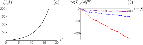
Figure 3: (color online) Numerical demonstrations. The first figure (a) shows $\beta$-dependence of the correlation length $\xi(\beta)$ in the canonical state $\rho_{\beta}$ for one sample of the random Hamiltonian (S.63). The correlation length $\xi(\beta)$ is calculated from the mutual information between the spin pairs of $\{r,n-r+1\}_{r=1}^{n/2}$ with $n=100$. The second figure (b) shows the distance dependence of the mutual information $I_{i,j}(\rho_{\beta})$ for $\beta=3$ (red plots), $\beta=7$ (blue plots), $\beta=13$ (purple plots).

We consider the mutual information $I_{i,j}(\rho_{\beta})$ between the sites $i$ and $j$ is defined as $I_{i,j}(\rho_{\beta})$ for $1\leq\beta\leq 20$. In Fig. 3 (a), we calculate the $\beta$-dependence of the correlation length $\xi(\beta)$. Furthermore, we present the distance dependence of the mutual information $I_{i,j}(\rho_{\beta})$ for $\beta=3$ (red plots), $\beta=7$ (blue plots), $\beta=13$ (purple plots) in Fig. 3 (b). From this plot, the correlation length diverges as $\beta$ increases and the clustering property breaks down at sufficiently low temperatures.

VI Reduced density matrices of $\rho_{{{E}},\Delta}$ and $\rho_{\beta}$ and Theorem 2 in the main text

To compare the result from Theorem 2 with the previous one by Br$\~{a}$ndao and Cramer Brandao and Cramer (2015), we estimate the trace distance between the reduced density matrices of the canonical and micro-canonical states. Let $\{B_{s}\}_{s=1}^{n_{\ell}}$ be the set of all $d$-dimensional $\ell\times\ell\times\cdots\times\ell$ hypercubes (see Fig. 4), where we assume that the total number of hypercubes $n_{\ell}$ is $n/\ell^{d}$ (i.e., $n_{\ell}:=n/\ell^{d}$). We now denote the reduced density matrices within the hypercubes $\{B_{s}\}_{s=1}^{n_{\ell}}$ by $\{(\rho_{\beta})_{B_{s}}\}_{s=1}^{n_{\ell}}$ and $\{(\rho_{{{E}},\Delta})_{B_{s}}\}_{s=1}^{n_{\ell}}$. From theorem 2, we can prove

$$\frac{1}{n_{\ell}}\sum_{s=1}^{n_{\ell}}\left\|(\rho_{{{E}},\Delta})_{B_{s}}-(\rho_{\beta})_{B_{s}}\right\|_{1}\leq \frac{\max\left[c^{\prime}_{1}\ell^{-\frac{d}{2}}\log^{\frac{d+1}{2}}\bigl{(}\frac{\sqrt{n}}{\Delta}\bigr{)},c^{\prime}_{2}\sqrt{\log\bigl{(}\frac{\sqrt{n}}{\Delta}\bigr{)}}\right]}{\sqrt{n_{\ell}}},$$ (S.64)

where $\|\cdots\|_{1}$ denotes the trace norm (see below for the derivation). If we assume the translation invariance of the Hamiltonian (S.1), all the reduced density matrices $\{\rho_{\beta})_{B_{s}},(\rho_{{{E}},\Delta})_{B_{s}}\}_{l=1}^{n_{\ell}}$ do not depend on the index $s$. Hence, for an arbitrary hypercube $B$, the norm difference between $(\rho_{\beta})_{B}$ and $(\rho_{{{E}},\Delta})_{B}$ is smaller than $\mathcal{O}(1/\sqrt{n_{\ell}})$. One of the open problem posed by Brandão and Cramer is how large the block can be in order to guarantee the ensemble equivalence Brandao and Cramer (2015). From the inequality (S.64), provided that $\ell^{d}=\mathcal{O}(n^{1-\epsilon})$ ($\epsilon>0$) and $\Delta=1/{\rm poly}(n)$, the reduced density matrices between the canonical and the microcanonical ensembles are indistinguishable in the limit of $n\to\infty$, where the size dependence of the error behaves as $\mathcal{O}(1/\sqrt{n_{\ell}})=\mathcal{O}(n^{-\epsilon/2})$ with a logarithmic correction ${\rm poly}[\log(n)]$.

The upper bound of (S.64) qualitatively improves the results of previous studies Müller et al. (2015); De Roeck et al. (2006); Lima (1972, 1971); Brandao and Cramer (2015); Tasaki (2018). In Refs Müller et al. (2015); De Roeck et al. (2006); Lima (1972, 1971), the thermodynamic limit $n\to\infty$ has been considered, and the energy width $\Delta$ and block size $\ell$ are assumed to be independent of the system size $n$. In Ref Brandao and Cramer (2015), the finite-size effect has been considered for the first time, where the LHS of (S.64) has been bounded from above by $C\max(\sqrt{\ell^{d(d+1)}/n},n^{-1/(2d+2)})$ with $C={\rm poly}[\log(n)]$ under the assumptions of the clustering and $\Delta=\mathcal{O}(\log^{2d}(n))$. Subsequently, the block size $\ell^{d}$ can be as large as $\ell^{d}=n^{1/(d+1)-\epsilon}$ ($\epsilon>0$). In Ref. Tasaki (2018), this upper bound for the LHS of (S.64) has been improved to $\sqrt{\Delta^{-1}\ell^{d}/n^{1/2}}$ under some additional assumptions. Then, the ensemble equivalence holds for $\ell^{d}=\Delta\cdot n^{1/2-\epsilon}$ ($\epsilon>0$).

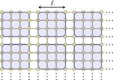
Figure 4: (color online). Schematics of the setup in Ineq. (S.64) on a two-dimensional square lattice. We decompose the lattice to $n_{\ell}$ subsets $\{B_{s}\}_{s=1}^{n_{\ell}}$, each of which contains $\ell\times\ell$ spins ($\ell=4$ in the picture above). We focus on the reduced density matrices with respect to $\{B_{s}\}_{s=1}^{n_{\ell}}$, and estimate the norm difference in Ineq. (S.64) between the canonical and the microcanonical states. From the inequality (S.64), as long as the block size is $\ell^{d}=\mathcal{O}(n^{1-\epsilon})$ ($\epsilon>0$), the ensemble equivalence holds.

VI.1 Proof of the inequality (S.64)

We first consider that for an arbitrary hypercube $B_{s}$, there exists an operator $O_{B_{s}}$ with $\|O_{B_{s}}\|=1$ such that

$$\left\|(\rho_{{{E}},\Delta})_{B_{s}}-(\rho_{\beta})_{B_{s}}\right\|_{1}={\rm tr}\left[O_{B_{s}}\left((\rho_{{{E}},\Delta})_{B_{s}}-(\rho_{\beta})_{B_{s}}\right)\right].$$ (S.65)

We subsequently choose $\Omega=\sum_{i=1}^{n}\Omega_{i}$ as

$$\Omega_{i}=O_{B_{s}}\quad\textrm{for}\quad i\in B_{s},$$ (S.66)

which yields

$$\frac{1}{n}\left|\langle\Omega\rangle_{{{E}},\Delta}-\langle\Omega\rangle_{\beta}\right|= \frac{\ell^{d}}{n}\sum_{s=1}^{n_{\ell}}\left|\langle O_{B_{s}}\rangle_{{{E}},\Delta}-\langle O_{B_{s}}\rangle_{\beta}\right|$$

$$= \frac{1}{n_{\ell}}\sum_{s=1}^{n_{\ell}}\left\|(\rho_{{{E}},\Delta})_{B_{s}}-(\rho_{\beta})_{B_{s}}\right\|_{1},$$ (S.67)

where we use the assumption of $n_{\ell}=n/\ell^{d}$. By combining the inequality (S.67) with Theorem 2 , we obtain the inequality (S.64).

VII Concentration bound from the clustering of correlation

We herein show the proof of Lemma 1 that reduces to the concentration bound (S.17). The proof that we address herein is essentially the same as that of Ref. Anshu (2016) but is more general and simplified. To account for the lattice geometry, we consider a generic graph $G=(V,E)$ with $|V|=n$, where each of the spin sits on the vertex. For two arbitrary subsets $X,Y\subset V$, we define the distance ${\rm dist}(X,Y)$ as the minimum path length from $X$ to $Y$ on the graph. For an arbitrary vertex $i\in V$, we define the set of $X_{i}^{(s)}\in V$ ($s\in\mathbb{N}$) as

$$X_{i}^{(s)}:=\{j\in V|{\rm dist}(j,i)\leq s\}.$$ (S.68)

Each of the local terms $\{\Omega_{i}\}_{i\in V}$ in Eq. (S.7) is supported on the subset $X_{i}^{(\ell)}$. We introduce a geometric parameter $\alpha$ that depends on the lattice structure as

$$|X_{i}^{(s)}|\leq\alpha s^{d},$$ (S.69)

where $d$ is the spatial dimension of the lattice.

VII.1 Proof of Lemma 1

We define $\delta\Omega_{i}:=\Omega_{i}-\langle\Omega_{i}\rangle_{\rho}$ for $\forall i\in V$ that yields $\langle\delta\Omega_{i}\rangle_{\rho}=0$. We calculate the upper bound of $\langle(\Omega-\langle\Omega\rangle_{\rho})^{M}\rangle_{\rho}$, where $M$ is a positive even integer. Next, we decompose

$$\langle(\Omega-\langle\Omega\rangle_{\rho})^{M}\rangle_{\rho}=\sum_{i_{1},i_{2},\ldots i_{M}\in V}\langle\delta\Omega_{i_{1}}\,\delta\Omega_{i_{2}}\,\cdots\,\delta\Omega_{i_{M}}\rangle_{\rho}.$$ (S.70)

We subsequently define $\ell_{i_{1},\ldots,i_{M}}$ as

$$\ell_{i_{1},\ldots,i_{M}}:=\max_{1\leq q\leq M}\left[{\rm dist}(i_{q},\{i_{r}\}_{r\neq q})\right].$$ (S.71)

That is, the most spatially isolated vertex in $\{i_{1},\ldots,i_{M}\}$ is separated from the other vertices by a distance $\ell_{i_{1},\ldots,i_{M}}$. If $\ell_{i_{1},\ldots,i_{M}}=\tilde{l}$, there exists $i_{q}\in\{i_{1},\ldots,i_{M}\}$ such that ${\rm dist}(i_{q},\{i_{r}\}_{r\neq q})=\tilde{l}$. Because each of the $\delta\Omega_{i}$ is supported on the subset $X_{i}^{(\ell)}$ from the assumption (S.7), the two operators $\delta\Omega_{i_{q}}$ and $\delta\Omega_{i_{1}}\cdots\delta\Omega_{i_{q-1}}\delta\Omega_{i_{q+1}}\cdots\delta\Omega_{i_{M}}$ are separated at the least by the distance $\tilde{l}-2\ell$. Hence, for $\tilde{l}\geq 2\ell+r$, the $(r,\xi)$-clustering condition yields

$$|\langle\delta\Omega_{i_{1}}\,\delta\Omega_{i_{2}}\,\cdots\,\delta\Omega_{i_{M}}\rangle_{\rho}-\langle\delta\Omega_{i_{q}}\rangle_{\rho}\langle\delta\Omega_{i_{1}}\,\cdots\,\delta\Omega_{i_{q-1}}\,\delta\Omega_{i_{q+1}}\,\cdots\,\delta\Omega_{i_{M}}\rangle_{\rho}|$$

$$= |\langle\delta\Omega_{i_{1}}\,\delta\Omega_{i_{2}}\,\cdots\,\delta\Omega_{i_{M}}\rangle_{\rho}|\leq 2^{M}e^{-(\tilde{l}-2\ell)/\xi},$$ (S.72)

where we use $\|\delta\Omega_{i}\|\leq 2$ from $\|\Omega_{i}\|\leq 1$ for $\forall i\in V$.

We define $\mathcal{C}_{\tilde{l}}$ ($\mathcal{C}_{\leq\tilde{l}}$) as the set of string $(i_{1},\ldots,i_{M})$ such that $\ell_{i_{1},\ldots,i_{M}}=\tilde{l}$ ($\ell_{i_{1},\ldots,i_{M}}\leq\tilde{l}$). Here, we take the element order in the string into account. For instance, we count $(i_{1},i_{2})$ and $(i_{2},i_{1})$ as a different string if $i_{1}\neq i_{2}$. We subsequently bound $\langle(\Omega-\langle\Omega\rangle_{\rho})^{M}\rangle_{\rho}$ from above as follows:

$$\langle(\Omega-\langle\Omega\rangle_{\rho})^{M}\rangle_{\rho} =\sum_{\tilde{l}=0}^{\infty}\sum_{(i_{1},i_{2},\ldots i_{M})\in\mathcal{C}_{\tilde{l}}}\langle\delta\Omega_{i_{1}}\,\delta\Omega_{i_{2}}\,\cdots\,\delta\Omega_{i_{M}}\rangle_{\rho}$$

$$=\sum_{\tilde{l}=0}^{2\ell+r-1}\sum_{(i_{1},i_{2},\ldots i_{M})\in\mathcal{C}_{\tilde{l}}}\langle\delta\Omega_{i_{1}}\,\delta\Omega_{i_{2}}\,\cdots\,\delta\Omega_{i_{M}}\rangle_{\rho}+\sum_{\tilde{l}=2\ell+r}^{\infty}\sum_{(i_{1},i_{2},\ldots i_{M})\in\mathcal{C}_{\tilde{l}}}\langle\delta\Omega_{i_{1}}\,\delta\Omega_{i_{2}}\,\cdots\,\delta\Omega_{i_{M}}\rangle_{\rho}$$

$$\leq 2^{M}\sum_{\tilde{l}=0}^{2\ell+r-1}\sum_{(i_{1},i_{2},\ldots i_{M})\in\mathcal{C}_{\tilde{l}}}1+2^{M}\sum_{\tilde{l}=2\ell+r}^{\infty}\sum_{(i_{1},i_{2},\ldots i_{M})\in\mathcal{C}_{\tilde{l}}}e^{-(\tilde{l}-2\ell)/\xi}$$

$$\leq 2^{M}\sum_{\tilde{l}=0}^{3\ell}\sum_{(i_{1},i_{2},\ldots i_{M})\in\mathcal{C}_{\tilde{l}}}1+2^{M}\sum_{\tilde{l}=3\ell+1}^{\infty}\sum_{(i_{1},i_{2},\ldots i_{M})\in\mathcal{C}_{\tilde{l}}}e^{-(\tilde{l}-2\ell)/\xi}$$

$$\leq 2^{M}\sum_{(i_{1},i_{2},\ldots i_{M})\in\mathcal{C}_{\leq 3\ell}}1+2^{M}\sum_{\tilde{l}=3\ell+1}^{\infty}\sum_{(i_{1},i_{2},\ldots i_{M})\in\mathcal{C}_{\tilde{l}}}e^{-\tilde{l}/(3\xi)}$$

$$\leq 2^{M}\sum_{(i_{1},i_{2},\ldots i_{M})\in\mathcal{C}_{\leq 3\ell}}1+2^{M}\sum_{\tilde{l}=3\ell+1}^{\infty}\sum_{(i_{1},i_{2},\ldots i_{M})\in\mathcal{C}_{\leq\tilde{l}}}e^{-\tilde{l}/(3\xi)}\,.$$ (S.73)

Herein, we use the inequality (S.72) in the first inequality as well as the relation $\|\delta\Omega_{i}\|\leq 2$. Furthermore, in the second last inequality, we use $e^{-(\tilde{l}-2\ell)/\xi}\leq e^{-\tilde{l}/(3\xi)}$ for $\tilde{l}\geq 3\ell$. At the last inequality, we use a trivial relation where $\mathcal{C}_{\leq\tilde{l}}$ is a larger set than $\mathcal{C}_{\tilde{l}}$.

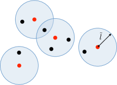
Figure 5: (color online). Schematics of the core vertices (red dots) and the surrounding vertices (black dots). Around each of the core vertices within the distance $\tilde{l}$ (blue shaded region), there exists at least one surrounding vertex. Any string $\{i_{1},\ldots,i_{M}\}\in\mathcal{C}_{\leq\tilde{l}}$ can be decomposed into $u$ core vertices and $(M-u)$ surrounding vertices with $u\leq M/2$.

To count the total number of strings in the set $\mathcal{C}_{\leq\tilde{l}}$, we follow the strategy below. We first choose $u$ “core” vertices $(i_{q_{1}},\ldots,i_{q_{u}})$ from $n$ vertices. We next assign the other $(M-u)$ vertices. We refer to the $(M-u)$ vertices $\{i_{1},\ldots,i_{M}\}\setminus\{i_{q_{1}},\ldots,i_{q_{u}}\}$ as the “surrounding” vertices. Each of the core vertices contains at least one surrounding vertex within the distance $\tilde{l}$ around it (otherwise, the distance $\ell_{i_{1},\ldots,i_{M}}$ exceeds $\tilde{l}$. See the schematics in Fig. 5). Mathematically, for a core vertex $i_{q_{1}}$, there exists $i_{r}\in\{i_{1},\ldots,i_{M}\}\setminus\{i_{q_{1}},\ldots,i_{q_{u}}\}$ such that

$${\rm dist}(i_{q_{1}},i_{r})\leq\tilde{l}\quad{\rm or}\quad i_{r}\in X^{(\tilde{l})}_{i_{q_{1}}}$$ (S.74)

with $X^{(\tilde{l})}_{i_{q_{1}}}$ defined in Eq. (S.68). This constraint implies that the number of core vertices is smaller than $M/2$ (i.e., $u\leq M/2$). We note that any string in $\mathcal{C}_{\leq\tilde{l}}$ can be described by the formalism above. Thus, our task is to count all the possible arrangements of 1) the core vertices, 2) the surrounding vertices for $u=1,2,\ldots,M/2$, and 3) the order of elements in the string. For a fixed $u$, it is bounded from above as follows:

1. The number of possible locations of the core vertices is clearly smaller than $n^{u}$.

2. After the locations of the core vertices are determined, there are at the most $|X^{(\tilde{l})}_{i_{q_{1}}}\cup X^{(\tilde{l})}_{i_{q_{2}}}\cup\cdots\cup X^{(\tilde{l})}_{i_{q_{u}}}|\leq u(\alpha\tilde{l}^{d})$ methods of positioning, at which each of the surrounding vertices can be placed. In total, the number of possible arrangements of the surrounding vertices is smaller than $[u(\alpha\tilde{l}^{d})]^{M-u}$.

3. We next consider the string order. Inside each set of the core and surrounding vertices, the order is already considered by the two estimations above. Hence, we must consider the order of the types of vertices (i.e., “core” and “surrounding”). The number of this combination is $\binom{M}{u}$.

We thus obtain

$$\sum_{(i_{1},i_{2},\ldots i_{M})\in\mathcal{C}_{\leq\tilde{l}}}1\leq\sum_{u=1}^{M/2}\binom{M}{u}n^{u}[u(\alpha\tilde{l}^{d})]^{M-u} \leq[Mn(\alpha\tilde{l}^{d})/2]^{M/2}\sum_{u=1}^{M/2}\binom{M}{u}$$

$$\leq 2^{M}[Mn(\alpha\tilde{l}^{d})/2]^{M/2}=[2Mn(\alpha\tilde{l}^{d})]^{M/2}.$$ (S.75)

By combining the inequality (S.75) with (S.73), we obtain

$$\langle[\Omega]^{M}\rangle_{\rho} \leq[8Mn\alpha(3\ell)^{d}]^{M/2}+\sum_{\tilde{l}=3\ell+1}^{\infty}[8Mn(\alpha\tilde{l}^{d})]^{M/2}e^{-\tilde{l}/(3\xi)}$$

$$\leq[8\alpha Mn(3\ell)^{d}]^{M/2}+3\xi[8\alpha nM^{d+1}(3\xi d/2)^{d}]^{M/2},$$ (S.76)

where the second inequality is given from

$$\sum_{\tilde{l}=3\ell+1}^{\infty}[8Mn(\alpha\tilde{l}^{d})]^{M/2}e^{-\tilde{l}/(3\xi)} \leq(8\alpha Mn)^{M/2}\int_{0}^{\infty}x^{dM/2}e^{-x/(3\xi)}dx$$

$$=(8\alpha Mn)^{M/2}(3\xi)^{dM/2+1}(dM/2)!\leq 3\xi[8\alpha nM^{d+1}(3\xi d/2)^{d}]^{M/2}.$$ (S.77)

Note that we have $s!\leq s^{s}$ for an arbitrary integer $s$. This completes the proof of Lemma 1. $\square$

References

• von Neumann (2010) J. von Neumann, “Proof of the ergodic theorem and the H-theorem in quantum mechanics,” The European Physical Journal H 35, 201–237 (2010).
• Kinoshita et al. (2006) Toshiya Kinoshita, Trevor Wenger,  and David S. Weiss, “A quantum Newton’s cradle,” Nature 440, 900–903 (2006).
• Trotzky et al. (2012) Stefan Trotzky, Yu-Ao Chen, Andreas Flesch, Ian P McCulloch, Ulrich Schollwöck, Jens Eisert,  and Immanuel Bloch, “Probing the relaxation towards equilibrium in an isolated strongly correlated one-dimensional Bose gas,” Nature Physics 8, 325 (2012).
• Gring et al. (2012) M. Gring, M. Kuhnert, T. Langen, T. Kitagawa, B. Rauer, M. Schreitl, I. Mazets, D. Adu Smith, E. Demler,  and J. Schmiedmayer, “Relaxation and Prethermalization in an Isolated Quantum System,” Science 337, 1318–1322 (2012).
• Kaufman et al. (2016) Adam M. Kaufman, M. Eric Tai, Alexander Lukin, Matthew Rispoli, Robert Schittko, Philipp M. Preiss,  and Markus Greiner, “Quantum thermalization through entanglement in an isolated many-body system,” Science 353, 794–800 (2016).
• Tang et al. (2018) Yijun Tang, Wil Kao, Kuan-Yu Li, Sangwon Seo, Krishnanand Mallayya, Marcos Rigol, Sarang Gopalakrishnan,  and Benjamin L. Lev, “Thermalization near Integrability in a Dipolar Quantum Newton’s Cradle,” Phys. Rev. X 8, 021030 (2018).
• Kucsko et al. (2018) G. Kucsko, S. Choi, J. Choi, P. C. Maurer, H. Zhou, R. Landig, H. Sumiya, S. Onoda, J. Isoya, F. Jelezko, E. Demler, N. Y. Yao,  and M. D. Lukin, “Critical Thermalization of a Disordered Dipolar Spin System in Diamond,” Phys. Rev. Lett. 121, 023601 (2018).
• Itoh et al. (2018) Kosuke Itoh, Ryo Nakazawa, Tomoaki Ota, Masayuki Hashisaka, Koji Muraki,  and Toshimasa Fujisawa, “Signatures of a Nonthermal Metastable State in Copropagating Quantum Hall Edge Channels,” Phys. Rev. Lett. 120, 197701 (2018).
• Popescu et al. (2006) Sandu Popescu, Anthony J Short,  and Andreas Winter, “Entanglement and the foundations of statistical mechanics,” Nature Physics 2, 754 (2006).
• Goold et al. (2016) John Goold, Marcus Huber, Arnau Riera, Lídia del Rio,  and Paul Skrzypczyk, “The role of quantum information in thermodynamics—a topical review,” Journal of Physics A: Mathematical and Theoretical 49, 143001 (2016).
• Yukalov (2011) V.I. Yukalov, “Equilibration and thermalization in finite quantum systems,” Laser Physics Letters 8, 485–507 (2011).
• Nandkishore and Huse (2015) Rahul Nandkishore and David A. Huse, “Many-Body Localization and Thermalization in Quantum Statistical Mechanics,” Annual Review of Condensed Matter Physics 6, 15–38 (2015).
• D’Alessio et al. (2016) Luca D’Alessio, Yariv Kafri, Anatoli Polkovnikov,  and Marcos Rigol, “From quantum chaos and eigenstate thermalization to statistical mechanics and thermodynamics,” Advances in Physics 65, 239–362 (2016).
• Gogolin and Eisert (2016) Christian Gogolin and Jens Eisert, “Equilibration, thermalisation, and the emergence of statistical mechanics in closed quantum systems,” Reports on Progress in Physics 79, 056001 (2016).
• Mori et al. (2018) Takashi Mori, Tatsuhiko N Ikeda, Eriko Kaminishi,  and Masahito Ueda, “Thermalization and prethermalization in isolated quantum systems: a theoretical overview,” Journal of Physics B: Atomic, Molecular and Optical Physics 51, 112001 (2018).
• Reimann (2015) Peter Reimann, “Eigenstate thermalization: Deutsch’s approach and beyond,” New Journal of Physics 17, 055025 (2015).
• Deutsch (2018) Joshua M Deutsch, “Eigenstate thermalization hypothesis,” Reports on Progress in Physics 81, 082001 (2018).
• Deutsch (1991) J. M. Deutsch, “Quantum statistical mechanics in a closed system,” Phys. Rev. A 43, 2046–2049 (1991).
• Srednicki (1994) Mark Srednicki, “Chaos and quantum thermalization,” Phys. Rev. E 50, 888–901 (1994).
• Kim et al. (2014) Hyungwon Kim, Tatsuhiko N. Ikeda,  and David A. Huse, “Testing whether all eigenstates obey the eigenstate thermalization hypothesis,” Phys. Rev. E 90, 052105 (2014).
• Mondaini et al. (2016) Rubem Mondaini, Keith R. Fratus, Mark Srednicki,  and Marcos Rigol, “Eigenstate thermalization in the two-dimensional transverse field Ising model,” Phys. Rev. E 93, 032104 (2016).
• Mondaini and Rigol (2017) Rubem Mondaini and Marcos Rigol, “Eigenstate thermalization in the two-dimensional transverse field Ising model. II. Off-diagonal matrix elements of observables,” Phys. Rev. E 96, 012157 (2017).
• Shiraishi and Mori (2017) Naoto Shiraishi and Takashi Mori, “Systematic Construction of Counterexamples to the Eigenstate Thermalization Hypothesis,” Phys. Rev. Lett. 119, 030601 (2017).
• Turner et al. (2018) C. J. Turner, A. A. Michailidis, D. A. Abanin, M. Serbyn,  and Z. Papic, “Weak ergodicity breaking from quantum many-body scars,” Nature Physics 14, 745–749 (2018).
• Lin and Motrunich (2019) Cheng-Ju Lin and Olexei I. Motrunich, “Exact Quantum Many-Body Scar States in the Rydberg-Blockaded Atom Chain,” Phys. Rev. Lett. 122, 173401 (2019).
• Moudgalya et al. (2018) Sanjay Moudgalya, Nicolas Regnault,  and B. Andrei Bernevig, “Entanglement of exact excited states of Affleck-Kennedy-Lieb-Tasaki models: Exact results, many-body scars, and violation of the strong eigenstate thermalization hypothesis,” Phys. Rev. B 98, 235156 (2018).
• Hastings (2007) M. B. Hastings, “Entropy and entanglement in quantum ground states,” Phys. Rev. B 76, 035114 (2007).
• Brandão and Cramer (2015) Fernando G. S. L. Brandão and Marcus Cramer, “Entanglement area law from specific heat capacity,” Phys. Rev. B 92, 115134 (2015).
• Masanes (2009) Lluís Masanes, “Area law for the entropy of low-energy states,” Phys. Rev. A 80, 052104 (2009).
• Brandao and Cramer (2015) Fernando GSL Brandao and Marcus Cramer, “Equivalence of statistical mechanical ensembles for non-critical quantum systems,” arXiv preprint arXiv:1502.03263  (2015), arXiv:1502.03263 .
• Tasaki (2018) Hal Tasaki, “On the Local Equivalence Between the Canonical and the Microcanonical Ensembles for Quantum Spin Systems,” Journal of Statistical Physics 172, 905–926 (2018).
• Alba (2015) Vincenzo Alba, “Eigenstate thermalization hypothesis and integrability in quantum spin chains,” Phys. Rev. B 91, 155123 (2015).
• Araki (1969) Huzihiro Araki, “Gibbs states of a one dimensional quantum lattice,” Communications in Mathematical Physics 14, 120–157 (1969).
• Hernández-Santana et al. (2015) Senaida Hernández-Santana, Arnau Riera, Karen V Hovhannisyan, Martí Perarnau-Llobet, Luca Tagliacozzo,  and Antonio Acín, “Locality of temperature in spin chains,” New Journal of Physics 17, 085007 (2015).
• Park and Yoo (1995) Yong Moon Park and Hyun Jae Yoo, “Uniqueness and clustering properties of Gibbs states for classical and quantum unbounded spin systems,” Journal of Statistical Physics 80, 223–271 (1995).
• Ueltschi (2004) Daniel Ueltschi, “Cluster expansions and correlation functions,” Moscow Mathematical Journal 4, 511–522 (2004).
• Kliesch et al. (2014) M. Kliesch, C. Gogolin, M. J. Kastoryano, A. Riera,  and J. Eisert, “Locality of Temperature,” Phys. Rev. X 4, 031019 (2014).
• Fröhlich and Ueltschi (2015) Jürg Fröhlich and Daniel Ueltschi, “Some properties of correlations of quantum lattice systems in thermal equilibrium,” Journal of Mathematical Physics 56, 053302 (2015).
• Kuwahara et al. (2019) Tomotaka Kuwahara, Kohtaro Kato,  and Fernando Brandão, “Clustering of conditional mutual information for quantum Gibbs states above a threshold temperature,” arXiv preprint arXiv:1910.09425  (2019), arXiv:1910.09425 .
• Thomas and Yin (1983) Lawrence E. Thomas and Zhong Yin, “Low temperature expansions for the Gibbs states of weakly interacting quantum Ising lattice systems,” Communications in Mathematical Physics 91, 405–417 (1983).
• Kennedy (1985) Tom Kennedy, “Long range order in the anisotropic quantum ferromagnetic Heisenberg model,” Communications in Mathematical Physics 100, 447–462 (1985).
• Takahashi (1986) Minoru Takahashi, “Quantum Heisenberg Ferromagnets in One and Two Dimensions at Low Temperature,” Progress of Theoretical Physics Supplement 87, 233–246 (1986).
• Winterfeldt and Ihle (1997) S. Winterfeldt and D. Ihle, “Theory of antiferromagnetic short-range order in the two-dimensional Heisenberg model,” Phys. Rev. B 56, 5535–5541 (1997).
• (44) Supplementary material.
• Biroli et al. (2010) Giulio Biroli, Corinna Kollath,  and Andreas M. Läuchli, “Effect of Rare Fluctuations on the Thermalization of Isolated Quantum Systems,” Phys. Rev. Lett. 105, 250401 (2010).
• Iyoda et al. (2017) Eiki Iyoda, Kazuya Kaneko,  and Takahiro Sagawa, “Fluctuation Theorem for Many-Body Pure Quantum States,” Phys. Rev. Lett. 119, 100601 (2017).
• Kuwahara (2016a) Tomotaka Kuwahara, “Connecting the probability distributions of different operators and generalization of the Chernoff–Hoeffding inequality,” Journal of Statistical Mechanics: Theory and Experiment 2016, 113103 (2016a).
• Anshu (2016) Anurag Anshu, “Concentration bounds for quantum states with finite correlation length on quantum spin lattice systems,” New Journal of Physics 18, 083011 (2016).
• ft (2) If we consider a general value for the energy of the ground state, the same relation can be derived by shifting the eigenenergy $E_{m}$ to $E_{m}-E_{0}$.
• ft (3) More precisely, $\log Z_{\beta^{\ast}}\sim n^{\alpha}$ $(\alpha<1/2)$ is sufficient for convergence in the right-hand side.
• ft (4) For ${\cal N}_{E,1}\leq n^{cE}$ we assume $\beta^{\ast}=c^{\ast}\log n$ satisfying $c^{\ast}>c$. Subsequently, we have $Z_{\beta^{\ast}}=\sum_{m=0}^{2^{n}-1}e^{-\beta^{\ast}E_{m}}\leq 1+\sum_{j\geq 1}(n^{c-c^{\ast}})^{j}$, which is finite even for the thermodynamic limit. Recall that the energy of the ground state is set to zero. Note that in the high-energy regime, the bound (9) is too loose to describe the true system-size dependence of ${\cal N}_{E,1}$, and hence this computation overestimates the amplitude of $Z$ (nevertheless, it is still of $\mathcal{O}(1)$).
• Hastings and Koma (2006) MatthewB. Hastings and Tohru Koma, “Spectral Gap and Exponential Decay of Correlations,” Communications in Mathematical Physics 265, 781–804 (2006).
• Nachtergaele and Sims (2006) Bruno Nachtergaele and Robert Sims, “Lieb-Robinson Bounds and the Exponential Clustering Theorem,” Communications in Mathematical Physics 265, 119–130 (2006).
• Chung and Peschel (2001) Ming-Chiang Chung and Ingo Peschel, “Density-matrix spectra of solvable fermionic systems,” Phys. Rev. B 64, 064412 (2001).
• Lieb et al. (1961) Elliott Lieb, Theodore Schultz,  and Daniel Mattis, “Two soluble models of an antiferromagnetic chain,” Annals of Physics 16, 407 – 466 (1961).
• (56) Note that $2\epsilon_{k}$ for all $k$ are larger than the energy gap. Then, let us define $\tilde{\epsilon}$ as such $2\epsilon_{k}\geq\tilde{\epsilon}$ for all $1\leq k\leq n$. Subsequently, the total number of eigenstates whose energy is smaller than $\bar{q}\tilde{\epsilon}$ is less than $\sum_{q\leq\bar{q}}\binom{n}{q}\leq n^{\bar{q}}$. This implies ${\cal N}_{E,E}\leq n^{E/\tilde{\epsilon}}$, and hence ${\cal N}_{E,1}\leq n^{E/\tilde{\epsilon}}$.
• ft (1) From the inequalities on ${\cal A}_{1}$ and ${\cal A}_{2}$, we can derive conditions $\Delta\geq\sqrt{n}e^{-n^{1/(d+1)}}$ and $\Delta\geq\sqrt{n}e^{-n/\ell^{d}}$, respectively. Since for large $n$ the former inequality is stronger than the latter one, a general lower bound of the energy width is given by (14).
• Lima (1972) R. Lima, “Equivalence of ensembles in quantum lattice systems: States,” Communications in Mathematical Physics 24, 180–192 (1972).
• Lima (1971) R Lima, “Equivalence of ensembles in quantum lattice systems,” Ann. Inst. H. Poincaré Sect. A 15, 61–68 (1971).
• De Roeck et al. (2006) Wojciech De Roeck, Christian Maes,  and Karel Netočnỳ, “Quantum macrostates, equivalence of ensembles, and an H-theorem,” Journal of Mathematical Physics 47, 073303 (2006).
• Müller et al. (2015) Markus P. Müller, Emily Adlam, Lluís Masanes,  and Nathan Wiebe, “Thermalization and Canonical Typicality in Translation-Invariant Quantum Lattice Systems,” Communications in Mathematical Physics 340, 499–561 (2015).
• Georgii (1995) Hans-Otto Georgii, “The equivalence of ensembles for classical systems of particles,” Journal of Statistical Physics 80, 1341–1378 (1995).
• Touchette (2011) H. Touchette, “Ensemble equivalence for general many-body systems,” EPL (Europhysics Letters) 96, 50010 (2011).
• Touchette (2015) Hugo Touchette, “Equivalence and Nonequivalence of Ensembles: Thermodynamic, Macrostate, and Measure Levels,” Journal of Statistical Physics 159, 987–1016 (2015).
• Rigol et al. (2007) Marcos Rigol, Vanja Dunjko, Vladimir Yurovsky,  and Maxim Olshanii, “Relaxation in a Completely Integrable Many-Body Quantum System: An Ab Initio Study of the Dynamics of the Highly Excited States of 1D Lattice Hard-Core Bosons,” Phys. Rev. Lett. 98, 050405 (2007).
• Calabrese et al. (2011) Pasquale Calabrese, Fabian H. L. Essler,  and Maurizio Fagotti, “Quantum Quench in the Transverse-Field Ising Chain,” Phys. Rev. Lett. 106, 227203 (2011).
• Kuwahara (2016b) Tomotaka Kuwahara, “Asymptotic behavior of macroscopic observables in generic spin systems,” Journal of Statistical Mechanics: Theory and Experiment 2016, 053103 (2016b).
• Kuwahara et al. (2017) Tomotaka Kuwahara, Itai Arad, Luigi Amico,  and Vlatko Vedral, “Local reversibility and entanglement structure of many-body ground states,” Quantum Science and Technology 2, 015005 (2017).
• Kuwahara and Saito (2019) Tomotaka Kuwahara and Keiji Saito, “Gaussian concentration bound and Ensemble equivalence in generic quantum many-body systems including long-range interaction,” arXiv preprint arXiv:1906.10872  (2019), arXiv:1906.10872 .
Supplementary Material for
“Ensemble equivalence and eigenstate thermalization from clustering of correlation”
Tomotaka Kuwahara1,2 and Keiji Saito3
1Mathematical Science Team, RIKEN Center for Advanced Intelligence Project (AIP),1-4-1 Nihonbashi, Chuo-ku, Tokyo 103-0027, Japan
2Interdisciplinary Theoretical & Mathematical Sciences Program (iTHEMS) RIKEN 2-1, Hirosawa, Wako, Saitama 351-0198, Japan
3Department of Physics, Keio University, Yokohama 223-8522, Japan