Multi-frequency scatter broadening evolution of pulsars - II. Scatter broadening of nearby pulsars

Abstract

We present multi-frequency scatter broadening evolution of 29 pulsars observed with the LOw Frequency ARray (LOFAR) and Long Wavelength Array (LWA). We conducted new observations using LOFAR Low Band Antennae (LBA) as well as utilized the archival data from LOFAR and LWA. This study has increased the total of all multi-frequency or wide-band scattering measurements up to a dispersion measure (DM) of 150 pc cm^-3 by 60%. The scatter broadening timescale ($\tau_{sc}$) measurements at different frequencies are often combined by scaling them to a common reference frequency of 1 GHz. Using our data, we show that the $\tau_{sc}$–DM variations are best fitted for reference frequencies close to 200–300 MHz, and scaling to higher or lower frequencies results in significantly more scatter in data. We suggest that this effect might indicate a frequency dependence of the scatter broadening scaling index ($\alpha$). However, a selection bias due to our chosen observing frequencies can not be ruled out with the current data set. Our data did not favour any particular model of the DM – $\tau_{sc}$ relations, and we do not see a statistically significant break at the low DM range in this relation. The turbulence spectral index ($\beta$) is found to be steeper than that is expected from a Kolmogorov spectrum. This indicates that the local ISM turbulence may have a low wave-number cutoff or presence of large scale inhomogeneities in the line of sight to some of the reported pulsars.

1 Introduction

Pulsed radio signals from pulsars get scattered due to multi-path propagation while traveling through the irregularities in the ionized inter-stellar medium (IISM), resulting in broadening of the pulse profile. This scatter broadening is a highly frequency dependent phenomenon, with the characteristic pulse broadening time, $\tau_{sc}$, scaling with the observing frequency, $\nu$, in the form of $\tau_{sc}\propto\nu^{-\alpha}$ (Rickett, 1977), where $\alpha$ is the frequency scaling index. Consequently, the nearby pulsars (low DM) show prominent scatter-broadening primarily at low radio frequencies ($<$ 1.0 GHz), while the distant pulsars (high DM) show measurable scattering effects up to much higher radio frequencies (a few GHz) and disappear completely as a pulsed source at low frequencies. The evolution of scatter-broadening of pulsar signal over frequencies provides insights into the turbulence characteristics of the IISM and allows a study of the clumps and hollows in the IISM in detail.

The multi-path propagation of the signal creates a diffraction pattern at the observer’s plane that decorrelates over a characteristic bandwidth $\delta\nu_{d}$, such that 2$\pi\tau_{sc}\delta\nu_{d}=C_{1}$. The constant $C_{1}$ is expected to be of the order of unity for a Kolmogorov type turbulence (Cordes, Weisberg & Boriakoff, 1985). Following Rickett (1977) and Armstrong, Rickett & Spangler (1995), the power spectrum of electron density irregularities for an isotropic homogeneous medium can be shown as

$$P_{n_{e}}(q)=C_{n_{e}}^{{}^{2}}(q^{2}+l_{o}^{-2})^{-\beta/2}exp(-q^{2}l_{i}^{2}/2),$$ (1)

where $P_{n_{e}}(q)$ is the power spectrum density of irregularities, $C_{n_{e}}^{{}^{2}}$ is the scattering strength of the medium, $q$ is the three dimensional wavenumber, $\beta$ is the spectral index, $l_{o}$ and $l_{i}$ are the outer and inner scales of turbulence. This can be simplified further, if $l_{i}<1/q<l_{o}$ to $P_{n_{e}}(q)=C^{2}_{n_{e}}q^{-\beta}$. By combining different measurements of ISM effects, like dispersion, scattering, Faraday rotation, etc. on pulsars with distances $\leq$1 kpc, Armstrong, Rickett & Spangler (1995) found that the electron density turbulence is close to Kolmogorov model with an upper limit on the inner scale of turbulence as 10⁸m. As mentioned above, $\tau_{sc}$ increases with decreasing observing frequency, and its frequency scaling index is related to $\beta$ via $\alpha=2\beta/(\beta-2)$ (for $2<\beta<4$). For a Gaussian distribution of irregularities, it was found that $\tau_{sc}\propto\nu^{-4}$ DM² (Rickett, 1977). For the Kolmogorov turbulence model, one expects $\beta=11/3$, and consequently the scaling relation changes to $\tau_{sc}\propto\nu^{-4.4}$ DM^2.2 (Romani, Narayan & Blandford, 1986). Goodman & Narayan (1985) worked out the relations for the cases where $\beta$ was found to be more than the critical value of 4. They speculated, with the then available data, that $\beta$ is 4.3 in general, instead of the 11/3 expected for a medium with Kolmogorov turbulence.

Several studies have been conducted in the past to understand the turbulence in the IISM by using different techniques. Cordes, Weisberg & Boriakoff (1985) studied the scintillation characteristics of a large sample of pulsars, and found that the IISM turbulence follows Kolmogorov turbulence very well in nearby regions ($\leq$ 2kpc). Löhmer et al. (2001, 2004) studied moderate to high DM pulsars with multi-frequency scatter-broadening measurements and proposed that the IISM tends to follow Kolmogorov turbulence up to about a DM of 350 pc cm^-3 and deviates from it beyond this. Lewandowski et al. (2015b) analyzed a large sample of scatter-broadening measurements (60 pulsars) to understand the characteristics of the IISM. They suggested that the IISM as a whole follows Kolmogorov turbulence characteristics. Krishnakumar et al. (2017, hereafter referred as KJM17) undertook an extensive study of multi-frequency scatter-broadening of 39 pulsars using the Ooty Radio Telescope (ORT) and the Giant Metrewave Radio Telescope (GMRT), which increased the total number of available $\alpha$ measurements by about 50%. They found that several nearby pulsars show a flatter $\alpha$ than expected. A study by Geyer et al. (2017) on scatter-broadening evolution of 13 low DM pulsars using the LOw Frequency ARray (LOFAR) also showed that most of the nearby pulsars have a shallower $\alpha$ ($<4$). They also noted that there may be a frequency dependent evolution of $\alpha$, after comparing their measurements with those at higher frequencies. One of the possibilities is that the pulsars in the supernova remnants or those with lines-of-sight passing through HII regions show a flatter $\alpha$ (Goodman & Narayan, 1985), however, this has not been explored in detail so far.

In all the earlier studies, very few measurements of scatter-broadening of low DM pulsars were included. This made it difficult to understand the turbulence characteristics in the local IISM. It has not been clear, with the sparse amount of data available so far, whether the turbulence characteristics are Kolmogorov or not at low DMs. As explained above, it is expected that $\tau_{sc}$ $\propto$ DM^2.2 at low DMs and becomes steeper at high DMs. With the introduction of new low frequency telescopes with wide-band receivers and improved back-ends, we are now able to observe the in-band evolution of scatter-broadening of many low DM pulsars. In this study, we have made new observations as well as analyzed archival data of a large sample of low DM pulsars over multiple frequencies or by using data from large fractional bandwidth receivers to better understand the $\tau_{sc}-$DM dependence. With the advantage of having wide-band observations, we also measure and study in-band evolution of the frequency scaling index of scattering ($\alpha$) for these pulsars.

In this study, we aim to (1) estimate $\alpha$ for a large set of pulsars below a DM of $\sim$150 pc cm^-3, (2) confirm or rule-out previously reported dip in $\alpha-$DM relation around a DM of $\sim$100 pc cm^-3 with better statistics, (3) model the DM$-\tau_{sc}$ relationship, and (4) examine for HII region or Nebula associations in the directions of the pulsars. The observations and analyses are described in Section 2 followed by our main results (Section 3). Section 4 presents a discussion of our results, and we summarize and conclude in Section 5.

2 Observations and Data Analysis

2.1 Observations and data reduction

The data used in this paper were obtained from new observations with LOFAR as well as from the archived ones from both LOFAR and Long Wavelength Array (LWA). The LOFAR telescope has a seamless frequency coverage from $\sim$30 MHz to $\sim$240 MHz (van Haarlem et al., 2013). We have used the Low Band Array (LBA; 30$-$80 MHz) to observe 31 pulsars. The observations were performed between December 2016 and May 2017 in several different sessions. The voltage beam data were coherently dedispersed by the observatory using the PulP pipeline on CEP3 cluster (Kondratiev et al., 2016) available at the facility. The dedispersed data were further processed using the PSRCHIVE package (Hotan et al., 2004) to excise radio frequency interference, correct for any possible slight inaccuracies in pulsar period and DM from the ephemerides and then reduced to sub-banded profiles for further processing. Although we observed 31 pulsars below a DM of 100 pc cm^-3, processing of the data for pulsars with DMs above 40 pc cm^-3 was not possible due to some technical issues with the then available version of the PulP. Additionally, there were other factors during our observations which reduced the overall achievable sensitivity. We could detect 15 pulsars from our full list. Moreover, the signal-to-noise ratio (S/N) was not adequate enough for many of these to measure scatter broadening of the average profile or of those in separate parts of the band (for fitting purpose, we have used only profiles having a peak S/N ratio of at least 6 in this paper). We were able to measure $\tau_{sc}$ for 8 pulsars and estimate $\alpha$ for 6 of these using the sub-band data. There were not enough sub-band profiles with S/N ratio larger than 6 for the remaining two pulsars.

We used the LOFAR archival data reported in Bilous et al. (2016); Pilia et al. (2016) utilizing the High Band Array (HBA) in the frequency range of 110$-$190 MHz. We re-processed the data using PSRCHIVE package to correct for any small inaccuracies in period and DM, and reduced these to sub-banded profiles. Depending on the sensitivity of detection, we used different number of sub-bands for each pulsar (typically 10 or 20) across the band. We measured $\tau_{sc}$ evolution across the band for a total of 14 pulsars combining data from other high frequency observations from the EPN data archive and from the ORT and GMRT (see KJM17 for the profiles and $\tau_{sc}$ estimates).

The LWA is a multipurpose radio telescope operating in the frequency range of 10 – 88 MHz (See Ellingson et al., 2009, for more information about LWA). With the first station of LWA, namely LWA1, located near the Very Large Array (VLA) in New Mexico, Stovall et al. (2015) reported the detection of 44 pulsars. These data are publicly available through the LWA data archive. We chose a set of 10 pulsars from this archive, which show clear evolution of scatter-broadening and have peak S/N ratio larger than 6 even when the full band is divided in to 8 or 16 sub-bands for measuring $\tau_{sc}$. The data were reduced using PSRCHIVE package and analyzed further to measure $\tau_{sc}$.

Some of the pulsar profiles are scatter-broadened over the entire band of LOFAR and LWA. Finding a good template for the fitting procedure, detailed in the next session, was difficult from the archival data-sets for such pulsars. We observed a sub-set of pulsars from this list, which were within the declination coverage limits ($-60>\delta<+60$) of the ORT. ORT is operating at a central frequency of 326.5 MHz with a bandwidth of 16 MHz. It is an ideal instrument to provide template profiles since frequency of observations of such templates will be close to the LWA and LOFAR frequencies and yet show no scatter-broadening. Hence, the effects due to profile evolution will be limited, in contrast with measurements using a higher frequency template. The observations were made using the PONDER back-end (Naidu et al., 2015) with the ORT during MJDs 57963 – 57964. We detected 15 pulsars with good S/N ratio $(>20)$ and used their profiles as templates for fitting. Out of the 15 detected pulsars, six were used as templates for HBA data, three each for LWA and LBA data and three for the data taken from LBA, HBA as well as LWA. For pulsars that were not detected (or were beyond the declination limits) at ORT, we used the nearest high frequency profiles from the EPN database. Most of these profiles were obtained from the Lovell telescope (Gould & Lyne, 1998) except one, which was from Arecibo (Sayer, Nice & Taylor, 1997), as mentioned in Table 1.

2.2 Analysis

The average profiles, and in many cases the sub-band profiles, obtained from the above analysis were further used for obtaining $\tau_{sc}$ by the method detailed in KJM17. Briefly, the scattered pulse profile can be represented as a convolution of the intrinsic pulse, $P_{i}(t)$, with the impulse response characterizing the scatter-broadening in the IISM, $s(t)$, the dispersion smear across the narrow spectral channel, D(t), and the instrumental impulse response, $i(t)$. The instrumental impulse response is small enough to neglect, since the rise times of the receivers and back-ends are very small. Hence, we have the scattered pulse as

$$P(t)=P_{i}(t)\ast s(t)\ast D(t)$$ (2)

We followed the same method as detailed in KJM17 to extract $\tau_{sc}$, where we used a high frequency, unscattered profile for convolving with the impulse response of IISM, which can be expressed as

$$s(t)=\exp(-t/\tau_{sc})U(t)$$ (3)

where U(t) is a unit step function.

The data from LOFAR were coherently dedispersed, so the effect of $D(t)$ in Equation 2 can be neglected. LWA data on the other hand were incoherently dedispersed, with a specific channel resolution. This introduces an increase in the observed pulse profile width. We convolved the template profiles with the estimated dispersion smearing before fitting for scatter-broadening in such cases, to minimize any contamination of the resultant measurements.

After measuring $\tau_{sc}$ for each of the sub-banded profiles, we used a Monte-Carlo method described in KJM17 for estimating the frequency scaling index, $\alpha$. For $\tau_{sc}$ estimates at each of the sub-bands, we generated 10,000 normally distributed random numbers with the root-mean-square deviation same as the error bars on $\tau_{sc}$. To estimate $\alpha$, a power-law fit was made to these randomly generated $\tau_{sc}$ values at different frequencies. We report the median of these $\alpha$ values, with error bars from 5 and 95 percentiles, in Table 1. Some of the pulse profiles at the lower frequency end look very noisy, mostly because of the large number of bins which is kept same for all the sub-bands. The uncertainties are naturally large for the $\tau_{sc}$ measurements of such sub-band profiles. The $\alpha$ measurements take in to account the uncertainties on $\tau$, and hence, are not affected by such low S/N profiles. In any case, we confirmed that the final value of $\alpha$ did not show any deviations beyond the limits yielded from the Monte-Carlo method, when we tried removing those noisy lower-frequency profiles from the analysis.

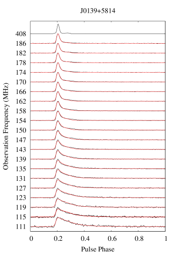
Figure 1: Frequency evolution of scatter broadening for PSR J0139+5814. Left panel shows the pulse profiles at different frequencies as labeled in the abscissa. The profile at the top is the template profile used for fitting purpose to estimate $\tau_{sc}$. The black color curves are observed profiles at different frequencies and the red curves are the best fit models. Right panel shows $\tau_{sc}$ as a function of observing frequency. The black filled circles are the measured $\tau_{sc}$ and the black continuous line is the fit to the complete data. The dashed line represents the trend corresponding to the typical Kolmogorov spectrum value of 4.4. Errorbars on $\tau_{sc}$ are smaller than the symbol sizes.

3 Results

We report scatter-broadening measurements of 31 pulsars, and $\alpha$ estimates for 29 of these. The results are summarized in Table 1, with details like, pulsar name in J2000 coordinates, period, DM, distance, number of bins in the profiles, range of frequencies from which $\tau_{sc}$ is estimated, reference template frequency, and value of $\alpha$ and $\tau_{sc}$ scaled to 200 MHz. The last column lists the telescopes used in this study, in the ascending order of frequencies, with the highest frequency providing the template obtained from the telescope mentioned last. A sample plot of the scatter broadening evolution of PSR J0139+5814 is shown in Figure 1. The left hand side panel shows the sub-band integrated pulse profiles at different frequencies obtained using the HBA of LOFAR, where one can see a clear evolution of scatter broadening as a function of frequency. We have used a high frequency profile as a template for estimating the scatter broadening, which, in this case, is the profile at 408 MHz from the Lovell telescope, as shown at the top of the panel. The right hand side panel shows fit for estimating $\alpha$. No measurement of $\alpha$ was possible for pulsars where $\tau_{sc}$ could be estimated for only two or less frequencies. For these pulsars, estimates of $\tau_{sc}$, scaled to 200 MHz by using $\alpha=4$ are also listed in Table 1. Out of the 31 pulsars, 14 are from the HBA archival data, 7 are from the LWA archival data, 7 are from our observations with the LBA, an additional one is common between both the LWA archive and the LBA observations, and another two are common between both the LWA and the HBA archives. This study has increased the total set of $\alpha$ measurements below a DM of $\sim$100 pc cm^-3 by two folds. The $\alpha$ value estimated in this study ranges between 2.4$-$5.7. We note that several pulsars in this DM range show a flatter $\alpha$ than what was reported previously by Cordes, Weisberg & Boriakoff (1985) and Johnston et al. (1998), using decorrelation bandwidth measurements. This can also be seen in the recent results from Geyer et al. (2017) and KJM17.

Five of our pulsars are common to Geyer et al. (2017), viz., PSRs J0040+5716, J0117+5914, J0543+2329, J1851+1259 and J1913$-$0440. Geyer et al. (2017) measured scatter broadening by simultaneously fitting for both $\tau_{sc}$ and the intrinsic profile width, $P_{i}(t)$. Since the intrinsic pulse width is unknown and is also found to increase with decreasing observing frequency in general(Thorsett, 1991; Pilia et al., 2016), a fit to both these parameters make it difficult to decouple scattering effects from profile evolution. In addition, the pulse broadening functions used in Geyer et al. (2017) are different, hence our results cannot be directly compared with those reported by them. While profile evolution can also affect our analysis, making the lowest frequency $\tau_{sc}$ measurement an over estimate, we used unscattered profile at a nearby frequency (mostly with ORT at 327 MHz) to mitigate this effect. For a fair comparison, we reanalyzed the data for these five pulsars using Geyer et al. (2017) methods. We find that the measurements of $\alpha$ are consistent with their results within error bars for PSRs J0040+5716, J0117+5914, J0543+2329 and J1851+1259 with both their anisotropic and isotropic models. In case of PSR J1913$-$0440, our $\alpha$ is steeper than that from both of their models by about three times the standard deviation. However, this is perhaps due to the fact that we did not have access to data below 148 MHz for this pulsar. Thus, our estimates of $\alpha$ from independent measurements of $\tau_{sc}$ are consistent with the previously reported values.

There are six pulsars in our data-set where the profiles have multiple components. Two of them (PSRs J0406+6138 and J0629+2415) show the steepest $\alpha$ in our list, while the rest four (PSRs J0139+5814, J0525+1115, J2149+6329 and 2229+6205) exhibit flatter $\alpha$. It is not clear whether profile evolution has affected these measurements, but we do not see any significant profile evolution between the template profile and the highest frequency profile in the HBA band, where $\tau_{sc}$ is measured. Although there is large amount of scatter broadening for three of them, the two pulsars with steep $\alpha$ have $\tau_{sc}$ less than 10% of the period at the lowest frequency in HBA. Hence, to clearly understand whether our measurements are affected by profile evolution, we require lower frequency observations (LWA/LBA frequencies), where the scatter-broadening will dominate the intrinsic pulse width evolution. In case of the four flatter $\alpha$ pulsars, except for PSR J0139+5814, the other three are heavily scatter-broadened. Hence, it is unlikely that the intrinsic profile width evolution had any significant effect on the measured $\alpha$.

Two pulsars (PSRs J1645–0317 and J1752–2806) in our sample have previous $\alpha$ measurements available in the literature (Cordes, Weisberg & Boriakoff, 1985) and two others (PSRs J0358+5413 and J0826+2637) have multi-frequency decorrelation bandwidth ($\delta\nu_{d}$) estimates. Cordes, Weisberg & Boriakoff (1985) report $\alpha$ of $4.5\pm 0.4$ and $4.7\pm 0.3$ for PSR J1645–0317 and PSR J1752–2806, respectively, using $\delta\nu_{d}$ and $\tau_{sc}$ estimates made at discrete frequencies between 80 and 1400 MHz. They had only one low frequency $\tau_{sc}$ estimate (at 80 MHz) while all other measurements were $\delta\nu_{d}$ estimates from higher frequency observations. With the data presented here, our estimates of $\alpha$ are 4.1$\pm$0.6 and 3.7$\pm$0.2 respectively for these pulsars. It can be seen that $\alpha$ is different for PSR J1752–2806 while it is consistent within limits for PSR J1645–0317. The change in $\alpha$ for PSR J1752–2806 might indicate the possibility of its frequency dependence, if it is not caused by an erroneous value of $C_{1}$ or due to changes in the IISM turbulence characteristics over several years. For the other two pulsars, we found $\delta\nu_{d}$ measurements at higher frequencies ($>$ 400 MHz) from Cordes, Weisberg & Boriakoff (1985). The $\alpha$ values obtained after combining with our data set are different than what is reported here ($\alpha=3.5\pm 0.1$ for PSR J0358+5413 and $\alpha=4.8\pm 0.1$ for PSR J0826+2637). Without a good understanding of the actual value of $C_{1}$, combining the $\delta\nu_{d}$ data with $\tau_{sc}$ measurements might give incorrect results. Since we do not have the measured value of $C_{1}$, we used the theoretical value of unity, for demonstrating various possibilities that may affect the determination of $\alpha$. The changes in the combined data of the latter pulsars may be due to either a frequency dependence of $\alpha$ or as in the previous case, due to the slow long-term variations in the IISM turbulence. We are unable to make any claim of a frequency dependence of $\alpha$ on the basis of this data combination, due to the unavailability of simultaneous multi-frequency data across a wide range of frequencies and the lack of knowledge of the actual value of $C_{1}$, while converting from $\delta\nu_{d}$ to $\tau_{sc}$.

With this study, the total number of $\alpha$ measurements have increased to 111. Further, below a DM of 200 pc cm^-3, this number has increased to 83, around 50% increase from the sample that was available with KJM17. A dip at around a DM of 100 pc cm^-3 was reported by KJM17 as well as by Geyer et al. (2017). As discussed in the following section, we do not see this dip in our now statistically large sample.

4 Discussions

4.1 DM dependence of scattering

Rickett (1977) suggested that there is probably a power-law relation between DM and $\delta\nu_{d}$, although the number of available measurements were very less at that time. If the scattering material is distributed uniformly along the distance to the pulsar, then $\tau_{sc}\propto$ DM² and for a power-law turbulence with Kolmogorov spectrum characteristics, $\tau_{sc}\propto$ DM^2.2. Later, Slee et al. (1980) extended the sample with scintillation and scatter-broadening measurements of 31 pulsars and reported a power-law relation between DM and $\tau_{sc}$ with a power-law index of 3.5$\pm$0.2. Alurkar, Slee & Bobra (1986) found a similar relation ($\tau_{sc}\propto$DM^3.3±0.2) using a sample of 85 pulsars. These results indicated that the $\tau_{sc}$ – DM relationship is much steeper than what was expected from a Kolmogorov spectrum of turbulence and requires a higher $\beta$. Goodman & Narayan (1985) realized this problem and suggested that this can be accommodated by theory within the range of $4<\beta<6$. They also argued that this may be due to scattering from large scale inhomogeneities in the line of sight to the pulsar.

Bhattacharya et al. (1992) fitted a broken power-law (sum of two power-laws) to the $\tau_{sc}-$DM relation, since they saw a flattening from a simple power-law spectrum at low DMs (below a DM of $\sim$30 pc cm^-3). Their fit showed that the measured $\tau_{sc}$ follows Kolmogorov turbulence at low DMs and deviates at higher DMs. This was adapted in many later works (Ramachandran et al., 1997). Similarly, Bhat et al. (2004) used a simple parabolic curve for fitting 371 $\tau_{sc}$ measurements at different frequencies and estimated $\alpha$ to be 3.86$\pm$0.16, i.e., much less than 4.4 expected for a medium with Kolmogorov turbulence. In these studies, $\tau_{sc}$ was scaled to a reference frequency (typically 1 GHz) assuming a constant $\alpha$. In contrast, Lewandowski et al. (2015b) scaled the $\tau_{sc}$ by using the $\alpha$ obtained from the measurements till then (60 pulsars) to 1 GHz, before studying its dependence with DM. With the new $\alpha$ estimates from KJM17, Geyer et al. (2017), and those from this study, which has increased the sample by about 2 folds (111 pulsars) from what was available with Lewandowski et al. (2015b), we try to re-examine these relations.

Available measurements of $\alpha$ typically have 5$-$10$\%$ uncertainties. Thus, scaling $\tau_{sc}$ from the frequency of its estimate to a widely different frequency is likely to not only yield an over-estimate of uncertainty at the reference frequency, but also an increased scatter. Thus, high frequency measurements of $\tau_{sc}$ will yield large scatter at low reference frequency and vice-verse. While Krishnakumar et al. (2015) estimated $\tau_{sc}$ for a large number of pulsars at a single frequency of 326.5 MHz, this is not possible for the pulsar population as a whole as $\tau_{sc}-$DM relation implies significant scattering for low DM pulsars at frequencies only below 300 MHz and reliable measurements for high DM pulsars possible only for frequencies above 1 GHz. Thus, an optimum reference frequency needs to be chosen for comparison of variations in $\tau_{sc}$ as a function of DM.

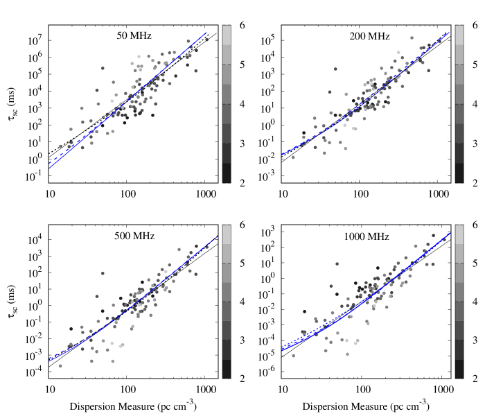
Figure 2: The panels of the figure show the scaled $\tau_{sc}$ against DM plotted at 50, 200 500 MHz and 1 GHz. The blue continuous and dashed curves represent the fit of broken power laws, as given in Equation 4. Black dashed curve is the fit of a parabolic function following the relation in Equation 5 and black continuous line is the fit by a simple power-law. The $\tau_{sc}$ measurements are plotted with a color scheme of light gray to dark gray as a function of their $\alpha$ value in steps of 0.5 between $2<\alpha<6$. The data used in this plot are taken from Löhmer et al. (2001, 2004), Lewandowski et al. (2013, 2015a, 2015b), Geyer et al. (2017), KJM17 and this study.

Before scaling $\tau_{sc}$ to a standard frequency of 1 GHz, it is worthwhile to check if 1 GHz is the optimum frequency for scaling all these measurements, since almost all of the $\tau_{sc}$ measurements were obtained below 1 GHz. We first chose a set of trial reference frequencies between 30 and 1000 MHz, each separated by 50 MHz. A plot of scaled $\tau_{sc}$ at 50 MHz, 200 MHz 500 MHz and 1 GHz are given in Figure 2 for comparison. Then, for each of the trial reference frequencies, we scaled $\tau_{sc}$ using the best fit parameters obtained while fitting for $\alpha$. We fitted a simple power-law as was done by Slee et al. (1980); Alurkar, Slee & Bobra (1986) and computed reduced $\chi^{2}$ of the fit. Although the $\chi^{2}$ of the fits are very high, it does vary significantly with chosen reference frequency for scaling, as shown in Figure 3. It is clear that the minimum of the $\chi^{2}$ for our data set is around 200 MHz, indicating that the scatter in the plot is minimized at this frequency. Thus, we chose 200 MHz as a reference frequency for comparison of different models. The model relations we chose from the literature are (1) a simple power law model (Slee et al., 1980; Alurkar, Slee & Bobra, 1986), (2) a broken power law model as in Equation 4, (3) a broken power law model by fixing the value of $\zeta=2.2$ in Equation 4 (Bhattacharya et al., 1992; Ramachandran et al., 1997), and (4) a second order polynomial fit following Bhat et al. (2004) as given in Equation 5. Since we measured $\alpha$ for the pulsars used in this study, we have scaled $\tau_{sc}$ using it and removed the last term in Equation 5 while fitting (Lewandowski et al., 2015a; Geyer et al., 2017).

Figure 3: The plot shows the reduced $\chi^{2}$ of a simple power-law fit to the whole data set of $\tau_{sc}$ against DM as a function of reference frequency. The black points denote the reduced $\chi^{2}$ at each frequency where a fit was performed.

$$\tau_{sc}=aDM^{\zeta}({1+bDM^{\gamma}})$$ (4)

$$log\tau_{sc}=a+b(logDM)+c(logDM)^{2}-\alpha log\nu$$ (5)

The power law fit to the 200 MHz data yielded $\tau_{sc}=DM^{3.4}/10^{5.6}$, with a reduced $\chi^{2}$ of 44. The broken power law model, following Equation 4 gave $\tau_{sc}=1.09\times 10^{-4}DM^{2.2}({1+2.7\times 10^{-3}DM^{1.65}})$ with a reduced $\chi^{2}$ of 31. The broken power law model with the value of $\zeta$ fixed at 2.2 gave $\tau_{sc}=9.95\times 10^{-5}DM^{2.2}({1+1.5\times 10^{-3}DM^{1.7}})$ with a reduced $\chi^{2}$ of 29. The second order polynomial, following Equation 5 (after removing the last term of $\alpha$) yielded $log\tau_{sc}=-4.01+1.68(logDM)+0.45(logDM)^{2}$ with a reduced $\chi^{2}$ of 37. Above fits do not really favour any particular relations. The difference between various fitted forms will be more apparent at very low or high DMs. The current data set is insufficient to examine this due to the unavailability of a large number of $\alpha$ of pulsars below a DM of 30 pc cm^-3 and no $\alpha$ measurements below a DM of 10 pc cm^-3 from scatter broadening measurements. Thus, populating this DM range with new $\alpha$ estimates from telescopes with wide-band receivers, such as LWA, LOFAR and future Square Kilometer Array, will be helpful in clarifying this issue.

Our fit to Equation 5 shows that there is a strong linear dependence in the DM – $\tau_{sc}$ relation than what was reported by Bhat et al. (2004). Lewandowski et al. (2015b) and Geyer et al. (2017) also reported a strong dependence on the linear term than the quadratic one. We also find that the scatter in our plots vary as a function of DM (as also demonstrated above using Figure 2). At very low frequencies, i.e., below $\sim$100 MHz, although the $\tau_{sc}$ of low DM pulsars seem cluster together, the high DM ones are scattered across a large range. Likewise, at high frequencies, the scatter is high for low DM pulsars but is less for high DM pulsars. This change of scatter may be due to the frequency dependence of $\alpha$ or due to the fact that the $\tau_{sc}$ measurements of these pulsars were done at around these frequencies. Although there can be other reasons for scatter in measurements of $\tau_{sc}$, such as a low wave number cut-off in the turbulence spectrum or a non-Kolmogorov type turbulence in the line of sight, our analysis does indicate that there is a possibility for a frequency dependence of $\alpha$. Further wide-band multi-frequency observations are required to confirm or disprove this effect.

4.2 Turbulence characteristics of the IISM

A plot of $\alpha$ against DM and distance to the pulsar are given in the top and bottom panels of Figure 4. The plot is now mainly populated by measurements from this study and KJM17 up to a DM of $\sim$300 pc cm^-3. The $\alpha$ measurements are scattered across a large range, but mostly below the conventional value of 4 or 4.4, at all DM and distance ranges. Unlike what was reported in KJM17, we do not see any clear dip in $\alpha$ at around a DM of 100 pc cm^-3. A closer inspection of the data from KJM17 and this study show that most of the pulsars with low $\alpha$ values around 100 pc cm^-3 are concentrated behind the Sagittarius arm and some are behind HII regions or supernova remnants. A list of pulsars behind the HII regions and supernova remnants is given in Table 2. The table lists, against each pulsar, the DM, distance estimated from the DM, distance estimated from parallax measurements, HII region along the line of sight to the pulsar and the distance to it and the $\alpha$ estimates. It should be noted that only some of the pulsars listed in the table show a flatter $\alpha$ than the average value. Few low DM pulsars, without any associations, also show a low value of $\alpha$, as can be realized from Table 1 , which may be due to a low wave-number cut-off in the turbulence spectrum at our low observing frequencies, affecting the measured $\alpha$ values as put forward by Goodman & Narayan (1985), or due to anisotropic scattering screens (Geyer et al., 2017). A detailed investigation of these effects is beyond the scope of the present work.

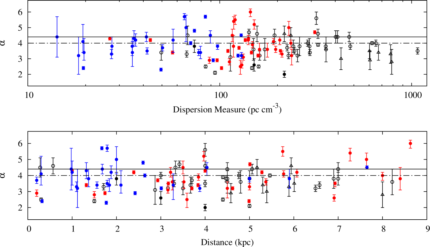
Figure 4: The figure shows the distribution of $\alpha$ as a function of DM and distance. Black open circles denote measurements from Lewandowski et al. (2013, 2015a, 2015b); black filled circles are measurements from Geyer et al. (2017); black open triangles are from Löhmer et al. (2001, 2004); red filled circles denote measurements from KJM17 and blue filled circles are from this study. The black solid line indicate $\alpha$ = 4.4 and black dash-dotted line shows $\alpha$ = 4.

The turbulence spectral index, $\beta$, can be estimated from $\alpha$, for a power-law wave-number spectrum using the relations put forward by Goodman & Narayan (1985), Cordes, Pidwerbetsky & Lovelace (1986) and Romani, Narayan & Blandford (1986) as given below

$$\alpha=\begin{cases}\frac{2\beta}{\beta-2}&\quad 2<\beta<4\\ \frac{8}{6-\beta}&\quad 4<\beta<6.\end{cases}$$ (6)

The two regions of $\beta$ differ essentially due to the difference in the scale sizes of the scattering regions involved; for $\beta<4$, the scattering comes from the small scales($10^{9}-10^{12}$ cm), while for $\beta>4$, the scales involved are much larger ($10^{12}-10^{15}$ cm). In addition, for the $\beta>4$ region, the effect of refractive scattering is large and is independent of observing frequency and distance to the pulsar (Goodman & Narayan, 1985).

The distribution of the $\alpha$ values is not normal, and has a skewness of 0.3. Hence, estimating the average value of $\alpha$ might give wrong estimate. Hence, we report the median of this distribution with limits from the lower and higher quartiles as 3.7${}^{+0.6}_{-0.7}$. A similar distribution for both the relations in equation 6, is also calculated, only with larger skewness (mostly due to the effect of large/small values of $\beta$ near the boundaries) which makes median statistics a better estimate. The median value of this distribution of $\beta$ values came to be 4.2${}^{+0.9}_{-0.6}$ and 3.8$\pm$0.3 respectively, for both the models. Goodman & Narayan (1985) assumed $\beta$ to be 4.3 for their discussions and were supported by observations from other fields also (see Goodman & Narayan (1985) for more details). As is evident from our data-set, $\beta$ is much higher than $11/3$ and indicates that the turbulence spectra is steeper than the Kolmogorov model with a small inner scale. Following Armstrong, Rickett & Spangler (1995) we estimated the power spectral density of scattering for all of the reported pulsars reported here and almost all the points followed the slope of the power spectrum with an inner scale ($l_{i}$) of 10⁵ m and an outer scale ($l_{o}$) of 10¹⁸ m, indicating that the effects of innerscale of turbulence is hard to decipher with the current data set and will require future observations.

5 Summary and Conclusions

We have reported multi-frequency scatter-broadening measurements of 31 pulsars, along with frequency scaling index ($\alpha$) for 29 of these. This sample increases the number of the $\alpha$ measurements so far by about 30% and almost doubles the sample below a DM of $\sim$100 pc cm^-3. With this enriched data-set, we analyze the DM dependence of scattering. We find that the scatter in the $\tau_{sc}$ – DM dependence changes as a function of reference frequency and hence scaling all the measurements to a standard frequency of 1 GHz, as was done in earlier studies, is not a good practice. This analysis also indicates that there is a possibility for $\alpha$ to be frequency-dependent, in addition to other effects which may cause this scatter. We tried to fit a power-law after scaling all the 111 measurements till date to different reference frequencies and find that around 200 – 300 MHz is the best range for fitting the DM – $\tau_{sc}$ relations, since the scatter in the data is minimal at those reference frequencies. Furthermore, we find no significant difference between fits to different $\tau_{sc}$ – DM relations in the literature, although a broken power-law fit seems to give the smallest reduced $\chi^{2}$. We find that $\alpha$ for many of the pulsars at low DMs in the current sample is consistently lower than the standard value of 4.4 for a Kolmogorov spectrum. This indicate that there may be a wave-number cut-off in these lines of sight or the presence of inhomogeneities like HII regions, stellar winds, supernova remnants, etc. The median value of $\alpha$ was found to be 3.7${}^{+0.6}_{-0.7}$. We have also estimated the turbulence spectral index, $\beta$ for all the pulsars and found that the median value is 4.2${}^{+0.9}_{-0.6}$ and 3.8$\pm$0.3 for the expressions of $\alpha$ given in Equation 6. These values are higher than what is expected for a Kolmogorov spectrum ($\beta$=11/3) and is consistent with results from scattering in other fields (Goodman & Narayan, 1985). We did not find any significant evidence for a flattening of $\alpha$ around a DM of $\sim$100 pc cm^-3 which indicates that this inference was perhaps biased by the sample selection. We also find that line of sight to some of the pulsars in the sample pass through HII regions or supernova remnants. Many of these pulsars show a flatter $\alpha$ than 4.4, indicating that the large electron number density, and hence turbulence of these regions, might affect scatter-broadening.

Further investigations are required to study the frequency dependence of $\alpha$, where low frequency telescopes with wide-band receivers such as LOFAR, LWA and SKA would play a vital role. Multi-frequency observations of a carefully chosen set pulsars will help further exploring any frequency dependence of $\alpha$ and we are in the process of conducting such observations in near future.

Acknowledgment: We thank the anonymous referee for detailed suggestions which helped in improving the manuscript substantially. We are grateful to Annya Bilous and Maura Pilia for sharing partially reduced archival LOFAR data with us. YM acknowledges use of the funding from the European Research Council under the European Union’s Seventh Framework Programme (FP/2007-2013)/ERC Grant Agreement no. 617199. This paper is based (in part) on data obtained with the International LOFAR Telescope (ILT) under project code LC7_029. LOFAR (van Haarlem et al., 2013) is the Low Frequency Array designed and constructed by ASTRON. It has observing, data processing, and data storage facilities in several countries, that are owned by various parties (each with their own funding sources), and that are collectively operated by the ILT foundation under a joint scientific policy. We thank the scientists at LOFAR, particularly Sander ter Veen, for the support with our observations and processing on CEP3. We thank the LWA consortium for making their data publicly available. Support for operations and development of the LWA1 is provided by the National Science Foundation of the University Radio Observatory program. Basic research on pulsars at NRL is supported by the Chief of Naval Research (CNR). We also thank the technicians at the ORT for their support during the observations. We acknowledge support from Department of Science and Technology grant DST-SERB Extra-mural grant EMR/2015/000515.

Table 1: Measurements of $\alpha$ for pulsars from our analysis. Each column gives pulsar name in J2000, Period in seconds, DM in pc cm^-3, Distance derived from YMW16 model (Yao, Manchester & Wang, 2017), Number of phase bins used in the profile, Frequency range of $\tau_{sc}$ measurements, Template profile frequency used for fitting, $\alpha$ estimated, $\tau_{sc}$ scaled to 200 MHz and the telescope(s) used. An asterisk with the distance estimate show that it is a DM independent distance estimate. For pulsars which do not have $\alpha$ estimates, the $\tau_{sc}$ is scaled assuming $\alpha=4$ and are marked by a $\dagger$.

PSR J	Period	DM	Dist.	Bins	Freq. range	Templ. Freq.	$\alpha$	$\tau_{sc}$	Telescopes
	(s)	pc cm-3	(kpc)		(MHz)	(MHz)		(ms)
J0040+5716	1.118225	92.51	2.42	512	111.8 – 186.1	408	2.9${}^{+0.1}_{-0.1}$	17 $\pm$ 1	HBA; LOVELL
J0117+5914	0.101439	49.42	1.77	256	111.8 – 186.1	610	2.2${}^{+0.1}_{-0.1}$	3.5 $\pm$ 0.2	HBA; LOVELL
J0139+5814	0.272451	73.81	2.60*	256	111.8 – 143.1	408	3.1${}^{+0.1}_{-0.1}$	1.9 $\pm$ 0.1	HBA; LOVELL
J0358+5413	0.156384	57.14	1.00*	256	47.35 – 81.62	327	4.6${}^{+0.7}_{-0.8}$	0.1 $\pm$ 0.1	LWA; LOVELL
J0406+6138	0.594576	65.41	1.79	256	111.8 – 158.7	408	5.7${}^{+0.2}_{-0.2}$	1.0 $\pm$ 0.1	HBA; LOVELL
J0415+6954	0.390715	27.45	1.37	512	115.7 – 143.1	327	3.8${}^{+0.6}_{-0.5}$	0.7 $\pm$ 0.2	HBA; ORT
J0502+4654	0.638565	41.83	1.32	128	145.0 – 408.0	610	3.5${}^{+0.2}_{-0.2}$	100 $\pm$ 50	HBA; GMRT; ORT; LOVELL
J0525+1115	0.354438	79.42	1.84	256	113.8 – 152.8	327	3.4${}^{+0.4}_{-0.4}$	4.4 $\pm$ 0.8	HBA; ORT
J0543+2329	0.245975	77.70	1.56	256	113.8 – 176.3	327	3.4${}^{+0.2}_{-0.2}$	2.0 $\pm$ 0.3	HBA; ORT
J0629+2415	0.476623	84.18	1.67	512	111.8 – 154.9	327	5.7${}^{+0.1}_{-0.1}$	0.54 $\pm$ 0.03	HBA; ORT
J0826+2637	0.530661	19.48	0.32*	512	32.65 – 62.05	327	2.4${}^{+0.1}_{-0.1}$	0.06 $\pm$ 0.01	LWA; ORT
J0922+0638	0.430627	27.30	1.10*	512	32.81 – 47.46	327	3.3${}^{+0.3}_{-0.3}$	0.05 $\pm$ 0.02	LBA; ORT
J1509+5531	0.739682	19.62	2.10*	512	37.61 – 71.87	150	3.4${}^{+0.9}_{-0.5}$	0.1 $\pm$ 0.1	LBA; HBA
J1543$-$0620	0.709064	18.38	1.12	256	42.58 – 57.22	150	3.2${}^{+1.2}_{-1.2}$	0.1 $\pm$ 0.1	LBA; HBA
J1543+0929	0.748448	34.98	5.90*	256	52.25 – 85.93	150	3.8${}^{+0.6}_{-0.6}$	0.7 $\pm$ 0.4	LWA; HBA
J1645$-$0317	0.387690	35.76	1.32	256	42.92 – 66.95	327	4.1${}^{+0.5}_{-0.6}$	0.011 $\pm$ 0.004	LWA; LBA; ORT
J1752$-$2806	0.562558	50.37	0.20*	256	66.94 – 146.48	327	3.7${}^{+0.2}_{-0.2}$	1.5 $\pm$ 1.0	LWA; HBA; ORT
J1758+3030	0.947256	35.07	3.28	256	47.35 – 76.75	370	2.2${}^{+1.0}_{-1.0}$	1.2 $\pm$ 0.5	LWA; ARECIBO
J1823+0550	0.752907	66.78	2.00*	512	47.35 – 71.85	327	4.5${}^{+1.1}_{-1.4}$	0.1 $\pm$ 0.1	LWA; ORT
J1825$-$0935	0.769006	19.38	0.30*	256	42.58 – 76.76	327	4.0${}^{+1.0}_{-0.7}$	0.1 $\pm$ 0.1	LBA; ORT
J1841+0912$\dagger$	0.381319	49.16	1.66	128	63	142	–	0.3 $\pm$ 0.1	LBA; HBA
J1844+1454	0.375463	41.49	1.68	256	42.13 – 86.01	327	4.4${}^{+0.3}_{-0.3}$	0.09 $\pm$ 0.04	LWA; ORT
J1851+1259	1.205303	70.63	2.64	1024	111.8 – 154.8	327	4.0${}^{+0.2}_{-0.2}$	1.1 $\pm$ 0.2	HBA; ORT
J1913$-$0440	0.825936	89.39	4.04	256	66.95 – 147.75	327	4.5${}^{+0.3}_{-0.5}$	4 $\pm$ 3	LWA; HBA; ORT
J1948+3540	0.717311	129.37	7.65	1024	178.2 – 610.0	925	4.5${}^{+0.1}_{-0.1}$	339 $\pm$ 24	HBA; ORT; LOVELL
J2018+2839	0.557953	14.20	0.98*	512	37.21 – 57.22	327	4.4${}^{+1.3}_{-1.3}$	0.02 $\pm$ 0.01	LBA; ORT
J2055+3630	0.221508	97.42	5.00*	256	145.0 – 408.0	610	3.8${}^{+0.1}_{-0.2}$	45 $\pm$ 5	HBA; GMRT; ORT; LOVELL
J2149+6329	0.380140	129.72	3.88	512	111.8 – 170.4	186	3.0${}^{+0.2}_{-0.2}$	11 $\pm$ 1	HBA
J2225+6535	0.682542	36.44	1.88	256	42.41 – 85.82	150	4.2${}^{+0.6}_{-0.7}$	0.1 $\pm$ 0.1	LWA; HBA
J2229+6205	0.443055	124.64	3.01	512	115.7 – 170.5	610	3.2${}^{+0.1}_{-0.1}$	15 $\pm$ 1	HBA; LOVELL
J2337+6151$\dagger$	0.495370	58.41	0.70	512	65	142	–	0.2 $\pm$ 0.1	LBA; HBA

Table 2: This table lists the pulsars for which the line of sight pass through an HII region or is associated with the supernova remnant. Table lists the pulsar name, DM, DM distance (D_DM), DM independent distance(D_A), Association, Distance (D_HII) and $\alpha$. The pulsars in the table include $\alpha$ values from the literature as given in the caption of Figure 2. The details about the pulsar distances are obtained from Manchester et al. (2005) and the associations are obtained from H$\alpha$ maps (Finkbeiner, 2003).

PSR J	DM	DDM	DA	Association	Distance	$\alpha$
	pc cm-3	(kpc)	(kpc)		(kpc)
J0358+5413	57.14	1.00	1.00${}^{+0.20}_{-0.10}$	Sh2–205	1.00$\pm$0.20	4.6${}^{+0.7}_{-0.8}$
J0502+4654	41.83	1.32	–	Sh2–221	0.80$\pm$0.40	3.5${}^{+0.2}_{-0.2}$
J0525+1115	79.42	1.84	–	Sh2–264	0.34	3.4${}^{+0.4}_{-0.4}$
J0534+2200	56.77	2.00	2.00${}^{+0.50}_{-0.50}$	Crab nebula	2.00$\pm$0.50	3.4${}^{+0.2}_{-0.2}$
J0614+2229	96.91	1.74	–	Sh2-248	1.50	2.9${}^{+0.1}_{-0.1}$
J0742-2822	73.78	2.00	2.00${}^{+1.00}_{-0.80}$	Gum nebula	0.40	3.8${}^{+0.4}_{-0.4}$
J0835-4510	67.99	0.28	0.28${}^{+0.02}_{-0.02}$	Gum nebula	0.40	4.5${}^{+0.6}_{-0.6}$
J0837-4135	147.29	1.50	1.50${}^{+1.20}_{-0.90}$	Gum nebula	0.40	2.4${}^{+0.1}_{-0.1}$
J0840-5332	156.50	0.57	–	Gum nebula	0.40	4.6${}^{+0.5}_{-0.5}$
J2029+3744	190.66	5.77	–	Sh–109	1.40	4.1${}^{+0.2}_{-0.2}$
J2055+3630	97.42	5.00	5.00${}^{+0.80}_{-0.60}$	Sh–109	1.40	3.8${}^{+0.1}_{-0.2}$

References

- Alurkar, Slee & Bobra (1986) Alurkar, S. K., Slee, O. B. & Bobra, A. D., 1986, AuJPh, 39, 433
- Armstrong, Rickett & Spangler (1995) Armstrong, J. W., Rickett, B. J. & Spangler, S. R., 1995, ApJ, 443, 209
- Bhat et al. (2004) Bhat, N. D. R., Cordes, J. M., Camilo, F., Nice, D. J. & Lorimer, D. R., 2004, ApJ, 605, 759