Efficient quantum gates for individual nuclear spin qubits by indirect control

Abstract

Hybrid quantum registers, such as electron-nuclear spin systems, have emerged as promising hardware for implementing quantum information and computing protocols in scalable systems. Nevertheless, the coherent control of such systems still faces challenges. Particularly, the lower gyromagnetic ratios of the nuclear spins cause them to respond slowly to control fields, resulting in gate times that are generally longer than the coherence time of the electron. Here, we demonstrate a scheme for circumventing this problem by indirect control: We apply a small number of short pulses only to the electron and let the full system undergo free evolution under the hyperfine coupling between the pulses. Using this scheme, we realize robust quantum gates in an electron-nuclear spin system, including a Hadamard gate on the nuclear spin and a controlled-NOT gate with the nuclear spin as the target qubit. The durations of these gates are shorter than the electron coherence time, and thus additional operations to extend the system coherence time are not needed. Our demonstration serves as a proof of concept for achieving efficient coherent control of electron-nuclear spin systems, such as NV centers in diamond. Our scheme is still applicable when the nuclear spins are only weakly coupled to the electron.

Spin-based quantum registers have come up as a feasible architecture for implementing quantum computing Nielsen and Chuang (2002); Stolze and Suter (2008). Among them are the hybrid systems consisting of electron and nuclear spins such as Nitrogen Vacancy (NV) centers in diamond Gaebel et al. (2006); Neumann et al. (2008); Wrachtrup et al. (2001); Suter and Jelezko (2017); Childress et al. (2006); Fuchs et al. (2009); Balasubramanian et al. (2009); Maurer et al. (2012); Herbschleb et al. (2019); Bradley et al. (2019); Gali et al. (2008). Specific properties of their subsystems are the distinct gyromagnetic ratios, which result, e.g. in the requirement that the frequencies of the control fields applied to electronic and nuclear spins lie in the microwave (MW) and radiofrequency (RF) regimes respectively. The fast gate operation times on the electrons (order of ns) and the long coherence times of the nuclear spins (order of ms) serve as efficient control and memory channels. However, the lower gyromagnetic ratios of the nuclear spins result in longer nuclear spin gate operation times (a few tens of $\mu$s), which can exceed the electron coherence times ($\approx 1-25$ $\mu$s) at room temperature, thus posing a major challenge for coherent control of electron-nuclear spin systems. Techniques like dynamical decoupling (DD) can partly alleviate this issue by extending the coherence times of the electron Meiboom and Gill (1958); Uhrig (2007); Zhang and Suter (2015); Van der Sar et al. (2012); Suter and Álvarez (2016); Zhang et al. (2014), but the additional DD pulses increase the control cost.

Previously, one- and two-qubit operations were demonstrated using RF pulses on the nuclear spin that had strong hyperfine coupling of $\approx 130$ MHz Jelezko et al. (2004); Shim et al. (2013); Rao and Suter (2016). Such strong couplings enhance the nuclear spin Rabi frequency allowing fast RF operations (order of ns) and hence direct control of nuclear spins was feasible Maze et al. (2008); Shim et al. (2013). However, scalable quantum computing requires coherent control of tens to hundreds of qubits and the control of dipolar coupled nuclear spins gets challenging with increasing distance from the electrons. To avoid these challenges, indirect control (IC) of the nuclear spins has also been incorporated Khaneja (2007); Wang et al. (2017); Zhang et al. (2011); Hodges et al. (2008); Cappellaro et al. (2009); Taminiau et al. (2012); Aiello and Cappellaro (2015). In this approach, the control fields are applied only on the electron, combined with free evolution of the system under the hyperfine couplings. However, most of the earlier works based on IC required a large number of control operations, thereby increasing the control overhead Taminiau et al. (2014); Hodges et al. (2008).

In this letter, we experimentally implement efficient quantum gates in an NV center in diamond at room temperature, using IC with minimal control cost of only 2-3 of short MW pulses and delays. Our approach allows variable delays and pulse parameters. As such, it differs from earlier work Taminiau et al. (2014) that used many DD cycles with fixed delays. We use this approach to demonstrate quantum gates that are required for a universal set of gates: a Hadamard gate on a nuclear spin, and a controlled-NOT (CNOT) gate with control on the electron and target on the nuclear spin.

We consider a single NV center that consists of a spin-1 electron coupled to a spin-1 ¹⁴N and a spin-$1/2$ ¹³C [see supplementary material not (a)]. We perform the operations on the electron and ¹³C by focussing on a subspace of the system where the ¹⁴N is in the $m_{N}=1$ state. We then can write the secular part of the electron-¹³C Hamiltonian in the lab frame as ${\cal{H}}/(2\pi)=D(S_{z}^{2}\otimes E_{2})-(\nu_{e}-A_{N})(S_{z}\otimes E_{2})-\nu_{C}(E_{3}\otimes I_{z})+A_{zz}(S_{z}\otimes I_{z})+A_{zx}(S_{z}\otimes I_{x}),$ where $S_{z}$ and $I_{z/x}$ are the spin operators for electron and ¹³C respectively, $E_{n}$ is an $n\times n$ identity matrix, $D=2.87$ GHz is the zero field splitting, $\nu_{e}=-414$ MHz and $\nu_{C}=0.158$ MHz are the Larmor frequencies of the electron and ¹³C in a $14.8$ mT field, $A_{N}=-2.16$ MHz is the hyperfine coupling with ¹⁴N and $A_{zz}=-0.152$ MHz and $A_{zx}=0.110$ MHz are the hyperfine couplings with ¹³C. The eigenstates of ${\cal{H}}$ are $|0\uparrow\rangle,|0\downarrow\rangle,|-1\varphi_{-}\rangle,|-1\psi_{-}\rangle,|1\varphi_{+}\rangle,|1\psi_{+}\rangle$, where $\{|0\rangle,|\pm 1\rangle\}$ are the eigenstates of $S_{z}$, and

$$|\varphi_{\pm}\rangle = \cos(\kappa_{\pm}/2)|\uparrow\rangle+\sin(\kappa_{\pm}/2)|\downarrow\rangle$$

$$|\psi_{\pm}\rangle = -\sin(\kappa_{\pm}/2)|\uparrow\rangle+\cos(\kappa_{\pm}/2)|\downarrow\rangle.$$ (1)

Here $\{|\uparrow\rangle$,$|\downarrow\rangle\}$ are the eigenstates of $I_{z}$, and $\kappa_{\pm}=\arctan[A_{zx}/(A_{zz}\mp\nu_{C})]$ is the angle between the quantization axis of the ¹³C and the NV axis.

We implement the quantum gates $U_{T}$ in the $m_{S}=\{0,-1\}$ and $m_{N}=1$ manifold and refer to it as the system subspace.This choice of subspace is realized by using MW pulses with a Rabi frequency of $\approx 0.5$ MHz ($\ll A_{N})$, which covers all ESR transitions in the system subspace but leaves states untouched where the ¹⁴N is in a different state. For the system subspace, the Hamiltonian is ${\cal H}_{s}/(2\pi)=|0\rangle\langle 0|\otimes{\cal H}_{0}+|-1\rangle\langle-1|\otimes{\cal H}_{-1}$, where ${\cal H}_{0}=-\nu_{C}I_{z}$ and ${\cal H}_{-1}=-(\nu_{C}+A_{zz})I_{z}-A_{zx}I_{x}$ are ¹³C spin Hamiltonians when the electron is in $|0\rangle$ or $|-1\rangle$ respectively.

We implement two examples of $U_{T}$:

$$U_{H} = E_{2}\otimes\begin{bmatrix}1&1\\ 1&-1\end{bmatrix}/\sqrt{2}$$

$$U_{CNOT} = |0\rangle\langle 0|\otimes E_{2}+|-1\rangle\langle-1|\otimes e^{-i\pi I_{x}}.$$ (2)

The first is a Hadamard gate while the second is a CNOT gate, both targeting ¹³C, in a basis defined in Ref. not (b). To check the implementation of $U_{T}$, we initialize the system into a pure state, apply $U_{T}$ and then perform a partial tomography of the final state by recording free precession signals (FIDs).

	$\tau_{1}$	$\tau_{2}$	$\tau_{3}$	$\tau_{4}$	$t_{1}$	$t_{2}$	$t_{3}$	$\phi_{1}$	$\phi_{2}$	$\phi_{3}$
$U_{H}$	$0.74$	$0.22$	$0.43$	$0.89$	$0.23$	$1.26$	$1.50$	$3\pi/2$	$3\pi/2$	$\pi/2$
$U_{CNOT}$	$3.78$	$2.11$	$2.15$	$0.63$	$1.88$	$3.96$	$1.90$	$0$	$\pi/5$	$\pi/2$

Table 1: MW pulse sequence parameters for $U_{H}$ and $U_{CNOT}$. The time durations and phases are in units of $\mu$s and radians respectively.

For practical applications, it is useful to allow additional degrees of freedom, such as variable pulse rotation angles and finite pulse durations. These degrees of freedom allow us to compensate experimental errors via numerical optimization of the pulse sequence parameters. As shown in Fig. 7, we consider a pulse sequence consisting of delays $\tau_{i}$ and MW pulses with durations $t_{i}$ and phases $\phi_{i}$ where $i=1\cdots n$, $n$ is the number of pulses. We fix the frequency of the pulses to be resonant with the ESR transition $0\leftrightarrow-1$ and the Rabi frequency $\omega_{1}/2\pi$ to $0.5$ MHz. During $\tau_{i}$, the system freely evolves under ${\cal{H}}_{s}$ such that $U_{i}^{f}=e^{-i{\cal{H}}_{s}\tau_{i}}$. The control Hamiltonians during the MW pulse segments are ${\cal{H}}_{i}^{MW}=\omega_{1}[\cos\phi_{i}(s_{x}\otimes E_{2})+\sin\phi_{i}(s_{y}\otimes E_{2})]+{\cal{H}}_{s}$, where $s_{x/y}$ denote the spin-1/2 operators for the electron, and the corresponding operators are $U_{i}^{MW}=e^{-i{\cal{H}}_{i}^{MW}t_{i}}$. The total propagator $U$ is the time ordered product of $U_{i}^{f}$ and $U_{i}^{MW}$. The overlap between $U$ and $U_{T}$ is defined by the fidelity $F=|\mathrm{Tr}(U^{\dagger}U_{T})|/4$. We maximize $F$ numerically, using a MATLAB^® subroutine implementing a genetic algorithm Mitchell (1998). The solution returns the pulse sequence parameters $t_{i}$, $\tau_{i}$ and $\phi_{i}$. The sequences were made robust against fluctuations of the MW pulse amplitude by optimizing $F$ over a range $\omega_{1}/(2\pi)=[0.48,0.52]$ MHz. Table 1 summarizes the optimized pulse parameters for $U_{H}$ and $U_{CNOT}$, and the average gate fidelities are $>96\%$ and $>97\%$ respectively. The resulting trajectories of the electron and ¹³C on the Bloch-sphere is shown in the SM not (a).

Our experiments started with an initial laser pulse with a wavelength of $532$ nm, a duration of $5$ $\mu$s, and a power of $\approx 0.5$ mW which initialized the electron to $|0\rangle$ but left the ¹³C in a mixed state. To initialize ¹³C to $|\uparrow\rangle$, we resorted to the IC method Zhang et al. (2019, 2018a); not (a). Starting from $\psi_{0}=|0\uparrow\rangle$, we implemented the circuits shown in Figs. (2, 3). Depending on the experiment, we either observed the electron or the ¹³C state via FID measurements. The readout process consisted of another laser pulse with the same wavelength and $400$ ns duration and was used to measure the population of $m_{S}=0$.

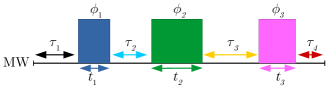
Figure 1: MW pulse sequence to realize $U_{T}$ by IC, at a fixed $\omega_{1}$. The delays $\tau_{i}$, MW pulse durations $t_{i}$ and phases $\phi_{i}$ are the free variables to be optimized.

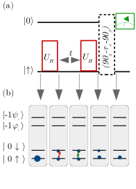
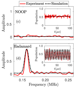
Figure 2: (a) Quantum circuit to test $U_{H}$. The MW pulse sequence parameters for $U_{H}$ are given in Table. 1. The clean-up operation is represented by the dotted box. (b) Populations (solid circles) and coherences (zig-zag arrows) at each stage of the pulse sequence in (a). (c, d) ¹³C spin spectra obtained by the pulse sequence in (a). (c) Without the first $U_{H}$. (d) With both $U_{H}$. Inset: Final population of $|0\uparrow\rangle$ as a function of $t$.

Fig. 2(a) shows the pulse sequence for implementing and detecting the effect of $U_{H}$. The first $U_{H}$ generates $|0\rangle\otimes(|\uparrow\rangle+|\downarrow\rangle)/\sqrt{2}$. The ¹³C coherence is then allowed to evolve for a variable time $t$ after which we apply another $U_{H}$ to convert one component of the coherence to population. Lastly, a clean-up operation, with MW pulse sequence $(90_{x}-\tau_{c}-90_{y})$, where $90_{x/y}$ are pulses with rotation angle $90^{\circ}$ about the $x/y$-axis applied to the $m_{S}=0\leftrightarrow 1$ transition with 0.5 MHz Rabi frequency and $\tau_{c}=1/(2|A_{zz}|)$ is the delay, represented by the dotted box transfers the population from $|0\downarrow\rangle$ to $|1\downarrow\rangle$. The final read-out operation thus detects only the population of $|0\uparrow\rangle$, which depends on $t$ as $[1+\cos(2\pi\nu_{C}t)]/2$. In the frequency domain, this corresponds to a peak at $\nu_{C}$.

Using the pulse sequence in Fig. 2(a), we performed two experiments to compare the effect of $U_{H}$: (1) without the first $U_{H}$ (i.e, no operation, also known as NOOP) and (2) with both $U_{H}$. In the case of NOOP, the system was in $\psi_{0}$ during the free evolution period. Since $\psi_{0}$ does not contain ¹³C coherence the resulting frequency domain signal does not contain a resonance at $\nu_{C}$, as shown in Fig. 2(c). With both $U_{H}$ present, we observe in Fig. 2(d) a resonance peak at $\nu_{C}$ as expected. We numerically simulated the pulse sequence in Fig. 2(a) without and with the first $U_{H}$, and then calculated the final populations of $|0\uparrow\rangle$ as a function of $t$. To match the theoretical signal with the experimental one, we had to scale it by a factor $0.9$ for NOOP and $0.8$ for $U_{H}$ (i.e, with two $U_{H}$), and estimated the infidelity of the experimental $U_{H}$ as $\approx 10\%$.

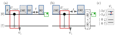
Figure 3: Quantum circuits to test $U_{CNOT}$. The MW pulse sequence parameters for $U_{CNOT}$ indicated by red empty boxes are given in Table. 1. $\theta_{x/y/\phi}$ denote operations with rotation angles $\theta$ about the $x/y/\phi$ axes that are resonant with the transition $0\leftrightarrow-1$ and with Rabi frequencies of $8$ MHz. (a) Pulse sequence to demonstrate the effect of $U_{CNOT}$ on different input states via electron spin detection. $\phi$ is the detuning phase. In the presence (absence) of the $180_{y}$ operation indicated by the dashed box, the FID measurement is used to determine the population of the $m_{S}=-1$ ($m_{S}=0$) after $U_{CNOT}$. (b) Pulse sequence to demonstrate the effect of $U_{CNOT}$ via ¹³C spin detection. (c) Pictorial representation of state $\psi_{1}$.

The schemes to demonstrate $U_{CNOT}$ are shown in Fig. 3. Using the pulse sequence in Fig. 3(a), we demonstrated the effect of $U_{CNOT}$ in $m_{S}=-1$ by measuring electron spin spectra. Choosing for the flip-angle $\theta$ of the initial $\theta_{y}$ operation not (c); Cavanagh et al. (1995) a value of $\pi$, we exchanged the populations of the $|0\uparrow\rangle$ $\leftrightarrow|-1\uparrow\rangle\approx|-1\rangle\otimes(|\phi_{-}\rangle-|\psi_{-}\rangle)/\sqrt{2}$ according to Eq. (1). The subsequent $U_{CNOT}$ transformed $|-1\uparrow\rangle$ to $-i|-1\downarrow\rangle\approx-i|-1\rangle\otimes(|\phi_{-}\rangle+|\psi_{-}\rangle)/\sqrt{2}$, since by definition of Eq. (2), $U_{CNOT}$ flips the ¹³C state when the electron is in $|-1\rangle$. To measure the state after $U_{CNOT}$, we transferred the population of $|-1\downarrow\rangle$ to $|0\downarrow\rangle$ using a hard $180_{y}$ operation. The readout process, which measures the population of $m_{S}=0$, can then be used to determine the population left in $|-1\downarrow\rangle$ by $U_{CNOT}$. The sequence $(90_{x}-t-90_{\phi})$ in Fig. 3(a) implements the electron spin FID measurement, where the $90_{x}$ pulse creates electron coherence and the $90_{\phi}$ pulse converts one component of the evolved coherence to population Suter and Jelezko (2017); Zhang et al. (2018a). Here we incremented the phase $\phi(t)=-2\pi\nu_{d}t$ linearly with $t$, using a detuning frequency $\nu_{d}$ of 3 MHz. We then measured the population of $m_{S}=0$ with the readout laser pulse as a function of $t$ and its Fourier transform gives the frequency domain signal. Thus, as seen in the electron spin spectra in Fig. 4(a), the change of nuclear spin state resulted in a different frequency of the ESR lines in the case of $U_{CNOT}$ as compared to NOOP.

Since $U_{CNOT}$ targets the ¹³C, we also observed its effects on the ¹³C by measuring the nuclear spin spectra using the pulse sequence in Fig. 3(b). The initial $180_{y}$ operation transforms $|0\uparrow\rangle$ to $|-1\uparrow\rangle\approx|-1\rangle\otimes(|\varphi_{-}\rangle-|\psi_{-}\rangle)/\sqrt{2}$. After implementing $U_{CNOT}$, we allowed the ¹³C coherence between states $|\varphi_{-}\rangle$ and $|\psi_{-}\rangle$ to evolve for a variable time $t$, as shown in Fig. 3(c), and then applied another $180_{y}$ operation to the electron to bring the evolved state from $m_{S}=-1$ to $m_{S}=0$. The subsequent clean-up operation removed the population of $|0\downarrow\rangle$ and allowed us to measure the remaining population of $|0\uparrow\rangle$ with the readout laser pulse. The experimental ¹³C spectra without and with $U_{CNOT}$ are shown in Fig. 4(b). The resonance frequency of the peak at $0.11$ MHz agree with the expected resonance frequency $\nu_{-}$ of the ¹³C for $m_{S}=-1$. Comparing with NOOP, the inverted amplitude shows that $U_{CNOT}$ flipped the ¹³C states in $m_{S}=-1$. In Figs. 4(a, b), we show the matching simulations, calculated for ideal pulses, scaled by a factor $0.8$.

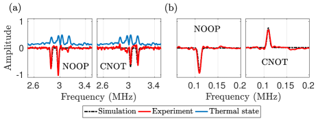
Figure 4: (a) Electron spin spectra for the pulse sequence corresponding to Fig. 3(a) without and with $U_{CNOT}$where $\theta_{y}=\pi$. The thermal state spectra on top are shifted vertically for reference. The electron spin spectra are centered around the detuning frequency 3 MHz. (b) ¹³C spin spectra obtained by the pulse sequence shown in Fig. 3(b) without and with $U_{CNOT}$. The peaks appear at $\nu_{-}$= 0.11 MHz.

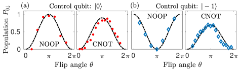
Figure 5: $P_{0\downarrow}$ as a function of $\theta$ corresponding to the pulse sequences shown in Fig. 3(a). The diamonds and solid circles are the experimental data, and the dashed lines are the matching simulations.

As an additional test of the sequence for different input states, we first applied a selective rotation, when $m_{N}=1$ not (d), of $\psi_{0}$ by an angle $\theta_{y}$ to generate the superposition state $\psi_{\theta}=\cos(\theta/2)|0\uparrow\rangle+\sin(\theta/2)|-1\uparrow\rangle$. As shown in Fig. 3(a), we then applied either a NOOP or $U_{CNOT}$. The latter transforms $\psi_{\theta}$ to $\cos(\theta/2)|0\uparrow\rangle-i\sin(\theta/2)|-1\downarrow\rangle$, which is entangled for $\theta\neq n\pi$ with integer $n$. Ideally, the amplitude of the resonance line for the transition $|0\downarrow\rangle$ $\leftrightarrow|1\downarrow\rangle$ not (e) is proportional to the population $P_{0\downarrow}$. We thus determined $P_{0\downarrow}$ and the results, which are shown in Fig. 5, demonstrate the effect of $U_{CNOT}$ for the 2 cases where the control qubit is $|0\rangle$ or $|-1\rangle$. Fig. 5(a) shows $P_{0\downarrow}$ after applying NOOP or $U_{CNOT}$ to $\psi_{\theta}$, as a function of $\theta$ in the absence of the $180_{y}$ operation indicated by the dotted box in Fig. 3(a). This pulse sequence allows us to measure the effect of $U_{CNOT}$ when the electron spin is $|0\rangle$. The curves for both cases are similar since $U_{CNOT}$ does not change the ¹³C state when the electron spin is $|0\rangle$. In Fig. 5(b) we show the effect of $U_{CNOT}$ when the electron spin is $|-1\rangle$. To read out the population of $|-1\downarrow\rangle$, we first applied a $180_{y}$ operation, as shown in Fig. 3(a) and then measured the electron spin FID in $m_{S}=\{0,1\}$. In this case, the $P_{0\downarrow}$ vs $\theta$ curve flipped for $U_{CNOT}$ compared to NOOP, indicating the change of the ¹³C state when the electron is in $|-1\rangle$. By fitting the experimental $P_{0\downarrow}$ with the corresponding theoretical populations for various $\theta$ as shown in Fig. 5, we estimated the experimental infidelity due to $U_{CNOT}$ as $20\%$ not (a).

Discussion.— Our experiments convincingly show that the IC scheme is a very effective approach to implement operations in systems consisting of 3 types of qubits. The advantages of this approach will become even more important as the number of qubits increases. While a full implementation of the approach in large quantum registers is beyond the scope of this paper, we have tested the basic scheme through numerical simulations of gates in multiqubit systems with up to six qubits. The simulations show that the procedure scales relatively favorably with the size of the system not (a). For the 6-qubit system our method to control individual ¹³C spins was efficient as it required 3-4 MW pulses and the total duration was $<30\,\mu$s. The theory Khaneja (2007); Lowenthal (1971) regarding the bounds for the control overhead and the condition to retain efficiency for larger spin systems is explained in not (a).

Conclusion.— We experimentally demonstrated full coherent control i.e, state initialization, gate implementation and detection of the electron-nuclear spin system in the NV center of diamond using the methods of IC. We specifically chose a center with a small hyperfine coupling, some three orders of magnitude weaker than that of the nearest neighbor ¹³C spins. The distance between the electron and ¹³C is $\approx 0.89$ nm not (a). These remote spins are much more abundant than the nearest neighbors and their relaxation times much longer. However, since their coupling to RF fields is also much weaker, direct RF excitation does not lead to efficient control operations. The IC techniques that we have demonstrated allow much faster controls and therefore overall higher fidelity - an essential prerequisite for scalable quantum systems. Specifically, we have implemented a Hadamard gate on ¹³C and a CNOT gate, where the electron is the control qubit and ¹³C the target qubit, using only a small number of MW pulses and delays. The above gate operations targeted the subspace $m_{S}=\{0,-1\}$ and $m_{N}=1$. If we consider the control state of the ¹⁴N, i.e $m_{N}=1$, in the whole space with $m_{N}=\{{0,-1,1}\},$ then our $U_{CNOT}$ is a Toffolli gate in $12$ dimensions. Since the total duration of the pulse sequence was well within the electron coherence time ($T_{2}^{*}\approx 20\mu$s), additional coherence preserving control operations were not required. However, for complex algorithms consisting of many gates, it may be necessary to include DD. While we have implemented this scheme in the diamond NV center at room temperature in a small external magnetic field, it remains applicable over a much wider parameter range and can clearly be adapted to other quantum systems, thus opening the ways for many different implementations of advanced quantum algorithms using indirect control schemes.

Acknowledgments.— This work was supported by the DFG through grants SU 192/34-1 and SU 192/31-1 and by the European Union’s Horizon 2020 research and innovation programme under grant agreement No 828946. The publication reflects the opinion of the authors; the agency and the commission may not be held responsible for the information contained in it. SH thanks Dr T S Mahesh for fruitful discussions on genetic algorithms.

1. NV center system and Bloch Sphere representation of the evolution

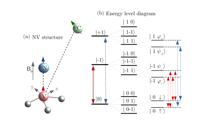
Figure 6: (a) NV center coupled to ¹⁴N and ¹³C spins. The magnetic field $B_{0}$ is aligned along the NV axis in the z direction. (b) The energy level splittings. $\{|0\rangle,|\pm 1\rangle\}$ correspond to electron and ¹⁴N spins, $\{|\uparrow\rangle,|\downarrow\rangle,|\varphi_{\pm}\rangle,|\psi_{\pm}\rangle\}$ correspond to the ¹³C spin. The ESR transitions in the electron spin subspace $m_{S}=$ $\{0,-1\}$, when ¹⁴N spin is in state $m_{N}=1$, are shown by four arrows (red solid lines) in the right-hand part. Similarly, the ESR transitions in the electron spin subspace $m_{S}=$ $\{0,1\}$, when ¹⁴N spin is in state $m_{N}=1$, are shown by two arrows (blue dotted lines) in the right-hand part.

The experiments were carried out on a diamond sample with ¹²C enrichment of $99.995\%$, at room temperature and at a field strength of 14.8 mT. The $T_{2}^{*}$ of the electronic spin that we used in this experiment was about $\approx 20$ $\mu$s. Fig. 6(a) shows the structure of a single NV center coupled to ¹⁴N and ¹³C nuclear spins. The Hamiltonian ${\cal{H}}$ of this system is discussed in the main manuscript. Fig. 6(b) shows the corresponding energy level diagram. The external magnetic field of strength $B_{0}=14.8$ mT lifts the degeneracy of the electronic $|-1\rangle$ and $|+1\rangle$ states. Each of the spin-1 electronic states splits into $\{|0\rangle,|\pm 1\rangle\}$ states of the ¹⁴N spin, which further split into the states $\{|\uparrow\rangle,|\downarrow\rangle,|\varphi_{\pm}\rangle,|\psi_{\pm}\rangle\}$ of the ¹³C spin.

We chose a subspace where the electron spin was in $m_{S}=$ $\{0,-1\}$ and the ¹⁴N spin was in $m_{N}=1$ and referred to this subspace as our system subspace in which we implemented our gate operations. In the system subspace, there are 4 ESR transitions as indicated by the red arrows in Fig. 6(b), since the states $|\varphi_{-}\rangle$ and $|\psi_{-}\rangle$ are linear combinations of $|\uparrow\rangle$ and $|\downarrow\rangle$ states with $\kappa_{-}\approx 86^{\circ}$ as described in Eqs. (1, 2) of the main manuscript.

In the subspace $m_{S}=$ $\{0,1\}$ when $m_{N}=1$, we observe that $\kappa_{+}\approx 10^{\circ}$. Eqs. (1, 2) of the main manuscript indicate that $|\varphi_{+}\rangle\approx|\uparrow\rangle$ and $|\psi_{+}\rangle\approx|\downarrow\rangle$. Therefore only 2 ESR transitions are observed for $m_{S}=$ $\{0,1\}$ and $m_{N}=1$, which correspond to the transitions $|0\uparrow\rangle\leftrightarrow|1\uparrow\rangle$ and |$0\downarrow\rangle\leftrightarrow|1\downarrow\rangle$ as indicated by the blue arrows in Fig. 6(b). This subspace was used to implement the clean-up operation.

Fig. 7(a) is our generic 3-pulse sequence for implementing $U_{H}$ and $U_{CNOT}$. Fig. 7(b,c) shows the resulting trajectories of the electron and ¹³C on the Bloch-sphere.

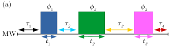
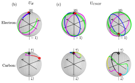
Figure 7: (a) MW pulse sequence to realize $U_{H}$ and $U_{CNOT}$ by IC, at a fixed $\omega_{1}$. The delays $\tau_{i}$, MW pulse durations $t_{i}$ and phases $\phi_{i}$ are the free variables to be optimized. (b, c) Evolution trajectories of electron and ¹³C upon the application of $U_{H}$ and $U_{CNOT}$ for specific initial states. The diamond indicates the initial state and the circle the final state.

2. Analytical form of pulse sequence to map the state $|0\uparrow\rangle$ to $|0\frac{(\uparrow+\downarrow)}{\sqrt{2}}\rangle$

Here, we design an analytical form for the pulse sequence to map the electron-¹³C spin state from an initial state $|0\uparrow\rangle$ to a final state $|0\frac{(\uparrow+\downarrow)}{\sqrt{2}}\rangle$. We choose a generic pulse sequence $(180^{\circ}-\tau_{1}-180^{\circ}-\tau_{2})$, where the $180^{\circ}$ pulse acts on the electron that is resonant with the ESR transition $0\leftrightarrow-1$, and $\tau_{i}$ are delays. The unitary operator for the $180^{\circ}$ pulse is

$$U_{\pi}=e^{-i\pi I_{x}}.$$

During the delays, $\tau_{i}$ with $i=1,2$, the system evolves under the free evolution Hamiltonian ${\cal{H}}_{s}$, where

$${\cal H}_{s}/(2\pi)=(-\nu_{C}-{A_{zz}}/{2})(E_{2}\otimes I_{z})+A_{zz}(I_{z}^{e}\otimes I_{z})+A_{zx}(I_{z}^{e}\otimes I_{x})-{A_{zx}}/{2}(E_{2}\otimes I_{x}).$$ (3)

Here $\nu_{c}=0.158$ MHz is the ¹³C spin Larmor frequency, and $A_{zz}=-0.152$ MHz, $A_{zx}=0.11$ MHz are the hyperfine couplings with the ¹³C spin.

The corresponding evolution operator in the basis $\{|0\uparrow\rangle,|0\downarrow\rangle,|-1\uparrow\rangle,|-1\downarrow\rangle\}$ during $\tau_{i}$ is

$$U_{\tau_{i}}=\begin{bmatrix}e^{i\pi\nu_{C}\tau_{i}}&0&0&0\\ 0&e^{-i\pi\nu_{C}\tau_{i}}&0&0\\ 0&0&\cos(\pi\nu_{-}\tau_{i})+i\cos(\kappa_{-})\sin(\pi\nu_{-}\tau_{i})&i\sin(\kappa_{-})\sin(\pi\nu_{-}\tau_{i})\\ 0&0&i\sin(\kappa_{-})\sin(\pi\nu_{-}\tau_{i})&\cos(\pi\nu_{-}\tau_{i})-i\cos(\kappa_{-})\sin(\pi\nu_{-}\tau_{i})\end{bmatrix},$$

where $\nu_{-}=\sqrt{A_{zx}^{2}+(\nu_{C}+A_{zz})^{2}}$ is the ¹³C spin transition frequency in the $m_{S}=-1$ subspace, and $\kappa_{-}=\tan^{-1}[A_{zx}/(A_{zz}+\nu_{C})]\approx 86^{\circ}$ is the angle between the quantization axis of the ¹³C nuclear spin and the NV axis.

The total propagator for the pulse sequence $(180^{\circ}-\tau_{1}-180^{\circ}-\tau_{2})$ is

$$U=U_{\tau_{2}}U_{\pi}U_{\tau_{1}}U_{\pi}.$$

The state transformation $|0\uparrow\rangle$ $\rightarrow$ $|0\frac{(\uparrow+\downarrow)}{\sqrt{2}}\rangle$, can be written as

$$|0(\uparrow+\downarrow)\rangle\langle 0(\uparrow+\downarrow)|/2=U|0\uparrow\rangle\langle 0\uparrow|U^{\dagger}.$$

By equating the matrix elements $\langle 0\uparrow|U|0\uparrow\rangle$ and $\langle 0\uparrow|U|0\downarrow\rangle$ to $0.5$, we solve for $\tau_{i}$:

$$\tau_{1} = \frac{1}{\pi\nu_{-}}\sin^{-1}(\frac{1}{\sqrt{2}\sin(\kappa_{-})})$$ (4)

$$\tau_{2} = \frac{1}{2\pi\nu_{C}}\cos^{-1}(\frac{\cos(\kappa_{-})}{\sin(\kappa_{-})})$$ (5)

where for our system, $\kappa_{-}\approx 86^{\circ}$, $\nu_{-}=0.11$ MHz and thus $\tau_{1}=2.28$ $\mu$s, $\tau_{2}=1.53$ $\mu$s. $\tau_{1}+\tau_{2}$ sets the lower bound on the pulse sequence duration.

3. State evolution during to the pulse sequence to demonstrate Hadamard gate

We show the details of the state evolution during the pulse sequence in Fig. 2(a) of the main manuscript. The ¹³C spin is initialized into the state

$$\rho_{0}^{c}=\frac{E_{2}}{2}+I_{z}.$$ (6)

$E_{2}$ is a $2\times 2$ identity matrix that does not evolve under any operation, and we track the evolution of $I_{z}$ spin operator at each stage of the pulse sequence Cavanagh et al. (1995). The first Hadamard gate $U_{H}$ transforms $I_{z}$ as:

$$I_{z}\longrightarrow I_{x}$$ (7)

Since, initially the populations of the $m_{S}=-1$ subspace are zero, we concentrate on the evolution of the ¹³C spin state in the $m_{S}=0$ subspace, where the ¹³C spin Hamiltonian is

$${\cal H_{C}}=2\pi\nu_{c}I_{z}.$$ (8)

Here $\nu_{c}$ is the ¹³C spin larmor frequency. During the free precession for a duration $t$, $I_{x}$ evolves as

$$I_{x}\longrightarrow I_{x}\cos(2\pi\nu_{c}t)+I_{y}\sin(2\pi\nu_{c}t)$$ (9)

The second $U_{H}$ takes the above state to $I_{z}\cos(2\pi\nu_{c}t)-I_{y}\sin(2\pi\nu_{c}t).$ Thus the initial state $\rho_{0}^{c}$ goes to the final state

$$\rho^{c}\longrightarrow\frac{E_{2}}{2}+I_{z}\cos(2\pi\nu_{c}t)-I_{y}\sin(2\pi\nu_{c}t)$$ (10)

The last clean-up operation transfers the population from $|0\downarrow\rangle$ to $|1\downarrow\rangle$. Hence, the remaining population of the state $|0\uparrow\rangle$ of equation (10) is $[1+\cos(2\pi\nu_{c}t)]/2$.

4. State determination

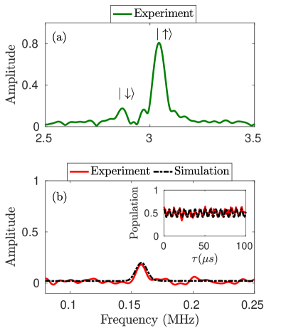
Figure 8: (a) Population determination. ESR spectrum in the subspaces $m_{S}=\{0,1\}$ and $m_{N}=1$ showing $80\%$ population in state $|0\uparrow\rangle$ and $20\%$ population in state $|0\downarrow\rangle$. (b) Coherence determination. The ¹³C spectrum corresponding to the pulse sequence in Fig. 2(a) of the main manuscript without the first $U_{H}$ starting from input state with $80\%$ population in state $|0\uparrow\rangle$ and $20\%$ population in state $|0\downarrow\rangle$.

Fig. 8(a) shows the ESR spectrum of the state $\rho$. It was obtained with the method described in Zhang et al. (2019). The two peaks correspond to the electron spin transitions in the $m_{S}=\{0,1\}$ subspace when the ¹³C spin is in the $|\uparrow\rangle$ and $|\downarrow\rangle$ states, respectively, as indicated in the figure. The area under these spectral lines is proportional to the populations of $|0\uparrow\rangle$ and $|0\downarrow\rangle$. The analysis shows that the populations of $|0\uparrow\rangle$ and $|0\downarrow\rangle$ are $\approx 80\%$ and $\approx 20\%$, respectively.

In order to calculate the coherence of the above state $\rho$, we performed an experiment using the pulse sequence shown in Fig. 2(a) of the main manuscript starting from a state with $\approx 80\%$ and $\approx 20\%$ populations in states $|0\uparrow\rangle$ and $|0\downarrow\rangle$ respectively but omitted the first $U_{H}$ operation. If $\rho$ contains coherence between the states $|0\uparrow\rangle$ and $|0\downarrow\rangle$, then these coherences will evolve during the free evolution time $t$. The second $U_{H}$ converts one component of the coherence to population, and the cleanup operation transfers population from state $|0\downarrow\rangle$ to $|1\downarrow\rangle$. Upon Fourier transformation of the remaining populations of the state $|0\uparrow\rangle$ for variable $t$, we get a frequency domain signal with a peak centered at the ¹³C spin Larmor frequency $\nu_{c}$. Following this argument, we expect no peak at $\nu_{c}$ in the absence of the above coherence terms. The experimental result shown in Fig. 8(b) indicated the presence of a peak at $\nu_{c}$, thereby indicating the presence of coherence between the states $|0\uparrow\rangle$ and $|0\downarrow\rangle$. We determined this coherence by fitting the experimental population of state $|0\uparrow\rangle$ as a function of variable delay $t$ (in Fig. 2(a) of the main manuscript) with the corresponding theoretical input state and by optimizing the coherence amplitudes. We found a coherence of 0.08 and thus our state before the clean-up operation was

$$\rho=\left[{\begin{array}[]{cccc}0.8&0.08&0&0\\ 0.08&0.2&0&0\\ 0&0&0&0\\ 0&0&0&0\end{array}}\right].$$

We further purified this state by a clean-up operation that transferred the population from $|0\downarrow\rangle$ to $|1\downarrow\rangle$ and the coherence between the states $\{|0\uparrow\rangle,|0\downarrow\rangle\}$ to the states $\{|0\uparrow\rangle,|1\downarrow\rangle\}$ Zhang et al. (2018a). This clean-up is a MW pulse sequence $(90_{x}-\tau_{c}-90_{y})$, where $90_{x/y}$ are pulses with rotation angle $90^{\circ}$ about the $x/y$-axis applied to the $m_{S}=0\leftrightarrow 1$ transition with 0.5 MHz Rabi frequency and $\tau_{c}=1/(2|A_{zz}|)$ is the delay between them. After this clean-up, our system subspace spanned by $m_{S}=\{0,-1\}$ and $m_{N}=1$ was in the pure state

$$\psi_{0}=|0\uparrow\rangle$$ (11)

5. Error estimation for CNOT

In this section, we estimate the experimental fidelity of the state after $U_{CNOT}$ using the results from Fig. 5 of the main text. Here Fig. 5(a) corresponds to the case when the electron is in state $|0\rangle$ and thus according to the definition of our gate operation, $U_{CNOT}$ is an identity operation on the ¹³C spin. In the case where the electron is in state $|-1\rangle$, $U_{CNOT}$ flips the ¹³C spin and the results are shown in Fig. 5(b). The theoretical $P_{0\downarrow}$ has the functional form $P_{0\downarrow}(\theta)=[1-\cos\theta]/2$, where the angle $\theta$ parametrises the electron spin input states before applying $U_{CNOT}$. For all $\theta=[0,2\pi]$, we matched the experimental $P_{0\downarrow}$ by multiplying the corresponding theoretical populations by $0.7$ and $0.9$ for $m_{S}=-1$ and $m_{S}=0$ respectively. Thus we observed a $10\%$ signal loss when the electron was in state $|0\rangle$ and a $30\%$ signal loss when electron was in state $|-1\rangle$. The average of these errors is $20\%$ and hence the experimental fidelity of the state after $U_{CNOT}$, which in this case is calculated by measuring $P_{0\downarrow}$, amounted to about $80\%$, in agreement with the results in Fig. 4 of the main manuscript where data are shown for $\theta$ = $\pi$.

6. Gates in Multiqubit systems

Addressing and controlling individual qubits in multiqubit systems is necessary to realize scalable quantum systems. The central electron spin in the NV centers of diamond has potential to be coupled to multiple ¹³C spins, thereby offering a possibility of realizing multiqubit registers. However, the presence of these multiple nuclear spins also is a main contribution to the decoherence and limits the spectral resolution. The duration of the gate operations should therefore not exceed the electron spin coherence time. We here extend our indirect control scheme to the implementation of simple gate operations in multiqubit systems consisting of up to 6 qubits, and check the typical gate durations, the minimum required electron spin coherence time and the control overhead.

Our $n$-qubit system consists of 1 electron spin, 1 ¹⁴N spin and $(n-2)$ ¹³C spins. Here, the operations that we chose are controlled-controlled rotations where the electron spin and the ¹⁴N spin are the control qubits and an individual ¹³C spin is the target qubit. On the remaining spins, the operation should implement a unit operation (NOOP). In the rotating frame of the electron spin with frequency given by $D+\nu_{e}-A_{N}$ (where the notations are defined in the main text), the $n$-qubit system Hamiltonian in the subspaces $m_{S}=\{0,-1\}$ and $m_{N}=1$ can be written as

$$\frac{{\cal H}_{s}^{\otimes n}}{2\pi}=|1_{N}\rangle\langle 1_{N}|\otimes(|0_{e}\rangle\langle 0_{e}|\otimes\sum_{j=1}^{n-2}{\cal H}_{0}^{j}+|-1_{e}\rangle\langle-1_{e}|\otimes\sum_{j=1}^{n-2}{\cal H}_{-1}^{j}),$$ (12)

where $e$ represents the electron, $N$ represents the ¹⁴N, ${\cal H}_{0}^{j}=-\nu_{C}I_{z}^{j}$ and ${\cal H}_{-1}^{j}=-(\nu_{C}+A_{zz}^{j})I_{z}^{j}-A_{zx}^{j}I_{x}^{j}$ are the Hamiltonians for the $j^{\mathrm{th}}$ ¹³C spin. The ¹³C spin Larmor frequency is $\nu_{C}=0.158$ MHz and the chosen hyperfine couplings with the ¹³C spins are listed in Table 2. The simulated spectrum of this Hamiltonian for $n=6$ in the $m_{S}=\{0,-1\}$ and $m_{N}=1$ subspaces is shown in Fig. 9. Thus we see that, a minimum $T_{2}{}^{*}=1/(\pi\delta\nu)\approx 30\,\mu$s, where $\delta\nu$ is the line width of the ESR spectra, is necessary to spectrally address individual ¹³C spins in this system.

$j$	$A_{zz}^{j}$ (MHz)	$A_{zx}^{j}$ (MHz)
1	$A_{zz}^{1}=-0.152$	$A_{zx}^{1}=0.110$
2	$A_{zz}^{2}=(1.5)\cdot A_{zz}^{1}$	$A_{zx}^{2}=(1.5)\cdot A_{zx}^{1}$
3	$A_{zz}^{3}=(2/3)\cdot A_{zz}^{1}$	$A_{zx}^{3}=(2/3)\cdot A_{zx}^{1}$
4	$A_{zz}^{4}=(2.5)\cdot A_{zz}^{1}$	$A_{zx}^{4}=(2.5)\cdot A_{zx}^{1}$

Table 2: Hyperfine couplings $A_{zz}^{j},A_{zx}^{j}$ for a system of four ¹³C spins. $j=1\dots 4$ represents the label for the ¹³C spins.

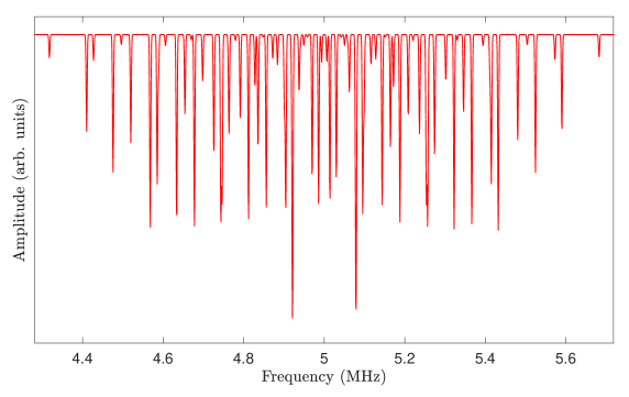
Figure 9: Simulated ESR spectrum of the $n=6$ system, i.e, with all the four ¹³C spins, in the $m_{S}=\{0,-1\}$ and $m_{N}=1$ subspace. The coupling parameters are listed in Table 2 and the detuning frequency was set to 5 MHz.

To design pulse sequences for arbitrary gate operations in multiqubit systems, we extend the optimization protocol for a two qubit system as explained in the main text to that of an $n$ qubit system with the system Hamiltonian ${\cal H}_{s}^{\otimes n}$. The control (MW) Hamiltonian in $m_{N}=1$ is $\omega_{1}[\cos\phi_{i}(s_{x}\otimes E^{\otimes{2^{n-2}}})+\sin\phi_{i}(s_{y}\otimes E^{\otimes{2^{n-2}}}]$ where $\omega_{1}$ is the MW pulse amplitude and $E^{\otimes{m}}$ is the ${2^{m}}\times{2^{m}}$ identity matrix. We show that the controlled-controlled rotations can be implemented using the generic 4 pulse MW pulse sequence as shown in Fig. 10. As explained in the main text, $(\tau_{i},t_{i},\phi_{i})$ are the pulse sequence parameters that are to be optimized to design gates with maximum fidelity with a target unitary operator. The Rabi frequency $\omega_{1}/(2\pi)$ is set to $0.5$ MHz which is used to select the $m_{N}=1$ subspace of the ¹⁴N spin and the pulses are not selective to any of the ¹³C spin transitions.

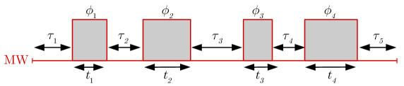
Figure 10: MW pulse sequence to implement controlled-controlled rotations on individual ¹³C spins in muti-qubit systems up to at least $n=6$.

We first simulate a controlled-controlled NOT gate in a $n=4$ system. We separately implement two controlled-controlled NOT gates targeting the $j=1$ spin on two four-qubit systems with different ¹³C spin hyperfine couplings as indicated in Figs. 11(a, b). In Fig. 11(a), the system consists of 1 e, 1 ¹⁴N, and $j=1,2$ carbon spins where the hyperfine coupling with the $j=2$ spin is larger than that of the $j=1$ spin. In Fig. 11(b), we choose a system with 1 e, 1 ¹⁴N, and $j=1,3$ carbon spins where the hyperfine coupling with the $j=3$ spin is weaker than that of the $j=1$ spin. The optimized pulse sequence parameters corresponding to the sequence in Fig. 10 are shown in Table 3. The MW pulse sequence for implementing the controlled-controlled-NOT gate targeting the $j=1$ carbon spin and NOOP on the other carbon spin in either of the two cases were efficiently designed using only 4 MW pulses with total duration of the sequence less than $15\,\mu$s and the theoretical gate fidelities were greater than $0.99$.

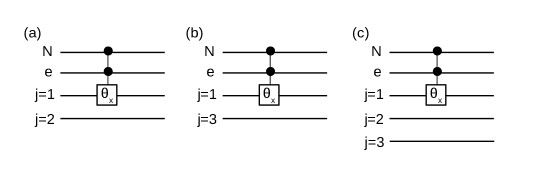
Figure 11: Circuit to implement controlled-controlled-rotations: (a, b) in $n=4$ and (c) in $n=5$. Here $\theta_{x}=e^{-i\theta I_{x}}$.

The $n=5$ system consists of 1 e, 1 ¹⁴N, and $j=1,2,3$ carbon spins. Fig. 11(c) shows the circuit for implementing a selective controlled-controlled-NOT gate targeting only the $j=1$ spin. The corresponding 4-pulse MW pulse sequence parameters are shown in Table 3. This MW pulse sequence implements the above controlled-controlled-NOT gate with a fidelity greater than $0.98$ within a duration of $15\,\mu$s, while simultaneously implementing NOOP on the $j=2,3$ spins.

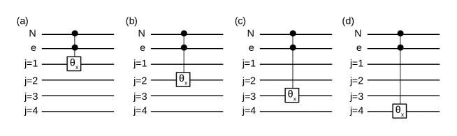
Figure 12: Circuits to implement controlled-controlled-rotations in systems with $n=6$ qubits. Here $\theta_{x}=e^{-i\theta I_{x}}$.

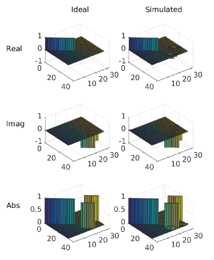
Figure 13: Ideal (right) and simulated (left) unitaries in the $m_{N}=1$ subspace with 1 e and four ¹³C spins using Fig. 12(a). The pulse sequence parameters for the simulated unitary are given in Table 3. In the simulation, $\omega_{1}$ was set to 0.5 MHz and hence, for simplicity, we here show the reduced unitary in the $m_{N}=1$ subspace.

Finally, we consider the $n=6$ qubit case with 1 e, 1 ¹⁴N, and $j=1,2,3,4$ carbon spins. Here we optimize the parameters of the pulse sequence in Fig. 10 for 4 controlled-controlled-rotation operations using the different ¹³C spins as target qubits, as shown in Fig. 12. Table 3 gives the resulting pulse sequence parameters for each of these cases with theoretical gate fidelities ranging from $0.93$ to $0.99$ and total durations ranging from 22-28 $\mu$s. As an example, the form of the ideal and simulated operator in the $m_{N}=1$ subspace corresponding to Fig. 12(a) is shown in Fig. 13.

$n$	$j$	Figure	$\theta$	$\tau_{1}$	$\tau_{2}$	$\tau_{3}$	$\tau_{4}$	$\tau_{5}$	$t_{1}$	$t_{2}$	$t_{3}$	$t_{4}$	$\phi_{1}$	$\phi_{2}$	$\phi_{3}$	$\phi_{4}$	Fidelity	Gate duration ($\mu$s)
$4$	1,2	11(a)	$180^{\circ}$	$1.05$	$1.04$	$1.09$	$1.07$	$4.13$	$2.44$	$1.12$	$0.94$	$1.49$	$61^{\circ}$	$270^{\circ}$	$233^{\circ}$	$90^{\circ}$	$0.991$	$14.4$
$4$	1,3	11(b)	$180^{\circ}$	$0.43$	$0.83$	$0.79$	$1.08$	$2.55$	$2.14$	$1.36$	$1.80$	$1.46$	$298^{\circ}$	$218^{\circ}$	$252^{\circ}$	$90^{\circ}$	$0.996$	$12.4$
$5$	1,2,3	11(c)	$180^{\circ}$	$2.35$	$2.13$	$3.99$	$0.63$	$0.48$	$1.51$	$1.93$	$0.25$	$1.27$	$296^{\circ}$	$315^{\circ}$	$181^{\circ}$	$90^{\circ}$	$0.983$	$14.5$
$6$	1,2,3,4	12(a)	$180^{\circ}$	$4.27$	$2.22$	$0.79$	$3.91$	$6.14$	$1.34$	$1.01$	$1.65$	$1.16$	$206^{\circ}$	$129^{\circ}$	$325^{\circ}$	$90^{\circ}$	0.989	22.5
$6$	1,2,3,4	12(b)	$180^{\circ}$	$4.18$	$7.26$	$1.83$	$1.06$	$6.38$	$2.35$	$0.95$	$0.59$	$0.24$	$182^{\circ}$	$170^{\circ}$	$245^{\circ}$	$90^{\circ}$	0.939	24.8
$6$	1,2,3,4	12(c)	$45^{\circ}$	$5.01$	$2.02$	$2.07$	$3.72$	$5.17$	$0.50$	$1.89$	$0.95$	$0.93$	$276^{\circ}$	$262^{\circ}$	$254^{\circ}$	$90^{\circ}$	0.970	22.3
$6$	1,2,3,4	12(d)	$45^{\circ}$	$4.83$	$3.77$	$4.45$	$2.58$	$6.75$	$1.68$	$1.98$	$1.54$	$0.33$	$176^{\circ}$	$76^{\circ}$	$97^{\circ}$	$90^{\circ}$	0.976	27.9

Table 3: Optimized pulse sequence parameters $(\tau_{i},t_{i},\phi_{i})$ corresponding to the pulse sequence in Fig. 10 to implement controlled-controlled rotations on individual ¹³C spins in the system of size $n$. $j$ indicates the different ¹³C spins that are considered in each case. Each row corresponds to a specific operation as indicated by the Fig. 11 or 12. In all these cases, $\omega_{1}/2\pi=0.5$ MHz. Fidelity represents the theoretically calculated gate fidelities.

Efficiency and comparison with methods based on DD cycles.– The numerically optimized pulse sequence parameters for implemening controlled-controlled rotation gates between specific pairs of qubits in systems with up to $n=6$ qubits show that the indirect control scheme proposed in this work is efficient with only 4 MW pulses and with theoretical gate fidelities ranging from $0.93$ to 0.99. As can be seen in Table 3, the gate durations gradually increase from about $12\,\mu$s for $n=4$ up to $28\,\mu$s for $n=6$. These gate durations will further increase (about $2-3\,\mu$s) if the sequences are made robust with respect to the deviations in $\omega_{1}$. Thus as seen in Table 3, a mimimum $T_{2}^{*}$ of about $30\,\mu$s is necessary to implement controlled-controlled rotations in the $n=6$ system that we considered. Also the control overhead was only 4 MW pulses.

The ¹²C enriched NV sample that we used in our experiments had an electron spin $T_{2}^{*}$ of about $20\,\mu$s and the electron spin coherence time $T_{2}$ for this sample was more than $1.3$ ms Zhang et al. (2018b). This $T_{2}^{*}$ is sufficient for indirect control a single ¹³C spin, but $T_{2}^{*}$ of the electron spin is shorter in crystals with higher ¹³C spin concentration Mizuochi et al. (2009) and the total gate durations will exceed the $T_{2}^{*}$. In such cases, protected quantum gates that are interleaved with the DD pulses Zhang et al. (2014) so as to extend the electron spin $T_{2}^{*}$ beyond $30-100\,\mu$s would assist in coherently addressing the individual nuclear spins in larger spin systems. Also, in our previous work, we showed that one can further improve the fidelity and gate duration by polarizing the ¹⁴N spin instead of working in the subspace $m_{N}=1$ Zhang et al. (2019). For $n>10$, optimizing the pulse sequence parameters using classical computers gets increasingly difficult. Nevertheless, our control scheme could be very useful in cases like Ref. Jiang et al. (2007) where it has been shown that only 5 qubits are sufficient to realize a fully functional quantum repeater node.

Our scheme is efficient for the systems where $\nu_{C}$ is comparable to the hyperfine couplings. In such cases, the difference $\delta$ between the orientation of the quantization axes of the ¹³C spin with the NV axis in $m_{S}=0$ and 1 subspaces is close to $\pi/2$. Following this, the low control overhead of only 4 MW pulses derives from the argument that any rotation in the SO(3) group can be constructed with $\leq m+2$ rotations where $\pi/(m+1)\leq\delta<\pi/m$ Khaneja (2007); Lowenthal (1971). Our scheme holds even for systems where the hyperfine couplings are only a few tens of kHz. This requires that the multiple ¹³C spins under consideration have similar coupling strengths. One can then adjust the external static magnetic field to bring $\nu_{C}$ to a value that is comparable with the couplings. Thus, using this scheme, even very weakly coupled ¹³C spins could be controlled with as few as 3 MW pulses. On the other hand, the indirect control methods based on multiple cycles of DD sequences to achieve a desired nuclear spin rotation work in a different regime where $\nu_{C}\gg(A_{zz},A_{zx})$ Taminiau et al. (2012, 2014). The latter method requires tens to hundreds of MW pulses.

7. Spatial distance between the electron and the ¹³C spin.

The dipolar Hamiltonian between the electron spin with $\gamma_{e}=-1.761\times 10^{11}$ rad $s^{-1}T^{-1}$ and a ¹³C spin with $\gamma_{C}=6.728\times 10^{11}$ rad $s^{-1}T^{-1}$ which is located at a distance $r$ from electron is

$$\mathcal{H}_{d}=\vec{S}\cdot\bar{A}\cdot\vec{I}=-\frac{\mu_{0}}{4\pi}\frac{\gamma_{e}\gamma_{C}h}{r^{3}}[3(\vec{S}.\hat{n})(\vec{I}.\hat{n})-\vec{S}\cdot\vec{I}]$$ (13)

Here $\bar{A}$ if the hyperfine tensor, $\vec{S}$ and $\vec{I}$ are the electron and ¹³C spin operators respectively, $h=6.626\times 10^{-34}\,$Js is Planck’s constant, $\mu_{0}=4\pi\times 10^{-7}\,$Hm^-1 is the magnetic permeability, and $\hat{n}=[n_{x},n_{y},n_{z}]=[\sin(\theta)\cos(\phi),\sin(\theta)\sin(\phi),\cos(\theta)]$ is a unit vector pointing from the electron to the¹³C.

By equating the coefficients of $S_{z}I_{z}$ and $S_{z}I_{x}$ in Eq. 13, we get

$$\begin{split}&A_{zz}=-0.152\,\mathrm{MHz}=[b(r)/2\pi].[3\cos^{2}(\theta)-1].\\ &A_{zx}=0.110\,\mathrm{MHz}=[b(r)/2\pi].[3\sin(\theta)\cos(\theta)]\end{split}$$ (14)

where $b(r)=-\frac{\mu_{0}}{4\pi}\frac{\gamma_{e}\gamma_{C}h}{r^{3}}$ and we have set $\phi=0$ by chosing a reference frame in which the ¹³C is located in the zx-plane. By solving the above equations, we detemined the spatial distance between the electron and ¹³C spin as $r=0.8924$ nm and $\theta=78^{\circ}$.

8. Effects of operations in the ¹⁴N subspaces $m_{N}=\{0,1,-1\}$

In this section, we show that our operations on the electron spin in the subpaces $m_{S}=\{0,-1\}$ and $m_{N}=1$ to implement rotations on the ¹³C spin do not effect the other ¹⁴N subpaces $m_{N}=\{0,-1\}$. To demonstrate this, we compare the thermal state ESR spectrum with the pure state ESR spectrum. As explained in the main text, the pure state is obtained by initializing the electron to state $|0\rangle$ by a 532 nm laser pulse and the¹³C spin is initialized to $|0\rangle$ by the indirect control method. The corresponding MW pulse sequence driving the electron spin consists of 3 pulses followed by a laser pulse of duration 1.1 $\mu$s as explained in the main text. As with the gate implementations for Hadamard and CNOT, the MW pulse amplitude was set to 0.5 MHz and the optimized pulse sequence parameters were $(\tau_{1},\tau_{2},\tau_{3},\tau_{4},t_{1},t_{2},t_{3},\phi_{1},\phi_{2},\phi_{3})=(0,2.09\,\mu s,2.59\,\mu s,0.84\,\mu s,0.52\,\mu s,0.45\,\mu s,1.03\,\mu s,16^{\circ},108^{\circ},90^{\circ})$.

Fig. 14 shows the experimental ESR spectrum for the thermal state (top trace) and pure state (bottom trace) in the $m_{S}=\{0,-1\}$ subspace. The ¹⁴N spin subspaces $m_{N}$ are indicated. In each $m_{N}$ subspace, the thermal spectra have four ESR transitions as explainined in section 1 of this supplementary material. The numbers 1, 2, 3, 4 in the $m_{N}=1$ subspace mark the ESR transitions $|0\uparrow\rangle\leftrightarrow|-1\psi_{-}\rangle$, $|0\uparrow\rangle\leftrightarrow|-1\varphi_{-}\rangle$, $|0\downarrow\rangle\leftrightarrow|-1\psi_{-}\rangle$, $|0\downarrow\rangle\leftrightarrow|-1\varphi_{-}\rangle$ respectively. The pure state spectrum contains only the 2 ESR lines, 1 and 2, in the $m_{N}=1$ subspace but with almost twice the amplitude as in the thermal state, consistent with the subspaces where our gates were designed.

We see that the electron and ¹³C spins were polarized only in the $m_{N}=1$ subspace while the other subspaces. e.g. $m_{N}=0$ retain all the four peaks with comparable spectral amplitudes. This shows that our MW pulse sequences do not affect the ¹³C spins in the other ¹⁴N spin subspaces.

Figure 14: ESR spectrum of the thermal state (top) and the pure state (bottom). Here, the detunig frequency was set to 5 MHz. 1, 2, 3, 4 are the ESR transitions in the $m_{N}=1$ subspace.

References

- Nielsen and Chuang (2002) M. A. Nielsen and I. Chuang, Quantum computation and quantum information (2002).
- Stolze and Suter (2008) J. Stolze and D. Suter, Quantum computing: a short course from theory to experiment (John Wiley & Sons, 2008).
- Gaebel et al. (2006) T. Gaebel, M. Domhan, I. Popa, C. Wittmann, P. Neumann, F. Jelezko, J. R. Rabeau, N. Stavrias, A. D. Greentree, S. Prawer, et al., Nature Physics 2, 408 (2006).
- Neumann et al. (2008) P. Neumann, N. Mizuochi, F. Rempp, P. Hemmer, H. Watanabe, S. Yamasaki, V. Jacques, T. Gaebel, F. Jelezko, and J. Wrachtrup, science 320, 1326 (2008).
- Wrachtrup et al. (2001) J. Wrachtrup, S. Y. Kilin, and A. Nizovtsev, Optics and Spectroscopy 91, 429 (2001).
- Suter and Jelezko (2017) D. Suter and F. Jelezko, Progress in nuclear magnetic resonance spectroscopy 98, 50 (2017).
- Childress et al. (2006) L. Childress, M. G. Dutt, J. Taylor, A. Zibrov, F. Jelezko, J. Wrachtrup, P. Hemmer, and M. Lukin, Science 314, 281 (2006).
- Fuchs et al. (2009) G. Fuchs, V. Dobrovitski, D. Toyli, F. Heremans, and D. Awschalom, Science p. 1181193 (2009).
- Balasubramanian et al. (2009) G. Balasubramanian, P. Neumann, D. Twitchen, M. Markham, R. Kolesov, N. Mizuochi, J. Isoya, J. Achard, J. Beck, J. Tissler, et al., Nature materials 8, 383 (2009).
- Maurer et al. (2012) P. C. Maurer, G. Kucsko, C. Latta, L. Jiang, N. Y. Yao, S. D. Bennett, F. Pastawski, D. Hunger, N. Chisholm, M. Markham, et al., Science 336, 1283 (2012).
- Herbschleb et al. (2019) E. Herbschleb, H. Kato, Y. Maruyama, T. Danjo, T. Makino, S. Yamasaki, I. Ohki, K. Hayashi, H. Morishita, M. Fujiwara, et al., Nature communications 10, 1 (2019).
- Bradley et al. (2019) C. Bradley, J. Randall, M. Abobeih, R. Berrevoets, M. Degen, M. Bakker, M. Markham, D. Twitchen, and T. Taminiau, Physical Review X 9, 031045 (2019).
- Gali et al. (2008) A. Gali, M. Fyta, and E. Kaxiras, Physical Review B 77, 155206 (2008).
- Meiboom and Gill (1958) S. Meiboom and D. Gill, Review of scientific instruments 29, 688 (1958).
- Uhrig (2007) G. S. Uhrig, Physical Review Letters 98, 100504 (2007).
- Zhang and Suter (2015) J. Zhang and D. Suter, Physical review letters 115, 110502 (2015).
- Van der Sar et al. (2012) T. Van der Sar, Z. Wang, M. Blok, H. Bernien, T. Taminiau, D. Toyli, D. Lidar, D. Awschalom, R. Hanson, and V. Dobrovitski, Nature 484, 82 (2012).
- Suter and Álvarez (2016) D. Suter and G. A. Álvarez, Rev. Mod. Phys. 88, 041001 (2016), URL http://link.aps.org/doi/10.1103/RevModPhys.88.041001.
- Zhang et al. (2014) J. Zhang, A. M. Souza, F. D. Brandao, and D. Suter, Physical review letters 112, 050502 (2014).
- Jelezko et al. (2004) F. Jelezko, T. Gaebel, I. Popa, M. Domhan, A. Gruber, and J. Wrachtrup, Physical Review Letters 93, 130501 (2004).
- Shim et al. (2013) J. Shim, I. Niemeyer, J. Zhang, and D. Suter, Physical Review A 87, 012301 (2013).
- Rao and Suter (2016) K. R. K. Rao and D. Suter, Physical Review B 94, 060101 (2016).
- Maze et al. (2008) J. Maze, J. Taylor, and M. Lukin, Physical Review B 78, 094303 (2008).
- Khaneja (2007) N. Khaneja, Physical Review A 76, 032326 (2007).
- Wang et al. (2017) F. Wang, Y.-Y. Huang, Z.-Y. Zhang, C. Zu, P.-Y. Hou, X.-X. Yuan, W.-B. Wang, W.-G. Zhang, L. He, X.-Y. Chang, et al., Physical Review B 96, 134314 (2017).
- Zhang et al. (2011) Y. Zhang, C. A. Ryan, R. Laflamme, and J. Baugh, Physical review letters 107, 170503 (2011).
- Hodges et al. (2008) J. S. Hodges, J. C. Yang, C. Ramanathan, and D. G. Cory, Physical Review A 78, 010303 (2008).
- Cappellaro et al. (2009) P. Cappellaro, L. Jiang, J. Hodges, and M. D. Lukin, Physical review letters 102, 210502 (2009).
- Taminiau et al. (2012) T. Taminiau, J. Wagenaar, T. Van der Sar, F. Jelezko, V. V. Dobrovitski, and R. Hanson, Physical review letters 109, 137602 (2012).
- Aiello and Cappellaro (2015) C. D. Aiello and P. Cappellaro, Physical Review A 91, 042340 (2015).
- Taminiau et al. (2014) T. H. Taminiau, J. Cramer, T. van der Sar, V. V. Dobrovitski, and R. Hanson, Nature nanotechnology 9, 171 (2014).
- not (a) See the Supplemental Material for details of NV center system, Bloch Sphere representation of the gates, initial state determination, error estimation for CNOT, gates in multiqubit systems, spatial distance between the electron and the 13C, effects of operations on the 14N used in this work, which includes Refs. Cavanagh et al. (1995); Jiang et al. (2007); Lowenthal (1971); Zhang et al. (2018b); Mizuochi et al. (2009).
- not (b) These operations are written in the computational basis states which is related to the energy eigenbasis by a transformation matrix .
- Mitchell (1998) M. Mitchell, An Introduction to Genetic Algorithms (MIT Press, Cambridge, MA, USA, 1998), ISBN 0262631857.
- Zhang et al. (2019) J. Zhang, S. S. Hegde, and D. Suter, Physical Review Applied 12, 064047 (2019).
- Zhang et al. (2018a) J. Zhang, S. S. Hegde, and D. Suter, Physical Review A 98, 042302 (2018a).
- not (c) Here the hard operation refers to the operation in subspace and . The corresponding Rabi frequency is 8MHz.
- Cavanagh et al. (1995) J. Cavanagh, W. J. Fairbrother, A. G. Palmer III, and N. J. Skelton, Protein NMR spectroscopy: principles and practice (Elsevier, 1995).
- not (d) If operation is a hard pulse as before, then for any value of not equal to integral multiple of , this pulse creates electron spin coherence in subspaces that evolve during the gate operations implemented in the system subspace. For simplicity, we here chose operation as selective pulse subjected to with Rabi frequency 0.5 MHz as we vary value.
- not (e) Unlike the 4 ESR peaks in subspace, the ESR spectra in subspace has only two observable resonance peaks, where one peak corresponds to total population of state and the other peak corresponds to total population of state [see Ref. 31].
- Lowenthal (1971) F. Lowenthal, The Rocky Mountain Journal of Mathematics 1, 575 (1971).
- Jiang et al. (2007) L. Jiang, J. M. Taylor, A. S. Sørensen, and M. D. Lukin, Physical Review A 76, 062323 (2007).
- Zhang et al. (2018b) J. Zhang, S. Saha, and D. Suter, Physical Review A 98, 052354 (2018b).
- Mizuochi et al. (2009) N. Mizuochi, P. Neumann, F. Rempp, J. Beck, V. Jacques, P. Siyushev, K. Nakamura, D. Twitchen, H. Watanabe, S. Yamasaki, et al., Physical review B 80, 041201 (2009).
Supplemental Material for “Efficient quantum gates for individual nuclear spin qubits by indirect
control”
Swathi S. Hegde, Jingfu Zhang, and Dieter Suter
Fakultät Physik, Technische Universität Dortmund,
D-44221 Dortmund, Germany