Mean velocity and effective diffusion constant for translocation of biopolymer chains across membrane

Abstract

Chaperone-assisted translocation through a nanopore embedded in membrane holds a prominent role in the transport of biopolymers. Inspired by classical Brownian ratchet, we develop a theoretical framework characterizing such translocation process through a master equation approach. In this framework, the polymer chain, provided with reversible binding of chaperones, undergoes forward/backward diffusion, which is rectified by chaperones. We drop the assumption of timescale separation and keep the length of a polymer chain finite, both of which happen to be the key points in most of the previous studies. Our framework makes it accessible to derive analytical expressions for mean translocation velocity and effective diffusion constant in stationary state, which is the basis of a comprehensive understanding towards the dynamics of such process. Generally, the translocation of polymer chain across membrane consists of three subprocesses: initiation, termination, and translocation of the main body part of a polymer chain, where the translocation of the main body part depends on the binding/unbinding kinetics of chaperones. That is the main concern of this study. Our results show that the increase of forward/backward diffusion rate of a polymer chain and the binding/unbinding ratio of chaperones both raise the mean translocation velocity of a polymer chain, and roughly speaking, the dependence of effective diffusion constant on these two factors achieves similar behavior.

I Introduction

Translocation across membranes is ubiquitous during or after the synthesis of biopolymers. A typical example is the precursor proteins destined for the matrix of mitochondria or the endoplasmic reticulum Walfter2002The ; Rapoport2007Protein ; Neupert2015A . Additional examples, including the export of RNA across nuclear membranes in eukaryotic cells Santos1998Nuclear ; Schatz1996Common and the viral injection of DNA into a host MolecularBiologyCell ; Liu2014viral , both involve the translocation through nanoscopic pores embedded in biological membranes. Besides, new evidence indicates that the uptake of long DNA molecule concerns linear passage through nuclear pore complex Salman2001Kinetics . Despite the lack of a membrane-bound nucleus or any membrane-bound organelle, the DNA of bacteria travels across cell envelope through narrow constrictions during the process of horizontal gene transfer Allemand2010Bacterial ; Burton2010Membrane ; Chen2005Ins , such as transformation Chen2004DNA , which is responsible for the adaptive evolution of bacteria. Similar transport mechanisms have also been reported in the biotechnology of drug delivery Holowka2007Polyarginine and rapid DNA sequencing as well Turner2002Confinement .

In recent decades, wide attention has been attracted to understanding the mechanism of such crucial biological process. Pioneering work has established various mechanistic understandings of what induces the directional movement of biopolymers through narrow pores. One important driving force is external electric field across the membrane as demonstrated by experiments in vitro Kasianowicz1996Chara ; Meller2000Rapid and extensive theoretical analysis Sung1996Polymer ; Meller2001Voltage ; Corsi2006Field . Considering there is usually no strong enough electric field in living cells, the other mechanism, Brownian ratchet, suggests pure random thermal diffusion is rectified by chemical asymmetry between the cis and trans sides of the membrane, giving rise to a directional motion Simon1992What ; Peskin1993Cellular . That is exactly the main interest of this paper. A typical case, particularly for proteins, is that the binding of chaperones to the translocating polymer on the trans side of a membrane prohibits the polymer chain’s backward diffusion to the cis side, thus leading to the directional translocation Elston2000Models ; Matlack1998Protein ; Walfter2002The . This mechanism appears to be confirmed on the basis of empirical data for the transport of prepro-$\alpha$ factor into the lumen of endoplasmatic reticulum, where prepro-$\alpha$-factor is regarded as protein and BiP serves as a chaperone molecule Matlack1999BiP . Recent progress on the kinetic of uptake of DNA also provides evidence for analogous mechanism Hepp2016Kinetics .

Quantitative investigations devoted to chaperone-assisted transcription mainly focus on the dynamic properties of the system, with theoretical explorations set up mostly through a continuous space and time description Simon1992What ; Peskin1993Cellular ; Roya2003What . Such continuum models can work effectively in the limit that chaperones are of much lager size compared with the translocating polymer. However, this may become unrealistic in living cells.

Other studies contribute to translocation process of such structure usually through discrete master equations. Early results based on one-dimensional master equations are derived on the simple assumption that both the attachment and the detachment of corresponding chaperones are much faster than the translocation rate, leaving the state of individual sites drawn from the stationary distribution Ambj2004Chaperone ; Ambj2005Directed . Dropping this approximation, a more general discrete model is then proposed in D2007Exact , where the translocating polymer is represented by a one-dimensional lattice of infinite length and an analytical expression for the transcription velocity is obtained mathematically. In Krapivsky2010Fluctuations , extensive analysis was carried out on this model to determine diffusion constant and even higher cumulants of the translocated length, while the same process is discussed from the viewpoint of first-passage time in Abdolvahab2011First . All these three models enjoy a common feature, that is they always keep track of the state of each binding site having been translocated to the target region. This approach, although ideal, seems not feasible, especially for long polymer chains, since the space of states shall experience an explosion as the number of binding sites grows. In this sense, such model makes a difference merely on the numerical simulation side, even if explicit expressions for some dynamic quantities can be obtained. To avoid this issue, a fresh study on this problem set up a modified translocation ratchet model involving the state of only a few binding sites Uhl2018Force . Although a model is proposed dropping the key assumption of timescale separation between the binding/unbinding process of chaperones and the forward/backward diffusion process, analytical results become no longer accessible. Meanwhile, the length of a particular polymer chain is always assumed to be infinite on both side of the membrane in this model, which is not quite appropriate.

In this paper, based on the classical Brownian ratchet, a general framework describing the chaperone-assisted translocation of a polymer chain across membrane is provided. Since the binding/unbinding kinetics of chaperones might have a sizable effect on the dynamics of translocation process, as addressed in previous work D2007Exact ; Krapivsky2010Fluctuations , the state of binding sites locating just behind the membrane, i.e., whether it is bound with a chaperone, is taken into account explicitly in our model. Moreover, the usual assumption of infinite length of polymer chain is also removed. That is to say, the number of binding sites of a particular polymer chain, or say the length of polymer chain, is assumed to be finite in our model. Through a scheme similar to that in Derrida1983Velocity , the mean velocity and effective diffusion constant of polymer translocation are obtained explicitly.

This paper is organized as follows. On the concept of Brownian ratchet, a model describing the process of polymer translocation across membrane is introduced in Sec. II. How this model works will be explained in detail with coupled master equations. In Sec. III, we deduce analytical expressions for mean translocation velocity and effective diffusion constant. To show basic properties of the translocation process, numerical results are presented in Sec. IV. Finally, we summary our results briefly in Sec. V.

II Theoretical description of polymer translocation across membrane through a nanopore

During the translocation across membrane, a polymer chain moves stochastically to either side of the pore embedded in the membrane, which is the only possible gate that polymers can finally climb out. Chaperones are assumed to exist in the target region only. Once the binding site of polymer chain adjacent to the pore is occupied with a chaperone, the polymer chain will then be prevented to move backward through the pore due to the large relative size of a chaperone with respect to the diameter of the narrow pore.

A polymer chain of finite length is represented as a one-dimensional lattice with $N$ binding sites, labeled as $1,2,\cdots,N$. For convenience, the distance between each two neighboring binding sites is normalized to one. If we take the polymer chain as the reference frame, the process of translocation of a polymer chain across membrane through a pore can be regarded as the membrane’s stochastic motion along a one-dimensional lattice. Besides, we represent the membrane as a wall perpendicular to the polymer chain for simplicity. If the wall is standing at site $k$ and the previous site, labeled as $k-1$, remains unoccupied, the wall may hop stochastically either forward to the next site $k+1$ with rate $\omega_{f_{0}}$, or backward to site $k-1$ with rate $\omega_{b}$. Otherwise, if the site $k-1$ is occupied with a chaperone, the wall will have no choice but to hop forward stochastically by one step and the corresponding rate is denoted as $\omega_{f_{1}}$. In summary, the stochastic motion of membrane along polymer chain can be divided into two categories, one is the usual diffusion process with possible forward and backward hopping and the other is the rectified diffusion with possible forward hopping alone, since the backward hopping is blocked by chaperones. In this sense, our model can be regarded as a Brownian ratchet translocation model.

We assume that chaperones can stochastically bind to any unoccupied site behind the wall with rate $\omega_{a}$. At the same time, any attached chaperone can detach from its binding sites at random as well, where the detachment rate is denoted as $\omega_{d}$. It’s easy to find that the dynamics of a translocation process depend on the states of all the binding sites of the polymer chain behind the wall. An ideal model, therefore, should include the states of all these binding sites, i.e., whether it is occupied by some chaperone or not. However, keeping all these states in the model explicitly will make further theoretical analysis inaccessible, especially for long polymer chains, since the state space grows exponentially with the number of binding sites.

Taking this into consideration, we assume that the binding sites two units or more away from the wall have sufficient time to reach equilibrium, and the probability of staying unoccupied thereby comes to $q=\omega_{d}/(\omega_{a}+\omega_{d})$. Actually, the binding/unbinding kinetics of chaperones is much faster than the forward/backward diffusion process of a polymer chain’s translocation across the membrane. The ratio of their timescales lies around $1/300$ Ulrich2002Physical , which makes the assumption plausible therefore.

Our model characterizing the stochastic translocation of a polymer chain across membrane, or equivalently the stochastic motion of a wall along a one-dimensional lattice with length $N$ is depicted in Fig. 1. For $k=2,\dots,N$, we denote $P_{k,0}$ and $P_{k,1}$ as the probability that the wall stands at site $k$ with the previous site $k-1$ unoccupied or occupied with a chaperone respectively, see Fig. 1(a, b). The first site of a polymer chain is labeled as $1$, and the corresponding probability that the wall stands at this site, site $1$, is denoted as $P_{1}$. Additionally, we denote $P_{0}$ as the probability that none of the sites of a polymer chain is passing through the pore, i.e., the nanopore of the membrane is vacant. In other words, $P_{0}$ is the probability that a polymer chain has just accomplished its translocation, and a new translocation process has not started yet.

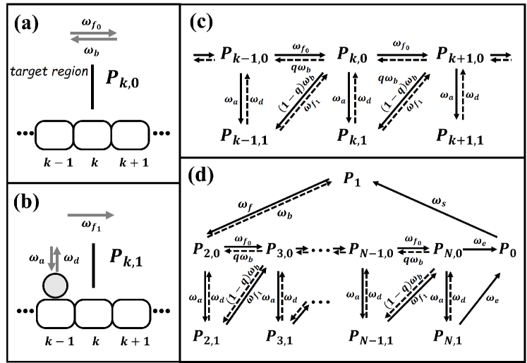
Figure 1: Schematic depiction of the chaperone-assisted translocation of polymer chain across membrane. (a) and (b) depict the two possible states included in our model, that is whether the last site transferred is unoccupied or occupied with a chaperone. The corresponding probabilities are denoted as $P_{k,0}$ and $P_{k,1}$ respectively. Here, the linear polymer molecule is represented by a one-dimension lattice, the bar stands for the moving wall (membrane) and the circle is for a chaperone. Target region of polymer chain is on the left side of the wall. (c) provides a detailed description of possible transitions around a main body site $k$ ($2\leq k\leq N-1$) and related transition rates included in master equations, while (d) shows the transitions around boundary sites $1$ and $N$.

Since chaperones just exist in the target region, only the sites behind the wall are permitted to be bound with chaperones. Then, the wall, standing at site $k$ currently, can always move forward stochastically to the next site $k+1$, while it gets quite different for backward motion. If the site $k-1$ is unoccupied, the wall at site $k$ can also stochastically move backward to site $k-1$ with rate $\omega_{b}$. However, if the site $k-1$ is occupied with a chaperone, the backward motion of the wall at site $k$ will be blocked. That is to say, the forward motion of the wall standing at site $k$ may depend on the state of site $k-1$. To state a general case, the forward hopping rate of the wall is denoted differently, where $\omega_{f_{0}}$ and $\omega_{f_{1}}$ match the cases that site $k-1$ stays in unoccupied and occupied state.

To picture the site-by-site translocation process, we can still imagine a wall standing at some main body site, labeled as $k$. As described in the beginning of this section,the probability that site $k-2$ stays in unoccupied state is $q$, with this site reaching the equilibrium of binding/unbinding kinetics. Based on sustained translocation process, we establish a one-dimensional system of period $l$, where one period indicates a complete transfer of one identical polymer chain. Then, master equations of probabilities $P_{k,0}$ and $P_{k,1}$ in the main body of a lattice, i.e., $k=3,\cdots,N-1$ are given by

$$\frac{\partial P_{k,0}(l,t)}{\partial t}= q\omega_{b}P_{k+1,0}(l,t)+\omega_{f_{0}}P_{k-1,0}(l,t)+\omega_{f_{1}}P_{k-1,1}(l,t)$$

$$+\omega_{d}P_{k,1}(l,t)-(\omega_{b}+\omega_{a}+\omega_{f_{0}})P_{k,0}(l,t)\,,$$ (1)

$$\frac{\partial P_{k,1}(l,t)}{\partial t}= (1-q)\omega_{b}P_{k+1,0}(l,t)+\omega_{a}P_{k,0}(l,t)-(\omega_{d}+\omega_{f_{1}})P_{k,1}(l,t)\,.$$ (2)

See Fig. 1(c) for the schematic depiction.

Since site $1$ is the starting point of translocation process (see Fig. 1(d)), there is no lattice site behind the wall if it stands at site $1$, indicating that no chaperone can be attached to the polymer chain when $k=1$. Thus, the forward hopping rate of the wall at site $k=1$ may be different from both $\omega_{f_{0}}$ and $\omega_{f_{1}}$. Therefore, a different notation $\omega_{f}$ is used to denote the forward hopping rate of the wall for $k=1$. As schematically depicted in Fig. 1(d), Eq. (2) still holds for $k=2$ while Eq. (II) should be modified as

$$\frac{\partial P_{2,0}(l,t)}{\partial t}=q\omega_{b}P_{3,0}(l,t)+\omega_{f}P_{1}(l,t)+\omega_{d}P_{2,1}(l,t)-(\omega_{b}+\omega_{a}+\omega_{f_{0}})P_{2,0}(l,t)\,.$$ (3)

When it comes to the boundary sites, things get different. As discussed above, we use $P_{0}$ to denote the probability that the system stays in the interval between two translocation processes of separate polymer chains, and in this state, the wall can be regarded to stand at a fictitious site $0$. Translocation starts with rate $\omega_{s}$ when the wall binds to the initial lattice site $1$ of a polymer chain, or we say the wall jumps from the fictitious site $0$ to site $1$ with rate $\omega_{S}$. Similarly, it is when the wall hops forward from the terminal site $N$ to the fictitious site $0$ with rate $\omega_{e}$ that the translocation of a polymer chain comes to an end. Also see Fig. 1(d) for a schematic depiction. Based on this scenario, the master equation for probability $P_{1}$ is as follows,

$$\frac{\partial P_{1}(l,t)}{\partial t}=\omega_{s}P_{0}(l,t)+\omega_{b}P_{2,0}(l,t)-\omega_{f}P_{1}(l,t)\,.$$ (4)

Similarly, probabilities $P_{N,0}$ and $P_{N,1}$ are governed by

$$\frac{\partial P_{N,0}(l,t)}{\partial t} =\omega_{f_{0}}P_{N-1,0}(l,t)+\omega_{f_{1}}P_{N-1,1}(l,t)+\omega_{d}P_{N,1}-(\omega_{b}+\omega_{a}+\omega_{e})P_{N,0}(l,t)\,,$$ (5)

$$\frac{\partial P_{N,1}(l,t)}{\partial t} =\omega_{a}P_{N,0}-(\omega_{d}+\omega_{e})P_{N,1}(l,t)\,.$$ (6)

Once a polymer chain has been transferred to the target region completely, the translocation process enters into a pause state, where the wall will wait until it walks onto another polymer chain, that is when another polymer chain enters into the nanopore. With Fig. 1(d), the probability $P_{0}$ satisfies

$$\frac{\partial P_{0}(l,t)}{\partial t}=\omega_{e}[P_{N,0}(l-1,t)+P_{N,1}(l-1,t)]-\omega_{s}P_{0}(l,t)\,.$$ (7)

Hence, we have set up a system of $2N$ states, where the translocation of a polymer chain across a nanopore of membrane is mapped into the motion of a wall through a one-dimensional lattice in terms of relative motion.

III Expressions for Mean Velocity and Effective Diffusion Constant

In this section, we will follow the main idea of Derrida1983Velocity ; Kolomeisky2005Dynamic to realize analytical expressions for mean velocity and effective diffusion constant of translocation of polymer chains across membrane in the stationary-state limit i.e., $t\rightarrow\infty$. We begin with a general expression for the mean location of the wall, which is

$$\langle x(t)\rangle=\sum_{l=-\infty}^{+\infty}\sum_{k=0}^{N}(k+Nl)P_{k}(l,t)\,.$$ (8)

That is to say, if we assume the length of each biopolymer chain equals $N$, each translocation period will add $N$ units to the accumulated distance that the wall travels, since hopping away from a polymer chain (translocation termination, from site $N$ to fictitious site $0$), or stepping into a new period (translocation initiation, from fictitious site $0$ to site $1$), does not increase the total distance that the wall travels. Note that, in Eq. (8) $P_{k}(l,t):=P_{k,0}(l,t)+P_{k,1}(l,t)$ for $2\leq k\leq N$, is the probability that the wall stands at site $k$ of the $l-$th polymer at time $t$(see Fig. 1). We now define a few auxiliary functions for each state concerned, which are shown as

$$B_{k}(t)=\sum_{l=-\infty}^{+\infty}P_{k,0}(l,t),\quad C_{k}(t)=\sum_{l=-\infty}^{+\infty}(k+Nl)P_{k,0}(l,t)\,,$$ (9)

$$\widetilde{B}_{k}(t)=\sum_{l=-\infty}^{+\infty}P_{k,1}(l,t)\,,\quad\widetilde{C}_{k}(t)=\sum_{l=-\infty}^{+\infty}(k+Nl)P_{k,1}(l,t)\,.$$ (10)

Notably, functions in Eq. (9) are defined for index $k$ such that $0\leqslant k\leqslant N$ whereas those in Eq. (10) are defined for $2\leqslant k\leqslant N$ only. Here, for convenience, we assume $P_{k,0}(l,t)=P_{k}(l,t)$ for $k=0,1$ in Eq. (9). Generalizing the original Derrida’s method Derrida1983Velocity ; Kolomeisky2005Dynamic , we propose the following ansatz in the stationary-state limit when time goes infinity.

$$B_{k}(t)\rightarrow b_{k},\quad\widetilde{B}_{k}(t)\rightarrow\widetilde{b}_{k}\,,$$ (11)

$$C_{k}(t)\rightarrow a_{k}t+T_{k},\quad\widetilde{C}_{k}(t)\rightarrow\widetilde{a}_{k}t+\widetilde{T}_{k}\,,$$ (12)

where the range of index $k$ is the same as that in Eqs. (9, 10). Obviously, all these $b_{k}\,$s together with $\widetilde{b}_{k}\,$s are governed by the normalizing condition

$$b_{0}+b_{1}+\sum_{k=2}^{N}(b_{k}+\widetilde{b}_{k})=1\,,$$ (13)

since $b_{k}$ (or $\widetilde{b}_{k}$) gives the probability of finding the wall at a specific state at large time $t$.

In the stationary-state limit, which means $B_{k}(t)\rightarrow b_{k}$, $\widetilde{B}_{k}\rightarrow\widetilde{b}_{k}$ and $\mathrm{d}B_{k}/\mathrm{d}t=0$, $\mathrm{d}\widetilde{B}_{k}/\mathrm{d}t=0$ when $t\rightarrow\infty$, master equations given in Sec. II are transformed into

$$\begin{split}0=&-\omega_{s}b_{0}+\omega_{e}(b_{N}+\widetilde{b}_{N})\,,\\ 0=&\omega_{s}b_{0}-\omega_{f}b_{1}+\omega_{b}b_{2}\,,\\ 0=&\omega_{f}b_{1}-(\omega_{b}+\omega_{f_{0}}+\omega_{a})b_{2}+\omega_{d}\widetilde{b}_{2}+q\omega_{b}b_{3}\,,\\ 0=&\omega_{f_{0}}b_{k-1}+\omega_{f_{1}}\widetilde{b}_{k-1}-(\omega_{a}+\omega_{f_{0}}+\omega_{b})b_{k}+\omega_{d}\widetilde{b}_{k}+q\omega_{b}b_{k+1}\,,\quad(k=3,\cdots,N-1)\,,\\ 0=&\omega_{f_{0}}b_{N-1}+\omega_{f_{1}}\widetilde{b}_{N-1}-(\omega_{a}+\omega_{e}+\omega_{b})b_{N}+\omega_{d}\widetilde{b}_{N}\,,\\ 0=&\omega_{a}b_{k}-(\omega_{d}+\omega_{f_{1}})\widetilde{b}_{k}+(1-q)\omega_{b}b_{k+1}\,,\quad(k=2,3,\cdots,N-1)\,,\\ 0=&\omega_{a}b_{N}-(\omega_{d}+\omega_{e})\widetilde{b}_{N}\,.\end{split}$$ (14)

The last two equations yield

$$\widetilde{b}_{k}=\left\{\begin{split}&(\omega_{d}+\omega_{e})^{-1}\omega_{a}b_{k}\,,\quad(k=N)\,,\\ &(\omega_{d}+\omega_{f_{1}})^{-1}[\omega_{a}b_{k}+(1-q)\omega_{b}b_{k+1}]\,,\quad(k=2,3,\cdots,N-1)\,.\end{split}\right.$$ (15)

The substitution of Eq. (15) into Eq. (14) leads to a recurrence

$$Rb_{N}-Sb_{N-1}=\cdots=Rb_{k}-Sb_{k-1}=\cdots=Rb_{3}-Sb_{2}=\omega_{b}b_{2}-\omega_{f}b_{1}=-\omega_{s}b_{0}\,,$$ (16)

where

$$R=\omega_{b}\frac{\omega_{d}+q\omega_{f_{1}}}{\omega_{d}+\omega_{f_{1}}}\quad\text{and}\quad S=\omega_{f_{0}}+\frac{\omega_{a}\omega_{f_{1}}}{\omega_{d}+\omega_{f_{1}}}\,.$$

Eq. (16) means that the probability fluxes between each two neighboring effective sites $k-1$ and $k$ remain constant in steady state.

Considering the stationary state for boundary sites, i.e. the first equation and the last equation in Eq. (14), we have

$$b_{N}=\left[\omega_{e}+\frac{\omega_{a}\omega_{e}}{\omega_{d}+\omega_{e}}\right]^{-1}\omega_{s}b_{0}\equiv K\omega_{s}b_{0}\,.$$ (17)

The recurrence given in Eq. (16) along with Eq. (17) yields a general expression for $b_{k}$,

$$\begin{split}b_{k}&=\left[\widetilde{S}^{k-N}[K-(S-R)^{-1}]+(S-R)^{-1}\right]\omega_{s}b_{0}\,,\quad(k=2,\cdots,N)\,,\\ b_{1}&=\omega_{f}^{-1}(\omega_{b}b_{2}+\omega_{s}b_{0})\,,\end{split}$$ (18)

where $\widetilde{S}\equiv S/R$. Thus, all of $b_{k}\,$s and $\widetilde{b}_{k}\,$s are determined by $\omega_{s}b_{0}$, which is the probability flux exactly. See Eq. (16). With the normalizing condition given in Eq. (13), we obtain

$$\omega_{s}b_{0}=\left[W_{1}+W_{2}\widetilde{S}^{2-N}+W_{3}(N-1)\right]^{-1}\,,$$ (19)

where

$$W_{1}=\frac{1}{\omega_{s}}+\frac{1}{\omega_{f}}+K(\frac{\omega_{a}}{\omega_{d}+\omega_{e}}-\frac{\omega_{a}}{\omega_{d}+\omega_{f_{1}}})+\frac{U}{S-R}+M\frac{S}{S-R}(K-\frac{1}{S-R}),$$

$$W_{2}=\left(K-\frac{1}{S-R}\right)\left(U-\frac{M}{\widetilde{S}-1}\right)\quad\text{and}\quad W_{3}=\frac{M}{S-R}\,,$$

with

$$M=1+\frac{\omega_{a}}{\omega_{d}+\omega_{f_{1}}}+\frac{(1-q)\omega_{b}}{\omega_{d}+\omega_{f_{1}}}\quad\text{and}\quad U=\frac{\omega_{b}}{\omega_{f}}-\frac{(1-q)\omega_{b}}{\omega_{d}+\omega_{f_{1}}}\,.$$

So far, $b_{0}$ has been obtained explicitly as a function of all constant rates. So do $b_{k}\,$s and $\widetilde{b}_{k}\,$s. See Eqs. (18, 19) and Eq. (15).

Let’s return to the ansatz given in Eq. (12) to derive explicit expressions for $a_{k}\,$s, $\widetilde{a}_{k}\,$s, $T_{k}\,$s and $\widetilde{T}_{k}\,$s. With the definitions of $C_{k}(t)$ and $\widetilde{C}_{k}(t)$ (see Eq. (9) and Eq. (10)) as well as the master equations presented in Sec. II, it is easy to show that $C_{k}(t)$ and $\widetilde{C}_{k}(t)$ satisfy

$$\frac{\mathrm{d}C_{0}}{\mathrm{d}t}(t)= -\omega_{s}C_{0}+\omega_{e}(C_{N}+\widetilde{C}_{N})\,,$$ (20)

$$\frac{\mathrm{d}C_{1}}{\mathrm{d}t}(t)= \omega_{s}C_{0}-\omega_{f}C_{1}+\omega_{b}C_{2}+\omega_{s}B_{0}-\omega_{b}B_{2}\,,$$

$$\frac{\mathrm{d}C_{2}}{\mathrm{d}t}(t)= \omega_{f}C_{1}-(\omega_{b}+\omega_{a}+\omega_{f_{0}})C_{2}+\omega_{d}\widetilde{C}_{2}+q\omega_{b}C_{3}+\omega_{f}B_{1}-q\omega_{b}B_{3}\,,$$

$$\frac{\mathrm{d}C_{k}}{\mathrm{d}t}(t)= \omega_{f_{0}}C_{k-1}+\omega_{f_{1}}\widetilde{C}_{k-1}-(\omega_{b}+\omega_{a}+\omega_{f_{0}})C_{k}+\omega_{d}\widetilde{C}_{k}+q\omega_{b}C_{k+1}$$

$$+\omega_{f_{0}}B_{k-1}+\omega_{f_{1}}\widetilde{B}_{k-1}-q\omega_{b}B_{k+1}\,,\quad(k=3,\dots,N-1)\,,$$

$$\frac{\mathrm{d}C_{N}}{\mathrm{d}t}(t)= \omega_{f_{0}}C_{N-1}+\omega_{f_{1}}\widetilde{C}_{N-1}-(\omega_{b}+\omega_{a}+\omega_{e})C_{N}+\omega_{d}\widetilde{C}_{N}+\omega_{f_{0}}B_{N-1}+\omega_{f_{1}}\widetilde{B}_{N-1}\,,$$

$$\frac{\mathrm{d}\widetilde{C}_{k}}{dt}(t)= \omega_{a}C_{k}-(\omega_{d}+\omega_{f_{1}}+)\widetilde{C}_{k}+(1-q)\omega_{b}C_{k+1}-(1-q)\omega_{b}B_{k+1}\,,\quad(k=2,\dots,N-1)\,,$$

$$\frac{\mathrm{d}\widetilde{C}_{N}}{dt}(t)= \omega_{a}C_{N}-(\omega_{d}+\omega_{e})\widetilde{C}_{N}\,.$$

Let time $t\rightarrow\infty$ and focus on the terms proportional to time $t$. Then, with of the help of Eq. (12) and Eq. (20), we get the following expressions,

$$Ra_{N}-Sa_{N-1}=\cdots=Ra_{k}-Sa_{k-1}=\cdots=\omega_{b}a_{2}-\omega_{f}a_{1}=-\omega_{s}a_{0}\,,$$ (21)

$$\widetilde{a}_{k}=\left\{\begin{split}&(\omega_{d}+\omega_{e})^{-1}\omega_{a}a_{k}\,,\quad(k=N)\,,\\ &(\omega_{d}+\omega_{f_{1}})^{-1}[\omega_{a}a_{k}+(1-q)\omega_{b}a_{k+1}]\,,\quad(k=2,3,\cdots,N-1)\,.\end{split}\right.$$ (22)

Compare Eqs. (21, 22) with Eqs. (16, 15), and one can immediately conclude that

$$a_{k}=Ab_{k}\,,\quad\widetilde{a}_{k}=A\widetilde{b}_{k}\,,$$ (23)

and

$$a_{0}+a_{1}+\sum_{k=2}^{N}(a_{k}+\widetilde{a}_{k})=A[b_{0}+b_{1}+\sum_{k=2}^{N}(b_{k}+\widetilde{b}_{k})]=A\,,$$ (24)

where $A$ is a constant. Sum up all of the equations in the stationary-state limit of Eq. (20) and we have

$$\begin{split}A&=\omega_{s}b_{0}+\omega_{f}b_{1}+\omega_{f_{0}}\sum_{k=2}^{N-1}b_{k}+\omega_{f_{1}}\sum_{k=2}^{N-1}\widetilde{b}_{k}-\omega_{b}\sum_{k=2}^{N}b_{k}\\ &=\omega_{s}b_{0}+\omega_{b}b_{1}-\omega_{f}b_{2}+\sum_{k=2}^{N-1}(Sb_{k}-Rb_{k+1})\\ &=N\omega_{s}b_{0}\,,\end{split}$$ (25)

where the last equation follows the recurrence in Eq. (16) and $b_{0}$ is given in Eq. (19). Therefore, constant $A$ is determined by all of the constant transition rates. Explicit expressions for $a_{k}\,$s and $\widetilde{a}_{k}\,$s can also be obtained via Eqs. (15, 18, 19, 23, 25).

Next, we begin to derive the expressions for $T_{k}\,$s and $\widetilde{T}_{k}\,$s. In the stationary-state limit (see Eqs. (11, 12)), Eq. (20) employs the following expressions,

$$\begin{split}a_{0}=&-\omega_{s}T_{0}+\omega_{e}(T_{N}+\widetilde{T}_{N})\,,\\ a_{1}=&\omega_{s}T_{0}-\omega_{f}T_{1}+\omega_{b}T_{2}+\omega_{s}b_{0}-\omega_{b}b_{2}\,,\\ a_{2}=&\omega_{f}T_{1}-(\omega_{b}+\omega_{a}+\omega_{f_{0}})T_{2}+\omega_{d}\widetilde{T}_{2}+q\omega_{b}T_{3}+\omega_{f}b_{1}-q\omega_{b}b_{3}\,,\\ a_{k}=&\omega_{f_{0}}T_{k-1}+\omega_{f_{1}}\widetilde{T}_{k-1}-(\omega_{b}+\omega_{a}+\omega_{f_{0}})T_{k}+\omega_{d}\widetilde{T}_{k}+q\omega_{b}T_{k+1}\\ &+\omega_{f_{0}}b_{k-1}+\omega_{f_{1}}\widetilde{b}_{k-1}-q\omega_{b}b_{k+1}\,,\quad(k=3,\dots,N-1)\,,\\ a_{N}=&\omega_{f_{0}}T_{N-1}+\omega_{f_{1}}\widetilde{T}_{N-1}-(\omega_{b}+\omega_{a}+\omega_{e})T_{N}+\omega_{d}\widetilde{T}_{N}+\omega_{f_{0}}b_{N-1}+\omega_{f_{1}}\widetilde{b}_{N-1}\,,\\ \widetilde{a}_{k}=&\omega_{a}T_{k}-(\omega_{d}+\omega_{f_{1}})\widetilde{T}_{k}+(1-q)\omega_{b}T_{k+1}-(1-q)\omega_{b}b_{k+1}\quad(k=2,\dots,N-1)\,,\\ \widetilde{a}_{N}=&\omega_{a}T_{N}-(\omega_{d}+\omega_{e})\widetilde{T}_{N}\,.\end{split}$$ (26)

Here, in the stationary-state limit, attention is paid to the terms independent of time $t$ and thus Eq. (20) reduces to Eq. (26).

With some new auxiliary quantities

$$y_{1}\equiv\omega_{f}T_{1}-\omega_{b}T_{2}\quad\text{and}\quad y_{k}\equiv ST_{k}-RT_{k+1}\quad(k=2,\cdots,N-1)\,,$$

Eq. (26) can be transformed into a recurrence, that is

$$y_{k}-y_{k-1}=Q_{k}\,,$$ (27)

where $k=2,\cdots,N-1$. The first term $y_{1}$ comes as

$$y_{1}=\omega_{s}T_{0}+Q_{1}\,.$$ (28)

Since we have already obtained the explicit expressions for $b_{k}\,$s as well as $a_{k}\,$s, $Q_{k}$s turn to known terms, read as

$$\begin{split}Q_{1}&=-a_{1}-\omega_{b}b_{2}+\omega_{s}b_{0}\,,\\ Q_{2}&=-a_{2}-\frac{\omega_{d}}{\omega_{d}+\omega_{f_{1}}}\widetilde{a}_{2}-Rb_{3}+\omega_{f}b_{1}\,,\\ Q_{k}&=-a_{k}-\frac{\omega_{f_{1}}}{\omega_{d}+\omega_{f_{1}}}\widetilde{a}_{k-1}-\frac{\omega_{d}}{\omega_{d}+\omega_{f_{1}}}\widetilde{a}_{k}-Rb_{k+1}+Sb_{k-1}\,,\quad(k=3,4,\cdots,N-1)\,.\\ \end{split}$$

Through a simple summation, it produces

$$y_{k}=\omega_{s}T_{0}+r_{k}\,,\quad(k=1,\cdots,N-1)\,,$$ (29)

where

$$\begin{split}r_{1}=&Q_{1}=-a_{1}-\omega_{b}b_{2}+\omega_{s}b_{0}\,,\\ r_{2}=&\sum_{i=1}^{2}Q_{i}=-\sum_{i=1}^{2}a_{i}-\frac{\omega_{f_{1}}}{\omega_{d}+\omega_{f_{1}}}\widetilde{a}_{2}-Rb_{3}+2\omega_{s}b_{0}\,,\\ r_{k}=&\sum_{i=1}^{k}Q_{i}=-\sum_{i=1}^{k}a_{i}-\sum_{i=2}^{k-1}\widetilde{a}_{i}-\frac{\omega_{f_{1}}}{\omega_{d}+\omega_{f_{1}}}\widetilde{a}_{k}-Rb_{k+1}+k\omega_{s}b_{0}\,,\quad(k=3,\cdots,N-1)\,.\end{split}$$ (30)

It means that each $y_{k}$ consists of two components: one has been determined explicitly and the other depends on the undetermined constant $T_{0}$. In fact, the same holds for each $T_{k}$, which can be shown through backward iterations. That is

$$\begin{split}T_{k}&=S^{-1}(RT_{k+1}+y_{k})\,\quad(k=2,\cdots,N-1)\,,\\ T_{1}&=\omega_{f}^{-1}(\omega_{b}T_{2}+y_{2})\,,\end{split}$$ (31)

and the first term is

$$T_{N}=K(a_{0}+\omega_{s}T_{0})+(\omega_{a}+\omega_{d}+\omega_{e})^{-1}\widetilde{a}_{N}\,,$$ (32)

which is derived from the first and the last equations in Eq. (26). Obviously, $T_{N}$, and consequently all $T_{k}\,$s, are made up of these two components as well, i.e., one has been determined explicitly by constant transition rates and the other depends on the undetermined constant $T_{0}$.

We can write $T_{k}=X_{k}+Y_{k}$ now, where $X_{k}$ is proportional to $T_{0}$ and $Y_{k}$ is described in some determined factors. Particularly, $T_{0}=X_{0}$ and $Y_{0}=0$. At the same time, $\widetilde{T}_{k}$s can be derived from the last two equations in Eq. (26) and they are shown as

$$\widetilde{T}_{k}=\left\{\begin{split}&(\omega_{d}+\omega_{e})^{-1}[\omega_{a}T_{k}-\widetilde{a}_{k}]\,,\quad(k=N)\,,\\ &(\omega_{b}+\omega_{f_{1}})^{-1}[\omega_{a}T_{k}+(1-q)\omega_{f_{1}}T_{k+1}-\widetilde{a}_{k}-(1-q)b_{k+1}]\,,\quad(k=2,\cdots,N-1)\,.\\ \end{split}\right.$$ (33)

That is to say, each $\widetilde{T}_{k}$ can also be split into those two parts and then we can write $\widetilde{T}_{k}=\widetilde{X}_{k}+\widetilde{Y}_{k}$ with $\widetilde{X}_{k}$ proportional to $T_{0}$ and $\widetilde{Y}_{k}$ determined.

Surprisingly, the undetermined constant $T_{0}$ will cancel out in the final expressions for the dynamic properties concerned. Keeping this in mind, we first let $T_{0}=0$ for the calculation of $Y_{k}$ and show how that works later.

With $T_{0}=0$, that is when both $X_{k}$ and $\widetilde{X}_{k}$ equal zero, we find

$$\begin{split}Y_{N}&=Ka_{0}+(\omega_{a}+\omega_{d}+\omega_{e})^{-1}\widetilde{a}_{N}\,,\\ Y_{k}&=\widetilde{S}^{k-N}Y_{N}+S^{-1}\sum_{i=0}^{N-1-k}\frac{r_{i+k}}{{\widetilde{S}}^{i}}\quad(k=2,\cdots,N-1)\,,\\ Y_{1}&=\omega_{f}^{-1}[\omega_{b}Y_{2}+Q_{1}]\,,\\ Y_{0}&=0\,,\end{split}$$ (34)

and $\widetilde{Y}_{k}$ is given by $Y_{k}$ in the same form as Eq. (33), i.e.,

$$\widetilde{Y}_{k}=\left\{\begin{split}&(\omega_{d}+\omega_{e})^{-1}[\omega_{a}Y_{k}-\widetilde{a}_{k}]\,,\quad(k=N)\,,\\ &(\omega_{d}+\omega_{f_{1}})^{-1}[\omega_{a}Y_{k}+(1-q)\omega_{f_{1}}Y_{k+1}-\widetilde{a}_{k}-(1-q)b_{k+1}]\,,\quad(k=2,\cdots,N-1)\,.\end{split}\right.$$ (35)

Now, we are fully prepared to derive analytical expressions for dynamic properties of interest, i.e., the mean translocation velocity $V$ and effective diffusion constant $D$, which are respectively defined as

$$V=\frac{\mathrm{d}\langle x(t)\rangle}{\mathrm{d}t}\,,$$ (36)

and

$$2D=\frac{\mathrm{d}}{\mathrm{d}t}\left(\langle x^{2}(t)\rangle-\langle x(t)\rangle^{2}\right)=\frac{\mathrm{d}\langle x^{2}(t)\rangle}{\mathrm{d}t}-2V\langle x(t)\rangle\,.$$ (37)

With Eq. (8) and the auxiliary functions given in Eqs. (9, 10),

$$V=\sum_{k=0}^{N}\frac{\mathrm{d}C_{k}(t)}{\mathrm{d}t}+\sum_{k=2}^{N}\frac{\mathrm{d}\widetilde{C}_{k}(t)}{\mathrm{d}t}\,,$$ (38)

which is exactly the summation of Eq. (20). Recalling the derivation of constant $A$ (see Eqs. (23, 24, 25)), as well as the stationary-state assumption as is given in Eq. (12), we can easily get the mean velocity in the stationary-state limit as follows,

$$V=a_{0}+a_{1}+\sum_{k=2}^{N}(a_{k}+\widetilde{a}_{k})=A=N\omega_{s}b_{0}\,,$$ (39)

where the probability flux $\omega_{s}b_{0}$ is given by Eq. (19).

An explicit expression for effective diffusion constant $D$ requires more detailed analysis. Utilizing the master equations in Sec. II, the differentiation of $\langle x^{2}(t)\rangle$ turns to

$$\frac{\mathrm{d}\langle x^{2}(t)\rangle}{\mathrm{d}t}=\sum_{k=0}^{N}(k+Nl)^{2}\frac{\mathrm{d}P_{k}(t)}{\mathrm{d}t}=D_{1}+D_{2}\,,$$ (40)

where

$$D_{1}= 2\left[\omega_{s}C_{0}+\omega_{f}C_{1}+\omega_{f_{0}}\sum_{k=2}^{N-1}C_{k}+\omega_{f_{1}}\sum_{k=2}^{N-1}\widetilde{C}_{k}-\omega_{b}\sum_{k=2}^{N}C_{k}\right]\,,$$ (41)

$$D_{2}= \left[\omega_{s}B_{0}+\omega_{f}B_{1}+\omega_{f_{0}}\sum_{k=2}^{N-1}B_{k}+\omega_{f_{1}}\sum_{k=2}^{N-1}\widetilde{B}_{k}+\omega_{b}\sum_{k=2}^{N}B_{k}\right]\,.$$ (42)

Note that $P_{k}(l,t)=P_{k,0}(l,t)+P_{k,1}(l,t)$ for any $l,t$ and $2\leq k\leq N$ while $P_{k}(l,t)=P_{k,0}(l,t)$ for $k=0,1$, see Fig. 1(d).

At the same time, the second part of $2D$ as given in Eq. (37) can be described as

$$D_{3}\equiv 2V\langle x(t)\rangle=2A\left[C_{0}+C_{1}+\sum_{k=2}^{N}(C_{k}+\widetilde{C}_{k})\right]\ \,.$$ (43)

In the stationary-state limit, we first claim that terms proportional to time $t$ in the expression for $D$ cancel out. Since $B_{k}(\widetilde{B}_{k})$ tends to be a constant $b_{k}(\widetilde{b}_{k})$ as $t\rightarrow\infty$, we just concentrate on Eq. (41) and Eq. (43) to verify it. Replace $C_{k}(\widetilde{C}_{k})$ with $a_{k}(\widetilde{a}_{k})$ in Eq. (41), one can easily find that the coefficient of $t$ in $D_{1}$ comes as $2A\cdot N\omega_{s}b_{0}=2A^{2}$ in comparison with Eq. (25). Similarly, the coefficient of $t$ in $D_{3}$ is

$$2A\cdot\left[a_{0}+a_{1}+\sum_{k=2}^{N}(a_{k}+\widetilde{a}_{k})\right]=2A^{2}\left[b_{0}+b_{1}+\sum_{k=2}^{N}(b_{k}+\widetilde{b}_{k})\right]=2A^{2}\,.$$

Then, we focus on the terms proportional to $T_{0}$ in order to show that the effective diffusion constant $D$ is independent of them. As mentioned before, each $T_{k}$ and $\widetilde{T}_{k}$ can be written as $T_{k}=X_{k}+Y_{k}$ and $\widetilde{T}_{k}=\widetilde{X}_{k}+\widetilde{Y}_{k}$ respectively. With a glance at Eq. (29) and Eq. (31), we find $X_{k}$ follows the same recurrence as $b_{k}$ does. In other words, every $b_{k}$ in Eq. (16) can be replaced with $X_{k}$. So does $\widetilde{X}_{k}$ with respect to $\widetilde{b}_{k}$ through a comparison between Eq. (33) and Eq. (15). Thus, we have

$$X_{k}=\frac{T_{0}}{b_{0}}b_{k}\quad\text{and}\quad\widetilde{X}_{k}=\frac{T_{0}}{b_{0}}\widetilde{b}_{k}\,.$$ (44)

This can be better understood if the procedure of seeking $b_{k}\,$s and $\widetilde{b}_{k}\,$s is regarded as solving linear equations $\bm{\Omega}\bm{x}=\bm{0}$ corresponding to Eq. (14), where $\bm{\Omega}$ is a matrix of $2N\times 2N$ in size. Since the rank of $\bm{\Omega}$ is $2N-1$, $\bm{b}=(b_{0},b_{1},b_{2},\widetilde{b}_{2},\cdots,b_{N},\widetilde{b}_{N})^{\intercal}$, what we obtained in the foregoing, is determined on the normalizing condition. If we denote $\bm{T}$ as the vector $(T_{0},T_{1},T_{2},\widetilde{T}_{2},\cdots,T_{N},\widetilde{T}_{N})^{\intercal}$, one can find the derivation of $\bm{T}$ is just solving the linear equation $\bm{\Omega}\bm{x}=\bm{Z}$ due to Eq. (26), where each component in $\bm{Z}$ is determined by $b_{k}(\widetilde{b}_{k})$ and $a_{k}(\widetilde{a}_{k})$. Actually, we have already obtained a solution for this equation, which is $\bm{Y}=(Y_{0},Y_{1},Y_{2},\widetilde{Y}_{2},\cdots,Y_{N},\widetilde{Y}_{N})^{\intercal}$ with each component given in Eq. (34) and Eq. (35). Then, a general solution $\bm{T}$ can be written as $\bm{T}=\alpha\bm{b}+\bm{Y}$. Particularly, the first component in $\bm{Y}$ is zero, i.e. $Y_{0}=0$. If we regard $T_{0}$ as a undetermined constant, the undetermined constant should be restricted to $\alpha=T_{0}/b_{0}$ in the consideration of the first component in $\bm{T}$, $\bm{Y}$ and $\bm{b}$. Eq. (44) holds therefore. That is exactly what we have done.

In this way, considering whether the terms proportional to $T_{0}$ in Eq. (41) and Eq. (43) can cancel out is exactly to examine the performance of $X_{k}\,$s. It’s easy to see such terms in the former equation sum up to $N\omega_{s}T_{0}$, if we take $X_{k}$ as a substitution for $C_{k}$ in Eq. (41) and compare the coefficients with those in Eq. (25). The latter equation, Eq. (43), leads to a summation of $X_{k}\,$s and $\widetilde{X}_{k}\,$s, which is $N\omega_{s}T_{0}$ as well. As a result, terms proportional to $T_{0}$ cancel out.

Due to these two cancellations, we finally derive the explicit expression for effective diffusion constant

$$\begin{split}D=&\frac{1}{2}(D_{1}+D_{2}-D_{3})\\ =&-\sum_{k=1}^{N-1}s_{k}-\sum_{k=2}^{N-1}\widetilde{s}_{k}+\frac{V}{2}N-V\left[Y_{1}+\sum_{k=2}^{N}(Y_{k}+\widetilde{Y}_{k})\right]\,,\end{split}$$ (45)

where $Y_{k}$ has already been obtained in Eq. (34), $\widetilde{Y}_{k}$ follows Eq. (35) and

$$s_{k}=\sum_{i=1}^{k}a_{i}\,,\quad\widetilde{s}_{k}=\sum_{i=2}^{k}\widetilde{a}_{i}\,.$$

See Appendix A for more details.

IV Properties of polymer translocation across membrane

To further understand the analytical results and get an intuition about the translocation process of polymer chains across membrane, extensive numerical explorations are carried out according to explicit results given in Eq. (39) and Eq. (45). Instead of general analysis with respect to each transition rate, particular attention is paid to a special case where $\omega_{f_{0}}=\omega_{f_{1}}=\omega_{f}=\omega_{b}\equiv w$, due to the fact that the forward/backward diffusion of a polymer chain essentially comes from Brownian fluctuations. This means that, it is the binding of chaperones that rectifies the diffusion of polymer chain to a directional motion on average. In fact, this result remains valid even if the polymer chain undergoes a biased random walk when crossing the membrane. Note that both the binding and the unbinding of chaperones are extremely fast compared to the forward/backward diffusion of a polymer chain. In all calculations below, we always keep the binding/unbinding rate of a chaperone at least 2 orders of magnitude higher than the forward/backward diffusion rate.

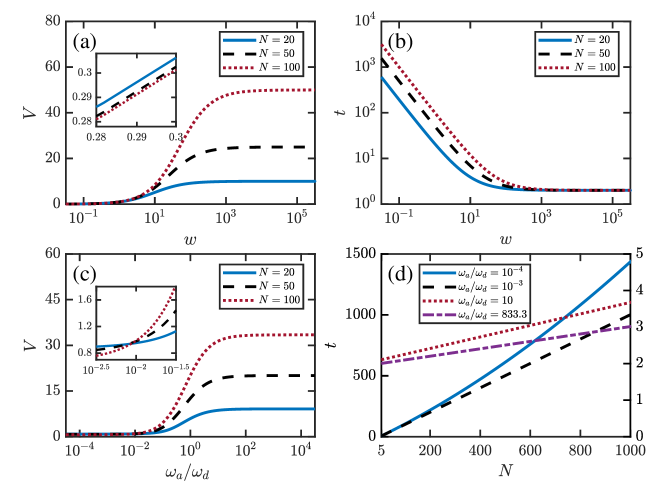
Figure 2: Dependence of (a) mean velocity $V$ and (b) mean dwell time $t$ on forward/backward diffusion rate $w$, where the fast binding rate $\omega_{a}=1000\times 10^{8}\text{ s}^{-1}$ and the unbinding rate $\omega_{d}=1.2\times 10^{8}\text{ s}^{-1}$, keeping their ratio $\omega_{d}/\omega_{a}=0.0012$ Hepp2016Kinetics . (c) Mean velocity $V$ as a function of binding/unbinding ratio $\omega_{a}/\omega_{d}$ with the inset displaying the detail in enlarged scale. (d) Mean dwell time $t$ of translocation as a function of the length of polymer chain with different ratio of the binding/unbinding rate. The solid line and the dashed line are plotted corresponding to the left axis, while the dotted line and dash dotted line are to the right axis. In (c) and (d), the diffusion rate is kept $w=10^{2}\text{ s}^{-1}$ and the unbinding rate $\omega_{d}$ is kept of order $10^{8}$. Thus, the binding/unbinding process is more than 2 orders of magnitude faster than the diffusion process. Other parameters used in calculations are $\omega_{s}=\omega_{e}=1\text{ s}^{-1}$.

Numerical results on mean translocation velocity $V$ are displayed in Fig. 2. When trailing binding sites (i.e., binding sites of a polymer chain lying in the target region) are occupied with chaperones in large probability, the polymer chain with a larger forward/backward diffusion rate will pass through the pore more rapidly, since its backward motion is hindered by chaperones. So translocation velocity increases with the diffusion rate $w$. This rise, however, will not last indefinitely, since for sufficiently large diffusion rate $w$, the translocation velocity will be limited by the binding/unbinding process of chaperones as well as the finite starting rate $\omega_{s}$ and ending rate $\omega_{e}$. See Fig. 2(a). With Eqs. (39, 19), it can be mathematically shown that

$$\lim_{w\rightarrow+\infty}V=\frac{N}{\widetilde{W}_{1}-q^{N-1}K}\,,\quad\textrm{with}\ \widetilde{W}_{1}=\frac{1}{\omega_{s}}+K\left(\frac{\omega_{a}}{\omega_{d}+\omega_{e}}+\frac{2-q}{1-q}\right)\,.$$

It means that there is an upper limit for mean velocity $V$ as diffusion rate $w$ tends to infinity. See Fig. 2(a) again. Besides, we notice that a longer polymer chain employs greater mean velocity provided high diffusion rate, since the restriction of finite starting rate $\omega_{s}$ and ending rate $\omega_{e}$ produces less impact on the overall mean velocity of a long polymer chain. On the contrary, if the diffusion rate $w$ is pretty low, it is the relatively rapid initiation and termination that guides the translocation. Then, shorter polymer chains gain higher mean velocity $V$ since that is when initiation along with termination carries more weights. See the inset of Fig. 2(a).

From another perspective, we consider the mean dwell time $t$ for some translocation, which can be calculated as

$$t=\frac{N}{V}=W_{1}+W_{2}\widetilde{S}^{2-N}+W_{3}(N-2)\,.$$ (46)

See Eqs. (39, 19) for the second equality. Here, the numerator $N$ is the length of a polymer chain and the denominator $V$ is the mean velocity of translocation. Eq. (46) shows that more time is required for the translocation of a longer polymer chain. According to the definition of constant $S$, if the diffusion rate $w$ is low, $S$ increases almost linearly with $w$, while $W_{1},W_{2},W_{3}$ are all insensitive to the low diffusion rate $w$. Therefore, Eq. (46) indicates that the relation between dwell time $t$ and diffusion rate $w$ follows power law approximately, when the polymer chain diffuses at a low diffusion rate $w$. See Fig. 2(b).

The dependence of mean velocity $V$ on the ratio of binding/unbinding rate of a chaperone is presented in Fig. 2(c). With high ratio $\omega_{a}/\omega_{d}$, the binding site lying in the target region will be more likely to be occupied with a chaperone, which will, then, help rectify the forward/backward diffusion. That is, high binding/unbinding ratio speeds up the translocation of a polymer chain. The dependence of mean velocity on ratio $\omega_{a}/\omega_{d}$ displays similar performance to that on diffusion rate $w$, as is shown in Fig. 2(a, c). If the ratio $\omega_{a}/\omega_{d}$ is large enough, mean translocation velocity $V$ increases with the length $N$ of a polymer chain and vice versa. See Fig. 2(c) and the inset. This is because the longer a polymer chain is, the less influence is likely to be exerted through the relatively low starting rate $\omega_{s}$ and ending rate $\omega_{e}$. Contrariwise, low ratio $\omega_{a}/\omega_{d}$ leads to the slow translocation of the main body part of a polymer chain, and the relatively large starting rate $\omega_{s}$ as well as ending rate $\omega_{e}$ plays a more active role in promoting the overall mean translocation velocity $V$ of a shorter polymer chain. It means that the mean velocity will decrease with the growth of the polymer length $N$.

Note that, experiments in Hepp2016Kinetics give a binding/unbinding ratio, which is approximate to $833.3$. Fig. 2(c) shows that the velocity $V$ is almost independent of ratio $\omega_{a}/\omega_{d}$ when $\omega_{a}/\omega_{d}\geq 833.3$, implying that the translocation process is limited by the forward/backward diffusion rate $w$ as well as starting rate $\omega_{s}$ and ending rate $\omega_{e}$. Moreover, the plots in Fig. 2(a, b) show that, for diffusion rate $w$ larger than $1000\text{ s}^{-1}$, mean velocity $V$ is also insensitive to the change of rate $w$. Therefore, the translocation of polymer chain is limited merely by the starting and the ending process when $\omega_{a}/\omega_{d}\geq 833.3$ and diffusion rate $w\geq 1000\text{ s}^{-1}$. Obviously, velocity $V$ increases with both rate $\omega_{s}$ and rate $\omega_{e}$, see Fig. 1(d) or Eqs. (39, 19). Note that, in Fig. 2(a, b), the ratio $\omega_{a}/\omega_{d}$ is always kept $833.3$.

The dependence of dwell time $t$ on length $N$ of a polymer chain, with different values of ratio $\omega_{a}/\omega_{d}$, is plotted in Fig. 2(d). One can easily find that $t$ increases almost linearly with $N$, especially for large binding/unbinding ratio $\omega_{a}/\omega_{d}$. It can been seen in Eq. (46) as well. Meanwhile, Fig. 2(d) also shows that dwell time $t$ decreases with the ratio $\omega_{a}/\omega_{d}$, since a polymer chain deserves high mean velocity $V$ provided with great binding/unbinding ratio $\omega_{a}/\omega_{d}$. See Fig. 2(c) and the definition of $t$ given in Eq. (46).

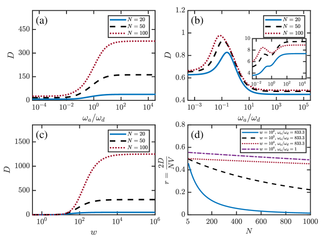
Figure 3: Effective diffusion constant $D$ as a function of the ratio $\omega_{a}/\omega_{d}$ is displayed in (a) and (b). The diffusion rate used in (a) is $w=10^{2}\text{ s}^{-1}$, while calculations in (b) are carried out with lower diffusion rates. $w=1\text{ s}^{-1}$ in (b) and $w=10\text{ s}^{-1}$ in inset. (c) Dependence of $D$ on the diffusion rate $w$, with ratio $\omega_{a}/\omega_{d}=833.3$ as is given in Hepp2016Kinetics . (d) The randomness, $r\equiv 2D/NV$, as a function of the length $N$ of a polymer chain. Several cases with different values of diffusion rate $w$ and ratio $\omega_{a}/\omega_{d}$ are considered. Detailed instructions on parameters are listed in the legend. Similar to Fig. 2, $\omega_{d}$ is held of order $10^{8}\text{ s}^{-1}$ to make the binding/unbinding process of a chaperone much faster than the forward/backward diffusion process of a polymer chain. Other parameters used in calculations are $\omega_{s}=1\text{ s}^{-1}$ and $\omega_{e}=1\text{ s}^{-1}$.

The discussion above on mean velocity $V$ provides a chief description of the dynamics of polymers’ translocation across membrane, but it is not sufficient for many biologically relevant cases, especially when the polymer chain is not long. In these situations, effective diffusion constant $D$, or say dispersion, plays an important role. The plots in Fig. 3(a) show that, for high diffusion rate $w$, diffusion constant $D$ increases with both the ratio $\omega_{a}/\omega_{d}$ and the polymer length $N$. At the same time, diffusion constant $D$ tends to its lower limit or upper limit monotonically as the ratio $\omega_{a}/\omega_{d}$ tends to 0 or infinity, respectively. However, something interesting happens as diffusion rate $w$ goes down approaching the starting rate $\omega_{s}$ and ending rate $\omega_{e}$. The plots in Fig. 3(b) show that, for such cases, $D$ will no longer change monotonically with rate $\omega_{a}/\omega_{d}$. Neither will it increase with the polymer length $N$. With a particular value of ratio $\omega_{a}/\omega_{d}=833.3$, as is given in Hepp2016Kinetics , the dependence of $D$ on diffusion rate $w$ is plotted in Fig. 3(c). As expected, $D$ increases with $w$ and tends to a limit rising with the polymer length $N$.

Compare Fig. 2(a, c) with Fig. 3(a, c), and one can find that mean velocity $V$ and effective diffusion constant $D$ show almost the same behavior. Both of them increase significantly when the parameter, either forward/backward diffusion rate $w$ or binding/unbinding ratio $\omega_{a}/\omega_{d}$, varies within some range. With the parameter varying beyond this range, however, mean velocity $V$ and effective diffusion constant $D$ both stay almost constant. The reason is that the dynamics of translocation process is regulated jointly by several factors. Besides diffusion rate $w$ along with the ratio $\omega_{a}/\omega_{d}$, these factors include starting rate $\omega_{s}$ and ending rate $\omega_{e}$. See Fig. 1. When the corresponding parameter, rate $w$ or $\omega_{a}/\omega_{d}$, varies within an appropriate range, the translocation process of a polymer is dominated by its diffusion process and the binding/unbinding process of a chaperone, and the mean velocity or diffusion constant changes significantly with the parameter, rate $w$ or ratio $\omega_{a}/\omega_{d}$. Otherwise, the dynamics of translocation will be limited by rate $\omega_{s}$ and $\omega_{e}$, and therefore is almost independent of the rate $w$ and ratio $\omega_{a}/\omega_{d}$. In other words, the translocation of a polymer chain across membrane consists of several kinetics, namely initiation, termination, binding/unbinding of chaperones and forward/backward diffusion of a polymer chain. For a given set of parameters, the overall translocation process may be limited by only one or some of them, with others fast enough to be neglected. But the limit process may be switched from one to another, with the change of one or some parameter values

It is also attractive to compare the degree of fluctuations of this stochastic process. An important dimensionless function to evaluate this quantity is randomness, which is defined as Kolomeisky2005Dynamic ; Svoboda1994Fluctuation

$$r=\frac{2D/N^{2}}{V/N}=\frac{2D}{NV}\,.$$

The plots in Fig. 3(d) show that, the randomness $r$ always decreases with the polymer length $N$. With the ratio $\omega_{a}/\omega_{d}=833.3$, which is consistent with Hepp2016Kinetics , $r$ increases with the forward/backward diffusion rate $w$. Our results also suggest a decrease of $r$ with the number of binding sites, i.e., $N$. A rapid decay in randomness $r$ can be observed on the condition of a low diffusion rate $w$, whereas the length of a polymer reduces $r$ slightly, but almost linearly, as long as the diffusion rate $w$ is high.

V Conclusions and Remarks

The “Brownian Ratchet” builds a general framework describing how diffusive motion is rectified by chemical energy. Particularly, the chaperone-assisted translocation of polymer chains across membrane constitutes a fine example of how directed motion can emerge from random diffusion, where the binding and unbinding of chaperones plays a prominent role.

In this paper, by mapping the process of translocation across membrane into the discrete motions of a membrane on the polymer chain, a theoretical model is presented, where the probability of finding membrane at some site of polymer chain is governed by usual master equations. With this model, the mean velocity and effective diffusion constant of translocation process can be derived explicitly, allowing us to discuss the dynamics of translocation across membrane much more efficiently.

Based on the exact expressions, detailed discussions on particular cases are presented, where the polymer chain is assumed to diffuse freely around the nanopore embedded in membrane if there is no chaperone molecule. Our results show that both the increase of forward/backward diffusion rate $w$ of polymer chain and the rise in binding/unbinding rate ratio $\omega_{a}/\omega_{d}$ of chaperones raise the mean translocation velocity monotonically to a polymer length dependent limit. With large diffusion rate $w$ or great ratio $\omega_{a}/\omega_{d}$, the mean velocity increases with the length of polymer chain, while opposite performance can be observed when $w$ or $\omega_{a}/\omega_{d}$ stays at a low level. The effective diffusion constant also increases with the diffusion rate $w$, but it will exhibit complicated properties when regarded as a function of ratio $\omega_{a}/\omega_{d}$. Meanwhile, the randomness decreases monotonically with the length of a polymer chain.

For most of biological processes in living cells, mean velocity together with effective diffusion constant is usually sufficient to describe the basic dynamic properties. Nevertheless, higher orders moments, or say higher cumulants, can be obtained as well, simply via the same methods in this paper. Meanwhile, all of the transition rates are assumed to be independent of the site of a polymer chain in our discussion. But in a promoted model with site-dependent transition rates, explicit expressions for mean velocity and effective diffusion constant can still be obtained sketching the key idea of this study.

Appendix A Derivation of Eq. (45)

Since the final expression for diffusion constant $D$ does not depend on the undetermined constant $T_{0}$, we let $T_{0}=0$, which indicates both $X_{k}$s and $\widetilde{X}_{k}$s equal to zero. At the same time, $Y_{k}$ follows Eq. (34) and $\widetilde{Y}_{k}$ follows Eq. (35).

In the stationary-state limit, Eq. (41), Eq. (42) and Eq. (43) turn to

$$\frac{1}{2}D_{1}=\omega_{f}Y_{1}+\omega_{f_{0}}\sum_{k=2}^{N-1}Y_{k}+\omega_{f_{1}}\sum_{k=2}^{N-1}\widetilde{Y}_{k}-\omega_{b}\sum_{k=2}^{N}Y_{k}\,,$$ (47)

$$\frac{1}{2}D_{2}=\frac{1}{2}\left[\omega_{s}b_{0}+\omega_{f}b_{1}+\omega_{f_{0}}\sum_{k=2}^{N-1}b_{k}+\omega_{f_{1}}\sum_{k=2}^{N-1}\widetilde{b}_{k}+\omega_{b}\sum_{k=2}^{N}b_{k}\right]\,,$$ (48)

and

$$-\frac{1}{2}D_{3}=-A\left[Y_{1}+\sum_{k=2}^{N}(Y_{k}+\widetilde{Y}_{k})\right]\,.$$ (49)

Take Eq. (33) into Eq. (47),

$$\begin{split}\frac{1}{2}D_{1}=&(\omega_{f}Y_{1}-\omega_{b}Y_{2})+\sum_{k=2}^{N-1}(SY_{k}-RY_{k+1})-\frac{\omega_{f_{1}}}{\omega_{d}+\omega_{f_{1}}}\sum_{k=2}^{N-1}\widetilde{a}_{k}-(1-q)\omega_{b}\frac{\omega_{f_{1}}}{\omega_{d}+\omega_{f_{1}}}\sum_{k=2}^{N-1}b_{k+1}\,,\\ =&-\frac{\omega_{f_{1}}}{\omega_{d}+\omega_{f_{1}}}\sum_{k=2}^{N-1}\widetilde{a}_{k}-(1-q)\omega_{b}\frac{\omega_{f_{1}}}{\omega_{d}+\omega_{f_{1}}}\sum_{k=2}^{N-1}b_{k+1}+\sum_{k=1}^{N-1}r_{k}\,.\end{split}$$ (50)

With Eq. (30), we have

$$\sum_{k=1}^{N-1}r_{k}=-\frac{\omega_{d}}{\omega_{d}+\omega_{f_{1}}}\sum_{k=2}^{N-1}\widetilde{a}_{k}-R\sum_{k=2}^{N-1}b_{k+1}-\omega_{b}b_{2}+\omega_{s}b_{0}\sum_{k=1}^{N-1}k-\sum_{k=1}^{N-1}\sum_{i=1}^{k}a_{i}-\sum_{k=2}^{N-2}\sum_{i=2}^{k}\widetilde{a}_{i}\,.$$ (51)

Note that the summation of the first term in Eq. (50) and that in Eq. (51) is

$$-\frac{\omega_{f_{1}}}{\omega_{d}+\omega_{f_{1}}}\sum_{k=2}^{N-1}\widetilde{a}_{k}-\frac{\omega_{d}}{\omega_{d}+\omega_{f_{1}}}\sum_{k=2}^{N-1}\widetilde{a}_{k}=-\sum_{i=2}^{N-1}\widetilde{a}_{i}\,,$$

and the summation of terms related to $b_{k}$ in these two equations is shown as

$$-(1-q)\omega_{b}\frac{\omega_{f_{1}}}{\omega_{d}+\omega_{f_{1}}}\sum_{k=2}^{N-1}b_{k+1}-R\sum_{k=2}^{N-1}b_{k+1}-\omega_{b}b_{2}+\omega_{s}b_{0}\sum_{k=1}^{N-1}k=-\omega_{b}\sum_{k=2}^{N}b_{k}+\frac{1}{2}N(N-1)\omega_{s}b_{0}\,.$$

Then

$$\frac{1}{2}D_{1}=-\sum_{k=1}^{N-1}s_{k}-\sum_{k=2}^{N-1}\widetilde{s}_{k}-\omega_{b}\sum_{k=2}^{N}b_{k}+\frac{1}{2}N(N-1)\omega_{s}b_{0}\,,$$ (52)

where

$$s_{k}=\sum_{i=1}^{k}a_{i}\,,\quad\widetilde{s}_{k}=\sum_{i=2}^{k}\widetilde{a}_{i}\,.$$

For Eq. (48),

$$\begin{split}\frac{1}{2}D_{2}=&\frac{1}{2}\left[\omega_{s}b_{0}+\omega_{f}b_{1}+\omega_{f_{0}}\sum_{k=2}^{N-1}b_{k}+\omega_{f_{1}}\sum_{k=2}^{N-1}\widetilde{b}_{k}-\omega_{b}\sum_{k=2}^{N}b_{k}+2\omega_{b}\sum_{k=2}^{N}b_{k}\right]\\ =&\omega_{b}\sum_{k=2}^{N}b_{k}+\frac{1}{2}V\,.\end{split}$$ (53)

With Eq. (39), the summation of Eq. (52), Eq. (53) and Eq. (49) can be written as

$$\begin{split}D=&\frac{1}{2}(D_{1}+D_{2}-D_{3})\\ =&-\sum_{k=1}^{N-1}s_{k}-\sum_{k=2}^{N-1}\widetilde{s}_{k}+N\frac{V}{2}-V\left[Y_{1}+\sum_{k=2}^{N}(Y_{k}+\widetilde{Y}_{k})\right]\,,\end{split}$$

which is exactly Eq. (45).

References

- (1) W. Neupert and M. Brunner. The protein import motor of mitochondria. Nat. Rev. Mol. Cell Bio., 3:555–565, 2002.
- (2) T. A. Rapoport. Protein translocation across the eukaryotic endoplasmic reticulum and bacterial plasma membranes. Nature, 450:663–669, 2007.
- (3) W. Neupert. A perspective on transport of proteins into mitochondria: a myriad of open questions. J. Mol. Bio., 427:1135–1158, 2015.
- (4) H. Santos-Rosa, H. Moreno, G. Simos, A. Segref, B. Fahrenkrog, N. Panté, and E. Hurt. Nuclear mRNA export requires complex formation between Mex67p and Mtr2p at the nuclear pores. Mol. Cell. Biol., 18:6826–6838, 1998.
- (5) G. Schatz and B. Dobberstein. Common principles of protein translocation across membranes. Science, 271:1519–1526, 1996.
- (6) B. Albert, A. Johnson, J. Lewis, M. Raff, K. Roberts, and P. Walter. Molecular Biology of the Cell, 5th Ed.
- (7) S. Liu, G. Chistol, C. L. Hetherington, S. Tafoya, K. Aathavan, J. Schnitzbauer, S. Grimes, P. J. Jardine, and C. Bustamante. A viral packaging motor varies its DNA rotation and step size to preserve subunit coordination as the capsid fills. Cell, 157:702–713, 2014.
- (8) H. Salman, D. Zbaida, Y. Rabin, D. Chatenay, and M. Elbaum. Kinetics and mechanism of DNA uptake into the cell nucleus. Proc. Natl. Acad. Sci. USA, 98:7247–7252, 2001.
- (9) J. F. Allemand and B. Maier. Bacterial translocation motors investigated by single molecule techniques. FEMS Microbiol. Rev., 33:593–610, 2009.
- (10) B. Burton and D. Dubnau. Membrane-associated DNA transport machines. Cold Spring Harb. Perspect. Biol., 2:a000406, 2010.
- (11) I. Chen, P. J. Christie, and D. Dubnau. The ins and outs of DNA transfer in bacteria. Science, 310:1456–1460, 2005.
- (12) I. Chen and D. Dubnau. DNA uptake during bacterial transformation. Nat. Rev. Microbiol., 2:241–249, 2004.
- (13) E. P. Holowka, V. Z. Sun, D. T. Kamei, and T. J. Deming. Polyarginine segments in block copolypeptides drive both vesicular assembly and intracellular delivery. Nat. Mat., 6:52–57, 2007.
- (14) S. W. P. Turner, M. Cabodi, and H. G. Craighead. Confinement-induced entropic recoil of single DNA molecules in a nanofluidic structure. Phy. Rev. Lett., 88:128103, 2002.
- (15) J. J. Kasianowicz, E. Brandin, D. Branton, and D. W. Deamer. Characterization of individual polynucleotide molecules using a membrane channel. Proc. Natl. Acad. Sci. USA, 93:13770–13773, 1996.
- (16) A. Meller, L. Nivon, E. Brandin, J. Golovchenko, and D. Branton. Rapid nanopore discrimination between single polynucleotide molecules. Proc. Natl. Acad. Sci. USA, 97:1079–1084, 2000.
- (17) W. Sung and P. J. Park. Polymer translocation through a pore in a membrane. Phy. Rev. Lett., 77:783–786, 1996.
- (18) A. Meller, L. Nivon, and D. Branton. Voltage-driven DNA translocations through a nanopore. Phy. Rev. Lett., 86:3435–3438, 2001.
- (19) A. Corsi, A. Milchev, V. G. Rostiashvili, and T. A. Vilgis. Field-driven translocation of regular block copolymers through a selective liquid-liquid interface. Macromolecules, 39:7115–7124, 2006.
- (20) S. M. Simon, C. S. Peskin, and G. F. Oster. What drives the translocation of proteins? Proc. Natl. Acad. Sci. USA, 89:3770–3774, 1992.
- (21) C. S. Peskin, G. M. Odell, and G. F. Oster. Cellular motions and thermal fluctuations: the brownian ratchet. Biophys. J., 65:316–324, 1993.
- (22) T. C. Elston. Models of post-translational protein translocation. Biophys. J., 79:2235–2251, 2000.
- (23) K. E. S. Matlack, W. Mothes, and T. A. Rapoport. Protein translocation: tunnel vision. Cell, 92:381–390, 1998.
- (24) K. E. S. Matlack, B. Misselwitz, K. Plath, and T. A. Rapoport. BiP acts as a molecular ratchet during posttranslational transport of prepro- factor across the ER membrane. Cell, 97:553–564, 1999.
- (25) C. Hepp and B. Maier. Kinetics of DNA uptake during transformation provide evidence for a translocation ratchet mechanism. Proc. Natl. Acad. Sci. USA, 113:12467–12472, 2016.
- (26) R. Zandi, D. Reguera, J. Rudnick, and W. M. Gelbart. What drives the translocation of stiff chains? Proc. Natl. Acad. Sci. USA, 100:8649–8653, 2003.
- (27) T. Ambjörnsson and R. Metzler. Chaperone-assisted translocation. Phys. Biol., 1:77–88, 2004.
- (28) T. Ambjörnsson, M. A. Lomholt, and R. Metzler. Directed motion emerging from two coupled random processes: translocation of a chain through a membrane nanopore driven by binding proteins. J. Phys.- Condens. Matter, 17:S3945–S3964, 2005.
- (29) M. R. D’Orsogna, T. Chou, and T. Antal. Exact steady-state velocity of ratchets driven by random sequential adsorption. J. Phys. A-Math. Theor., 40:5575–5584, 2007.
- (30) P. L. Krapivsky and K. Mallick. Fluctuations in polymer translocation. J. Stat. Mech.-Theory E., 2010:P07007, 2010.
- (31) R. H. Abdolvahab, R. Metzler, and M. R. Ejtehadi. First passage time distribution of chaperone driven polymer translocation through a nanopore: homopolymer and heteropolymer cases. J. Chem. Phys., 135:245102.
- (32) M. Uhl and U. Seifert. Force-dependent diffusion coefficient of molecular brownian ratchets. Phys. Rev. E, 98:022402, 2018.
- (33) B. Derrida. Velocity and diffusion constant of a periodic one-dimensional hopping model. J. Stat. Phys., 31:433–450, 1983.
- (34) U. Gerland, J. D. Moroz, and T. Hwa. Physical constraints and functional characteristics of transcription factor-DNA interaction. Proc. Natl. Acad. Sci. USA, 99:12015–12020, 2002.
- (35) A. B. Kolomeisky and H. Phillips. Dynamic properties of motor proteins with two subunits. J. Phys.-Condens. Matter, 17:S3887–S3899, 2005.
- (36) K. Svoboda, P. P. Mitra, and S. M. Block. Fluctuation analysis of motor protein movement and single enzyme kinetics. Proc. Natl. Acad. Sci. USA, 91:11782–11786, 1994.