Hidden symmetries of two-field cosmological models

Abstract

We determine the most general time-independent Noether symmetries of two-field cosmological models with rotationally-invariant scalar manifold metrics. In particular, we show that such models can have hidden symmetries, which arise if and only if the scalar manifold metric has Gaussian curvature $-3/8$, i.e. when the model is of elementary $\alpha$-attractor type with a fixed value of the parameter $\alpha$. In this case, we find explicitly all scalar potentials compatible with hidden Noether symmetries, thus classifying all models of this type. We also discuss some implications of the corresponding conserved quantity.

1 Introduction

Cosmological models with two real scalar fields produce natural generalizations of single scalar field cosmology, which may be favored in fundamental theories of gravity OOSV ; GK ; OPSV ; AP . Pairs of real scalar fields arise naturally in supergravity and string theory. Indeed, the generic supersymmetric compactification of such theories produces complex moduli, each of which can be viewed as a pair of real scalars.

Scalar multifield models were considered in cosmology from various points of view (see, for example, PT1 ; PT2 ; Welling ; m1 ; m2 ; m3 ; m4 ), including numerically Dias1 ; Dias2 ; Mulryne and to some extent phenomenologically c1 . However, current insight into their dynamics (which, as outlined in flows ; Roest1 ; Roest2 , is quite interesting from the perspective of the geometric theory of dynamical systems Palis ) is far more limited than for one-field models. In particular, numerous questions regarding the behavior of such models have not been studied systematically.

In this paper, we address one fundamental problem regarding such models, namely the question of symmetries and conserved quantities. A general two-field cosmological model based on a simply connected and spatially-flat FLRW space-time with scale factor $a(t)$ is parameterized by a scalar manifold $(\Sigma,\mathcal{G})$ (a complete and connected two-dimensional Riemannian manifold which plays the role of target space for the non-linear sigma model describing the two scalar fields $\varphi^{1},\varphi^{2}$) and a scalar potential $V$ (a smooth real-valued function defined on $\Sigma$, which describes the self-interacting potential of the scalars). Here $\Sigma$ is the internal manifold of the two scalar fields, which we allow to have non-trivial topology (such as non-contractible cycles) while $\mathcal{G}$ is the scalar manifold metric, whose components locally determine the kinetic terms of the two scalar fields. The scalar kinetic terms are specified globally by the pair $(\Sigma,\mathcal{G})$. Such models admit a description (known traditionally as the “minisuperspace formulation”) as a Lagrangian system for the three degrees of freedom $a$, $\varphi^{1}$, $\varphi^{2}$ subject to a constraint (namely the zero energy shell condition), which implements the Friedmann equation. The minisuperspace formulation allows one to study symmetries of such models using the Noether approach. We followed this method in reference ABL — where we restricted to scalar manifolds which are rotationally invariant and we considered only a special class of time-independent symmetries satisfying a certain separation of variables Ansatz. In the present paper, we still assume that the scalar manifold metric $\mathcal{G}$ is rotationally invariant, but study the problem without making any other assumptions. This allows us to give a complete description of all time-independent Noether symmetries for models with rotationally-invariant scalar manifold metric and to classify Noether-symmetric models of this type. In particular, we find many new Noether symmetries that were never considered before, the vast majority of which do not satisfy the separation of variables Ansatz used in reference ABL . Most of these symmetries, which we describe explicitly, are not invariant under the $\mathrm{U}(1)$ group of rotations which preserves the scalar manifold metric.

Using the minisuperspace description, we first show that any time-independent Noether symmetry of a general two-field cosmological model is a direct sum of a visible symmetry with a Hessian symmetry. The first of these are obvious symmetries, corresponding to those continuous isometries of the scalar manifold which preserve the scalar potential $V$; such symmetries do not involve the cosmological scale factor $a$. On the other hand, Hessian symmetries are hidden, in the sense that they are not immediately obvious; they involve $a$ as well as an auxiliary real-valued smooth function $\Lambda$ (called the generating function of the corresponding Hessian symmetry), which is defined on the scalar manifold $\Sigma$. For Hessian symmetries, the Noether condition dictates that $\Lambda$ must satisfy a system of two linear partial differential equations, namely the so-called Hesse equation (a second order PDE for $\Lambda$ which depends only on the scalar manifold metric) and the $\Lambda$-$V$ equation (a relation which involves the scalar manifold metric and the first order partial derivatives of $\Lambda$ and $V$). The Hesse equation relates the Hessian tensor of $\Lambda$ to the symmetric tensor $\Lambda\mathcal{G}$ and a solution of this equation will be called a Hesse function. The two-field cosmological model is called weakly Hessian if its scalar manifold admits non-trivial Hesse functions. The model is called Hessian if it admits a Hessian symmetry, i.e. if it is weakly Hessian and its scalar potential $V$ satisfies the $\Lambda$-$V$ equation for some non-trivial Hesse function $\Lambda$ of the scalar manifold. A Hessian model can also admit visible symmetries, provided that its scalar potential is sufficiently special. We show that the conservation law associated to a Hessian symmetry allows one to compute the e-fold number along cosmological trajectories without performing an integral, thereby providing a useful tool for extracting phenomenologically relevant information in Hessian two-field models.

When $\mathcal{G}$ is rotationally invariant, we show that the model is weakly Hessian iff $\Sigma$ is diffeomorphic to a disk, a punctured disk or an annulus and $\mathcal{G}$ is a metric of constant Gaussian curvature $K=-\frac{3}{8}$. In particular, weakly-Hessian two-field cosmological models coincide with those elementary two-field $\alpha$-attractor models (in the sense of reference elem ) for which $\alpha=\frac{8}{9}$ (here and in the following we use the convention $K=-\frac{1}{3\alpha}$), being special examples of the much wider class of two-field generalized $\alpha$-attractors introduced and studied in genalpha ; elem ; modular ; cosmunif . We show that such weakly-Hessian models are Hessian iff their scalar potential has a specific form which we determine explicitly in all cases, thereby classifying all Hessian two-field models with rotationally invariant scalar manifold metric. When the scalar manifold is a disk endowed with its complete metric of Gaussian curvature $-3/8$, we find that Hessian models fall naturally into three classes (which we call “timelike”, “spacelike” and “lightlike”), distinguished by the orbit type of their Hesse generating function under the natural action of the group of orientation-preserving isometries of the hyperbolic disk. In this case, the space of Hesse functions is three-dimensional and can be identified with the Minkowski space $\mathbb{R}^{1,2}$. Thus Hesse functions are naturally parameterized by a Minkowski 3-vector $B$, whose timelike, spacelike or lightlike character determines the type of the model. For each of the three types, we give the explicit general form of the scalar potential which is compatible with a Hessian symmetry, as well as the explicit form of the corresponding Hesse generator. When the scalar manifold is a punctured disk or an annulus endowed with a metric of Gaussian curvature $-3/8$, we find that the space of Hesse functions is one-dimensional and determine it, also giving the explicit form of the scalar potential for which the two-field model is Hessian. In each case mentioned above, we also describe the special situation when the Hessian model admits visible symmetries. These results allow for a complete description of time-independent Noether symmetries in two-field cosmological models with rotationally invariant scalar manifold metric. As we will show in a separate paper, a deeper mathematical approach allows one to prove that these are in fact the only Hessian models, hence the results derived herein provide a complete classification of Hessian cosmological two-field models.

The paper is organized as follows. Section 2 briefly recalls the minisuperspace description of two-field cosmological models. Section 3 gives a geometric characterization of time-independent Noether symmetries in such models, showing that any such symmetry can be written as a direct sum between a visible and a Hessian symmetry. In particular, we prove that the generating function $\Lambda$ of a Hessian symmetry satisfies the Hesse and $\Lambda$-$V$ equations, showing how the latter can be used to determine $V$ in terms of $\Lambda$ through the method of characteristics. We also discuss the integral of motion of a Hessian symmetry, showing that it can be used to extract an algebraic (as opposed to integral) formula in terms of the scalars $\varphi^{i}$ for the number of e-folds along cosmological trajectories. Section 4 gives the classification of weakly-Hessian models with rotationally-invariant scalar manifold metric, summarizing the results proved in Appendix C. This shows that the only scalar manifolds which are allowed in such models are the disk, punctured disk and annuli of constant Gaussian curvature $K=-\frac{3}{8}$. It follows that weakly-Hessian models with rotationally-invariant scalar manifold metric are elementary two-field $\alpha$-attractors in the sense of reference elem , for the specific value $\alpha=\frac{8}{9}$. We next proceed to determine the general form of the scalar potential of the corresponding Hessian models in each of the three cases. The hyperbolic disk is discussed in Section 5. In this case, the results of Appendix C imply that the space of Hesse functions is three dimensional and admits a basis formed by the classical Weierstrass coordinates. This allows us to identify the space of Hesse functions with the Minkowski 3-space $\mathbb{R}^{1,2}$, on which the group of orientation-preserving isometries of the hyperbolic disk acts through proper and orthochronous Lorentz transformations (as recalled in Appendix B). This provides a natural classification of Hesse functions into functions of timelike, spacelike and lightlike type. For each of these three cases, we use the method of characteristics for the $\Lambda$-$V$ equation and representation-theoretic arguments to extract the explicit general expression for those scalar potentials $V$ for which the model admits the Hessian symmetry generated by a given Hesse function $\Lambda$. We also describe the special cases when a Hessian model admits visible symmetries. In Section 6, we determine explicitly the scalar potential of Hessian two-field cosmological models whose scalar manifold is a punctured disk of Gaussian curvature $-\frac{3}{8}$ and explain when such models also admit visible symmetries. In Section 7, we perform the same analysis for models whose target is a hyperbolic annulus of Gaussian curvature $-\frac{3}{8}$. Finally, Section 8 gives our conclusions and some directions for further research. In the appendices, we review or derive various technical results used in the main text.

Notations and conventions.

Throughout this paper, all manifols considered are assumed to be connected, paracompact, Hausdorff and smooth. The scalar manifold of a two-field cosmological model is assumed to be complete, as required by conservation of energy; for simplicity, we also assume it to be oriented. By a hyperbolic metric we always mean a metric which is complete and of unit negative Gaussian curvature. The notation $\mathrm{D}$ indicates the Euclidean disk of unit radius, while $\dot{\mathrm{D}}\stackrel{{\scriptstyle{\rm def.}}}{{=}}\mathrm{D}\setminus\{0\}$ indicates the punctured Euclidean disk. Finally, $A(R)$ (where $R>1$) indicates the Euclidean annulus of inner radius $1/R$ and outer radius $R$. The notations $\mathbb{D}$ and $\mathbb{D}^{\ast}$ indicate the surfaces $\mathrm{D}$ and $\dot{\mathrm{D}}$ when endowed with their unique hyperbolic metric, while $\mathbb{A}(R)$ indicates the annulus $A(R)$, when the latter is endowed with its unique hyperbolic metric of modulus $\mu=2\log R$. The isometry group of an oriented Riemannian 2-manifold $(\Sigma,\mathcal{G})$ is denoted by $\mathrm{Iso}(\Sigma,\mathcal{G})$, while its subgroup of orientation-preserving isometries is denoted by $\mathrm{Iso}_{+}(\Sigma,\mathcal{G})$. We refer the reader to the Appendices and to references genalpha ; elem for a summary of some relevant information about elementary hyperbolic surfaces.

2 The minisuperspace Lagrangian of two-field cosmological models

In this section, we recall briefly the definition of two-field cosmological models and their constrained Lagrangian description in the minisuperspace approach.

2.1 Two-field cosmological models

We consider cosmological models with two real scalar fields whose underlying space-time is a simply-connected and spatially flat FLRW universe. Our models are parameterized by a connected, oriented and complete Riemannian $2$-manifold $(\Sigma,\mathcal{G})$ (called the scalar manifold), together with a scalar potential given by a smooth real-valued function $V$ defined on $\Sigma$. This data combines into a scalar triple $(\Sigma,\mathcal{G},V)$. The condition that $\Sigma$ be connected and oriented is purely technical and it could be relaxed. The condition that the metric $\mathcal{G}$ is complete insures conservation of energy in such models.

The models are obtained from the following action, which describes the coupling of Einstein gravity defined on $\mathbb{R}^{4}$ with the non-linear sigma model of target space $(\Sigma,\mathcal{G})$ and scalar potential $V$:

$$\mathcal{S}[g,\varphi]:=\mathcal{S}_{\Sigma,\mathcal{G},V}[g,\varphi]\!=\!\!\int_{\mathbb{R}^{4}}\!\!\mathrm{d}^{4}x\,\sqrt{|\det g|}\left[\frac{R(g)}{2}-\frac{1}{2}g^{\mu\nu}\mathcal{G}_{ij}\partial_{\mu}\varphi^{i}\partial_{\nu}\varphi^{j}-V(\varphi)\right].$$ (1)

Here $R(g)$ is the scalar curvature of the space-time metric $g$ (which has ‘mostly plus’ signature), while $\varphi$ is a smooth map from $\mathbb{R}^{4}$ to $\Sigma$, whose components in local coordinates on $\Sigma$ (denoted $\varphi^{i}$ with $i=1,2$) are the two real scalar fields of the model. The cosmological model defined by the scalar triple $(\Sigma,\mathcal{G},V)$ is obtained from (1) by fixing $g$ to be the background metric of a simply-connected FLRW universe with flat spatial section:

$$\mathrm{d}s_{g}^{2}:=-\mathrm{d}t^{2}+a^{2}(t)\mathrm{d}\vec{x}^{2}~{}~{}(\mathrm{where}~{}~{}x^{0}=t~{}~{},~{}~{}\vec{x}=(x^{1},x^{2},x^{3})~{}~{}\mathrm{and}~{}~{}a(t)>0~{}~{}\forall t)$$ (2)

and taking $\varphi$ to depend only on the cosmological time $t$:

$$\varphi=\varphi(t)~{}~{}.$$ (3)

Let $H\stackrel{{\scriptstyle{\rm def.}}}{{=}}\frac{\dot{a}}{a}$ denote the Hubble parameter, where $\dot{a}\stackrel{{\scriptstyle{\rm def.}}}{{=}}\frac{\mathrm{d}a}{\mathrm{d}t}$.

2.2 The minisuperspace Lagrangian

Substituting (2) and (3) in (1) and ignoring the integration over the spatial variables $\vec{x}$ gives the minisuperspace action:

$$S[a,\varphi]=\int_{-\infty}^{+\infty}\!\mathrm{d}t\,a^{3}\!\left[\frac{3(\dot{a}^{2}+a\ddot{a})}{a^{2}}+\frac{1}{2}\mathcal{G}_{ij}(\varphi)\dot{\varphi}^{i}\dot{\varphi}^{j}-V(\varphi)\right]~{},$$ (4)

where $\dot{\varphi}\stackrel{{\scriptstyle{\rm def.}}}{{=}}\frac{\mathrm{d}\varphi}{\mathrm{d}t}$. Notice that $S$ depends explicitly on the scale factor $a$ of the FLRW metric. The functional (4) can be viewed as the classical action of a mechanical system with three degrees of freedom. Indeed, integration by parts in the $\ddot{a}$ term of (4) allows us to write:

$$S[a,\varphi]=\int_{-\infty}^{\infty}\!\mathrm{d}t\,L(a(t),\dot{a}(t),\varphi(t),\dot{\varphi}(t))~{}~{},$$ (5)

where $L:=L_{(\Sigma,\mathcal{G},V)}$ is the minisuperspace Lagrangian:

$$L(a,\dot{a},\varphi,\dot{\varphi})\stackrel{{\scriptstyle{\rm def.}}}{{=}}-3a\dot{a}^{2}+a^{3}\left[\frac{1}{2}\mathcal{G}_{ij}(\varphi)\dot{\varphi}^{i}\dot{\varphi}^{j}-V(\varphi)\right]~{}.$$ (6)

In this formulation, the triplet $(a,\varphi^{i})$ provides local coordinates on the configuration space:

$$\mathcal{N}\stackrel{{\scriptstyle{\rm def.}}}{{=}}\mathbb{R}_{>0}\times\Sigma~{}~{}$$ (7)

of this mechanical system. The Euler-Lagrange equations of (6) take the form:

$$3H^{2}+2\dot{H}+\frac{1}{2}\mathcal{G}_{ij}(\varphi)\dot{\varphi}^{i}\dot{\varphi}^{j}-V(\varphi) = 0$$ (8)

$$(\nabla_{t}+3H)\dot{\varphi}^{j}+\mathcal{G}^{ij}(\varphi)(\partial_{i}V)(\varphi) = 0~{}~{}.$$

Here $\nabla_{t}\dot{\varphi}^{i}\stackrel{{\scriptstyle{\rm def.}}}{{=}}\ddot{\varphi}^{i}+\Gamma^{i}_{jk}\dot{\varphi}^{j}\dot{\varphi}^{k}$, where $\Gamma^{i}_{jk}$ are the Christoffel symbols of the scalar manifold metric $\mathcal{G}$, $\partial_{i}V\stackrel{{\scriptstyle{\rm def.}}}{{=}}\frac{\partial V}{\partial\varphi^{i}}$ and we used the relation:

$$\frac{2a\ddot{a}+\dot{a}^{2}}{a^{2}}=3H^{2}+2\dot{H}~{}~{}.$$

To recover the cosmological equations of motion, one must subject the Lagrangian (6) to the zero energy constraint $E_{L}=\frac{\partial L}{\partial\dot{a}}\dot{a}+\frac{\partial L}{\partial\dot{\varphi}^{i}}\dot{\varphi}^{i}-L=0$, which takes the following explicit form:

$$\frac{1}{2}\mathcal{G}_{ij}(\varphi)\dot{\varphi}^{i}\dot{\varphi}^{j}+V(\varphi)=3H^{2}~{}~{},$$ (9)

thus coinciding with the time-time component of the equations of motion derived from (1). This is often called the Friedmann constraint. On solutions of the Euler-Lagrange equations (8), this constraint gives a relation between the integration constants, thus reducing the number of independent constants by one (see, for instance, reference CR ). However, one can also use the Friedmann constraint from the outset to solve algebraically for the Hubble parameter $H$:

$$H=\frac{1}{\sqrt{6}}\left[\mathcal{G}_{ij}(\varphi)\dot{\varphi}^{i}\dot{\varphi}^{j}+2V(\varphi)\right]^{1/2}~{}.$$ (10)

To recapitulate, the system formed by the Euler-Lagrange equations (8) together with the Friedmann constraint (9) is equivalent with the cosmological equations of the two-field model obtained from (1).

3 Noether symmetries for general two-field models

In this section, we consider time-independent infinitesimal Noether symmetries of the minisuperspace Lagrangian (6). By analyzing the Noether symmetry condition, we show that the corresponding Noether generator decomposes as a direct sum between a visible and a hidden symmetry, the latter type of symmetry being determined by a Hesse function $\Lambda$. For Hessian symmetries, we explain how the $\Lambda$-$V$ equation allows one to extract the general form of the scalar potential using the method of characteristics. We also discuss the natural action of the isometry group of the scalar manifold on the linear space of all Hesse functions and on the linear space of all scalar potentials which satisfy the $\Lambda$-$V$ equation. Finally, we consider the conservation law associated to a Hessian symmetry, showing that it allows one to determine the number of e-folds along cosmological trajectories algebraically in $\varphi^{i}$, instead of through an integral.

3.1 Noether generators and integrals of motion

Recall that the configuration space $\mathcal{N}=\mathbb{R}_{>0}\times\Sigma$ of the minisuperspace model is a product of the target space $\Sigma$ (which is locally parameterized by $\varphi^{1}$ and $\varphi^{2}$) with the range $\mathbb{R}_{>0}$ of the scale factor $a$. Geometrically, the Lagrangian (6) is a smooth real-valued function defined on the tangent bundle $T\mathcal{N}$, which identifies naturally with the first jet bundle of curves of $\mathcal{N}$ (see Olver ). This tangent bundle decomposes as:

$$T\mathcal{N}=T_{(a)}\mathcal{N}\oplus T_{(\varphi)}\mathcal{N}~{}~{},$$

where $T_{(a)}\mathcal{N}$ is the pullback of the tangent bundle of the half-line $\mathbb{R}_{>0}$ through the first projection and $T_{(\varphi)}\mathcal{N}$ is the pullback of the tangent bundle of $\Sigma$ through the second projection. Hence any vector field $X$ defined on $\mathcal{N}$ decomposes uniquely as:

$$X=X_{(a)}+X_{(\varphi)}~{}~{},$$

where $X_{(a)}$ is a vector field defined on the half-line and $X_{(\varphi)}$ is a vector field defined on $\Sigma$. In local coordinates on the configuration space $\mathcal{N}$, we have:

$$X_{(a)}=X^{a}(a,\varphi)\frac{\partial}{\partial a}~{}~{},~{}~{}X_{(\varphi)}=X^{i}(a,\varphi)\frac{\partial}{\partial\varphi^{i}}~{}~{}.$$ (11)

The first jet prolongation $\mathcal{X}$ of $X$ is a vector field defined on $T\mathcal{N}$ which is given in local coordinates by the formula (see Olver ):

$$\mathcal{X}=X+\dot{X}^{a}(a,\varphi,\dot{a},\dot{\varphi})\frac{\partial}{\partial\dot{a}}+\dot{X}^{i}(a,\varphi,\dot{a},\dot{\varphi})\frac{\partial}{\partial\dot{\varphi}^{i}}~{}~{},$$

where:

$$\dot{\lambda}(a,\varphi,\dot{a},\dot{\varphi})\stackrel{{\scriptstyle{\rm def.}}}{{=}}(\partial_{t}\lambda)(a,\varphi)+(\partial_{a}\lambda)(a,\varphi)\dot{a}+(\partial_{i}\lambda)(a,\varphi)\dot{\varphi}^{i}$$

for any smooth function $\lambda$, where we use the notations $\partial_{t}\stackrel{{\scriptstyle{\rm def.}}}{{=}}\frac{\partial}{\partial t}$, $\partial_{a}\stackrel{{\scriptstyle{\rm def.}}}{{=}}\frac{\partial}{\partial a}$, $\partial_{i}\stackrel{{\scriptstyle{\rm def.}}}{{=}}\frac{\partial}{\partial\varphi^{i}}$ . The vector field $X$ is a variational symmetry of the Lagrangian (6) provided that it satisfies the Noether condition:

$$\mathcal{L}_{\mathcal{X}}(L)=0~{}~{},$$ (12)

where $\mathcal{L}_{\mathcal{X}}$ denotes the Lie derivative with respect to the prolongation $\mathcal{X}$. In local coordinates on $\Sigma$, this condition takes the form:

$$P(a,\varphi,\dot{a},\dot{\varphi})=0~{}~{},$$ (13)

where the polynomial $P$ is given by:

$$P(a,\varphi,\dot{a},\dot{\varphi})\stackrel{{\scriptstyle{\rm def.}}}{{=}}X^{a}\frac{\partial L}{\partial a}+X^{i}\frac{\partial L}{\partial\varphi^{i}}+\dot{X}^{a}\frac{\partial L}{\partial\dot{a}}+\dot{X}^{i}\frac{\partial L}{\partial\dot{\varphi}^{i}}~{}~{}.$$ (14)

Given a variational symmetry $X$ of $L$, the associated integral of motion has the following local expression (see Olver ):

$$\mathrm{J}_{X}=X^{a}\partial_{\dot{a}}L+X^{i}\partial_{\dot{\varphi}^{i}}L=-6a\dot{a}X^{a}+\mathcal{G}_{ij}(\varphi)a^{3}X^{i}\dot{\varphi}^{j}~{}~{}.$$ (15)

3.2 The characteristic system

In this subsection, we show that the Noether symmetry condition (12) for the minisuperspace Lagrangian (6) amounts to the requirement that $X$ has the form $X(a,\varphi)=X_{(a)}(a,\varphi)+X_{(\varphi)}(a,\varphi)=X^{a}\partial_{a}+X^{i}\partial_{i}$, with:

$$X_{(a)}(a,\varphi)=\frac{\Lambda(\varphi)}{\sqrt{a}}\partial_{a}~{}~{},~{}~{}X_{(\varphi)}(a,\varphi)=\left[Y^{i}(\varphi)-\frac{4}{a^{3/2}}\mathcal{G}^{ij}(\varphi)\partial_{j}\Lambda(\varphi)\right]\!\partial_{i}~{}~{},$$ (16)

where $\Lambda$ is a smooth real-valued function defined on $\Sigma$ and $Y=Y^{i}\partial_{i}$ is a smooth vector field defined on $\Sigma$, which satisfy the characteristic system:

$$\left(\partial_{i}\partial_{j}-\Gamma_{ij}^{k}\partial_{k}\right)\Lambda=\frac{3}{8}\mathcal{G}_{ij}\Lambda$$

$$\mathcal{G}^{ij}\partial_{i}V\partial_{j}\Lambda=\frac{3}{4}V\Lambda$$

$$\nabla_{i}Y_{j}+\nabla_{j}Y_{i}=0~{}~{}$$

$$Y^{i}\partial_{i}V=0~{}~{}~{}.$$

In index-free notation, the general Noether generator reads:

$$X=X_{\Lambda}+Y~{}~{},$$ (18)

where:

$$X_{\Lambda}=\frac{\Lambda}{\sqrt{a}}\partial_{a}-\frac{4}{a^{3/2}}\mathrm{grad}_{\mathcal{G}}\Lambda~{}~{}.$$ (19)

Let us begin by computing the polynomial (14):

$$P = 3a^{2}X^{a}\left[-H^{2}+\frac{1}{2}\mathcal{G}_{ij}\dot{\varphi}^{i}\dot{\varphi}^{j}-V\right]+a^{3}X^{i}\left[\frac{1}{2}\partial_{i}\mathcal{G}_{jk}\dot{\varphi}^{j}\dot{\varphi}^{k}-\partial_{i}V\right]$$

$$-6a^{2}H\dot{X}^{a}+a^{3}\mathcal{G}_{ij}\dot{\varphi}^{j}\dot{X}^{i}~{}~{}.$$

Using $H=\frac{\dot{a}}{a}$ and expanding in powers of $\dot{a}$ and $\dot{\varphi}$ gives:

$$P=P_{o}(a,\varphi)+P_{00}(a,\varphi)\dot{a}^{2}+P_{0i}(a,\varphi)\dot{a}\dot{\varphi}^{i}+P_{ij}(a,\varphi)\dot{\varphi}^{i}\dot{\varphi}^{j}~{}~{},$$

where:

$$P_{00} = -3X^{a}-6a\partial_{a}X^{a}$$

$$P_{0i} = -6a\partial_{i}X^{a}+a^{3}\mathcal{G}_{ij}\partial_{a}X^{j}$$

$$P_{ij}=P_{ji} = \frac{3}{2}a^{2}\mathcal{G}_{ij}X^{a}+a^{3}\frac{1}{2}\left(\nabla_{i}X_{j}+\nabla_{j}X_{i}\right)~{}~{}$$ (20)

$$P_{o} = -3a^{2}VX^{a}-a^{3}X^{i}\partial_{i}V~{}~{}.$$

Explicitly, the $a^{3}$-term of $P_{ij}$ reads:

$$\frac{1}{2}\left(\nabla_{i}X_{j}+\nabla_{j}X_{i}\right)=\frac{1}{2}\left(\partial_{i}X_{j}+\partial_{j}X_{i}-2\Gamma_{ij}^{k}X_{k}\right)$$

$$=\frac{1}{2}\left[(\partial_{k}\mathcal{G}_{ij})X^{k}+\mathcal{G}_{ki}\partial_{j}X^{k}+\mathcal{G}_{kj}\partial_{i}X^{k}\right]~{}~{}.$$

Using (3.2), the Noether symmetry condition (13) amounts to the system:

$$(\mathrm{coeff.~{}of}~{}\dot{a}^{2}~{})~{}~{}~{}:~{}~{}X^{a}+2a\partial_{a}X^{a}=0$$

$$(\mathrm{coeff.~{}of}~{}\dot{a}\dot{\varphi}^{i})~{}~{}:~{}-6\partial_{i}X^{a}+a^{2}\mathcal{G}_{ij}\partial_{a}X^{j}=0$$

$$(\mathrm{coeff.~{}of}~{}\dot{\varphi}^{i}\dot{\varphi}^{j})~{}:~{}3\mathcal{G}_{ij}X^{a}+a\left(\nabla_{i}X_{j}+\nabla_{j}X_{i}\right)=0~{}~{}$$ (21)

$$(\mathrm{potential~{}term})~{}:~{}3VX^{a}+aX^{i}\partial_{i}V=0~{}~{}.$$

The first equation in (3.2) implies that the first relation in (16) holds for some smooth function $\Lambda(\varphi)$. Using this into the second equation of (3.2) gives:

$$\mathcal{G}_{ij}\partial_{a}X^{j}=6\frac{\partial_{i}\Lambda}{a^{5/2}}~{}~{}.$$ (22)

Integrating (22) with respect to $a$ gives the second relation in (16):

$$X^{i}(a,\varphi)=-\frac{4}{a^{3/2}}\mathcal{G}^{ij}\partial_{j}\Lambda(\varphi)+Y^{i}(\varphi)~{}~{},$$ (23)

where $Y$ is a vector field defined on $\Sigma$. Substituting (16) into the third equation of (3.2) gives:

$$\frac{1}{a^{1/2}}\left[3\mathcal{G}_{ij}\Lambda-4(\nabla_{i}\partial_{j}\Lambda+\nabla_{j}\partial_{i}\Lambda)\right]+a(\nabla_{i}Y_{j}+\nabla_{j}Y_{i})=0~{}~{}.$$ (24)

Since the terms multiplying powers of $a$ in this relation are themselves independent of $a$, taking the limits $a\rightarrow 0$ and $a\rightarrow\infty$ shows that (24) is equivalent with the first and third equations of the characteristic system (3.2). Finally, substituting (16) into the fourth equation of (3.2) gives:

$$\frac{1}{a^{1/2}}\left[3V\Lambda-4\mathcal{G}^{ij}\partial_{j}\Lambda\partial_{i}V\right]+aY^{i}\partial_{i}V=0~{}~{}.$$ (25)

Again taking the limits $a\rightarrow 0$ and $a\rightarrow\infty$ shows that (25) is equivalent with the second and fourth equations of (3.2). This completes the proof that the characteristic system (3.2) is equivalent with the Noether symmetry condition (12).

The integral of motion (15) of the Noether symmetry (16) described by a solution $(\Lambda,Y)$ of the characteristic system takes the form:

$$\mathrm{J}_{X}=-6a\dot{a}X^{a}+\mathcal{G}_{ij}(\varphi)a^{3}X^{i}\dot{\varphi}^{j}=-6\dot{a}\sqrt{a}\Lambda(\varphi)+a^{3}\mathcal{G}_{ij}(\varphi)Y^{i}(\varphi)\dot{\varphi}^{j}-4a^{3/2}\dot{\Lambda}~{}~{},$$

i.e.:

$$\mathrm{J}_{X}=-4\frac{\mathrm{d}}{\mathrm{d}t}\left[a^{3/2}\Lambda(\varphi)\right]+a^{3}\mathcal{G}_{ij}(\varphi)Y^{i}(\varphi)\dot{\varphi}^{j}~{}~{}.$$ (26)

3.3 Natural subsystems of the characteristic system. Hessian and visible symmetries

Notice that those equations of the system (3.2) which contain $\Lambda$ decouple from those equations which contain $Y$. Hence the characteristic system naturally splits into two subsystems of partial differential equations, namely:

the $\Lambda$-system:

$$\nabla_{i}\partial_{j}\Lambda=\frac{3}{8}\mathcal{G}_{ij}\Lambda$$

$$\mathcal{G}^{ij}\partial_{i}V\partial_{j}\Lambda=\frac{3}{4}V\Lambda~{}~{}$$ (27)

and the $Y$-system:

$$\nabla_{i}Y_{j}+\nabla_{j}Y_{i}=0$$

$$Y^{i}\partial_{i}V=0~{}~{}.$$ (28)

A vector field of the form (16) for which $Y=0$ and $\Lambda$ is a smooth solution of the $\Lambda$-system will be called an infinitesimal Hessian symmetry of $(\Sigma,\mathcal{G},V)$. A scalar triple which admits Hessian symmetries will be called a Hessian triple; in this case, the corresponding two-field cosmological model will be called a Hessian model. On the other hand, a vector field of the form (16) for which $\Lambda=0$ and the vector field $Y$ is a non-trivial smooth solution of the $Y$-system will be called an infinitesimal visible symmetry of $(\Sigma,\mathcal{G},V)$. A scalar triple which admits visible symmetries is called a visibly symmetric triple and the corresponding two-field cosmological model will be called a visibly-symmetric model.

The result proved in the previous subsection implies that any time-independent infinitesimal Noether symmetry of the minisuperspace system decomposes as a direct sum of a visible symmetry with a Hessian symmetry. Notice that infinitesimal visible symmetries coincide with those Killing vector fields of $(\Sigma,\mathcal{G})$ which generate isometries preserving the scalar potential $V$; they are the ‘obvious’ symmetries of the two-field cosmological model defined by the scalar triple $(\Sigma,\mathcal{G},V)$. Unlike visible symmetries, Hessian symmetries are not geometrically obvious and can be viewed as ‘hidden symmetries’ of the model. Also notice that the first and third equations in (3.2) do not depend on $V$. For a given scalar manifold $(\Sigma,\mathcal{G})$, these equations can be solved for $\Lambda$ and $Y$. Fixing solutions $(\Lambda,Y)$ of these two equations, the second and fourth equations of the characteristic system can then be used to determine the scalar potential in terms of $\Lambda$ and $Y$.

3.4 Rescaling the scalar manifold metric. The Hesse and $\Lambda$-$V$ equations

It is convenient to consider the rescaled scalar manifold metric:

$$G\stackrel{{\scriptstyle{\rm def.}}}{{=}}\beta^{2}\mathcal{G}=\frac{3}{8}\mathcal{G}\Longleftrightarrow\mathcal{G}=\frac{1}{\beta^{2}}G=\frac{8}{3}G~{}~{},$$ (29)

where:

$$\beta\stackrel{{\scriptstyle{\rm def.}}}{{=}}\sqrt{\frac{3}{8}}~{}~{}.$$ (30)

Since the Levi-Civita connection of $\mathcal{G}$ is invariant under such a rescaling, the $\Lambda$-system becomes:

$$\nabla\mathrm{d}\Lambda=G\Lambda$$

$$\langle\mathrm{d}V,\mathrm{d}\Lambda\rangle_{G}=2V\Lambda~{}~{},$$ (31)

while the $Y$-system preserves its form when expressed with respect to the rescaled metric $G$.

The first equation in (3.4):

$$\nabla\mathrm{d}\Lambda=G\Lambda~{}~{},$$ (32)

(whose left hand side equals the Hessian tensor of $\Lambda$ computed with respect to the scalar manifold metric $\mathcal{G}$) will be called the Hesse equation of the rescaled scalar manifold $(\Sigma,G)$ and its smooth solutions $\Lambda$ will be called Hesse functions of $(\Sigma,G)$. Let $\mathcal{S}(\Sigma,G)$ denote the linear space of such functions. A Riemannian manifold $(\Sigma,G)$ is called Hesse if it admits non-trivial Hesse functions, i.e. if $\mathcal{S}(\Sigma,G)\neq 0$. The second equation in (3.4):

$$\langle\mathrm{d}V,\mathrm{d}\Lambda\rangle_{G}=2V\Lambda$$ (33)

will be called the $\Lambda$-$V$ equation of the rescaled scalar triple $(\Sigma,G,V)$. Let $\mathcal{V}(G,\Lambda)$ denote the linear space of smooth functions $V$ satisfying this equation.

The Hesse equation (32) is invariant under the natural action:

$$\Lambda\rightarrow\Lambda\circ\psi^{-1}~{}~{},~{}~{}\forall\psi\in\mathrm{Iso}(\Sigma,G)$$

of the isometry group $\mathrm{Iso}(\Sigma,G)=\mathrm{Iso}(\Sigma,\mathcal{G})$ of the scalar manifold. In particular, such transformations preserve the space $\mathcal{S}(\Sigma,G)$ of Hesse functions of $(\Sigma,G)$. Similarly, equation (33) is invariant under the natural action of the isometry group of the scalar manifold on the pair $(V,\Lambda)$:

$$(\Lambda,V)\rightarrow(\Lambda\circ\psi^{-1},V\circ\psi^{-1})~{}~{},~{}\forall\psi\in\mathrm{Iso}(\Sigma,G)~{}~{}.$$

Hence an isometry of $(\Sigma,G)$ takes the general solution of (33) into the general solution of the same equation, but with $\Lambda$ replaced by $\Lambda\circ\psi^{-1}$:

$$\mathcal{V}(G,\Lambda\circ\psi^{-1})=\mathcal{V}(G,\Lambda)\circ\psi^{-1}~{}~{},~{}~{}\forall\psi\in\mathrm{Iso}(\Sigma,G)~{}~{},~{}~{}\forall\Lambda\in\mathcal{S}(\Sigma,G)~{}~{}.$$ (34)

Remark 3.1.

Equation (33) is invariant under rescalings $\Lambda\rightarrow C\Lambda$, where $C$ is any non-zero constant. This implies that the general solution of this equation is unchanged if one rescales $\Lambda$ by $C$:

$$\mathcal{V}(G,C\Lambda)=\mathcal{V}(G,\Lambda)~{}~{},~{}~{}\forall C\in\mathbb{R}\setminus\{0\}~{}~{}.$$

In particular, the general solution of the $\Lambda$-$V$ equation (33) depends only on the ray of $\Lambda$ in the real projective space $\mathbb{P}\mathcal{S}(\Sigma,G)$.

3.5 The scalar potential of a Hessian symmetry

Given a Hesse function $\Lambda\in\mathcal{S}(\Sigma,G)$, consider the $\Lambda$-$V$-equation (33) with $G=\beta^{2}\mathcal{G}$ as defined in (29):

$$\langle\mathrm{d}V,\mathrm{d}\Lambda\rangle_{\mathcal{G}}=2\beta^{2}V\Lambda~{}~{},$$ (35)

where $\langle\mathrm{d}V,\mathrm{d}\Lambda\rangle_{\mathcal{G}}=\langle\mathrm{grad}_{\mathcal{G}}V,\mathrm{grad}_{\mathcal{G}}\Lambda\rangle_{\mathcal{G}}=\mathcal{G}^{ij}\partial_{i}V\partial_{j}\Lambda$.

One can solve (35) through the method of characteristics (see Appendix A). For this, let $\gamma$ be a $\mathcal{G}$-gradient flow curve of $\Lambda$ with gradient flow parameter $q$:

$$\frac{\mathrm{d}\gamma(q)}{\mathrm{d}q}=-(\mathrm{grad}_{\mathcal{G}}\Lambda)(\gamma(q))~{}~{}.$$ (36)

Then (36) and (35) imply:

$$\frac{\mathrm{d}}{\mathrm{d}q}V(\gamma(q))=-\langle\mathrm{grad}_{\mathcal{G}}V,\mathrm{grad}_{\mathcal{G}}\Lambda\rangle_{\mathcal{G}}\Big{|}_{\gamma(q)}=-\langle\mathrm{d}V,\mathrm{d}\Lambda\rangle_{\mathcal{G}}\Big{|}_{\gamma(q)}=-2\beta^{2}\Lambda(\gamma(q))V(\gamma(q))~{}~{},$$

which gives:

$$V(\gamma(q))=V(\gamma(q_{0}))\,e^{\stackrel{{\scriptstyle-2\beta^{2}\!\!\bigintssss_{q_{0}}^{q}{\Lambda\mathrm{d}q}}}{{\!\!\!\!\!\!\!\gamma}}}~{}~{}.$$ (37)

It is convenient to use the restriction $\lambda=\Lambda\circ\gamma$ (i.e. $\lambda(q)=\Lambda(\gamma(q))$) of $\Lambda$ to $\gamma$ as a parameter on the gradient flow curve (notice that $\lambda$ decreases with $q$). We have:

$$\frac{\mathrm{d}\lambda}{\mathrm{d}q}=(\mathrm{d}_{\gamma(q)}\Lambda)\left(\frac{\mathrm{d}\gamma(q)}{\mathrm{d}q}\right)=-||(\mathrm{grad}_{\mathcal{G}}\Lambda)(\gamma(q))||^{2}_{\mathcal{G}}=-||(\mathrm{d}\Lambda)(\gamma(q))||^{2}_{\mathcal{G}}~{}~{},$$

which gives:

$$\mathrm{d}q=-\frac{\mathrm{d}\lambda}{||\mathrm{d}\Lambda||^{2}_{\mathcal{G}}}~{}~{}.$$ (38)

Hence (37) becomes:

$$V(\gamma(q))=V(\gamma(q_{0}))\,e^{\stackrel{{\scriptstyle 2\beta^{2}\bigintssss_{\Lambda(\gamma(q_{0}))}^{\Lambda(\gamma(q))}{\frac{\lambda\mathrm{d}\lambda}{||\mathrm{d}\Lambda||_{\mathcal{G}}^{2}}}}}{{\!\!\!\!\!\!\!\!\!\!\!\!\!\!\!\!\!\!\!\!\!\!\!\!\!\!\!\!\!\!\gamma}}}~{}~{}.$$ (39)

This relation allows us to find the general solution of (35), provided that we can determine the gradient flow of $\Lambda$. To deal with the initial conditions, one can choose a section of the gradient flow, i.e. a (possibly disconnected) submanifold $\mathcal{Q}:=\mathcal{Q}_{\Lambda}$ of $\Sigma$ with the property that each gradient flow curve $\gamma$ of $\Lambda$ meets $\mathcal{Q}$ in exactly one point. For any $p\in\Sigma$, let $\gamma$ be the gradient flow curve which passes through $p$ and meets $\mathcal{Q}$ at the point $p_{0}$ (namely, we have $\gamma(q)=p$ and $\gamma(q_{0})=p_{0}$. Then relation (39) gives:

$$V(p)=V(p_{0})\,e^{\stackrel{{\scriptstyle 2\beta^{2}\bigintssss_{\Lambda(p_{0})}^{\Lambda(p)}{\frac{\lambda\mathrm{d}\lambda}{||\mathrm{d}\Lambda||_{\mathcal{G}}^{2}}}}}{{\!\!\!\!\!\!\!\!\!\!\!\!\!\!\!\!\!\!\!\!\!\!\gamma}}}~{}~{}.$$

The correspondence $p\rightarrow p_{0}$ defines a smooth function $F=F_{\mathcal{Q}}:\mathcal{Q}\rightarrow\Sigma$ which allows us to write the previous equation as:

$$V(p)=\omega(p)\,e^{\stackrel{{\scriptstyle 2\beta^{2}\bigintssss_{\Lambda(F(p))}^{\Lambda(p)}{\frac{\lambda\mathrm{d}\lambda}{||\mathrm{d}\Lambda||_{\mathcal{G}}^{2}}}}}{{\!\!\!\!\!\!\!\!\!\!\!\!\!\!\!\!\!\!\!\!\!\!\!\!\!\!\!\!\gamma}}}~{}~{},$$ (40)

where $\omega\stackrel{{\scriptstyle{\rm def.}}}{{=}}V\circ F$ is a real-valued smooth function defined on $\mathcal{Q}$.

Remark 3.2.

Given any non-zero constant $C$, the gradient flow of $\Lambda$ coincides with that of $C\Lambda$, up to a constant rescaling $q\rightarrow q/C$ of the gradient flow parameter.

3.6 The integral of motion of a Hessian symmetry

For a Hessian symmetry ($Y=0$) with generator $\Lambda$, the integral of motion (26) gives:

$$a(t)^{3/2}\Lambda(\varphi(t))=C-\frac{\mathrm{J}_{\Lambda}}{4}(t-t_{0})~{}~{},~{}~{}\mathrm{where}~{}~{}C=a_{0}^{3/2}\Lambda_{0}~{}~{}$$ (41)

and we defined:

$$a_{0}\stackrel{{\scriptstyle{\rm def.}}}{{=}}a(t_{0})~{}~{},~{}~{}\Lambda_{0}\stackrel{{\scriptstyle{\rm def.}}}{{=}}\Lambda(\varphi(t_{0}))~{}~{}.$$

The conserved quantity $\mathrm{J}_{\Lambda}$ is independent of $t$ along every solution of the Euler-Lagrange equations (but depends on the initial conditions of the solution). Differentiating (41) with respect to time at $t=t_{0}$ gives:

$$\!\!\!-\frac{\mathrm{J}_{\Lambda}}{4}\!=\!\frac{\mathrm{d}}{\mathrm{d}t}\left[a(t)^{3/2}\Lambda(\varphi(t))\right]\!\Big{|}_{t=t_{0}}\!\!\!\!=a_{0}^{3/2}\!\left[\frac{3}{2}H_{0}\Lambda_{0}\!+\!(\mathrm{d}_{\varphi(t_{0})}\Lambda)(\dot{\varphi}_{0})\right],$$ (42)

where $H_{0}\stackrel{{\scriptstyle{\rm def.}}}{{=}}H(t_{0})$ is determined by the Friedmann constraint (assuming that $H(t)>0$):

$$H_{0}=\frac{1}{\sqrt{6}}\left[||\dot{\varphi}_{0}||_{\mathcal{G}}^{2}+2V(\varphi_{0})\right]^{1/2}~{}~{}.$$

Here:

$$\varphi_{0}\stackrel{{\scriptstyle{\rm def.}}}{{=}}\varphi(t_{0})~{}~{}\mathrm{and}~{}~{}\dot{\varphi}_{0}\stackrel{{\scriptstyle{\rm def.}}}{{=}}\dot{\varphi}(t_{0})~{}~{}.$$

Relation (42) allows one to determine $\mathrm{J}_{\Lambda}$ from the initial conditions of the cosmological trajectory, while (41) determines the $t$-dependence of the cosmological scale factor along the trajectory:

$$a(t)=\left[\frac{C-\frac{\mathrm{J}_{\Lambda}}{4}(t-t_{0})}{\Lambda(\varphi(t))}\right]^{2/3}=a_{0}\left[\frac{\Lambda_{0}+\left(\frac{3}{2}H_{0}\Lambda_{0}+(\mathrm{d}_{\varphi_{0}}\Lambda)(\dot{\varphi}_{0})\right)(t-t_{0})}{\Lambda(\varphi(t))}\right]^{2/3}.$$ (43)

In turn, this determines the e-fold function $N_{t_{0}}(t)=\log\left[\frac{a(t)}{a(t_{0})}\right]$ along any given scalar field trajectory $\varphi(t)$, where $t_{0}$ is a reference cosmological time:

$$N_{t_{0}}(t)=\frac{2}{3}\log\left[\frac{\Lambda_{0}+\left(\frac{3}{2}H_{0}\Lambda_{0}+(\mathrm{d}_{\varphi_{0}}\Lambda)(\dot{\varphi}_{0})\right)(t-t_{0})}{\Lambda(\varphi(t))}\right]~{}~{}.$$ (44)

In particular, a scalar field trajectory which is inflationary for the cosmological time interval $[t_{0},t]$ will produce a desired number $N$ of e-folds during that time interval provided that its initial and final points $\varphi(t_{0}),\varphi(t)\in\Sigma$ satisfy the condition:

$$e^{\frac{3N}{2}}\Lambda(\varphi(t))-\Lambda_{0}=\left(\frac{3}{2}H_{0}\Lambda_{0}+(\mathrm{d}_{\varphi_{0}}\Lambda)(\dot{\varphi}_{0})\right)(t-t_{0})~{}~{}.$$ (45)

Remark 3.3.

The e-fold function is also determined as follows by the Friedmann constraint:

$$N_{t_{0}}(t)=\int_{t_{0}}^{t}H(\tau)\mathrm{d}\tau=\frac{1}{\sqrt{6}}\int_{t_{0}}^{t}\Big{[}||\dot{\varphi}(\tau)||_{\mathcal{G}}^{2}+2V(\varphi(\tau))\Big{]}^{1/2}\mathrm{d}\tau~{}~{}.$$ (46)

This non-local relation involves integration of a complicated quantity depending on both $\varphi(\tau)$ and $\dot{\varphi}(\tau)$ for $\tau\in[0,t]$, unlike the much simpler formula (44) (which involves no integrations).

Differentiating (44) with respect to $t$ gives:

$$H(t)=\frac{2}{3}\frac{\frac{3}{2}H_{0}\Lambda_{0}\!+\!(\mathrm{d}_{\varphi_{0}}\Lambda)(\dot{\varphi}_{0})}{\Lambda_{0}\!+\!\Big{(}\!\frac{3}{2}H_{0}\Lambda_{0}\!+\!(\mathrm{d}_{\varphi_{0}}\Lambda)(\dot{\varphi}_{0})\!\Big{)}(t\!-\!t_{0})}\!-\!\frac{(\mathrm{d}_{\varphi(t)}\Lambda)(\dot{\varphi}(t))}{\Lambda(\varphi(t))}~{}~{}.$$ (47)

The case $\dot{\varphi}_{0}=0$.

When $\dot{\varphi}_{0}=0$, relation (45) reduces to:

$$\left[1+\frac{3H_{0}}{2}(t-t_{0})\right]\frac{\Lambda_{0}}{\Lambda_{\varphi}(t)}=e^{\frac{3}{2}N_{t_{0}}(t)}~{}~{},$$ (48)

where $H_{0}=\frac{1}{\sqrt{3}}V_{0}^{1/2}>0$ with $V_{0}\stackrel{{\scriptstyle{\rm def.}}}{{=}}V(\varphi_{0})$ and we defined $\Lambda_{\varphi}(t)\stackrel{{\scriptstyle{\rm def.}}}{{=}}\Lambda(\varphi(t))$. On the other hand, relation (47) reduces to the following condition when $\dot{\varphi}_{0}=0$:

$$H(t)=\frac{2H_{0}}{2+3H_{0}(t-t_{0})}-\frac{\dot{\Lambda}_{\varphi}(t)}{\Lambda_{\varphi}(t)}~{}~{}.$$ (49)

Hence positivity of $H$ requires:

$$\frac{\dot{\Lambda}_{\varphi}}{\Lambda_{\varphi}}<\frac{2H_{0}}{2+3H_{0}(t-t_{0})}~{}~{}\mathrm{i.e.}~{}~{}\frac{\Lambda_{\varphi}(t)}{\Lambda_{0}}<\left[2+3H_{0}(t-t_{0})\right]^{2/3}~{}~{}.$$ (50)

Let:

$$s(t)\stackrel{{\scriptstyle{\rm def.}}}{{=}}3H_{0}-[2+3(t-t_{0})H_{0}]\frac{\dot{\Lambda}_{\varphi}(t)}{\Lambda_{\varphi}}~{}~{}.$$ (51)

Then condition (50) amounts to:

$$s(t)>H_{0}~{}~{}.$$ (52)

Recall that the inflationary time periods of the cosmological trajectory are defined by the condition that $a$ is a convex and strictly increasing function of $t$, i.e. $\dot{a}(t)>0$ and $\ddot{a}(t)>0$. Using (48), this amounts to requiring that the function:

$$a(t)=a(t_{0})\left(\left[1+\frac{3}{2}H_{0}(t-t_{0})\right]\frac{\Lambda_{0}}{\Lambda_{\varphi}(t)}\right)^{2/3}$$ (53)

be convex and strictly increasing. Let us assume that $\Lambda(t)>0$ along the trajectory (hence $\Lambda_{0}>0$). Since (52) implies $\dot{a}(t)>0$, the requirement for inflation amounts to $\ddot{a}(t)>0$, i.e.:

$$\frac{\ddot{\Lambda}_{\varphi}(t)}{\Lambda_{\varphi}(t)}<\frac{s(t)[5s(t)-18H_{0}]}{3[2+3H_{0}(t-t_{0})]^{2}}~{}~{}.$$ (54)

Conditions (52) and (54) can be used to determine the upper limit $t_{f}$ of an inflationary time interval $[t_{0},t_{f}]$ for which $\dot{\varphi}_{0}=0$.

4 Weakly-Hessian models with rotationally-invariant scalar manifolds

In this section, we give the characteristic system for models with rotationally-invariant scalar manifold metrics and the classification of weakly-Hessian two-field models. The proof of this classification is given in Appendix C. As shown in that appendix, the scalar manifold of any weakly-Hessian model is a disk, a punctured disk or an annulus, endowed with its complete metric of Gaussian curvature $K=-3/8$. We also list the general solutions of the Hesse equation in each of the three cases, solutions which are derived in the same appendix. In the next sections, we will consider each case in turn, extracting the explicit form of the scalar potential for which the corresponding weakly-Hessian models admit a Hessian symmetry.

4.1 The characteristic system

Consider the case when $\Sigma$ is diffeomorphic with the unit disk $\mathrm{D}$ or with the punctured unit disk $\dot{\mathrm{D}}$, endowed with a metric $\mathcal{G}$ which is rotationally-invariant:

$$\mathrm{d}s_{\mathcal{G}}^{2}=\mathrm{d}r^{2}+f(r)\mathrm{d}\theta^{2}~{}~{}.$$ (55)

Here $r$ and $\theta$ are normal polar coordinates for $\mathcal{G}$ and $f$ is a smooth and everywhere-positive real-valued function (which extends to the origin in the case $\Sigma\simeq\mathrm{D}$). For application to cosmological models, we must require that the scalar metric $\mathcal{G}$ is complete (otherwise the dynamics of the cosmological model would violate conservation of energy). The non-vanishing Christoffel symbols are:

$$\Gamma_{\theta\theta}^{r}=-\frac{f^{\prime}}{2}~{}~{},~{}~{}\Gamma^{\theta}_{r\theta}=\Gamma^{\theta}_{\theta r}=\frac{f^{\prime}}{2f}~{}~{},$$

while the Gaussian curvature of $\mathcal{G}$ takes the form:

$$K_{\mathcal{G}}=-\frac{(\sqrt{f})^{{}^{\prime\prime}}}{\sqrt{f}}=\frac{(f^{\prime})^{2}-2ff^{\prime\prime}}{4f^{2}}=-\frac{1}{2}\left(\frac{f^{\prime}}{f}\right)^{\prime}-\frac{1}{4}\left(\frac{f^{\prime}}{f}\right)^{2}~{}~{},$$ (56)

where we use the notation ${}^{\prime}=\frac{\mathrm{d}}{\mathrm{d}r}$. For such models, the Noether generator (16) takes the form:

$$X=\frac{\Lambda}{\sqrt{a}}\partial_{a}+\left[Y^{r}-\frac{4}{a^{3/2}}\partial_{r}\Lambda\right]\partial_{r}+\left[Y^{\theta}-\frac{4}{a^{3/2}f(r)}\partial_{\theta}\Lambda\right]\partial_{\theta}$$ (57)

Note that one can have both purely visible symmetries, i.e. with $\Lambda=0$ and $Y\neq 0$, and purely hidden symmetries, i.e. with $\Lambda\neq 0$ and $Y=0$. Let us write down the $Y$- and $\Lambda$-systems for the case of a rotationally-invariant metric $\mathcal{G}$.

The $Y$-system.

The $Y$-system (3.3) takes the form:

$$\partial_{r}Y^{r}=0$$

$$\partial_{\theta}Y^{r}+f\partial_{r}Y^{\theta}=0$$

$$\partial_{\theta}Y^{\theta}+\frac{f^{\prime}}{2f}Y^{r}=0$$ (58)

$$Y^{r}\partial_{r}V+Y^{\theta}\partial_{\theta}V=0~{}~{},$$

where the first three equations form the condition that $Y$ be a Killing vector.

Let $\mathcal{K}(\Sigma,\mathcal{G})$ denote the $\mathbb{R}$-vector space consisting of all Killing vector fields of $(\Sigma,\mathcal{G})$. Since the metric $\mathcal{G}$ is rotationally-invariant, the Killing equation has the obvious solution:

$$Y=\partial_{\theta}$$

and hence $\mathcal{K}(\Sigma,\mathcal{G})$ contains the one-dimensional subspace $\mathbb{R}\partial_{\theta}$. For a generic rotationally invariant metric, we have $\mathcal{K}(\Sigma,\mathcal{G})=\mathbb{R}\partial_{\theta}$, though in some cases the space of Killing vectors may be higher-dimensional. In the generic case, the last equation in (4.1) amounts to the condition that $V$ is $\mathrm{SO}(2)$-invariant, i.e.:

$$V=V(r)~{}~{}(\mathrm{indep.~{}of~{}}\theta)~{}~{}.$$

The $\Lambda$-system.

The $\Lambda$-system (3.3) takes the form:

$$\partial_{r}^{2}\Lambda=\frac{3}{8}\Lambda$$

$$\partial_{r}\partial_{\theta}\Lambda-\frac{f^{\prime}}{2f}\partial_{\theta}\Lambda=0$$

$$\partial_{\theta}^{2}\Lambda+\frac{f^{\prime}}{2}\partial_{r}\Lambda=\frac{3}{8}f\Lambda~{}~{}$$ (59)

$$\partial_{r}V\partial_{r}\Lambda+\frac{1}{f}\partial_{\theta}V\partial_{\theta}\Lambda=\frac{3}{4}V\Lambda~{}~{},$$

where the first three equations are equivalent with the Hesse condition (32).

Remark 4.1.

In reference ABL , we studied two-field rotationally invariant models with the separation of variables Ansatze: $X^{a}\!=\!A_{1}(a)R_{1}(r)\Theta_{1}(\theta)$ and $X^{i}\!=\!A^{i}(a)R^{i}(r)\Theta^{i}(\theta)$, assuming that each of the functions $A_{1}$, $R_{1}$, $\Theta_{1}$, $A^{i}$, $R^{i}$ and $\Theta^{i}$ is non-constant. Comparing with (16), one finds that these assumptions imply $Y=0$ as well as:

$$A_{1}=\frac{1}{\sqrt{a}}~{}~{},~{}~{}A^{i}=-\frac{1}{a^{3/2}}~{}~{},~{}~{}R_{1}(r)\Theta_{1}(\theta)=\Lambda~{}~{},~{}~{}R^{i}(r)\Theta^{i}(\theta)=4\mathcal{G}^{ij}\partial_{j}\Lambda~{}~{},$$ (60)

in agreement with ABL . Substituting $\Lambda=R_{1}(r)\Theta_{1}(\theta)$ in the first equation of (4.1) gives:

$$R_{1}(r)=C_{1}\cosh(\beta r)+C_{2}\sinh(\beta r)\quad,\quad\beta^{2}=\frac{3}{8}~{}~{},$$ (61)

which agrees with (ABL, , eq. (3.19)). Similarly, the second equation of (4.1) gives $\partial_{r}R_{1}=\frac{f^{\prime}}{2f}R_{1}$, where we used the assumption that $\Theta_{1}$ is not constant. Substituting $\partial_{r}R_{1}=\frac{f^{\prime}}{2f}R_{1}$ into the third equation of (4.1) gives:

$$8f\,\Theta_{1}^{\prime\prime}(\theta)+(2f^{\prime 2}-3f^{2})\,\Theta_{1}(\theta)=0\,\,\,,$$ (62)

which coincides with (ABL, , eq. (3.37)).

4.2 Classification of weakly-Hessian models with rotationally-invariant scalar manifold metric

The system formed by the first three equations in (4.1) is studied in detail in Appendix C; here we summarize the results of that analysis. As before, let $\beta\stackrel{{\scriptstyle{\rm def.}}}{{=}}\sqrt{\frac{3}{8}}$. For a rotationally-invariant Riemannian 2-manifold $(\Sigma,\mathcal{G})$, it is shown in Appendix C that the first three equations of the system (4.1) admit solutions iff the metric $\mathcal{G}$ has Gaussian curvature equal to $-\beta^{2}$, i.e. iff the rescaled metric $G=\beta^{2}\mathcal{G}$ has Gaussian curvature $-1$. In particular, the rescaled scalar manifold $(\Sigma,G)$ is a Hesse manifold in the sense of Subsection 3.4 iff it is a hyperbolic surface. Since $(\Sigma,G)$ is rotationally-invariant, a well-known result (which is summarized in Appendix D) implies that $(\Sigma,G)$ must be elementary hyperbolic, i.e. that it is isometric with the Poincaré disk $\mathbb{D}$, with the hyperbolic punctured disk $\mathbb{D}^{\ast}$ or with a hyperbolic annulus $\mathbb{A}(R)$ of modulus $\mu=2\log R$ (where $R>1$). We refer the reader to Appendix D and to reference elem for the description of elementary hyperbolic surfaces. We will use the notations $\mathbb{D}_{\beta}$, $\mathbb{D}^{\ast}_{\beta}$ and $\mathbb{A}_{\beta}(R)$ for the disk, punctured disk and annulus endowed with the metric $\mathcal{G}=\frac{1}{\beta^{2}}G$ of Gaussian curvature equal to $-\beta^{2}$. Then the following statements hold (see Appendix C):

1. If $(\Sigma,\mathcal{G})=\mathbb{D}_{\beta}$, then we have:

   $$f(r)=\frac{1}{\beta^{2}}\sinh^{2}(\beta r)~{}~{}$$ (63)

   and:

   $$\mathrm{d}s^{2}_{\mathcal{G}}=\mathrm{d}r^{2}+\frac{1}{\beta^{2}}\sinh^{2}(\beta r)\,\mathrm{d}\theta^{2}~{},$$ (64)

   with $r\geq 0$. In this case, the general solution of the Hesse equation of $(\Sigma,G)$ is given by:

   $$\Lambda(r,\theta)=B_{0}\cosh(\beta r)+\sigma\sinh(\beta r)\cos(\theta-\theta_{0})~{}~{},$$ (65)

   where $B_{0}$ (denoted ${\hat{B}}_{1}$ in Appendix C) and $\theta_{0}$ are arbitrary real constants, while $\sigma\geq 0$ is a non-negative constant (denoted $\frac{\zeta}{\beta}$ in Appendix C).

   In particular, the space of Hesse functions on the hyperbolic disk is three-dimensional. Let $(\rho,\theta)$ be Euclidean polar coordinates on the disk, related to the normal polar coordinates $(r,\theta)$ of the metric $\mathcal{G}$ through (cf. (207)):

   $$\rho\!=\!\tanh(\beta r/2)\in[0,1)\Longleftrightarrow r\!=\!\frac{2}{\beta}\operatorname{arctanh}(\rho)\!=\!\frac{1}{\beta}\log\frac{1\!+\!\rho}{1\!-\!\rho}\in[0,+\infty)~{}.$$ (66)

   Then (64) becomes:

   $$\mathrm{d}s^{2}_{\mathcal{G}}=\frac{4}{\beta^{2}(1-\rho^{2})^{2}}(\mathrm{d}\rho^{2}+\rho^{2}\mathrm{d}\theta^{2})=\frac{4}{\beta^{2}(1-\rho^{2})^{2}}(\mathrm{d}x^{2}+\mathrm{d}y^{2})~{}~{},$$ (67)

   where $x=\rho\cos\theta$ and $y=\rho\sin\theta$, while (65) takes the form:

   $$\Lambda(\rho,\theta)=\frac{B_{0}(1+\rho^{2})+2\sigma\rho\cos(\theta-\theta_{0})}{1-\rho^{2}}~{}~{}.$$ (68)

   Notice the relations:

   $$\beta r=2\operatorname{arctanh}(\rho)=\log\frac{1+\rho}{1-\rho}~{}~{}\mathrm{i.e.}~{}~{}\rho=\tanh\left(\frac{\beta r}{2}\right)=\frac{e^{\beta r}-1}{e^{\beta r}+1}~{}~{},$$ (69)

   the second of which implies:

   $$\cosh(\beta r)=\frac{1+\rho^{2}}{1-\rho^{2}}~{}~{},~{}~{}\sinh(\beta r)=\frac{2\rho}{1-\rho^{2}}~{}~{}.$$ (70)

2. If $(\Sigma,\mathcal{G})=\mathbb{D}^{\ast}_{\beta}$, then we have:

   $$f(r)=\frac{1}{(2\pi\beta)^{2}}e^{-2\beta r}~{}~{}$$ (71)

   and:

   $$\mathrm{d}s^{2}_{\mathcal{G}}=\mathrm{d}r^{2}+\frac{1}{(2\pi\beta)^{2}}e^{-2\beta r}\mathrm{d}\theta^{2}~{}~{},$$ (72)

   with $r\in\mathbb{R}$. In this case, the general solution of the Hesse equation (32) is given by:

   $$\Lambda(r)=Ce^{-\beta r}~{},$$ (73)

   where $C$ (denoted ${\hat{B}}$ in Appendix C) is an arbitrary constant. In particular, the space of Hesse functions on the hyperbolic punctured disk is one-dimensional. Let $(\rho,\theta)$ be Euclidean polar coordinates on the punctured disk, related to the normal polar coordinates $(r,\theta)$ of the metric $\mathcal{G}$ through (cf. eqs. (214)):

   $$\rho=e^{-2\pi e^{\beta r}}\in(0,1)\Longleftrightarrow r=\frac{1}{\beta}\log\left(\frac{|\log\rho|}{2\pi}\right)\in(-\infty,\infty)~{}~{}.$$ (74)

   Then (72) becomes:

   $$\mathrm{d}s^{2}_{\mathcal{G}}=\frac{1}{\beta^{2}(\rho\log\rho)^{2}}(\mathrm{d}\rho^{2}+\rho^{2}\mathrm{d}\theta^{2})=\frac{1}{\beta^{2}(\rho\log\rho)^{2}}(\mathrm{d}x^{2}+\mathrm{d}y^{2})~{}~{},$$ (75)

   while (73) takes the form:

   $$\Lambda(\rho)=\frac{2\pi C}{|\log\rho|}~{}~{}.$$ (76)

3. If $(\Sigma,\mathcal{G})=\mathbb{A}_{\beta}(R)$, then we have:

   $$f(r)=\frac{\ell^{2}}{(2\pi\beta)^{2}}\cosh^{2}(\beta r)~{}~{}$$ (77)

   and:

   $$\mathrm{d}s^{2}_{\mathcal{G}}=\mathrm{d}r^{2}+\frac{\ell^{2}}{(2\pi\beta)^{2}}\cosh^{2}(\beta r)\,\mathrm{d}\theta^{2}~{}~{},$$ (78)

   where $r\in\mathbb{R}$ and $\ell>0$ is given in (10). In this case, the general solution of the Hesse equation is:

   $$\Lambda(r)=C\sinh(\beta r)~{}~{},$$ (79)

   where $C$ (denoted ${\hat{B}}_{2}$ in Appendix C) is an arbitrary constant. In particular, the space of Hesse functions on any hyperbolic annulus is one-dimensional. Let $(\rho,\theta)$ be Euclidean polar coordinates on the annulus, related to the normal polar coordinates $(r,\theta)$ of the metric $\mathcal{G}$ through (cf. eqs. (219)):

   $$\rho=e^{-\frac{\mu}{\pi}\arccos\left[\frac{1}{\cosh(\beta r)}\right]}\Longleftrightarrow|r|=\frac{1}{\beta}\operatorname{arccosh}\left[\frac{1}{\cos\left(\frac{\pi}{\mu}|\log\rho|\right)}\right]~{}~{}.$$ (80)

   Then (78) becomes:

   $$\mathrm{d}s^{2}_{\mathcal{G}}\!=\!\left(\frac{\pi}{2\beta\log R}\right)^{2}\!\frac{\mathrm{d}\rho^{2}\!+\!\rho^{2}\mathrm{d}\theta^{2}}{\left[\rho\cos\left(\frac{\pi\log\rho}{2\log R}\right)\right]^{2}}\!=\!\left(\frac{\pi}{2\beta\log R}\right)^{2}\!\frac{\mathrm{d}x^{2}+\mathrm{d}y^{2}}{\left[\rho\cos\left(\frac{\pi\log\rho}{2\log R}\right)\right]^{2}}~{},$$ (81)

   while (79) takes the following form:

   $$\Lambda(\rho)=C\tan\left(\frac{\pi}{\mu}\log\rho\right)~{}~{}.$$ (82)

5 Hessian models for the hyperbolic disk

In this section, we show that the space $\mathcal{S}(\mathbb{D})$ of Hesse functions on the hyperbolic disk identifies naturally with the 3-dimensional Minkowski space $\mathbb{R}^{1,2}$ such that the natural action of the orientation-preserving isometry group of $\mathbb{D}$ on such functions identifies with the fundamental action of the group of proper and orthochronous Lorentz transformations in 3 dimensions. The identification follows from the fact that the general Hesse function on the hyperbolic disk is a linear combination of the components of the classical Weierstrass map and hence the classical Weierstrass coordinates of $\mathbb{D}$ form a basis for the space of Hesse functions. This leads to a description of Hesse functions on the hyperbolic disk in terms of three-dimensional Minkowski geometry and allows for a natural classification of such functions into functions of timelike, spacelike and lightlike type. We also discuss the level sets and critical points of such functions, showing that they behave quite differently in each of the three cases. For each type, we show that the gradient flow of a Hesse function can be described explicitly in certain classical coordinate systems on the hyperbolic disk. Finally, we combine these results and the method of characteristics to extract the explicit form of the most general scalar potential which solves the $\Lambda$-$V$ equation, thus classifying all Hessian two-field cosmological models whose rescaled scalar manifold is a hyperbolic disk. We find that such scalar potentials admit a natural description in terms of three-dimensional Minkowski geometry. The results of this section are summarized in Subsection 5.6, which the reader may consult first. Throughout this section, $G$ denotes the Poincaré metric (which has Gaussian curvature equal to $-1$), while $\mathcal{G}$ denotes the physically-relevant metric (which has Gaussian curvature equal to $-\beta^{2}=-3/8$).

5.1 The space of Hesse functions

We start by studying the space of Hesse functions on the hyperbolic disk $\mathbb{D}=(\mathrm{D},G)$.

The Weierstrass basis.

The general Hesse function (65) of $\mathbb{D}$ can be written as:

$$\Lambda\!=\!B_{0}\cosh(\beta r)\!+\!B_{1}\sinh(\beta r)\cos\theta\!+\!B_{2}\sinh(\beta r)\sin\theta=\!\frac{B_{0}(1\!+\!\rho^{2})\!+\!2B_{1}x\!+\!2B_{2}y}{1-\rho^{2}}~{},$$ (83)

where (see equation (209)):

$$B_{1}\stackrel{{\scriptstyle{\rm def.}}}{{=}}\sigma\cos\theta_{0}~{}~{},~{}~{}B_{2}\stackrel{{\scriptstyle{\rm def.}}}{{=}}\sigma\sin\theta_{0}~{}~{}.$$ (84)

Here $x=\rho\cos\theta$ and $y=\rho\sin\theta$ are Euclidean Cartesian coordinates on the disk (with $\rho=\sqrt{x^{2}+y^{2}}$) while $(r,\theta)$ are normal polar coordinates for the physically-relevant metric $\mathcal{G}=\frac{1}{\beta^{2}}G$; for the relation between $\rho$ and $r$, see (207). Relation (83) shows that the functions:

$$\Xi^{0}\!\stackrel{{\scriptstyle{\rm def.}}}{{=}}\!\frac{1+\rho^{2}}{1-\rho^{2}}\!=\!\cosh\beta r~{},~{}~{}\Xi^{1}\!\stackrel{{\scriptstyle{\rm def.}}}{{=}}\!\frac{2x}{1-\rho^{2}}\!=\!\sinh(\beta r)\cos\theta~{},~{}~{}\Xi^{2}\!\stackrel{{\scriptstyle{\rm def.}}}{{=}}\!\frac{2y}{1-\rho^{2}}\!=\!\sinh(\beta r)\sin\theta$$ (85)

form a basis of the linear space $\mathcal{S}(\mathbb{D})$ of smooth solutions to the Hesse equation. The fundamental solutions (85) coincide with the classical “Weierstrass coordinates” of $\mathbb{D}$, i.e. with the components of the Weierstrass map $\Xi:\mathrm{D}\rightarrow\mathbb{R}^{3}$ (see Appendix B) which realizes the hyperbolic disk as the future sheet:

$$S^{+}\stackrel{{\scriptstyle{\rm def.}}}{{=}}\big{\{}X=(X^{0},X^{1},X^{2})\,|\,X^{0}=\sqrt{1+(X^{1})^{2}+(X^{2})^{2}}\,\big{\}}$$

of the unit hyperboloid in the 3-dimensional Minkowski space $\mathbb{R}^{1,2}=(\mathbb{R},(~{},~{}))$ (see Figure 1). Here:

$$(X,X^{\prime})\stackrel{{\scriptstyle{\rm def.}}}{{=}}X^{0}{X^{\prime}}^{0}-X^{1}{X^{\prime}}^{1}-X^{2}{X^{\prime}}^{2}~{}~{}~{}~{}\forall X,X^{\prime}\in\mathbb{R}^{3}$$ (86)

is the Minkowski pairing of signature $(1,2)$, whose coefficients we denote by $\eta_{\mu\nu}$:

$$(\eta_{\mu\nu})_{\mu,\nu=0,\ldots 2}=\mathrm{diag}(1,-1,-1)~{}~{}$$

and which we use to raise and lower indices.

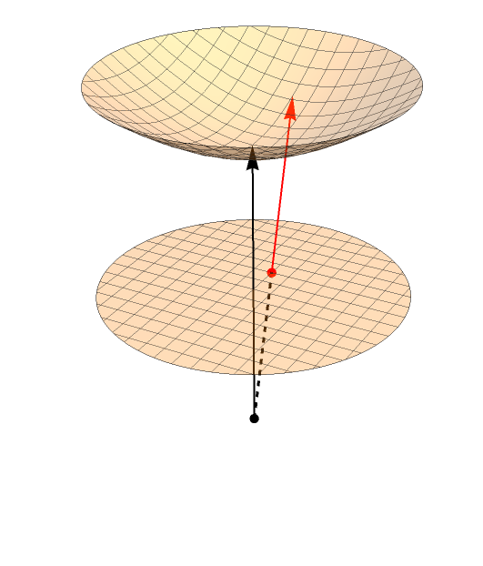
Figure 1: The Weierstrass map $\Xi:\mathrm{D}\rightarrow S^{+}$ coincides with the projection of $\mathrm{D}$ from the point $(-1,0,0)$ of three-dimensional Minkowski space, when the Poincaré disk is placed in the plane $X^{0}=0$. Notice that the conformal boundary of $\mathbb{D}$ is mapped to the circle at infinity of $S^{+}$. When $u\in\mathbb{D}$ approaches the conformal boundary, the 3-vector $\Xi(u)$ (shown in red) becomes lightlike.

The Weierstrass coordinates of any point $u\in D$ satisfy:

$$\left(\Xi^{0}(u)\right)^{\!2}-\left(\Xi^{1}(u)\right)^{\!2}-\left(\Xi^{2}(u)\right)^{\!2}=1~{}~{}\mathrm{and}~{}~{}\Xi^{0}(u)>0$$

and we have:

$$\Xi(u)=\Xi^{\mu}(u)E_{\mu}~{}~{},~{}~{}B=B^{\mu}E_{\mu}~{}~{},$$

where $E_{0}\stackrel{{\scriptstyle{\rm def.}}}{{=}}(1,0,0)$, $E_{1}\stackrel{{\scriptstyle{\rm def.}}}{{=}}(0,1,0)$ and $E_{2}\stackrel{{\scriptstyle{\rm def.}}}{{=}}(0,0,1)$.

The 3-vector parameterization.

The general Hesse function (83) reads:

$$\Lambda_{B}(u)=B_{\mu}\Xi^{\mu}(u)\!=\!\eta_{\mu\nu}B^{\mu}\Xi^{\nu}(u)\!=\!(B,\Xi(u))\!=\!B^{0}\Xi^{0}(u)-B^{1}\Xi^{1}(u)-B^{2}\Xi^{2}(u)~{}~{},$$ (87)

where we defined $B^{\mu}\stackrel{{\scriptstyle{\rm def.}}}{{=}}\eta^{\mu\nu}B_{\nu}$ and we combined the constants $B^{0}=B_{0}$, $B^{1}=-B_{1}$ and $B^{2}=-B_{2}$ into the 3-vector:

$$B\stackrel{{\scriptstyle{\rm def.}}}{{=}}(B^{0},B^{1},B^{2})=B^{\mu}E_{\mu}\in\mathbb{R}^{3}~{}~{}.$$

Notice the relation $\Xi_{\mu}(u)=(\Xi(u),E_{\mu})$. Since the Weierstrass coordinates form a basis of the space of Hesse functions, the linear map $\bm{\Lambda}:\mathbb{R}^{3}\stackrel{{\scriptstyle\sim}}{{\rightarrow}}\mathcal{S}(\mathbb{D})$ defined through:

$$\bm{\Lambda}(B)\stackrel{{\scriptstyle{\rm def.}}}{{=}}\Lambda_{B}~{}~{},~{}~{}\forall B\in\mathbb{R}^{3}~{}~{}$$ (88)

is an isomorphism of vector spaces from $\mathbb{R}^{3}$ to the space $\mathcal{S}(\mathbb{D})$.

Action of orientation-preserving isometries.

Since the Hesse equation is invariant under isometries of the scalar manifold, the group $\mathrm{PSU}(1,1)\simeq\mathrm{Iso}_{+}(\mathbb{D})$ of orientation-preserving isometries of $\mathbb{D}$ acts linearly on the space $\mathcal{S}(\mathbb{D})$ of Hesse functions through the representation $\mathcal{H}$ defined through:

$$\mathcal{H}(U)(\Lambda)\stackrel{{\scriptstyle{\rm def.}}}{{=}}\Lambda\circ\psi_{U}^{-1}~{},~{}~{}\forall U\in\mathrm{PSU}(1,1)$$

i.e.:

$$\mathcal{H}(U)(\Lambda)(u)=\Lambda(\psi_{U}^{-1}(u))~{}~{},~{}~{}\forall U\in\mathrm{PSU}(1,1)~{},~{}\forall u\in\mathrm{D}~{}~{}.$$

Here $\psi_{U}\in\mathrm{Iso}_{+}(\mathbb{D})$ is the orientation-preserving isometry of $\mathbb{D}$ corresponding to an element $U$ of $\mathrm{PSU}(1,1)$ (see Appendix B). The equivariance property (176) of the Weierstrass map gives:

$$\Xi_{\mu}(\psi_{U}(u))=(\mathrm{Ad}_{0}(U)(\Xi(u)),E_{\mu})=(\Xi(u),\mathrm{Ad}_{0}(U^{-1})(E_{\mu}))~{}~{}.$$

while equation (87) implies:

$$\Lambda_{B}(\psi_{U^{-1}}(u))=(B,\overline{\mathrm{Ad}}_{0}(U^{-1})(\Xi(u)))=(\overline{\mathrm{Ad}}_{0}(U)(B),\Xi(u))=\Lambda_{\overline{\mathrm{Ad}}_{0}(U)(B)}(u)~{}~{}.$$

This gives:

$$\mathcal{H}(U)(\Lambda_{B})=\Lambda_{\overline{\mathrm{Ad}}_{0}(U)(B)}~{}~{},~{}~{}\forall U\in\mathrm{PSU}(1,1)~{}~{},~{}~{}\forall B\in\mathbb{R}^{3}~{}~{},$$ (89)

i.e.:

$$\mathcal{H}(U)\circ\bm{\Lambda}=\bm{\Lambda}\circ\overline{\mathrm{Ad}}_{0}(U)~{}~{},~{}~{}\forall U\in\mathrm{PSU}(1,1)~{}~{},$$

showing that the linear isomorphism (88) is an equivalence of representations between $\mathcal{H}$ and ${\overline{\mathrm{Ad}}}_{0}$. As recalled in Appendix B, the representation $\overline{\mathrm{Ad}}_{0}$ (which is equivalent with the adjoint representation of $\mathrm{PSU}(1,1)$) preserves the Minkowski pairing (86). In fact, this representation defines an isomorphism of groups $\overline{\mathrm{Ad}}_{0}:\mathrm{PSU}(1,1)\stackrel{{\scriptstyle\sim}}{{\longrightarrow}}\mathrm{SO}_{o}(1,2)$, where $\mathrm{SO}_{o}(1,2)$ denotes the connected component of the identity of the Lorentz group, i.e. the group of proper and orthochronous Lorentz transformations in three dimensions.

Definition 5.1.

The Hesse function $\Lambda_{B}$ on the hyperbolic disk is called spacelike, timelike or lightlike if its parameter 3-vector $B\in\mathbb{R}^{3}$ is spacelike, timelike or lightlike, respectively. Similarly, $\Lambda_{B}$ is called future (resp. past) timelike or lightlike if it is timelike or lightlike and $B^{0}>0$ (respectively $B^{0}<0$).

5.2 Degenerate and non-degenerate Hesse functions

Definition 5.2.

A non-trivial Hesse function $\Lambda_{B}$ is called non-degenerate if $B^{0}\neq 0$ and degenerate if $B^{0}=0$.

Notice that a degenerate Hesse function is necessarily spacelike.

Rescaling non-degenerate Hesse functions.

Recall from (84) that $\sigma\!=\!\sqrt{B_{1}^{2}\!+\!B_{2}^{2}}$. When $B^{0}\neq 0$, we define:

$$\Delta=\frac{\sigma}{B^{0}}=\frac{\sqrt{B_{1}^{2}+B_{2}^{2}}}{B^{0}}~{}~{},~{}~{}b^{1}\stackrel{{\scriptstyle{\rm def.}}}{{=}}\frac{B^{1}}{B^{0}}=-\Delta\cos\theta_{0}~{},~{}~{}b^{2}\stackrel{{\scriptstyle{\rm def.}}}{{=}}\frac{B^{2}}{B^{0}}=-\Delta\sin\theta_{0}~{}~{}$$ (90)

and $\vec{b}\stackrel{{\scriptstyle{\rm def.}}}{{=}}(b^{1},b^{2})$, so that $B=B^{0}(1,b^{1},b^{2})=B^{0}(1,\vec{b})$ and $b_{1}^{2}+b_{2}^{2}=\Delta^{2}$. This allows us to write non-degenerate Hesse functions as:

$$\Lambda_{B}=B^{0}\lambda_{\vec{b}}~{}~{}(\mathrm{when}~{}~{}B^{0}\neq 0)~{},~{}$$

with

$$\lambda_{\vec{b}}\stackrel{{\scriptstyle{\rm def.}}}{{=}}\frac{1+\rho^{2}-2b^{1}x-2b^{2}y}{1-\rho^{2}}=\frac{1+\rho^{2}+2\Delta\rho\cos(\theta-\theta_{0})}{1-\rho^{2}}\stackrel{{\scriptstyle{\rm def.}}}{{=}}\lambda_{\Delta,\theta_{0}}~{}~{}.$$

In normal polar coordinates $(r,\theta)$ for the metric $\mathcal{G}$ we have:

$$\lambda_{\Delta,\theta_{0}}=\cosh(\beta r)+\Delta\sinh(\beta r)\cos(\theta-\theta_{0})~{}~{}.$$ (91)

Notice that a non-degenerate Hesse function is:

• timelike, iff $|\Delta|<1$.

• spacelike, iff $|\Delta|>1$.

• lightlike, iff $|\Delta|=1$, i.e. if $\Delta=+1$ (future lightlike) or $\Delta=-1$ (past lightlike).

When $\sigma\neq 0$, we have $\mathrm{sign}(B_{0})=\mathrm{sign}(\Delta)$. The shape of non-degenerate Hesse functions on $\mathbb{D}$ is illustrated in Figures 2, 3 and 4 for the case $B^{0}=1$ (i.e. $\Delta=\sigma\geq 0$) with $\theta_{0}=-\pi/2$, which gives $B=(1,0,\Delta)$ and:

$$\Lambda_{B}=\Lambda_{1,0,\Delta}=\frac{1+\rho^{2}-2\Delta y}{1-\rho^{2}}~{}~{}.$$

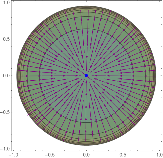
(a) $B=(1,0,0)$

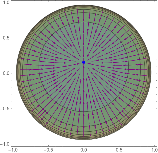
(b) $B=(1,0,0.3)$

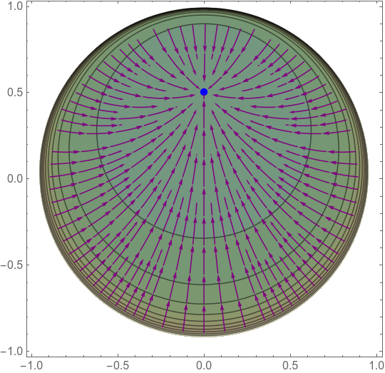
(c) $B=(1,0,0.8)$

Figure 2: Contour plot of $\Lambda:=\Lambda_{1,0,\Delta}$ for the non-degenerate timelike case ($\Delta<1$), where the gradient flow of $\Lambda$ is indicated by purple arrows. The values of $\Lambda$ decrease from lightest brown to darkest green. The critical point of $\Lambda$ is shown in blue. In this case, the level sets are hyperbolic circles centered at the critical point. From left to right, the figure shows the cases $\Delta=0,0.3,0.8$.

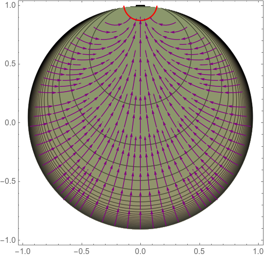
(a) $B=(1,0,1.01)$

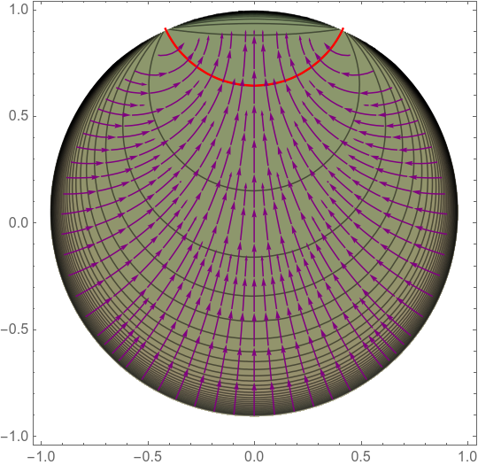
(b) $B=(1,0,1.1)$

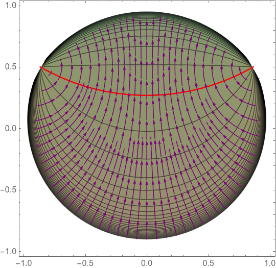
(c) $B=(1,0,2)$

Figure 3: Contour plot of $\Lambda:=\Lambda_{1,0,\Delta}$ for the non-degenerate spacelike case, where the gradient flow of $\Lambda$ is indicated by purple arrows. The values of $\Lambda$ decrease from lightest brown to darkest green. In this case, $\Lambda$ has no critical point but vanishes along the curve shown in red. In this case, the level sets are hypercycles with axis given by the vanishing locus of $\Lambda$. From left to right, the figure shows the cases $\Delta=1.01,1.1,2$.

Figure 4: Contour plot of $\Lambda_{1,0,1}$ (non-degenerate lightlike case with $\Delta=1$), where the gradient flow of $\Lambda$ is indicated by purple arrows. The values of $\Lambda$ decrease from lightest brown to darkest green. The point where $\Lambda$ tends to zero on the conformal boundary of the hyperbolic disk is shown in magenta. In this case, the level sets are horocycles centered at this ideal point.

Rescaling degenerate Hesse functions.

Non-trivial but degenerate (i.e. with $B^{0}=0$) Hesse functions have the form:

$$\Lambda_{0,B^{1},B^{2}}=\sigma\mu_{\theta_{0}}~{}~{},$$

where $B^{1}=-\sigma\cos\theta_{0}$, $B^{2}=-\sigma\sin\theta_{0}$ with $\sigma=\sqrt{B_{1}^{2}+B_{2}^{2}}>0$ and:

$$\mu_{\theta_{0}}\stackrel{{\scriptstyle{\rm def.}}}{{=}}\frac{2x\cos\theta_{0}+2y\sin\theta_{0}}{1-\rho^{2}}=\frac{2\rho}{1-\rho^{2}}\cos(\theta-\theta_{0})=\sinh(\beta r)\cos(\theta-\theta_{0})~{}~{}.$$ (92)

See Figure 5 for a contour plot of the function:

$$\Lambda_{0,0,1}=\mu_{-\pi/2}=-\frac{2y}{1-\rho^{2}}~{}~{}.$$ (93)

Remark 5.3.

When $\sigma\neq 0$, we have $\Delta\neq 0$ and $B^{0}=\frac{\sigma}{\Delta}$. In this case, we can write $\Lambda_{B}=\frac{\sigma}{\Delta}\lambda_{\Delta,\theta_{0}}$ and we have:

$$\lim_{\Delta\rightarrow\pm\infty}\frac{\lambda_{\Delta,\theta_{0}}(u)}{\Delta}=\mu_{\theta_{0}}(u)\Longrightarrow\lim_{\Delta\rightarrow\pm\infty}\Lambda_{B}(u)=\sigma\mu_{\theta_{0}}(u)~{}~{}.$$

Hence a non-degenerate Hesse function with $\sigma\neq 0$ point-wisely approximates the degenerate Hesse function with the same $\theta_{0}$ in the limits $\Delta\rightarrow\pm\infty$.

Remark 5.4.

It is easy to see that a Hesse function is separated in the coordinates $(r,\theta)$ or $(\rho,\theta)$ iff it is either degenerate or non-degenerate with $\Delta=0$. Hence $\Lambda_{B}$ separates in these coordinates only for $\Delta=0$ or in the limits $\Delta\rightarrow\pm\infty$.

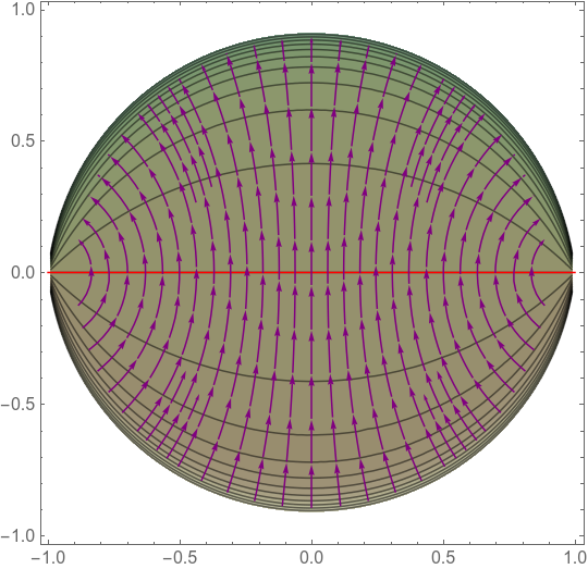
(a) $B=(0,0,1)$.

Figure 5: Contour plot of the degenerate spacelike Hesse function $\Lambda_{0,0,1}$, where the gradient flow of $\Lambda$ is indicated by purple arrows. The values of $\Lambda$ decrease from lightest brown to darkest green. The vanishing locus of $\Lambda$ is the horizontal segment shown in red. The level sets are hypercycles with axis given by the vanishing locus.

5.3 Critical points of Hesse functions

Definition 5.5.

A non-trivial Hesse function $\Lambda$ on the hyperbolic disk is called critical if it has at least one critical point, and non-critical if it has no critical points.

Proposition 5.6.

A non-trivial Hesse function $\Lambda_{B}$ on the hyperbolic disk is critical iff it is timelike (and hence non-degenerate). In this case, $\Lambda_{B}$ has exactly one critical point on $\mathrm{D}$, namely:

$$u_{c}=\left\{\begin{array}[]{ll}0&\mbox{if }\Delta=0\\ \frac{\sqrt{1-\Delta^{2}}-1}{\Delta}e^{\mathbf{i}\theta_{0}}&\mbox{if }0<|\Delta|<1\end{array}\right.~{}~{}$$ (94)

and the critical value of $\Lambda_{B}$ is given by:

$$\Lambda_{c}\stackrel{{\scriptstyle{\rm def.}}}{{=}}\Lambda(u_{c})=B_{0}\frac{1+\Delta^{2}}{\sqrt{1-\Delta^{2}}}~{}~{}.$$ (95)

Moreover, $u_{c}$ is an absolute minimum when $B_{0}>0$ (i.e. when $\Lambda_{B}$ is future-timelike) and an absolute maximum when $B_{0}<0$ (i.e. when $\Lambda_{B}$ is past-timelike).

Proof.

It is easy to see that a non-trivial degenerate Hesse function has no critical points in $\mathrm{D}$. If $\Lambda=\Lambda_{B}=B^{0}\lambda_{\Delta,\theta_{0}}$ is a non-degenerate Hesse function, then a counterclockwise rotation of the coordinates by an angle $\theta_{0}$ allows us to assume, without loss of generality, that $\theta_{0}=0$. Hence it suffices to study the critical points of the function:

$$\lambda:=\lambda_{\Delta,0}=\frac{1+x^{2}+y^{2}+2\Delta x}{1-x^{2}-y^{2}}~{}~{}.$$

The condition $(\mathrm{d}\lambda)(x,y)=0$ amounts to the system:

$$\Delta(1+x^{2}-y^{2})+2x=0$$

$$y(\Delta x+1)=0~{}~{}.$$ (96)

Multiplying the first equation by $y$ and the second equation by $x$ and subtracting the two gives:

$$\Delta y(1-x^{2}-y^{2})=0~{}~{},$$

which implies $\Delta y=0$ since $1-x^{2}-y^{2}>0$ for all points $u=x+\mathbf{i}y\in\mathrm{D}$. Using this, the second equation of (5.3) reduces to $y=0$, while the first equation becomes:

$$\Delta x^{2}+2x+\Delta=0~{}.$$ (97)

Distinguish the cases:

1. $\Delta=0$. Then $\Lambda$ is timelike, equation (97) gives $x=0$ and the only critical point of $\Lambda$ is $u_{c}=0$.

2. $\Delta\neq 0$ (hence $\Lambda$ is timelike or lightlike). Then (97) has real solutions iff $|\Delta|\leq 1$, in which case the two solutions are $x_{\pm}=\frac{-1\pm\sqrt{1-\Delta^{2}}}{\Delta}$. The case $\Delta=1$ leads to $x_{+}=x_{-}=1$, which is forbidden since the points $(x,y)=(1,0),(0,1)$ do not lie in the interior of the unit disk. Hence critical points inside $\mathrm{D}$ can exist only if $|\Delta|<1$, i.e. when $\Lambda$ is timelike. In this case, we have $|x_{+}|<1<|x_{-}|$, so the point $(x,y)=(x_{-},0)$ lies outside $\mathrm{D}$, while $(x,y)=(x_{+},0)$ lies inside $\mathrm{D}$. We conclude that $\Lambda$ is critical iff it is timelike, in which case the only critical point is at $u_{c}=\frac{\sqrt{1-\Delta^{2}}-1}{\Delta}$.

Since $\Lambda$ satisfies the Hesse equation $\mathrm{Hess}_{\mathcal{G}}(\Lambda)=\frac{3}{8}\Lambda\mathcal{G}$, it follows that its Hessian at $u_{c}$ is positive definite when $B_{0}>0$ and negative definite when $B_{0}<0$. Thus $u_{c}$ is a local minimum or maximum according to the sign of $B_{0}$. Substituting $u_{c}$ in the expression for $\Lambda$ gives (95).

The conclusion of the theorem now follows by performing a clockwise rotation of the coordinates by $\theta_{0}$, in order to restore the $\theta_{0}$-dependence in the position of the critical point. ∎

5.4 Level sets of Hesse functions

Relation (83) shows that the $\lambda$-level set $\{u\in\mathrm{D}\,|\,\Lambda_{B}(u)=\lambda\}$ of a non-trivial Hesse function $\Lambda_{B}$ has the equation:

$$(B_{0}+\lambda)(x^{2}+y^{2})+2B_{1}x+2B_{2}y+B_{0}-\lambda=0~{}~{}.$$ (98)

We distinguish the cases:

1. $\lambda\neq-B_{0}$. Then (98) takes the form:

   $$(x-x_{0})^{2}+(y-y_{0})^{2}=\frac{\lambda^{2}-(B,B)}{(B_{0}+\lambda)^{2}}~{}~{},$$ (99)

   where $x_{0}\stackrel{{\scriptstyle{\rm def.}}}{{=}}-\frac{B_{1}}{B_{0}+\lambda}$ and $y_{0}=-\frac{B_{2}}{B_{0}+\lambda}$. This equation has solutions only for $\lambda^{2}\geq(B,B)$, in which case it describes a Euclidean circle of radius $R\stackrel{{\scriptstyle{\rm def.}}}{{=}}\frac{\sqrt{\lambda^{2}-(B,B)}}{|B_{0}+\lambda|}$ centered at the point:

   $$u_{0}=x_{0}+\mathbf{i}y_{0}=\frac{B^{1}+\mathbf{i}B^{2}}{B^{0}+\lambda}~{}~{},$$

   which is reduced to this point for $\lambda^{2}=(B,B)$. The radius $R$ tends to infinity for $\lambda=-B_{0}$, in which case the circle degenerates to a line.

2. $\lambda=-B_{0}$. Then (98) takes the form:

   $$B_{1}x+B_{2}y=-B_{0}~{}~{}.$$

   Since $\Lambda_{B}$ is non-trivial, existence of solutions to this equation requires $B_{1}^{2}+B_{2}^{2}>0$ i.e. $\sigma>0$, in which case the equation describes a line in the $u$ plane which passes through the points $u_{1}=-\frac{B_{0}}{B_{1}}$ and $u_{2}=-\mathbf{i}\frac{B_{0}}{B_{2}}$ of the one point compactification of this plane. The relations $B_{1}=\sigma\cos\theta_{0}$ and $B_{2}=\sigma\sin\theta_{0}$ give:

   $$u_{1}=-\frac{1}{\Delta\cos\theta_{0}}~{}~{},~{}~{}u_{2}=-\frac{\mathbf{i}}{\Delta\sin\theta_{0}}~{}~{}.$$

   and bring the equation to the form:

   $$\rho\,\cos(\theta-\theta_{0})=-\frac{B_{0}}{\sigma}=-\frac{1}{\Delta}~{}~{},$$

   where the case $B_{0}=0$ is included for $\Delta\rightarrow\pm\infty$.

One can show that the Euclidean circles defined by equation (99) are contained inside $\mathrm{D}$ iff $B$ is lightlike and that they meet the Euclidean circle of radius one at one point when $B$ is timelike and at two points when $B$ is spacelike. It follows that the level sets of a timelike Hesse function are hyperbolic circles, while they are horocycles for a lightlike Hesse function and hypercycles for a spacelike Hesse function. These facts also follow more directly from the similar statements satisfied by the level sets of the three canonical Hesse functions discussed in Subsection 5.5, upon acting on those canonical forms with an orientation-preserving isometry of $\mathbb{D}$.

The vanishing locus of a Hesse function.

Let:

$$Z(\Lambda)\stackrel{{\scriptstyle{\rm def.}}}{{=}}\{u\in\mathrm{D}\,|\,\Lambda(u)=0\}$$

denote the set of zeroes of the Hesse function $\Lambda$. The proof of the following statement follows by inspection of equation (91).

Proposition 5.7.

A non-trivial Hesse function $\Lambda=\Lambda_{B}$ on the hyperbolic disk has zeroes iff it is spacelike, lightlike or degenerate. In this case, the vanishing locus of $\Lambda$ is a curve given by the following quadratic equation in Euclidean Cartesian coordinates on $\mathrm{D}$:

$$B_{0}(1+x^{2}+y^{2})+2B_{1}x+2B_{2}y=0~{}~{}.$$ (100)

Moreover:

• When $\Lambda$ is non-degenerate ($B_{0}\neq 0$), equation (100) is equivalent with:

  $$(x+b_{1})^{2}+(y+b_{2})^{2}=b_{1}^{2}+b_{2}^{2}-1(\geq 0)~{}~{},$$ (101)

  where $b_{1}=\frac{B_{1}}{B^{0}}$ and $b_{2}=\frac{B_{2}}{B^{0}}$. When $\Lambda$ is non-degenerate spacelike ($b_{1}^{2}+b_{2}^{2}>1$), the vanishing locus is a hypercycle which coincides with the intersection of $\mathrm{D}$ with a Euclidean circle of radius $\sqrt{b_{1}^{2}+b_{2}^{2}}$ centered at the point $u_{0}=-b_{1}-\mathbf{i}b_{2}$, which lies outside of $\mathrm{D}$. When $\Lambda$ is non-degenerate lightlike ($b_{1}^{2}+b_{2}^{2}=1$), the vanishing locus degenerates to the single point $u_{0}$, which lies on the conformal boundary of $\mathbb{D}$ (the unit Euclidean circle). In this case, the function $\Lambda$ tends to zero at this point of the conformal boundary.

• When $\Lambda$ is degenerate ($B_{0}=0$) and hence spacelike, the vanishing locus coincides with the intersection of $\mathrm{D}$ with the line obtained by rotating the $y$ axis counterclockwise by an angle equal to $\theta_{0}$.

5.5 The scalar potential determined by a Hesse function

In this subsection, we solve the $\Lambda$-$V$ equation (35) for a general Hesse function $\Lambda\in\mathcal{S}(\mathbb{D})$. We shall do so by combining representation-theoretic arguments with the method of characteristics. First, we notice that acting with an appropriate element $U$ of the group $\mathrm{PSU}(1,1)$ (and possibly rescaling by a constant) allows us to bring any non-trivial Hesse function $\Lambda$ to one of three specific canonical forms, depending on whether $\Lambda$ is timelike, spacelike or lightlike. We next determine the scalar potential $V$ by solving the $\Lambda$-$V$ equation for each of these three canonical choices of $\Lambda$. Finally, we act with the inverse of $U$ in order to recover the form of $V$ for a general Hesse function of timelike, spacelike or lightlike type. Equivalently, we write the scalar potentials for the three canonical cases in manifestly Lorentz-invariant form, which allows us to extend them to general Hesse functions of lightlike, spacelike and timelike type.

Reduction to canonical cases.

Let $V_{B}$ be the general solution of equation (35), where $\Lambda=\Lambda_{B}$ is a non-trivial Hesse function of $\mathbb{D}$. Relations (34) and (89) imply:

$$V_{B}(u)=V_{\overline{\mathrm{Ad}}_{0}(U)(B)}(\psi_{U}(u))~{}~{},~{}~{}\forall B\in\mathbb{R}^{3}~{}~{}\forall U\in\mathrm{PSU}(1,1)~{}~{}\forall u\in\mathrm{D}~{}~{}.$$ (102)

Moreover, the discussion of Subsection 3.5 shows that the general solution of the $\Lambda$-$V$ equation (35) is unchanged when one rescales $\Lambda$ by a non-zero constant. These observations imply the following:

• If $B$ is timelike or lightlike, there exists a proper orthochronous Lorentz transformation which brings $B$ to either of the following two forms:

  • $B^{\prime}=(C,0,0)$ with $C=\mathrm{sign}(B^{0})\sqrt{(B,B)}$ (when $B$ is timelike)

  • $B^{\prime}=(C,0,C)$ with $C=B^{0}$ (when $B$ is lightlike).

• If $B$ is spacelike, there exists a proper orthochronous Lorentz transformation (namely a spatial rotation) which brings $B$ to the form $B^{\prime}=(0,0,C)$, where $C=\sqrt{|(B,B)|}$.

Moreover, Remark 3.1 of Subsection 3.4 shows that we can rescale $\Lambda$ by $1/C$ without changing $V$. This allows us to further reduce to one of the thee canonical cases $B=B_{\mathrm{can}}\in\{(1,0,0),(1,0,1),(0,0,1)\}$. In each of the three cases, we have $B^{\prime}=CB_{\mathrm{can}}$ and:

$$V_{B^{\prime}}=V_{B_{\mathrm{can}}}=V_{B^{\prime}/C}$$

as well as:

$$V_{B}(u)=V_{B^{\prime}}(\psi_{U}(u))~{}~{},$$

where $B^{\prime}=\overline{\mathrm{Ad}}_{0}(U)(B)$ and $\overline{\mathrm{Ad}}_{0}(U)\in\mathrm{SO}_{0}(1,2)$ (with $U\in\mathrm{PSU}(1,1)$) is the corresponding Lorentz transformation.

In conclusion, we can reduce the problem of determining $V$ to the three canonical cases $B=B_{\mathrm{can}}\in\{(1,0,0),(0,0,1),(1,0,1)\}$, depending on whether $B$ is timelike, spacelike or lightlike. We next study each case in turn.

5.5.1 The case of timelike $\Lambda$

In this case, there exists a proper and orthochronous Lorentz transformation $\overline{\mathrm{Ad}}_{0}(U)$ which brings $B=(B^{0},B^{1},B^{2})$ to the form $B^{\prime}\stackrel{{\scriptstyle{\rm def.}}}{{=}}\overline{\mathrm{Ad}}_{0}(U)(B)=(C,0,0)=CB_{\mathrm{can}}$ with $C=\epsilon\sqrt{(B,B)}$ (where $\epsilon\stackrel{{\scriptstyle{\rm def.}}}{{=}}\mathrm{sign}(B_{0})$) and $B_{\mathrm{can}}=E_{0}=(1,0,0)$. We can take $U=U(t,a,0)\in\mathrm{PSU}(1,1)$, with $t>0$ and $a$ determined by the relations:

$$t=\operatorname{arccosh}\left[\frac{|B^{0}|}{\sqrt{(B,B)}}\right]~{},~{}\cos(a)=-\epsilon\frac{B^{1}}{\sqrt{B_{1}^{2}+B_{2}^{2}}}~{},~{}\sin(a)=\epsilon\frac{B^{2}}{\sqrt{B_{1}^{2}+B_{2}^{2}}}~{}~{}.$$ (103)

The canonical timelike Hesse function.

For $B=B_{\mathrm{can}}=(1,0,0)$, we have $\Delta=0$ and the corresponding Hesse function:

$$\Lambda_{B_{\mathrm{can}}}(u)=\Lambda_{1,0,0}(u)=\Xi^{0}(u)=\frac{1+\rho^{2}}{1-\rho^{2}}=\frac{2}{1-\rho^{2}}-1$$ (104)

has a single critical point located at $u_{c}=0$, which is an absolute minimum with $\Lambda_{1,0,0}(u_{c})=1$; moreover, $\Lambda_{1,0,0}$ tends to $\infty$ at the conformal boundary of $\mathbb{D}$. For each $\lambda\in[1,+\infty)$, the level set $\Lambda_{1,0,0}=\lambda$ is the Euclidean circle centered at the origin of radius $R_{\lambda}=\sqrt{\frac{\lambda-1}{\lambda+1}}$, which varies from $R_{1}=0$ to $R_{\infty}=1$ as $\lambda$ increases from $1$ to $+\infty$. The level sets are hyperbolic circles, since they are all contained inside $\mathrm{D}$.

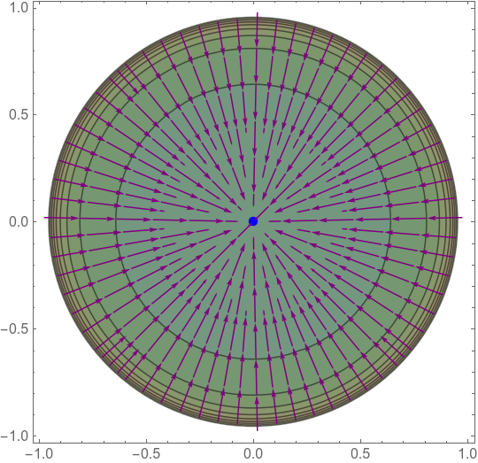
Figure 6: Contour plot of the canonical timelike Hesse function $\Lambda_{1,0,0}$. The values of the function decrease from lightest brown to darkest green. The critical point is shown as a blue dot. The gradient vector field is shown in purple. This coincides with Figure 2, which we recall here for convenience of the reader.

The scalar potential in the canonical timelike case.

The gradient flow equations of $\Lambda_{1,0,0}$ with respect to the metric $\mathcal{G}$ have the following form in polar Euclidean coordinates $(\rho,\theta)$:

$$\frac{\mathrm{d}\rho}{\mathrm{d}q}=-\beta^{2}\rho~{}~{},~{}~{}\frac{\mathrm{d}\theta}{\mathrm{d}q}=0~{}~{},$$ (105)

with the solution $\theta=\mathrm{const}$ and $\rho=e^{-\beta^{2}q}$, where $q\in(0,+\infty)$ and we chose the integration constant such that $\rho\rightarrow 1$ for $q\rightarrow 0$. Hence the gradient flow curves of $\Lambda_{1,0,0}$ are straight line segments flowing from the conformal boundary to the origin of $\mathbb{D}$ as $q$ varies from $0$ to $+\infty$ (see Figure 6). Let $\gamma_{\theta}$ denote the gradient flow line of polar angle $\theta$.

For $\Lambda=\Lambda_{1,0,0}$, relation (38) becomes:

$$\frac{\mathrm{d}q}{\mathrm{d}\lambda}=-\frac{1}{||\mathrm{d}\Lambda_{1,0,0}||_{\mathcal{G}}^{2}}=-\frac{1}{\beta^{2}\left(\lambda^{2}-1\right)}~{}~{}.$$

Along the gradient flow curve $\gamma_{\theta}$, we have:

$$\lambda=\frac{1+\rho^{2}}{1-\rho^{2}}\Longleftrightarrow\rho=\frac{\sqrt{\lambda-1}}{\sqrt{\lambda+1}}$$

and:

$$\int_{(\gamma)}^{\lambda}\frac{\lambda^{\prime}\mathrm{d}\lambda^{\prime}}{||\mathrm{d}\Lambda_{1,0,0}||_{\mathcal{G}}^{2}}=\frac{1}{2\beta^{2}}\log\left(\lambda^{2}-1\right)+\mathcal{C}(\theta)~{}~{},$$

where $\gamma(\lambda)=\rho\cos\theta+\mathbf{i}\rho\sin\theta$ and where $\mathcal{C}(\theta)$ is a constant of integration which can depend on $\theta$ in a $2\pi$-periodic manner. Relation (39) gives:

$$V_{B_{\mathrm{can}}}(\rho,\theta)=\omega(\theta)(\Lambda_{B_{\mathrm{can}}}(\rho)^{2}-1)=\omega(\theta)\frac{4\rho^{2}}{(1-\rho^{2})^{2}}~{}~{},$$ (106)

where $\omega(\theta)\stackrel{{\scriptstyle{\rm def.}}}{{=}}e^{2\beta^{2}\mathcal{C}(\theta)}$ is a positive $2\pi$-periodic smooth function of $\theta$.

Accidental visible symmetries in the canonical timelike case.

It is clear that $V_{1,0,0}$ is invariant under a continuous subgroup of $\mathrm{Iso}_{+}(\mathbb{D})\simeq\mathrm{PSU}(1,1)$ iff $\omega$ is independent of $\theta$, in which case $V_{1,0,0}$ is stabilized by the $\mathrm{U}(1)$ subgroup $\mathcal{R}$ corresponding to rotations of the disk around its origin (see Appendix B). The image of this subgroup in the adjoint representation $\overline{\mathrm{Ad}}_{0}$ coincides with the $\mathrm{SO}(2)$ group of spatial rotations which stabilizes the timelike 3-vector $B_{\mathrm{can}}=(1,0,0)$ in the Lorentz group. Hence the Hessian two-field model defined by $V_{1,0,0}$ also admits visible symmetries iff $\omega$ is independent of $\theta$, in which case the space of infinitesimal visible symmetries is one-dimensional and generated by the vector field $\partial_{\theta}$.

The scalar potential when $B=B^{\prime}=CB_{\mathrm{can}}$.

Recalling the relations $V_{B^{\prime}}=V_{B_{\mathrm{can}}}$ for $B^{\prime}=CB_{\mathrm{can}}$ as well as $\Lambda_{B_{\mathrm{can}}}=\Lambda_{B^{\prime}}/C$ (where $C=\epsilon\sqrt{(B^{\prime},B^{\prime})}$, relation (106) gives:

$$V_{B^{\prime}}(\rho,\theta)=\omega(\theta)\left[\frac{\Lambda_{B^{\prime}}(\rho)^{2}}{(B^{\prime},B^{\prime})}-1\right]~{}~{}(\mathrm{when}~{}~{}B^{\prime}_{1}=B^{\prime}_{2}=0)~{}~{}.$$ (107)

Lorentz-invariant form of the scalar potential.

When $B=B^{\prime}=CE_{0}$, the polar angle $\theta$ on the hyperbolic disk parameterizes the unit spacelike vector $n_{B}(u)\stackrel{{\scriptstyle{\rm def.}}}{{=}}\cos\theta E_{1}+\sin\theta E_{2}$ obtained by normalizing the projection $\Xi_{B}(u)$ of $\Xi(u)$ onto the spacelike plane orthogonal to $B$ (see Figure 7), which in this case is spanned by the three-vectors $E_{1}$ and $E_{2}$.

We have:

$$\Xi_{B}(u)=\Xi(u)-\frac{(B,\Xi(u))B}{(B,B)}~{}~{},$$

and $n_{B}(u)=\frac{\Xi_{B}(u)}{||\Xi_{B}(u)||_{E}}$, where the Euclidean norm of $\Xi_{B}(u)$ is given by:

$$||\Xi_{B}(u)||_{E}=\sqrt{-(\Xi_{B}(u),\Xi_{B}(u))}=\sqrt{\frac{(B,\Xi(u))^{2}}{(B,B)}-1}~{}~{},$$

where we used the relation $(\Xi(u),\Xi(u))=1$. Combining these formulas gives:

$$n_{B}(u)=\frac{(B,B)\Xi(u)-(B,\Xi(u))B}{\sqrt{(B,B)(B,\Xi(u))^{2}-(B,B)^{2}}}=\frac{(B,B)\Xi(u)-B\Lambda_{B}(u)}{\sqrt{(B,B)\Lambda_{B}(u)^{2}-(B,B)^{2}}}~{}~{}.$$ (108)

Since this relation is manifestly Lorentz invariant, it is valid not only for $B=B^{\prime}$, but also for any lightlike vector $B$. In particular, $\omega$ can be viewed as a function of the unit spacelike vector $n_{B}$ and relation (107) can be written in the manifestly Lorentz-invariant form:

$$V_{B}(u)=\omega(n_{B}(u))\left[\frac{\Lambda_{B}(u)^{2}}{(B,B)}-1\right]~{}~{}.$$ (109)

Direct computation using (87) gives:

$$\frac{\Lambda_{B}(u)^{2}}{(B,B)}-1=\frac{B_{1}^{2}(1+2x^{2}-2y^{2}+\rho^{4})+B_{2}^{2}(1-2x^{2}+2y^{2}+\rho^{4})+4B_{0}^{2}\rho^{2}+4B_{0}(1+\rho^{2})(B_{1}x+B_{2}y)+8B_{1}B_{2}xy}{(B,B)(1-\rho^{2})^{2}}~{}~{}.$$ (110)

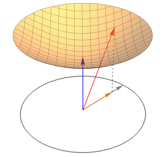
Figure 7: The unit spacelike vector $n_{B}(u)$ (shown in gray) determined by the unit timelike 3-vector $\Xi(u)$ (shown in red) and a timelike 3-vector $B$ (shown in blue); the projection $\Xi_{B}(u)$ is shown in orange. We also show the future sheet of the unit hyperboloid. As $u$ varies in $\mathrm{D}$, the vector $n_{B}(u)$ describes a circle of unit radius (shown in gray) contained in the spacelike plane orthogonal to $B$; one can think of the function $\omega$ as being defined on this circle. The figure shows the case when $B$ is future-pointing with $(B,B)=1$.

Remark 5.8.

Equation (102) shows that the general solution of (35) for a Hesse function of timelike parameter $B$ is obtained by acting on $\mathbb{D}$ with the $\mathrm{PSU}(1,1)$ transformation $U=U(t,a,0)$, with $a$ and $t$ given in (103):

$$V_{B}(u)=V_{B^{\prime}}(\psi_{U}(u))~{}~{},$$

where $B^{\prime}=\overline{\mathrm{Ad}}_{0}(U)(B)$. This amounts to replacing $(\rho,\theta)$ in expression (107) by polar semi-geodesic coordinates $({\tilde{\rho}},{\tilde{\theta}})$ centered at the critical point $u_{c}$ of $\Lambda_{B}$. In these new coordinates, the curves ${\tilde{\rho}}=\mathrm{const}$ (which coincide with the level sets of $\Lambda_{B}$) are hyperbolic circles with center $u_{c}$, while the curves ${\tilde{\theta}}=\mathrm{const}$ (which coincide with the gradient flow curves of $\Lambda_{B}$) are hyperbolic geodesics orthogonal to these hyperbolic circles and passing through $u_{c}$ (see Figure 2). We have:

$$V_{B}(x,y)=\omega({\tilde{\theta}}(x,y))\left[\frac{\Lambda_{B}(u)^{2}}{(B,B)}-1\right]~{}~{},$$ (111)

where:

$${\tilde{\theta}}(x,y)=\arg\left[\frac{\mathrm{sign}(B_{0})\,(B_{1}-\mathbf{i}B_{2})\,(x+\mathbf{i}y)+\left(|B_{0}|-\sqrt{(B,B)}\right)}{\left(|B_{0}|-\sqrt{(B,B)}\right)(x+\mathbf{i}y)+\mathrm{sign}(B_{0})\,(B_{1}+\mathbf{i}B_{2})}\right]~{}~{}.$$

Accidental visible symmetries in the general timelike case.

The potential (111) is stabilized by a non-trivial continuous subgroup of $\mathrm{PSU}(1,1)\simeq\mathrm{Iso}_{+}(\mathbb{D})$ (and hence the corresponding cosmological model also admits visible symmetries) iff the function $\omega$ is constant on the unit circle. In this case, the group of visible symmetries of the model coincides with the stabilizer of $V_{B}$ in $\mathrm{Iso}_{+}(\mathbb{D})$. This is an elliptic $\mathrm{U}(1)$ subgroup of $\mathrm{PSU}(1,1)$ which identifies with the stabilizer of the 3-vector $B$ under the adjoint representation:

$$\mathrm{Stab}_{\mathrm{PSU}(1,1)}(V_{B})=\mathrm{Stab}_{\mathrm{PSU}(1,1)}(B)\simeq\mathrm{U}(1)$$

and is conjugate to the canonical rotation subgroup $\mathcal{R}$ through the adjoint action of the group element $U=U(t,a,0)$:

$$\mathrm{Stab}_{\mathrm{PSU}(1,1)}(V_{B})=U^{-1}\mathcal{R}U~{}~{}.$$

5.5.2 The case of spacelike $\Lambda$

In this case, there exists $U=U(t,a,\frac{\pi}{2}-a)\in\mathrm{PSU}(1,1)$ such that $\overline{\mathrm{Ad}}_{0}(U)(B)=B^{\prime}=CB_{\mathrm{can}}$, where $B_{\mathrm{can}}=(0,0,1)=E_{2}$, $C=\sqrt{|(B,B)|}$ and the parameters $t,a$ are determined by the relations:

$$t=\!-\operatorname{arcsinh}\left(\!\frac{B^{0}}{\sqrt{|(B,B)|}}\!\right),~{}\sin(2a)\!=\!\frac{B^{1}}{\sqrt{B_{1}^{2}+B_{2}^{2}}}~{},~{}\cos(2a)\!=\!\frac{B^{2}}{\sqrt{B_{1}^{2}+B_{2}^{2}}}~{}.$$ (112)

The canonical spacelike Hesse function.

We have:

$$\Lambda_{B_{\mathrm{can}}}(u)=\Lambda_{0,0,1}(u)=-\Xi^{2}(u)=-\frac{2y}{1-\rho^{2}}~{}~{}.$$ (113)

This Hesse function has no critical point on $\mathrm{D}$ (see Figure 8). It vanishes along the horizontal segment $(-1,1)$ defined by $y=0$, being positive in the lower half plane (where it tends to $+\infty$ for $\rho\rightarrow 1$) and negative in the upper half plane (where it tends to $-\infty$ for $\rho\rightarrow 1$). For each $\lambda\in\mathbb{R}\setminus\{0\}$, the level set $\Lambda_{0,0,1}=\lambda$ is the intersection with $\mathrm{D}$ of the circle with center $u=\frac{\mathbf{i}}{\lambda}$ and radius $R_{\lambda}=\sqrt{1+\frac{1}{\lambda^{2}}}$, which is the hypercycle consisting of all points of $\mathbb{D}$ located at signed hyperbolic distance $d_{\lambda}=-\operatorname{arcsinh}(\lambda)$ from the axis $(-1,1)$.

Fermi coordinates with axis $(-1,1)$.

To describe the gradient flow lines of (113), it is convenient to pass to hypercyclic (a.k.a. Fermi) coordinates $(\tau,\sigma)$ with axis $(-1,1)$. These are semi-geodesic coordinates defined through:

$$\mathrm{sign}(y)\sigma\!\stackrel{{\scriptstyle{\rm def.}}}{{=}}\!\operatorname{arccosh}\sqrt{1\!+\!\frac{4y^{2}}{(1\!-\!\rho^{2})^{2}}}\!=\!\operatorname{arccosh}\sqrt{\Xi^{0}(u)^{2}\!-\!\Xi^{1}(u)^{2}}\!=\!\operatorname{arccosh}\sqrt{1\!+\!\Xi^{2}(u)^{2}}~{}~{}$$

$$\!\!\!\tau\!\stackrel{{\scriptstyle{\rm def.}}}{{=}}\!\operatorname{arcsinh}\!\left(\!\frac{2x}{\sqrt{4y^{2}\!+\!(1\!-\!\rho^{2})^{2}}}\!\right)\!\!=\!\operatorname{arcsinh}\!\left(\!\frac{\Xi^{1}(u)}{\sqrt{\Xi^{0}(u)^{2}\!-\!\Xi^{1}(u)^{2}}}\!\right)\!\!=\!\operatorname{arcsinh}\left(\!\frac{\Xi^{1}(u)}{\sqrt{1\!+\!\Xi^{2}(u)^{2}}}\!\right)~{}~{}$$

i.e.:

$$\Xi^{0}(u)=\cosh\sigma\cosh\tau~{}~{},~{}~{}\Xi^{1}(u)=\cosh\sigma\sinh\tau~{}~{},~{}~{}\Xi^{2}(u)=\sinh\sigma~{}~{}.$$

(a) $\Lambda_{0,0,1}$ on the hyperbolic disk.

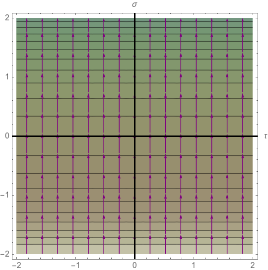
(b) $\Lambda_{0,0,1}$ in Fermi coordinates.

Figure 8: Contour plot of the canonical spacelike Hesse function $\Lambda_{0,0,1}$ and of its gradient flow. The values of the function decrease from lightest brown to darkest green. The figure to the left is Figure 5 recalled here for convenience of the reader. The vanishing locus of the function is the horizontal segment shown in red. The gradient vector field is shown in purple. The figure to the right shows only a portion of the $(\tau,\sigma)$-plane.

In Fermi coordinates, the metric $\mathcal{G}=G/\beta^{2}$ takes the form:

$$\mathrm{d}s^{2}_{\mathcal{G}}=\frac{1}{\beta^{2}}\left[\mathrm{d}\sigma^{2}+\cosh^{2}(\sigma)\mathrm{d}\tau^{2}\right]~{}~{}.$$

We have $\mathrm{sign}(\sigma(u))=\mathrm{sign}(y)=\mathrm{sign}(\Xi^{2}(u))$ and $\tau,\sigma\in\mathbb{R}$. The curves $\sigma=\mathrm{const}$ are hypercycles with axis given by the horizontal geodesic $(-1,1)$, while the curves $\tau=\mathrm{const}$ are hyperbolic geodesics orthogonal to these hypercycles (and hence also orthogonal to the $x$-axis). In these coordinates, the point $u=0$ corresponds to $(\tau,\sigma)=(0,0)$ while the conformal boundary of $\mathbb{D}$ corresponds to $\sigma^{2}+\tau^{2}\rightarrow\infty$, being mapped to a circle at infinity of the $(\tau,\sigma)$-plane. The $y$-axis $x=0$ corresponds to the line $\tau=0$ while the $x$-axis $y=0$ corresponds to the line $\sigma=0$. The squeeze transformation $T(t)\in\mathrm{PSU}(1,1)$ acts by:

$$\sigma\rightarrow\sigma~{}~{},~{}~{}\tau\rightarrow\tau+t~{}~{}.$$

In particular, the hypercycles with axis $(-1,1)$ are the orbits of the squeeze subgroup $\mathcal{T}$ of $\mathrm{PSU}(1,1)$ under the action of the latter on $\mathbb{D}$ by fractional transformations. Since $\Lambda_{0,0,1}=-\sinh(\sigma)$, the level sets of the canonical spacelike Hesse function coincide with the curves $\sigma=\mathrm{const}$, which are hypercycles located at signed hyperbolic distance $\sigma$ from the $x$-axis.

The scalar potential in the canonical spacelike case.

The gradient flow equations of $\Lambda_{0,0,1}$ take the following form in hypercyclic coordinates:

$$\frac{\mathrm{d}\sigma}{\mathrm{d}q}=\beta^{2}\cosh(\sigma)~{}~{},~{}~{}\frac{\mathrm{d}\tau}{\mathrm{d}q}=0~{}~{},$$

with the solution $\tau=\mathrm{const}$ and $\sigma=2\operatorname{arctanh}\left[\tan\left(\frac{\beta^{2}q}{2}\right)\right]=\operatorname{arcsinh}(\tan(q))$, where $q$ runs in the interval $(-\pi/2,\pi/2)$ and we chose $q=0$ to correspond to $\sigma=0$, i.e. to the unique point $u_{\tau}=\tanh(\tau/2)\in(-1,1)$ where the gradient flow curve corresponding to $\tau$ intersects the $x$-axis. We denote by $\gamma_{\tau}$ this gradient flow curve.

We have $\lambda=-\sinh(\sigma)$ and equation (38) becomes:

$$\frac{\mathrm{d}q}{\mathrm{d}\lambda}=-\frac{1}{||\mathrm{d}\Lambda_{0,0,1}||_{\mathcal{G}}^{2}}=-\frac{1}{\beta^{2}\left(\lambda^{2}+1\right)}~{}~{}.$$

Along the gradient flow curve $\gamma_{\tau}$ which passes through the point $u=x+\mathbf{i}y=\rho(\cos\theta+\mathbf{i}\sin\theta)\in\mathrm{D}$, we have:

$$\int_{(\gamma)}^{\lambda}\frac{\lambda^{\prime}\mathrm{d}\lambda^{\prime}}{||\mathrm{d}\Lambda_{0,0,1}||_{\mathcal{G}}^{2}}=\frac{1}{2\beta^{2}}\log\left(\lambda^{2}+1\right)+\mathcal{C}(\tau)~{}~{},$$

where $\gamma(\lambda)=u$ and where $\mathcal{C}(\tau)$ is a constant of integration which can depend on $\tau=\operatorname{arcsinh}\left(\frac{2x}{\sqrt{4y^{2}+(1-\rho^{2})^{2}}}\right)$. Equation (39) gives:

$$V_{B_{\mathrm{can}}}=\omega(\tau)\cosh^{2}(\sigma)=\omega(\tau)(1+\Lambda_{B_{\mathrm{can}}}(\sigma)^{2})~{}~{},$$ (114)

i.e.:

$$\!\!\!\!\!\!V_{B_{\mathrm{can}}}\!(u)\!=\!\omega(\tau)\!\left[1\!+\!\Lambda_{B_{\mathrm{can}}}(\sigma)^{2}\right]\!\!=\omega(\tau)\frac{1\!-\!2x^{2}\!+\!2y^{2}\!+\!\rho^{4}}{(1\!-\!\rho^{2})^{2}}~{}~{},$$ (115)

where $\omega\in\mathcal{C}^{\infty}(\mathbb{R})$ is a positive smooth real-valued function defined through $\omega(\tau)=e^{2\beta^{2}\mathcal{C}(\tau)}$.

Accidental visible symmetries in the canonical spacelike case.

It is clear that $V_{B_{\mathrm{can}}}$ is invariant under a continuous subgroup of isometries of $\mathbb{D}$ iff $\omega$ is independent of $\tau$, in which case the stabilizer of $V_{B_{\mathrm{can}}}$ coincides with the squeeze subgroup $\mathcal{T}$ of $\mathrm{PSU}(1,1)$. This corresponds to the group of boosts $\mathrm{Ad}_{0}(T(t))$ in the two-plane $(X^{0},X^{1})$ of the Minkowski space $\mathbb{R}^{1,2}$ (see Appendix B) which stabilize the 3-vector $B_{\mathrm{can}}\!=\!(0,0,1)$. This subgroup is isomorphic with $(\mathbb{R},+)$. Hence the Hessian two-field model defined by $V_{B_{\mathrm{can}}}$ also admits visible symmetries iff $\omega$ is independent of $\tau$, in which case the group of visible symmetries coincides with $\mathcal{T}$.

The scalar potential when $B=B^{\prime}=CB_{\mathrm{can}}$.

Recalling the relations $V_{B^{\prime}}=V_{B_{\mathrm{can}}}$ for $B^{\prime}=CB_{\mathrm{can}}$ as well as $\Lambda_{B_{\mathrm{can}}}=\Lambda_{B^{\prime}}/C$ (where $C=\sqrt{|(B^{\prime},B^{\prime})|}$), equation (115) gives:

$$V_{B^{\prime}}(\tau,\sigma)=\omega(\tau)\left[1+\frac{\Lambda_{B^{\prime}}(\sigma)^{2}}{|(B^{\prime},B^{\prime})|}\right]~{}~{}(\mathrm{when}~{}~{}B^{\prime}_{0}=B^{\prime}_{1}=0)~{}~{}.$$ (116)

Lorentz-invariant form of the scalar potential.

When $B=B_{\mathrm{can}}=(0,0,1)$, the hyperbolic angle $\tau$ parameterizes the unit timelike vector $n_{B}(u)=(\cosh\tau)E_{0}+(\sinh\tau)E_{1}$, which lies in the direction of the projection $\Xi_{B}(u)=\Xi^{0}(u)E_{0}+\Xi^{1}(u)E_{1}$ of $\Xi(u)$ onto the Minkowski plane orthogonal to $B$ (see Figure 9).

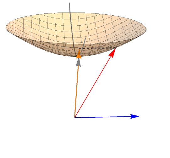
Figure 9: The unit timelike vector $n_{B}(u)$ (shown in gray) determined by the unit timelike vector $\Xi(u)$ and by the spacelike 3-vector $B$ (shown in blue). The timelike 3-vector $\Xi(u)$ is shown in red, while $\Xi_{B}(u)$ is shown in orange. As $u$ varies in $\mathrm{D}$, the vector $n_{B}(u)$ describes the hyperbola (shown in gray) obtained by intersecting the future sheet of the unit hyperboloid with the Minkowski plane orthogonal to $B$; one can think of the function $\omega$ as being defined on this hyperbola.

We have:

$$\Xi_{B}(u)=\Xi(u)+\frac{(B,\Xi(u))B}{|(B,B)|}~{}~{},$$

which gives:

$$(\Xi_{B}(u),\Xi_{B}(u))=1+\frac{(B,\Xi(u))^{2}}{|(B,B)|}~{}~{},$$

where we used the relation $(\Xi(u),\Xi(u))=1$. Thus:

$$n_{B}(u)\!=\!\frac{\Xi_{B}(u)}{\sqrt{\!(\Xi_{B}(u),\!\Xi_{B}(u))}}\!=\!\frac{|(B,\!B)|\,\Xi(u)\!+\!(B,\Xi(u))B}{\sqrt{\!(B,\!B)^{2}\!+\!|(B,\!B)|(B,\Xi(u))^{2}}}\!=\!\frac{|(B,\!B)|\,\Xi(u)\!+\!\Lambda_{B}(u)B}{\sqrt{\!(B,\!B)^{2}\!+\!|(B,\!B)|\Lambda_{B}(u)^{2}}}.$$ (117)

Since this relation is manifestly Lorentz invariant, it is valid not only for $B=B_{\mathrm{can}}$ but also for any spacelike vector $B$. In particular, $\omega$ can be viewed as a function of the unit timelike vector $n_{B}$ and relation (116) can be written in the manifestly Lorentz-invariant form:

$$V_{B}(u)=\omega(n_{B}(u))\left[1+\frac{\Lambda_{B}(u)^{2}}{|(B,B)|}\right]=-\omega(n_{B}(u))\left[\frac{\Lambda_{B}(u)^{2}}{(B,B)}-1\right]~{}~{},$$ (118)

where the quantity $\frac{\Lambda_{B}^{2}}{(B,B)}-1$ has the form given in (110).

Remark 5.9.

Equation (102) shows that the general solution of the $\Lambda$-$V$ equation (35) for a Hesse function of spacelike parameter $B$ is obtained by acting on $\mathbb{D}$ with the $\mathrm{PSU}(1,1)$ transformation $U=U(t,a,\pi/2-a)$, with $t$ and $a$ given in (112). This amounts to replacing $(\tau,\sigma)$ in expression (114) by hypercyclic coordinates $({\tilde{\tau}},{\tilde{\sigma}})$ with axis given by the vanishing locus $Z_{B}$ of the spacelike Hesse function $\Lambda_{B}$ (which is a hyperbolic geodesic). In the new coordinates, the curves ${\tilde{\sigma}}=\mathrm{const}$ (which coincide with the level sets of $\Lambda_{B}$) are hypercycles with axis $Z_{B}$ while the curves ${\tilde{\tau}}=\mathrm{const}$ (which coincide with the gradient flow curves of $\Lambda_{B}$) are hyperbolic geodesics orthogonal to these hypercycles (see Figure 3). We have:

$$V_{B}(x,y)=\omega({\tilde{\tau}}(x,y))\left[1+\frac{\Lambda_{B}(x,y)^{2}}{|(B,B)|}\right]~{}~{}.$$ (119)

with:

$$\sinh{\tilde{\tau}}(x,y)\!=\!\frac{2\sqrt{|(B,B)|}(B_{1}y\!-\!B_{2}x)}{\sqrt{(B_{1}^{2}\!+\!B_{2}^{2})\left[B_{1}^{2}(1\!+\!2x^{2}\!-\!2y^{2}\!+\!\rho^{4})\!+\!B_{2}^{2}(1\!-\!2x^{2}\!+\!2y^{2}\!+\!\rho^{4})\!+\!4B_{0}^{2}\rho^{2}\!+\!4B_{0}(1\!+\!\rho^{2})(B_{1}x\!+\!B_{2}y)\!+\!8B_{1}B_{2}xy\right]}}$$ (120)

Accidental visible symmetries in the general spacelike case.

It is clear that the potential (119) is stabilized by a non-trivial continuous subgroup of $\mathrm{Iso}_{+}(\mathbb{D})\simeq\mathrm{PSU}(1,1)$ (and hence the corresponding cosmological model also admits visible symmetries) iff the function $\omega$ is constant. In this case, the group of visible symmetries of the model coincides with the stabilizer of $V_{B}$. This is a hyperbolic subgroup isomorphic with $(\mathbb{R},+)$ which identifies with the stabilizer of the spacelike 3-vector $B$ under the adjoint representation:

$$\mathrm{Stab}_{\mathrm{PSU}(1,1)}(V_{B})=\mathrm{Stab}_{\mathrm{PSU}(1,1)}(B)\simeq(\mathbb{R},+)$$

and is conjugate to the squeeze subgroup $\mathcal{T}$ of $\mathrm{PSU}(1,1)$:

$$\mathrm{Stab}_{\mathrm{PSU}(1,1)}(V_{B})=U^{-1}\mathcal{T}U~{}~{},$$

where $U=U(t,a,\pi/2-a)$.

5.5.3 The case of lightlike $\Lambda$

In this case, there exists $U=U(0,a,0)\in\mathrm{PSU}(1,1)$ such that $\overline{\mathrm{Ad}}_{0}(U)(B)=(C,0,C)$, where $C=B^{0}$ and $a$ is determined by the relations:

$$\sin(2a)=\frac{B^{1}}{B^{0}}~{}~{},~{}~{}\cos(2a)=\frac{B^{2}}{B^{0}}~{}~{}.$$ (121)

Using (102), we can thus always reduce to the case $B=B^{\prime}=(C,0,C)$, while a rescaling of $\Lambda$ allows us to further reduce to the case $B=B_{\mathrm{can}}=(1,0,1)=E_{0}+E_{2}$.

The canonical lightlike Hesse function.

We have:

$$\Lambda_{B_{\mathrm{can}}}(u)=\Lambda_{1,0,1}(u)=\Xi^{0}(u)-\Xi^{2}(u)=\frac{\rho^{2}-2y+1}{1-\rho^{2}}~{}~{}.$$ (122)

This Hesse function has no critical points on $\mathrm{D}$ and is positive everywhere inside $\mathrm{D}$ (see Figures 10 and 4). It tends to $+\infty$ at all points of the conformal boundary of $\mathbb{D}$ except for the point $u_{0}=\mathbf{i}$, where it tends to zero. For any $\lambda\in(0,+\infty)$, the level set $\Lambda_{1,0,1}=\lambda$ is a horocycle with center $u_{0}=\mathbf{i}$.

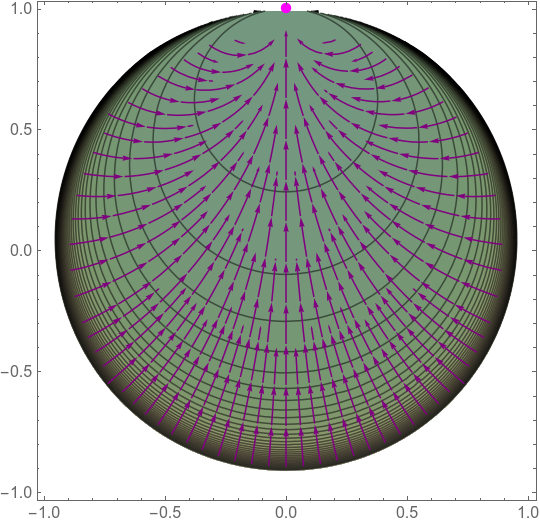
(a) $\Lambda_{1,0,1}$ on the hyperbolic disk.

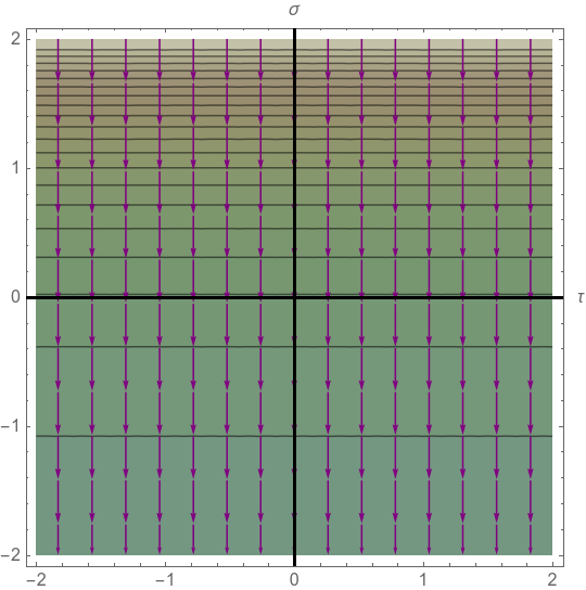
(b) $\Lambda_{1,0,1}$ in horocyclic coordinates.

Figure 10: Contour plot of the canonical lightlike Hesse function $\Lambda_{1,0,1}$ and of its gradient flow. The values of the function decrease from lightest brown to darkest green. In the figure on the left (which coincides with Figure 4), the single point on the conformal boundary of $\mathbb{D}$ where the function tends to zero is shown as a red dot. The gradient vector field is shown in purple. The figure to the right shows only a portion of the $(\tau,\sigma)$-plane.

Horocyclic coordinates centered at $\mathbf{i}$.

To describe the gradient flow of $\Lambda_{1,0,1}$, it is convenient to pass to horocyclic coordinates (which we again denote by $(\tau,\sigma)$) centered at $u=\mathbf{i}$. These are the hyperbolic polar geodesic coordinates defined through:

$$\sigma \stackrel{{\scriptstyle{\rm def.}}}{{=}} \log\left(\frac{\rho^{2}-2y+1}{1-\rho^{2}}\right)=\log\left[\Xi^{0}(u)-\Xi^{2}(u)\right]$$

$$\tau \stackrel{{\scriptstyle{\rm def.}}}{{=}} \frac{2x}{\rho^{2}-2y+1}=\frac{\Xi^{1}(u)}{\Xi^{0}(u)-\Xi^{2}(u)}~{}~{},$$ (123)

i.e.:

$$\Xi^{0}(u)=\frac{1}{2}\tau^{2}e^{\sigma}+\cosh\sigma~{}~{},~{}\Xi^{1}(u)=\tau e^{\sigma}~{}~{},~{}~{}\Xi^{2}(u)=\frac{1}{2}\tau^{2}e^{\sigma}-\sinh\sigma~{}~{}.$$

In particular, we have $\Lambda_{B_{\mathrm{can}}}(u)=\Xi^{0}(u)-\Xi^{2}(u)=e^{\sigma}$. In horocyclic coordinates, the metric $\mathcal{G}=G/\beta^{2}$ takes the form:

$$\mathrm{d}s^{2}_{\mathcal{G}}=\frac{1}{\beta^{2}}(\mathrm{d}\sigma^{2}+e^{2\sigma}\mathrm{d}\tau^{2})~{}~{}.$$

In these coordinates, the curves $\sigma=\mathrm{const}$ are the horocycles centered at $u=\mathbf{i}$ while the curves $\tau=\mathrm{const}$ are the geodesics normal to these horocycles, which have $\mathbf{i}$ as a limit point. In coordinates $(\tau,\sigma)$, the disk $\mathrm{D}$ is mapped to the entire plane $\mathbb{R}^{2}$, the conformal boundary of $\mathbb{D}$ corresponding to a circle at infinity. The origin of the disk corresponds to the origin of the $(\tau,\sigma)$-plane. The $y$-axis $x=0$ is mapped to the $\sigma$-axis $\tau=0$, while the Euclidean circle of radius $1/2$ centered at $u=\frac{\mathbf{i}}{2}$ (which is a horocycle of $\mathbb{D}$) is mapped to the $\tau$-axis $\sigma=0$. The interior of this horocycle is mapped to the half-plane $\sigma<0$, while its exterior is mapped to the half-plane $\sigma>0$; moreover, the limit $u\rightarrow\mathbf{i}$ corresponds to $\sigma\rightarrow-\infty$ and $\tau\rightarrow\pm\infty$, where $\tau\rightarrow+\infty$ if $u$ approaches $\mathbf{i}$ from the half-disk defined by $\mathrm{Re}u>0$ and $\tau\rightarrow-\infty$ if $u$ approaches $\mathbf{i}$ from the half-disk defined by $\mathrm{Re}u<0$. The horocycles with center $\mathbf{i}$ correspond to the curves $\sigma=\mathrm{const}$, while the hyperbolic geodesics which asymptote to $\mathbf{i}$ correspond to the curves $\tau=\mathrm{const}$. The shear transformation $P(\kappa)\in\mathrm{SU}(1,1)$ acts as:

$$\sigma\rightarrow\sigma~{}~{},~{}~{}\tau\rightarrow\tau+2\kappa~{}~{}.$$

In particular, the horocycles centered at $\mathbf{i}$ coincide with the orbits of the shear subgroup $\mathcal{P}$ under the action by fractional transformations. Since $\Lambda_{1,0,1}=e^{\sigma}$, the level sets of $\Lambda$ correspond to the curves $\sigma=\mathrm{const}$, which are horocycles passing through the point $\mathbf{i}$.

The scalar potential in the canonical lightlike case.

In horocyclic coordinates, the gradient flow equations of $\Lambda$ take the form:

$$\frac{\mathrm{d}\sigma}{\mathrm{d}q}=-\beta^{2}e^{\sigma}~{}~{},~{}~{}\frac{\mathrm{d}\tau}{\mathrm{d}q}=0~{}~{},$$

with the solution $\tau=\mathrm{const}$ and $\sigma=-\log\left[\beta^{2}q+1\right]$, where we chose the integration constant such that $q$ runs between $-1/\beta^{2}$ and $+\infty$, with $q\rightarrow-1/\beta^{2}$ corresponding to $\sigma\rightarrow+\infty$ and $q\rightarrow+\infty$ corresponding to $\sigma\rightarrow-\infty$. In the first limit, the gradient flow approaches a point on the conformal boundary of $\mathbb{D}$ where $\Lambda_{1,0,1}$ tends to plus infinity, while in the second limit the gradient flow approaches the ideal point $u=\mathbf{i}$ (where $\Lambda_{1,0,1}$ tends to zero). The value $q=0$ corresponds to the horocycle defined by the equation $\sigma=0$, which is the level set where $\Lambda_{1,0,1}=1$.

We have $\lambda=e^{\sigma}=\frac{\rho^{2}-2y+1}{1-\rho^{2}}$ and equation (38) becomes:

$$\frac{\mathrm{d}q}{\mathrm{d}\lambda}=-\frac{1}{||\mathrm{d}\Lambda_{1,0,1}||_{\mathcal{G}}^{2}}=-\frac{1}{\beta^{2}\lambda^{2}}~{}~{}.$$

Along a gradient flow curve $\gamma_{\tau}$ of $\Lambda_{1,0,1}$ which passes through the point $u=x+\mathbf{i}y=\rho(\cos\theta+\mathbf{i}\sin\theta)\in\mathrm{D}$, we have:

$$\int_{(\gamma)}^{\lambda}\frac{\lambda^{\prime}\mathrm{d}\lambda^{\prime}}{||\mathrm{d}\Lambda_{1,0,1}||_{\mathcal{G}}^{2}}=\frac{1}{\beta^{2}}\log(\lambda)+c(\tau)~{}~{},$$

where $\gamma(\lambda)\!=\!u$ and $c(\tau)$ is a constant of integration which can depend on $\tau\!=\!\frac{2x}{\rho^{2}-2y+1}$. Relation (39) gives:

$$V_{B_{\mathrm{can}}}(\tau,\sigma)=\omega(\tau)e^{2\sigma}=\omega(\tau)\Lambda_{B_{\mathrm{can}}}(\sigma)^{2}~{}~{},$$ (124)

i.e.:

$$V_{B_{\mathrm{can}}}(u)\!=\omega(\tau)e^{2\sigma}\!=\omega(\tau)\frac{\left(\rho^{2}\!-\!2\rho\sin\theta\!+\!1\right)^{2}}{(1-\rho^{2})^{2}}\!=\omega\!\left(\!\frac{2x}{\rho^{2}\!-\!2y\!+\!1}\!\right)\!\!\frac{\left(\rho^{2}\!-\!2y\!+\!1\right)^{2}}{(1-\rho^{2})^{2}}~{},$$ (125)

where the function $\omega\in\mathcal{C}^{\infty}(\mathbb{R})$ is defined through $\omega(\tau)=e^{2\beta^{2}c(\tau)}$.

Accidental visible symmetries in the canonical lightlike case.

It is clear that $V_{1,0,1}$ is invariant under a continuous subgroup of $\mathrm{PSU}(1,1)$ iff $\omega$ is independent of $\tau$, in which case the stabilizer of $V_{1,0,1}$ is the shear subgroup $\mathcal{P}$. Notice that $\mathcal{P}$ identifies with the stabilizer of $B_{\mathrm{can}}=(1,0,1)$ under the adjoint representation $\overline{\mathrm{Ad}}_{0}$ of $\mathrm{PSU}(1,1)$. Hence the Hessian two-field model with potential $V_{1,0,1}$ also admits visible symmetries iff $\omega$ is independent of $\tau$, in which case the group of visible symmetries coincides with the shear subgroup $\mathcal{P}$ of $\mathrm{PSU}(1,1)\simeq\mathrm{Iso}_{+}(\mathbb{D})$.

The scalar potential when $B=B^{\prime}=CB_{\mathrm{can}}$.

Recalling the relations $V_{B^{\prime}}=V_{B_{\mathrm{can}}}$ for $B^{\prime}=CB_{\mathrm{can}}$ as well as $\Lambda_{B_{\mathrm{can}}}=\Lambda_{B^{\prime}}/C$ (where $C=B^{\prime}_{0}$), relation (124) gives:

$$V_{B^{\prime}}(\tau,\sigma)=\omega(\tau)\frac{\Lambda_{B^{\prime}}(\sigma)^{2}}{(B^{\prime}_{0})^{2}}~{}~{}(\mathrm{when}~{}~{}B^{\prime}_{1}=0)~{}~{}.$$ (126)

Lorentz invariant form of the scalar potential.

Let $\Xi_{B}(u)$ denote the projection of the timelike vector $\Xi$ onto the light cone of $\mathbb{R}^{1,2}$, taken parallel to the lightlike vector $B$ (hence the 3-vector $\Xi_{B}(u)$ lies in the intersection of the light cone with the Minkowski plane spanned by $\Xi(u)$ and $B$ (see Figure 11). We have $\Xi_{B}(u)=\Xi(u)-\alpha B$, where $\alpha\in\mathbb{R}$ is determined by the condition $(\Xi_{B}(u),\Xi_{B}(u))=0$, which gives $\alpha=\frac{1}{2(B,\Xi(u))}$. Thus:

$$\Xi_{B}(u)=\Xi(u)-\frac{B}{2(B,\Xi(u))}~{}~{}.$$

Consider the lightlike 3-vector:

$$n_{B}(u)\stackrel{{\scriptstyle{\rm def.}}}{{=}}\frac{\Xi_{B}(u)}{(B,\Xi(u))}=\frac{2(B,\Xi(u))\Xi(u)-B}{2(B,\Xi(u))^{2}}=\frac{2\Lambda_{B}(u)\Xi(u)-B}{2\Lambda_{B}(u)^{2}}~{}~{},$$

which satisfies $(n_{B},B)=1$ and hence lies inside the affine plane $\Pi_{B}\subset\mathbb{R}^{1,2}$ defined by the equation $(X,B)=1$. We have $\Lambda_{B_{\mathrm{can}}}(u)=(B_{\mathrm{can}},\Xi(u))=e^{\sigma}$ and:

$$\Xi_{B_{\mathrm{can}}}(u)=e^{\sigma}\left(\frac{\tau^{2}+1}{2},\tau,\frac{\tau^{2}-1}{2}\right)~{}~{},$$

which gives:

$$n_{B_{\mathrm{can}}}(u)=\left(\frac{\tau^{2}+1}{2},\tau,\frac{\tau^{2}-1}{2}\right)~{}~{}.$$

This shows that the horocyclic coordinate $\tau$ parameterizes the light-like vector $n_{B_{\mathrm{can}}}$. We have $\Pi_{B_{\mathrm{can}}}=n_{0}+\Pi_{0}$, where the 3-vector $n_{0}=(1/2,0,-1/2)$ lies inside the light-cone and $\Pi_{0}$ is the linear plane defined by the equation $(X,B_{\mathrm{can}})=0$, i.e. $X^{0}=X^{2}$. The vectors $\epsilon_{1}=(0,1,0)$ and $\epsilon_{2}=(1,0,1)$ form a basis of this linear plane. Thus $n_{B_{\mathrm{can}}}(u)=n_{0}+\nu(u)$, where:

$$\nu(u)=\left(\frac{\tau^{2}}{2},\tau,\frac{\tau^{2}}{2}\right)=\tau\epsilon_{1}+\frac{\tau^{2}}{2}\epsilon_{2}\in\Pi_{0}~{}~{},$$

which shows that $n_{B_{\mathrm{can}}}(u)$ describes the parabola obtained by intersecting the light cone with the plane $\Pi_{B_{\mathrm{can}}}$. The apex of this parabola is the 3-vector $\nu_{0}$, which corresponds to $\tau=0$.

In particular, $\omega$ can be viewed as a function of the unit timelike vector $n_{B}$ and relation (126) can be written in the manifestly Lorentz-invariant form:

$$V_{B}(u)=\omega(B_{0}n_{B}(u))\frac{\Lambda_{B}(u)^{2}}{B_{0}^{2}}~{}~{}.$$ (127)

where:

$$\frac{\Lambda_{B}(u)^{2}}{B_{0}^{2}}=\frac{\left(B_{0}(1+\rho^{2})+2B_{1}x+2B_{2}y\right)^{2}}{B_{0}^{2}(1-\rho^{2})^{2}}~{}~{},$$ (128)

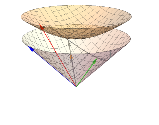
Figure 11: The lightlike vector $n_{B}(u)$ (shown in gray) determined by $\Xi(u)$ (shown in red) and by a lightlike 3-vector $B$ (shown in blue), where the 3-vector $\Xi_{B}(u)$ is shown in orange. As $u$ varies in $\mathrm{D}$, the vector $n_{B}(u)$ describes the parabola (shown in gray) obtained by intersecting the light cone with the plane defined in Minkowski 3-space by the equation $(X,B)=1$; one can think of the function $\omega$ as being defined on this parabola. The 3-vector $n_{0}$ corresponding to the apex of this parabola is shown in green. The figure shows the case when $B$ is future-lightlike.

Remark 5.10.

Equation (102) shows that the general solution of (35) for a Hesse function of lightlike parameter $B$ is obtained by acting on $\mathbb{D}$ with the $\mathrm{PSU}(1,1)$ transformation $U:=U(0,a,0)$, where $a$ is given in (121). This amounts to replacing $(\tau,\sigma)$ in expression (124) by horocyclic coordinates $({\tilde{\tau}},{\tilde{\sigma}})$ centered at the point $u_{0}\stackrel{{\scriptstyle{\rm def.}}}{{=}}\psi_{U^{-1}}(\mathbf{i})$ of the conformal boundary of $\mathbb{D}$ where the lightlike Hesse function $\Lambda_{B}$ tends to zero. In the new coordinates, the curves ${\tilde{\sigma}}=\mathrm{const}$ (which coincide with the level sets of $\Lambda_{B}$) are horocycles centered at $u_{0}$, while the curves ${\tilde{\tau}}=\mathrm{const}$ (which coincide with the gradient flow lines of $\Lambda_{B}$) are hyperbolic geodesics having $u_{B}$ as a limit point. This gives:

$$V_{B}(x,y)=\omega({\tilde{\tau}}(x,y))\frac{\Lambda_{B}(x,y)^{2}}{B_{0}^{2}}~{}~{},$$ (129)

where ${\tilde{\tau}}(x,y)\stackrel{{\scriptstyle{\rm def.}}}{{=}}\tau(\psi_{U}(x+\mathbf{i}y))$ is given by:

$${\tilde{\tau}}(x,y)=\frac{2(B_{1}y-B_{2}x)}{B_{0}(1+\rho^{2})+2B_{1}x+2B_{2}y}~{}~{}.$$ (130)

Accidental visible symmetries in the general lightlike case.

The potential (129) is stabilized by a non-trivial continuous subgroup of $\mathrm{PSU}(1,1)\simeq\mathrm{Iso}_{+}(\mathbb{D})$ (and hence the corresponding cosmological model also admits visible symmetries) iff the function $\omega$ is constant on $\mathbb{R}$. In this case, the stabilizer of $V_{B}$ is a parabolic subgroup isomorphic with $(\mathbb{R},+)$ which coincides with the stabilizer of the 3-vector $B$ under the adjoint representation:

$$\mathrm{Stab}_{\mathrm{PSU}(1,1)}(V_{B})=\mathrm{Stab}_{\mathrm{PSU}(1,1)}(B)\simeq(\mathbb{R},+)~{}~{}.$$

We have:

$$\mathrm{Stab}_{\mathrm{PSU}(1,1)}(B)=U^{-1}\mathcal{P}U~{}~{},$$

where $U=U(0,a,0)$.

5.6 Summary

The results of the previous subsections are summarized by the following theorem, which gives a complete classification of Hessian two-field models with scalar manifold $\mathbb{D}_{\beta}$:

Theorem 5.11.

The space of Hesse functions of the hyperbolic disk is 3-dimensional. A basis of this space is given by the classical Weierstrass coordinates $\Xi^{0},\Xi^{1},\Xi^{2}$ and the general Hesse function has the form:

$$\Lambda_{B}(u)=(B,\Xi(u))~{}~{}\forall u\in\mathrm{D}~{}~{},$$ (131)

where $\Xi=(\Xi^{0},\Xi^{1},\Xi^{2}):\mathrm{D}\rightarrow\mathbb{R}^{3}$ is the Weierstrass map, $B=(B^{0},B^{1},B^{2})\in\mathbb{R}^{3}$ is an arbitrary non-vanishing 3-vector parameter and $(~{},~{})$ is the Minkowski pairing of signature $(1,2)$ on $\mathbb{R}^{3}$. Moreover, the following statements hold for the weakly-Hessian two-field cosmological model whose scalar manifold is the disk $\mathbb{D}_{\beta}=(\mathrm{D},\mathcal{G})$, where $\mathcal{G}$ is the complete metric of constant negative curvature $K=-\frac{3}{8}$:

1. When $B$ is timelike, the two-field model with scalar manifold $\mathbb{D}_{\beta}$ admits the Hessian symmetry generated by (131) iff the scalar potential $V$ has the form:

   $$V_{B}(u)=\omega(n_{B}(u))\left[\frac{\Lambda_{B}(u)^{2}}{(B,B)}-1\right]~{}~{},$$ (132)

   where $\omega\in\mathcal{C}^{\infty}(\mathrm{S}^{1})$ is an arbitrary smooth function defined on the unit circle and $n_{B}(u)$ is the 3-vector given by:

   $$n_{B}(u)\!=\!\frac{(B,B)\Xi(u)\!-\!(B,\Xi(u))B}{\sqrt{(B,B)(B,\Xi(u))^{2}\!-\!(B,B)^{2}}}\!=\!\frac{(B,B)\Xi(u)-B\Lambda_{B}(u)}{\sqrt{(B,B)\Lambda_{B}(u)^{2}\!-\!(B,B)^{2}}}~{},$$ (133)

   which lies on the circle of unit radius located in the spacelike plane orthogonal to $B$ in $\mathbb{R}^{1,2}$ (see Figure 7). Here, the function $\omega$ is thought of as being defined on this circle. The model also admits visible symmetries iff $\omega$ is constant, in which case the group of visible symmetries is an elliptic subgroup of $\mathrm{PSU}(1,1)$ conjugate to the canonical rotation subgroup $\mathcal{R}\simeq\mathrm{U}(1)$; moreover, the group of visible symmetries coincides with the stabilizer of $B$ under the adjoint representation $\overline{\mathrm{Ad}}_{0}$ of $\mathrm{PSU}(1,1)$.

2. When $B$ is spacelike, the two-field model with scalar manifold $\mathbb{D}_{\beta}$ admits the Hessian symmetry generated by (131) iff its scalar potential $V$ has the form:

   $$V_{B}(u)=\omega(n_{B}(u))\left[\frac{\Lambda_{B}(u)^{2}}{|(B,B)|}+1\right]~{}~{},$$ (134)

   where $\omega\in\mathcal{C}^{\infty}(\mathbb{R})$ is an arbitrary smooth function defined on the real line and $n_{B}(u)$ is the unit timelike 3-vector given by:

   $$n_{B}(u)\!=\!\frac{|(B,B)|\,\Xi(u)+(B,\Xi(u))B}{\sqrt{(B,B)^{2}\!+\!|(B,B)|(B,\Xi(u))^{2}}}\!=\!\frac{|(B,B)|\,\Xi(u)+\Lambda_{B}(u)B}{\sqrt{(B,B)^{2}\!+\!|(B,B)|\Lambda_{B}(u)^{2}}}~{},$$ (135)

   which lies on the hyperbola obtained by intersecting the unit hyperboloid with the Minkowski plane orthogonal to $B$ (see Figure 9). Here, the function $\omega$ is thought of as being defined on this hyperbola. The explicit form of $V$ in Euclidean Cartesian coordinates is given in equations (119) and (120). The model also admits visible symmetries iff $\omega$ is constant, in which case the group of visible symmetries is a hyperbolic subgroup of $\mathrm{PSU}(1,1)$ conjugate to the canonical squeeze subgroup $\mathcal{T}\simeq(\mathbb{R},+)$; moreover, the group of visible symmetries coincides with the stabilizer of $B$ under the adjoint representation $\overline{\mathrm{Ad}}_{0}$ of $\mathrm{PSU}(1,1)$.

3. When $B$ is lightlike, the two-field model with scalar manifold $\mathbb{D}_{\beta}$ admits the Hessian symmetry generated by (131) iff its scalar potential $V$ has the form:

   $$V_{B}(u)=\omega(B_{0}n_{B}(u))\frac{\Lambda_{B}(u)^{2}}{B_{0}^{2}}~{}~{},$$ (136)

   where $\omega\in\mathcal{C}^{\infty}(\mathbb{R})$ is an arbitrary smooth function defined on the real line and $n_{B}(u)$ is the lightlike 3-vector given by:

   $$n_{B}(u)=\frac{2(B,\Xi(u))\Xi(u)-B}{2(B,\Xi(u))^{2}}=\frac{2\Lambda_{B}(u)\Xi(u)-B}{2\Lambda_{B}(u)^{2}}~{}~{},$$ (137)

   which lies on the parabola obtained by intersecting the light cone of $\mathbb{R}^{1,2}$ with the affine plane defined by the equation $(X,B)=1$ (see Figure 11). Here, the function $\omega$ is thought of as being defined on this parabola. The explicit form of $V$ in Euclidean Cartesian coordinates is given in equations (129) and (130). The model also admits visible symmetries iff $\omega$ is constant, in which case the group of visible symmetries is a parabolic subgroup of $\mathrm{PSU}(1,1)$ conjugate to the canonical shear subgroup $\mathcal{P}\simeq(\mathbb{R},+)$; moreover the group of visible symmetries coincides with the stabilizer of $B$ under the adjoint representation $\overline{\mathrm{Ad}}_{0}$ of $\mathrm{PSU}(1,1)$.

In each of the three cases, there exists an orientation-preserving isometry of the scalar manifold which brings the Hesse generator and the scalar potential to the corresponding canonical forms (see equations (104) and (124) for the timelike case, (113) and (115) for the spacelike case, (122) and (124) for the lightlike case).

Notice that $V_{B}$ depends only on the ray of the 3-vector $B$ in the projective Minkowski space $\mathbb{P}\mathbb{R}^{1,2}$. The explicit forms of the scalar potential in the three cases are as follows: $\bullet$ For timelike $B$ (i.e., for $(B,B)\stackrel{{\scriptstyle{\rm def.}}}{{=}}B_{0}^{2}-B_{1}^{2}-B_{2}^{2}>0$):

$$V_{B}(x,y)\!=\!\omega({\tilde{\theta}}(x,y))\,\frac{P}{(B,B)(1-\rho^{2})^{2}}~{}~{},$$ (138)

where:

$$P\!=\!(B_{1}^{2}+B_{2}^{2})(1\!+\!\rho^{4})\!+\!2(B_{1}^{2}-B_{2}^{2})(x^{2}\!-\!y^{2})\!+\!4B_{0}^{2}\rho^{2}\!+\!4B_{0}(1\!+\!\rho^{2})(B_{1}x\!+\!B_{2}y)\!+\!8B_{1}\!B_{2}xy$$ (139)

and:

$${\tilde{\theta}}(x,y)=\arg\!\left[\frac{\mathrm{sign}(B_{0})\,(B_{1}-\mathbf{i}B_{2})\,(x+\mathbf{i}y)+\left(|B_{0}|-\sqrt{(B,B)}\right)}{\left(|B_{0}|-\sqrt{(B,B)}\right)(x+\mathbf{i}y)+\mathrm{sign}(B_{0})\,(B_{1}+\mathbf{i}B_{2})}\right]~{}~{}.$$ (140)

$\bullet$ For spacelike $B$ (i.e., for $B_{0}^{2}-B_{1}^{2}-B_{2}^{2}<0$):

$$\!\!\!\!\!V_{B}(x,y)\!=\!\omega({\tilde{\tau}}(x,y))\,\frac{P}{|(B,B)|(1-\rho^{2})^{2}}~{},$$ (141)

where $P$ is given by (139) and:

$${\tilde{\tau}}(x,y)=\operatorname{arcsinh}\!\left[\frac{2\,\sqrt{|(B,B)|}\,(B_{1}y-B_{2}x)}{\sqrt{(B_{1}^{2}+B_{2}^{2})P}}\right]~{}.$$ (142)

$\bullet$ For lightlike $B$ (i.e., for $B_{0}^{2}-B_{1}^{2}-B_{2}^{2}=0$):

$$V_{B}(x,y)=\omega({\tilde{\tau}}(x,y))\,\frac{\left(B_{0}(1+\rho^{2})+2B_{1}x+2B_{2}y\right)^{2}}{B_{0}^{2}(1-\rho^{2})^{2}}~{}~{},$$ (143)

where:

$${\tilde{\tau}}(x,y)=\frac{2(B_{1}y-B_{2}x)}{B_{0}(1+\rho^{2})+2B_{1}x+2B_{2}y}~{}~{}.$$ (144)

6 Hessian models for the hyperbolic punctured disk

In this case, all Hesse functions are rotationally-invariant. Taking $C=1$ in (73), we find that the gradient vector field of the Hesse function $\Lambda=e^{-\beta r}$ has the following components in the rescaled normal polar coordinates $(r,\theta)$:

$$(\mathrm{grad}_{\mathcal{G}}\Lambda)^{r}=-\beta e^{-\beta r}$$

$$(\mathrm{grad}_{\mathcal{G}}\Lambda)^{\theta}=0~{}~{}.$$ (145)

Since $\rho=e^{-2\pi e^{\beta r}}$, the level sets of $\Lambda$ are Euclidean circles centered at the origin of $\mathbb{D}^{\ast}$, while the gradient flow curves are half lines passing through the origin (which corresponds to $r\rightarrow+\infty$); the gradient curves flow from the outer component of the conformal boundary of $\mathbb{D}^{\ast}$, which is the Euclidean circle of radius $1$ corresponding to $r\rightarrow-\infty$. The gradient flow equations of $\Lambda$:

$$\frac{\mathrm{d}r}{\mathrm{d}q}=\beta e^{-\beta r}~{}~{},~{}~{}\frac{\mathrm{d}\theta}{\mathrm{d}q}=0$$

give $\theta=\mathrm{const}$ and:

$$e^{\beta r}=1+\beta^{2}q~{}\Longleftrightarrow~{}q=\frac{1}{\beta^{2}}\left(e^{\beta r}-1\right)~{}~{},$$ (146)

where we chose the constant of integration such that $r|_{q=0}=0$, i.e. such that $\rho|_{q=0}=e^{-2\pi}$; this amounts to using the Euclidean circle $C_{0}$ of radius $\rho_{0}\stackrel{{\scriptstyle{\rm def.}}}{{=}}e^{-2\pi}$ (which has unit hyperbolic circumference) as a section $\mathcal{Q}$ for the gradient flow. We have:

$$\int_{0}^{q}\Lambda(\gamma(q^{\prime}))\mathrm{d}q^{\prime}=\int_{0}^{q}e^{-\beta r(q^{\prime})}\mathrm{d}q^{\prime}=\int_{0}^{q}\frac{1}{1+\beta^{2}q^{\prime}}\mathrm{d}q^{\prime}=\frac{1}{\beta^{2}}\log\left(1+\beta^{2}q\right)=\frac{1}{\beta}r~{}~{}.$$

Relation (37) gives:

$$V=\omega(\theta)e^{-2\beta r}=\omega(\theta)e^{-\sqrt{\frac{3}{2}}r}=\omega(\theta)\frac{4\pi^{2}}{(\log\rho)^{2}}~{}~{},$$ (147)

where we used equation (74) and we defined $\omega(\theta)\stackrel{{\scriptstyle{\rm def.}}}{{=}}V(r,\theta)|_{r=0}=V(\rho,\theta)|_{\rho=\rho_{0}}$. Notice that $\omega$ (which can be viewed as a smooth function defined on the unit circle) can be identified with the restriction of $V$ to the circle $C_{0}$, which plays the role of section for the gradient flow of $\Lambda$.

The space of Killing vector fields of $\mathbb{D}^{\ast}$ is generated by $\partial_{\theta}$, which is a visible symmetry iff $\partial_{\theta}V=0$, which amounts to the condition that $\omega$ be independent of $\theta$. The following statement summarizes these results:

Theorem 6.1.

The space of Hesse functions of the hyperbolic punctured disk is one-dimensional, being generated by:

$$\Lambda=e^{-\beta r}=\frac{2\pi}{|\log\rho|}~{}~{},$$ (148)

where $(r,\theta)$ are polar semi-geodesic coordinates for the complete metric $\mathcal{G}$ of Gaussian curvature $-\beta^{2}=-3/8$. For $C\neq 0$, this Hesse function generates a Hessian symmetry of the two-field cosmological model with scalar manifold $\mathbb{D}^{\ast}_{\beta}$ iff the scalar potential has the form:

$$V(r,\theta)=\omega(\theta)e^{-2\beta r}=\omega(\theta)\frac{4\pi^{2}}{(\log\rho)^{2}}~{},$$ (149)

where $\omega\in\mathcal{C}^{\infty}(\mathrm{S}^{1})$ is an arbitrary smooth function defined on the unit circle (viewed as a $2\pi$-periodic smooth function of the polar angle $\theta$). In this case, the corresponding Hessian symmetry is generated by the vector field:

$$X_{\Lambda}=\frac{\Lambda}{\sqrt{a}}\partial_{a}-\frac{4}{a^{3/2}}\mathrm{grad}\Lambda=e^{-\beta r}\Big{(}\frac{1}{\sqrt{a}}\partial_{a}+\frac{4\beta}{a^{3/2}}\partial_{r}\Big{)}=2\pi\left[\frac{1}{\sqrt{a}|\log\rho|}\partial_{a}-4\beta^{2}\frac{\rho}{a^{3/2}}\partial_{\rho}\right]~{}~{}.$$

When $\omega$ is not constant, the space of Noether symmetries of such a model is one-dimensional and coincides with the space of Hessian symmetries, being spanned by the vector field $X_{\Lambda}$. When $\omega$ is constant, the model also admits visible symmetries, whose generators form a one-dimensional vector space spanned by $\partial_{\theta}$. In this special case, the space of Noether symmetries is two-dimensional and admits a basis given by the vector fields $X_{\Lambda}$ and $\partial_{\theta}$.

The radial profiles of $\Lambda$ and $V$ are plotted in Figure 12.

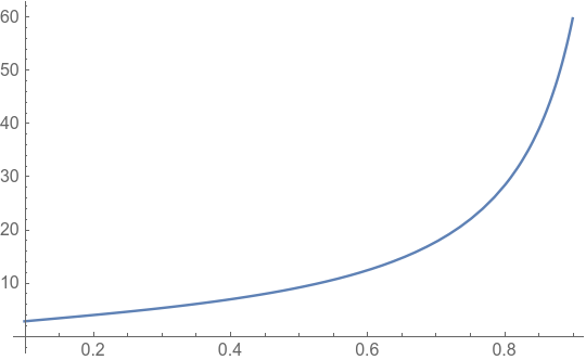
(a) Plot of $\Lambda(\rho)/C$.

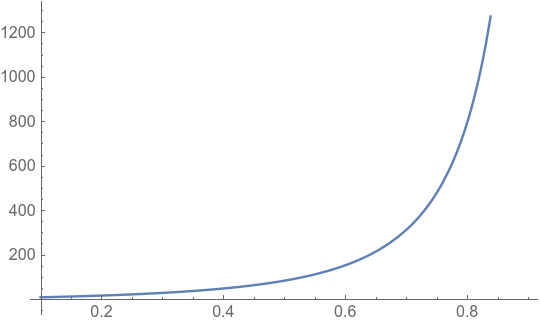
(b) Plot of $V(\rho,\theta)/\omega(\theta)$.

Figure 12: Plot of the radial profiles of $\Lambda/C$ and $V$ for the hyperbolic punctured disk.

7 Hessian models for the hyperbolic annuli

In this case, all Hesse functions are rotationally-invariant. Using (79) with $C\!=\!1$, we find that the gradient vector field of $\Lambda\!=\!\sinh(\beta r)$ has the following components in normal polar coordinates $(r,\theta)$ for the metric $\mathcal{G}$ of Gaussian curvature $-\beta^{2}$:

$$(\mathrm{grad}_{\mathcal{G}}\Lambda)^{r}=\beta\cosh(\beta r)$$

$$(\mathrm{grad}_{\mathcal{G}}\Lambda)^{\theta}=0~{}~{}.$$ (150)

The gradient flow equations of $\Lambda$:

$$\frac{\mathrm{d}r}{\mathrm{d}q}=-\beta\cosh(\beta r)~{}~{},~{}~{}\frac{\mathrm{d}\theta}{\mathrm{d}q}=0$$ (151)

give $\theta=\theta_{0}=\mathrm{const}$ and:

$$\tanh(\beta r/2)=-\tan(\beta^{2}q/2)~{}~{},$$ (152)

where we chose the gradient flow parameter such that $r|_{q=0}=0$ (i.e. $\rho|_{q=0}=1$) and we used the formula:

$$\int\frac{\mathrm{d}r}{\cosh(\beta r)}=\frac{2}{\beta}\arctan\left[\tanh\left(\frac{\beta r}{2}\right)\right]+\mathrm{const}~{}~{}.$$

In this case, the section $\mathcal{Q}$ for the gradient flow of $\Lambda$ is the Euclidean circle $C_{1}$ of radius $\rho=1$ (which separates the two funnel regions of $\mathbb{A}(R)$). Using (151), more precisely:

$$\mathrm{d}q^{\prime}=-\frac{1}{\beta\cosh(\beta r^{\prime})}\mathrm{d}r^{\prime}~{}~{},$$

gives:

$$\int_{0}^{q}\Lambda(\gamma(q^{\prime}))\mathrm{d}q^{\prime}=\int_{0}^{q}\sinh(\beta r(q^{\prime}))\mathrm{d}q^{\prime}=-\frac{1}{\beta}\int_{0}^{r}\tanh(\beta r^{\prime})\mathrm{d}r^{\prime}=-\frac{1}{\beta^{2}}\log\left[\cosh(\beta r)\right]~{}~{}.$$

Hence, relation (37) implies:

$$V(r,\theta)=\omega(\theta)e^{2\log\left[\cosh(\beta r)\right]}=\omega(\theta)\cosh^{2}(\beta r)=\frac{\omega(\theta)}{\cos^{2}\left(\frac{\pi}{\mu}|\log\rho|\right)}~{}~{},$$ (153)

where we defined $\omega(\theta)\stackrel{{\scriptstyle{\rm def.}}}{{=}}V(r,\theta)|_{r=0}=V(\rho,\theta)|_{\rho=1}$. Notice that $\omega$ can be viewed as a smooth function defined on the unit circle, which identifies with the restriction of $V$ to the Euclidean circle $C_{1}$.

The space of Killing vector fields of $\mathbb{A}(R)$ is generated by $\partial_{\theta}$. The latter is a visible symmetry iff $\partial_{\theta}V=0$, which amounts to the condition that $\omega$ be independent of $\theta$. Summarizing everything, we have:

Theorem 7.1.

The space of Hesse functions of the hyperbolic annulus $\mathbb{A}(R)$ is one-dimensional, being generated by the function:

$$\Lambda=\sinh(\beta r)=\tan\left(\frac{\pi}{\mu}\log\rho\right)~{}~{},$$ (154)

where $(r,\theta)$ are polar semi-geodesic coordinates for the complete metric $\mathcal{G}$ of Gaussian curvature $-\beta^{2}=-3/8$. This function generates a Hessian symmetry of the two-field cosmological model with scalar manifold $\mathbb{A}_{\beta}(R)$ iff the scalar potential has the form:

$$V(r,\theta)=\omega(\theta)\cosh^{2}(\beta r)=\frac{\omega(\theta)}{\cos^{2}\left(\frac{\pi}{\mu}|\log\rho|\right)}~{}~{},$$ (155)

where $\omega\in\mathcal{C}^{\infty}(\mathrm{S}^{1})$ is an arbitrary smooth function defined on the unit circle (viewed as a $2\pi$-periodic smooth function of the polar angle $\theta$). In this case, the corresponding Hessian symmetry is generated by the vector field:

$$X_{\Lambda} = \frac{\Lambda}{\sqrt{a}}\partial_{a}-\frac{4}{a^{3/2}}\mathrm{grad}\Lambda=\frac{\sinh(\beta r)}{\sqrt{a}}\partial_{a}-4\beta\frac{\cosh(\beta r)}{a^{3/2}}\partial_{r}$$

$$= \frac{\tan\left(\frac{\pi}{\mu}\log\rho\right)}{\sqrt{a}}\partial_{a}-\left(\frac{4\beta^{2}\mu}{\pi}\right)\frac{\rho}{a^{3/2}}\partial_{\rho}~{}~{}.$$

When $\omega$ is not constant, the space of Noether symmetries of such a model is one-dimensional and coincides with the space of Hessian symmetries, being spanned by the vector field $X_{\Lambda}$. When $\omega$ is constant on $\mathrm{S}^{1}$, the model also admits visible symmetries, whose generators form a one-dimensional linear space spanned by $\partial_{\theta}$. In this case, the space of Noether symmetries is two-dimensional and admits a basis given by the vector fields $X_{\Lambda}$ and $\partial_{\theta}$.

The radial profiles of $\Lambda$ and $V$ are plotted in Figure 12 for the hyperbolic annulus of modulus $\mu=2\log 2$ (i.e. $R=2$).

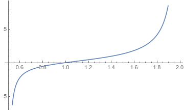
(a) Plot of $\Lambda(\rho)/C$

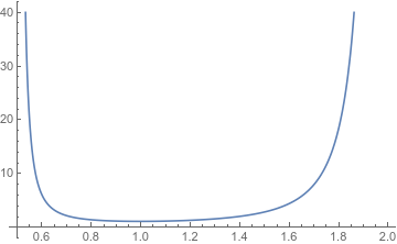
(b) Plot of $V(\rho,\theta)/\omega(\theta)$

Figure 13: Plot of the radial profiles of $\Lambda/C$ and $V$ on the hyperbolic annulus of modulus $\mu=2\log 2$ (i.e. for $R=2$). In this case $\rho$ runs from $1/2$ to $2$.

8 Conclusions and further directions

We studied time-independent Noether symmetries in two-field cosmological models, showing that any such symmetry decomposes as a direct sum of a visible and a Hessian symmetry. While visible symmetries correspond to those isometries of the scalar manifold which preserve the scalar potential (and in this sense are “obvious” symmetries), Hessian symmetries are “hidden” in the sense that they are not apparent upon direct inspection. We showed that any Hessian symmetry is determined by a generating function $\Lambda$. The latter is a Hesse function of the scalar manifold $(\Sigma,G=\frac{3}{8}\mathcal{G})$, i.e. a real-valued function $\Lambda$ defined on $\Sigma$ and which obeys the Hesse equation of $(\Sigma,G)$ (a certain second order linear PDE for $\Lambda$ which involves the rescaled scalar manifold metric $G=\frac{3}{8}\mathcal{G}$). Moreover, the scalar potential $V$ of a model which admits a Hessian symmetry must obey the $\Lambda$-$V$ equation (a certain first order PDE for $V$ which involves $\Lambda$ and $\mathcal{G}$).

When the scalar manifold metric $\mathcal{G}$ is rotationally invariant, we showed that the two-field model admits a Hessian symmetry iff $\Sigma$ is a disk, a punctured disk or an annulus and $\mathcal{G}$ is a complete metric of Gaussian curvature $K=-\frac{3}{8}$, i.e. iff the model is an elementary two-field $\alpha$-attractor in the sense of reference elem , for the particular value $\alpha=8/9$ of the $\alpha$-parameter. In all cases, we determined the explicit general form of the scalar potential $V$ which is compatible with a given Hessian symmetry. We also discussed the special cases when such a model also admits a visible symmetry. Finally, we discussed the integral of motion of a Hessian symmetry — showing that it allows one to simplify the computation of the number of e-folds along cosmological trajectories.

The present paper opens up a few avenues for further research, some of which we plan to address in future work. First, we will show in a separate paper (using a more general framework) that the classification of Hessian models given in this paper is in fact valid without assuming rotational invariance of the scalar manifold metric. One can also show that the existence of a Hessian symmetry enables an effective one-field model description (as far as one is concerned with determining classical trajectories) for each fixed value of the corresponding integral of motion, a fact which has interesting implications for contact with observational data. Furthermore, the approach of the present paper can be extended to the study of symmetries in $n$-field cosmological models, for which it leads to a rich mathematical theory.

Another direction for future studies concerns the possible embeddings of such models into supergravity or string theories, where we expect them to arise as points of “enhanced symmetry” in the moduli spaces of various compactifications. It is also worth noting that in recent years there have been a number of investigations of novel behavior arising from non-trivial angular motion in two-field models on the hyperbolic disk (see references KL7 ; LWWYA ; DFRSW ; ARB ; MM ; CRS ; GSRPR ; TB ). Our results provide a vast arena for even deeper and more involved studies along those lines. Indeed, having a Noether symmetry enables one to find exact (as opposed to numerical) solutions of the cosmological equations of motion, in particular obtaining explicit expressions for the Hubble parameter as a function of time; see ABL (as well as CDeF and references therein, in the context of extended theories of gravity). This would facilitate investigating with analytical means a variety of new regimes of expansion. It would be especially interesting to find new non-slow-roll inflationary regimes, which are perturbatively stable and produce a nearly scale-invariant spectrum of fluctuations (as needed for consistency with observations). Even for single-field models, such a regime was established only relatively recently MSY ; ASW . For two-field models the problem is more challenging, but may also present new opportunities. As already mentioned, the presence of a Noether symmetry in the class of models, considered in the present paper, may prove to be of great help in that regard.

It would also be interesting to explore whether the present work can be useful for a wider program (which was touched upon briefly in reference flows ) aimed at studying multifield cosmological models with methods from the geometric theory of dynamical systems (see Palis for an introduction). As pointed out in flows , the dynamics of such models is quite rich and in particular it is amenable to certain methods originating in asymptotic analysis. It would be interesting to gain a deeper understanding of the simplifications which the presence of a Hessian symmetry may afford in that context. We hope to report on these and related problems in future work.

Appendix A Geometric formulation of the method of characteristics

In this appendix, we recall the geometric formulation of the method of characteristics for solving a first order PDE of the form:

$$\iota_{X}\mathrm{d}f=g~{}~{}$$ (156)

for an unknown smooth function $f\in\mathcal{C}^{\infty}(\Sigma)$ defined on a manifold $\Sigma$, where $X$ is a vector field given on $\Sigma$, $g\in\mathcal{C}^{\infty}(\Sigma)$ is a given function and $\iota_{X}$ denotes contraction with $X$. The method relies on the observation that the identity $L_{X}=\mathrm{d}\iota_{X}+\iota_{X}\mathrm{d}$ allows us to write (156) in the equivalent form:

$$L_{X}f=g~{}~{},$$ (157)

where $L_{X}$ is the Lie derivative with respect to $X$. This shows that $f$ is determined by the flow of $X$ as follows. If $\gamma:[t_{1},t_{2}]\rightarrow\Sigma$ is a flow curve of $X$ (i.e. $\frac{\mathrm{d}\gamma(t)}{\mathrm{d}t}=X(\gamma(t))$), then (157) gives:

$$f(\gamma(t_{2}))-f(\gamma(t_{1}))=\int_{t_{1}}^{t_{2}}g(\gamma(t))\mathrm{d}t~{}~{},$$ (158)

which allows one to determine $f$ if the flow of the vector field $X$ is known.

As an example, notice that equation (35) can be written in the form (156) by setting $f=\log V$, $X=\mathrm{grad}_{\mathcal{G}}\log\Lambda=\frac{\mathrm{grad}_{\mathcal{G}}\Lambda}{\Lambda}$ and $g=2\beta^{2}$, in which case one can easily see that (158) is equivalent with (37) upon taking into account that the flow parameter $t$ of the vector field $\mathrm{grad}_{\mathcal{G}}\log\Lambda$ is related to the gradient flow parameter $q$ of $\Lambda$ through $\mathrm{d}t=-\Lambda\mathrm{d}q$.

Appendix B Orientation-preserving isometries of the hyperbolic disk

The group $\mathrm{Iso}_{+}(\mathbb{D})=\mathrm{Iso}_{o}(\mathbb{D})$ of orientation-preserving isometries of the Poicaré disk identifies naturally with the group $\mathrm{PSU}(1,1)$ as well as with the connected component $\mathrm{SO}_{o}(1,2)$ of the Lorentz group in three dimensions. In this appendix, we recall these well-known identifications in the conventions used in the present paper.

The group $\mathrm{SU}(1,1)$.

Consider the matrix:

$$J\stackrel{{\scriptstyle{\rm def.}}}{{=}}\left[\begin{array}[]{cc}1&0\\ 0&-1\end{array}\right]~{}~{},$$

which satisfies $J^{\dagger}=J=J^{-1}$. Recall that $\mathrm{SU}(1,1)$ is the closed subgroup of $\mathrm{SL}(2,\mathbb{C})$ defined through:

$$\mathrm{SU}(1,1)\stackrel{{\scriptstyle{\rm def.}}}{{=}}\{U\in\mathrm{Mat}(2,\mathbb{C})\,\Big{|}\,U^{\dagger}=JU^{-1}J~{}~{}\&~{}~{}\det U=+1\}~{}~{},$$

Let $Q\stackrel{{\scriptstyle{\rm def.}}}{{=}}\left[\begin{array}[]{cc}1&\mathbf{i}\\ \mathbf{i}&1\end{array}\right]$. Then $\mathrm{SU}(1,1)$ can be identified with $\mathrm{SL}(2,\mathbb{R})$ through the Cayley isomorphism:

$$\mathrm{SU}(1,1)\ni U\rightarrow QUQ^{-1}\in\mathrm{SL}(2,\mathbb{R})~{}~{}.$$ (159)

The complex parameterization of $\mathrm{SU}(1,1)$.

We have:

$$\mathrm{SU}(1,1)=\{U(\eta,\sigma)\,\Big{|}\,\eta,\sigma\in\mathbb{C}:|\eta|^{2}-|\sigma|^{2}=1\}~{}~{},$$

where:

$$U(\eta,\sigma)\stackrel{{\scriptstyle{\rm def.}}}{{=}}\left[\begin{array}[]{cc}\eta&\sigma\\ \bar{\sigma}&\bar{\eta}\end{array}\right]~{}~{}.$$

The following relations hold in this parameterization:

$$U(\eta,\sigma)^{-1}=U(\bar{\eta},-\sigma)~{}~{},~{}~{}U(\eta,\sigma)^{\dagger}=U(\bar{\eta},\sigma)~{}~{},~{}~{}(U(\eta,\sigma)^{-1})^{\dagger}=U(\eta,-\sigma)~{}~{}$$

The group of orientation-preserving isometries of $\mathbb{D}$.

Consider the non-linear action (i.e. morphism of groups $\psi:\mathrm{SU}(1,1)\rightarrow\mathrm{Diff}(\mathrm{D})$) given by fractional transformations:

$$\psi_{U}(u)=\frac{\eta u+\sigma}{\bar{\sigma}u+\bar{\eta}}~{}~{}~{}(u\in\mathrm{D})~{}~{},$$ (160)

where $\psi_{U}\stackrel{{\scriptstyle{\rm def.}}}{{=}}\psi(U)$. This action is non-effective with kernel given by $\{-I_{2},I_{2}\}$. It descends to an effective action of the group $\mathrm{PSU}(1,1)\stackrel{{\scriptstyle{\rm def.}}}{{=}}\mathrm{SU}(1,1)/\{-I_{2},I_{2}\}$, which we denote by $\bar{\psi}:\mathrm{PSU}(1,1)\rightarrow\mathrm{Diff}(\mathrm{D})$. Then the image of $\bar{\psi}$ coincides with the group $\mathrm{Iso}_{+}(\mathbb{D})=\mathrm{Iso}_{o}(\mathbb{D})$ of orientation-preserving isometries of the Poincaré disk:

$$\bar{\psi}(\mathrm{PSU}(1,1))=\mathrm{Iso}_{+}(\mathbb{D})$$

and the isomorphism of groups obtained by co-restricting $\bar{\psi}$ to its image intertwines the action of $\mathrm{PSU}(1,1)$ by fractional transformations and the tautological action of $\mathrm{Iso}_{+}(\mathbb{D})$ on $\mathrm{D}$. Thus $\mathrm{Iso}_{+}(\mathbb{D})$ identifies with $\mathrm{PSU}(1,1)$ and its tautological action identifies with the fractional action of the latter.

Remark B.1.

Notice the relation:

$$\partial_{u}[\psi_{U}(u)]=\frac{1}{(\bar{\sigma}u+\bar{\eta})^{2}}~{}~{}~{}~{}\forall u\in\mathrm{D}~{}~{}.$$ (161)

The angle-boost parameterization of $\mathrm{SU}(1,1)$.

One can also parameterize the elements of $\mathrm{SU}(1,1)$ by unconstrained quantities $t\in\mathbb{R}_{\geq 0}$ and $a,b\in\mathbb{R}/(2\pi\mathbb{Z})$ defined through:

$$\eta=\cosh(t/2)e^{\mathbf{i}a}~{}~{},~{}~{}\sigma=\sinh(t/2)e^{\mathbf{i}b}~{}~{},$$

so that:

$$U(t,a,b)=\left[\begin{array}[]{cc}\cosh(t/2)e^{\mathbf{i}a}&\sinh(t/2)e^{\mathbf{i}b}\\ \sinh(t/2)e^{-\mathbf{i}b}&\cosh(t/2)e^{-\mathbf{i}a}\end{array}\right]~{}~{}.$$

Then $t$ is called the boost parameter of $U$, while $a$ and $b$ are called its angle parameters. Notice the relations:

$$U(t,a,b)^{-1}=U(t,-a,\pi+b)~{}~{},~{}~{}U(t,a,b)^{\dagger}=U(t,-a,b)~{}~{},~{}~{}(U(t,a,b)^{-1})^{\dagger}=U(t,a,\pi+b)~{}~{}.$$

and

$$U(t,a,b)=R(a+b)T(t)R(a-b)~{}~{}.$$ (162)

Canonical subgroups.

The map $R:\mathbb{R}/(4\pi\mathbb{Z})\simeq\mathrm{U}(1)\rightarrow\mathrm{SU}(1,1)$ defined through:

$$R(\theta)=\left[\begin{array}[]{cc}e^{\frac{\mathbf{i}\theta}{2}}&0\\ 0&e^{-\frac{\mathbf{i}\theta}{2}}\end{array}\right]\in\mathrm{SU}(1,1)~{}~{}(\theta\in\mathbb{R}/(4\pi\mathbb{Z}))$$

is an injective morphism of groups whose image $\mathcal{R}$ (called the subgroup of rotations) is the $\mathrm{U}(1)$ subgroup of $\mathrm{SU}(1,1)$ defined by $t=0$ (with $a=\theta/2$), which acts on $\mathbb{D}$ by rotations around the origin:

$$R(\theta)\bullet u=ue^{\mathbf{i}\theta}~{}~{}.$$

This coincides with the elliptic subgroup of all transformations which fix the origin of $\mathrm{D}$. Since the map $R$ is a deformation retract, we have $\pi_{1}(\mathrm{SU}(1,1))\simeq\pi_{1}(\mathrm{U}(1))\simeq\mathbb{Z}$.

On the other hand, the map $T:\mathbb{R}\rightarrow\mathrm{SU}(1,1)$ defined through:

$$T(t)\stackrel{{\scriptstyle{\rm def.}}}{{=}}\left[\begin{array}[]{cc}\cosh(t/2){}&\sinh(t/2)\\ \sinh(t/2){}&\cosh(t/2)\end{array}\right]~{}~{}(t\in\mathbb{R})$$ (163)

is an injective morphism of groups from $(\mathbb{R},+)$ to $\mathrm{SU}(1,1)$ whose image $\mathcal{T}$ is called the squeeze subgroup. The squeeze subgroup is the hyperbolic subgroup consisting of all transformations which fix the points $u=+1$ and $u=-1$ on the conformal boundary of $\mathbb{D}$.

Finally, the map $P:\mathbb{R}\rightarrow\mathrm{SU}(1,1)$ defined through:

$$P(\kappa)\stackrel{{\scriptstyle{\rm def.}}}{{=}}\left[\begin{array}[]{cc}1+\mathbf{i}\kappa{}{}&~{}~{}\kappa\\ -\kappa{}{}&~{}~{}1-\mathbf{i}\kappa\end{array}\right]$$ (164)

is an injective morphism of groups from $(\mathbb{R},+)$ to $\mathrm{SU}(1,1)$ whose image $\mathcal{P}$ is called the shear subgroup. The sheer subgroup coincides with the parabolic subgroup of $\mathrm{SU}(1,1)$ consisting of all transformations which fix the point $u=\mathbf{i}$ on the conformal boundary of $\mathbb{D}$.

Remark B.2.

An arbitrary parabolic element $\Pi\in\mathrm{SU}(1,1)$ can be parameterized as:

$$\Pi=\Pi(\kappa,\psi)\stackrel{{\scriptstyle{\rm def.}}}{{=}}\left[\begin{array}[]{cc}1+\mathbf{i}\kappa{}{}&~{}~{}-\mathbf{i}\kappa e^{\mathbf{i}\psi}\\ \mathbf{i}\kappa e^{-\mathbf{i}\psi}{}{}&~{}~{}1-\mathbf{i}\kappa\end{array}\right]$$

where $\kappa\in\mathbb{R}$ and $\psi\in\mathbb{R}/(2\pi\mathbb{Z})$. In this parameterization, we have $P(\kappa)=\Pi(\kappa,\pi/2)$.

Conjugacy classes of $\mathrm{SU}(1,1)$.

Any elliptic element $\mathrm{PSU}(1,1)$ conjugates in $\mathrm{PSU}(1,1)$ to a rotation, while any hyperbolic element is conjugate to a boost. Moreover, any parabolic element conjugates to $P_{0}$ or $-P_{0}$, where:

$$P_{0}\stackrel{{\scriptstyle{\rm def.}}}{{=}}\Pi(1/2,0)=\left[\begin{array}[]{cc}1+\mathbf{i}/2{}{}&~{}~{}-\mathbf{i}/2\\ \mathbf{i}/2{}{}&~{}~{}1-\mathbf{i}/2\end{array}\right]$$

More precisely, we have:

1. If $E\in\mathrm{SU}(1,1)$ is elliptic, then $E=VR(\theta)V^{-1}$ with $V=\frac{1}{\sqrt{1-|\alpha|^{2}}}\left[\begin{array}[]{cc}1{}{}&~{}~{}\alpha\\ \bar{\alpha}{}{}&~{}~{}1\end{array}\right]$, where $\alpha\in\mathbb{C}$ and $\theta\in\mathbb{R}$. In this case, we have $\mathrm{tr}(E)=2\cos(\frac{\theta}{2})$.

2. If $H\!\in\!\mathrm{SU}(1,1)$ is hyperbolic, then $H\!\!=\!VT(t)V^{-1}$ with $V\!\!=\!\frac{1}{\sqrt{1\!-\!|\alpha|^{2}}}\!\left[\!\begin{array}[]{cc}e^{-\mathbf{i}\frac{\theta}{2}}&~{}\alpha e^{-\mathbf{i}\frac{\theta}{2}}\\ \bar{\alpha}e^{\mathbf{i}\frac{\theta}{2}}&~{}e^{\mathbf{i}\frac{\theta}{2}}\end{array}\!\right]$, where $\alpha\in\mathbb{C}$, $t>0$ and $\theta\in\mathbb{R}$. In this case, we have $\mathrm{tr}(H)=2\cosh(\frac{t}{2})$.

3. If $\Pi=\Pi(\kappa,\psi)\in\mathrm{SU}(1,1)$ is parabolic, then $\Pi=\pm VP_{0}V^{-1}$ with $V=U(x,\psi/2,\psi/2)=\left[\begin{array}[]{cc}e^{\mathbf{i}\psi/2}\cosh(x)&~{}e^{\mathbf{i}\psi/2}\sinh(x)\\ e^{-\mathbf{i}\psi/2}\sinh(x)&~{}e^{-\mathbf{i}\psi/2}\cosh(x)\end{array}\right]$, where $x=\log(2\kappa)$. In this case, we have $\mathrm{tr}(\Pi)=\pm 2$.

The Lie algebra and adjoint representation of $\mathrm{SU}(1,1)$.

The 3-dimensional real Lie algebra of $\mathrm{SU}(1,1)$ is given by:

$$\mathrm{su}(1,1)=\{A\in\mathrm{Mat}(2,\mathbb{C})\,|\,A^{\dagger}=-JAJ~{}\,\&\,~{}\mathrm{tr}(A)=0\}~{}~{},$$

with the Killing form:

$$(A,A^{\prime})_{\mathcal{K}}=4\mathrm{tr}(AA^{\prime})~{}~{},$$ (165)

which is non-degenerate and of signature $(2,1)$. When endowed with this pairing, the Lie algebra of $\mathrm{SU}(1,1)$ becomes a three-dimensional Minkowski space and the adjoint representation $\mathrm{Ad}:\mathrm{SU}(1,1)\rightarrow\mathrm{Aut}_{\mathbb{R}}(\mathrm{su}(1,1))$:

$$\mathrm{Ad}(U)(A)\stackrel{{\scriptstyle{\rm def.}}}{{=}}UAU^{-1}~{}~{},~{}~{}\forall U\in\mathrm{SU}(1,1)~{},~{}~{}\forall A\in\mathrm{su}(1,1)~{}~{}.$$ (166)

identifies with the group of proper and orthochronous Lorentz transformations of this space. It is convenient to perform these identifications in two steps.

First, consider the linear isomorphism $F_{J}:\mathrm{Mat}(2,\mathbb{C})\stackrel{{\scriptstyle\sim}}{{\rightarrow}}\mathrm{Mat}(2,\mathbb{C})$ defined through:

$$F_{J}(A)\stackrel{{\scriptstyle{\rm def.}}}{{=}}\frac{\mathbf{i}}{\sqrt{8}}AJ~{}~{},$$

which identifies $\mathrm{su}(1,1)$ with the following linear subspace of $\mathrm{Mat}(2,\mathbb{C})$:

$$\mathrm{su}_{J}(1,1)\stackrel{{\scriptstyle{\rm def.}}}{{=}}F_{J}(\mathrm{su}(1,1))=\{Z\in\mathrm{Mat}(2,\mathbb{C})\,|\,Z^{\dagger}=Z~{}\,\&\,~{}\mathrm{tr}(JZ)=0\}$$

and transports the Killing form (165) to the opposite of the following bilinear form defined on $\mathrm{su}_{J}(1,1)$:

$$(Z,Z^{\prime})_{J}\stackrel{{\scriptstyle{\rm def.}}}{{=}}\frac{1}{2}\mathrm{tr}(JZJZ^{\prime})~{}~{}.$$ (167)

Next, notice that a matrix $Z\in\mathrm{Mat}(2,\mathbb{C})$ satisfies the two conditions $Z^{\dagger}=Z$ and $\mathrm{tr}(JZ)=0$ iff it can be written as:

$$Z=Z(X)\stackrel{{\scriptstyle{\rm def.}}}{{=}}\left[\begin{array}[]{cc}X^{0}&X^{1}+\mathbf{i}X^{2}\\ X^{1}-\mathbf{i}X^{2}&X^{0}\end{array}\right]~{}~{},$$

for some unique real 3-vector $X\stackrel{{\scriptstyle{\rm def.}}}{{=}}(X^{0},X^{1},X^{2})\in\mathbb{R}^{3}$. This gives a linear isomorphism $Z:\mathbb{R}^{3}\stackrel{{\scriptstyle\sim}}{{\rightarrow}}\mathrm{su}_{J}(1,1)$. The bilinear form (167) corresponds through this isomorphism to the canonical Minkowski pairing of signature $(1,2)$ on $\mathbb{R}^{3}$:

$$(Z(X),Z(Y))_{J}=(X,Y)\stackrel{{\scriptstyle{\rm def.}}}{{=}}X^{0}Y^{0}-X^{1}Y^{1}-X^{2}Y^{2}~{}~{}.$$ (168)

Hence $Z$ allows us to identify $(\mathrm{su}_{J}(1,1),(~{},~{})_{J})$ with the three-dimensional Minkowski space $\mathbb{R}^{1,2}=(\mathbb{R}^{3},(~{},~{}))$. Combining the above shows that the composite map $Z\circ F_{J}:(\mathrm{su}(1,1),(~{},~{})_{\mathcal{K}})\rightarrow\mathbb{R}^{1,2}$ is an isomorphism of quadratic spaces.

The linear isomorphism $F_{J}:\mathrm{su}(1,1)\rightarrow\mathrm{su}_{J}(1,1)$ transports (166) into the equivalent representation $\mathrm{Ad}_{J}\stackrel{{\scriptstyle{\rm def.}}}{{=}}F_{J}\circ\mathrm{Ad}(U)\circ F_{J}^{-1}:\mathrm{SU}(1,1)\rightarrow\mathrm{Aut}_{\mathbb{R}}(\mathrm{su}_{J}(1,1))$, which acts through:

$$\mathrm{Ad}_{J}(U)(Z)=UZJU^{-1}J=UZU^{\dagger}~{}~{}.$$

Since $F_{J}$ is an isometry and the adjoint representation preserves the Killing form (165), it follows that $\mathrm{Ad}_{J}$ preserves the bilinear form (167):

$$(\mathrm{Ad}_{J}(U)(Z),\mathrm{Ad}_{J}(U)(Z^{\prime}))_{J}=(Z,Z^{\prime})_{J}~{}~{},~{}~{}\forall Z,Z^{\prime}\in\mathrm{su}_{J}(1,1)~{},~{}~{}\forall U\in\mathrm{SU}(1,1)~{}~{}.$$

Now the linear isomorphism $Z:\mathbb{R}^{3}\stackrel{{\scriptstyle\sim}}{{\rightarrow}}\mathrm{su}_{J}(1,1)$ transports $\mathrm{Ad}_{J}$ to an equivalent representation $\mathrm{Ad}_{0}\stackrel{{\scriptstyle{\rm def.}}}{{=}}Z^{-1}\circ\mathrm{Ad}_{J}(U)\circ Z:\mathrm{SU}(1,1)\rightarrow\mathrm{Aut}_{\mathbb{R}}(\mathbb{R}^{3})$, which acts though:

$$Z(\mathrm{Ad}_{0}(U)(X))=\mathrm{Ad}_{J}(Z(X))=UZ(X)U^{\dagger}~{},~{}~{}\forall X\in\mathbb{R}^{3}~{},~{}~{}\forall U\in\mathrm{SU}(1,1)~{}~{}.$$ (169)

Since $Z$ is also an isometry, it follows that $\mathrm{Ad}_{0}$ preserves the Minkowski pairing (168):

$$(\mathrm{Ad}_{0}(U)(X),\mathrm{Ad}_{0}(U)(Y))=(X,Y)~{}~{},~{}~{}\forall X,Y\in\mathbb{R}^{3}~{},~{}~{}\forall U\in\mathrm{SU}(1,1)~{}~{}.$$

Hence the operators $\mathrm{Ad}_{0}(U)$ are three-dimensional Lorentz transformations. The fact that $(~{},~{})$ is $\mathrm{Ad}_{0}$-invariant amounts to the $(~{},~{})$-orthogonality condition:

$$\mathrm{Ad}_{0}(U)^{\vee}=\mathrm{Ad}_{0}(U)^{-1}~{}~{}\mathrm{i.e.}~{}~{}\mathrm{Ad}_{0}(U)^{\vee}=\mathrm{Ad}_{0}(U^{-1})~{}~{},~{}~{}\forall U\in\mathrm{SU}(1,1)~{}~{},$$ (170)

where $A^{\vee}\in\mathrm{End}_{\mathbb{R}}(\mathbb{R}^{3})$ denotes the adjoint of a linear operator $A\in\mathrm{End}_{\mathbb{R}}(\mathbb{R}^{3})$ with respect to the Minkowski pairing (168). Since $\mathrm{PSU}(1,1)$ is connected, the image of $\mathrm{Ad}_{0}$ coincides with the connected component of the identity $\mathrm{SO}_{o}(1,2)$, which is the group of proper and orthochronous Lorentz transformations in three space-time dimensions. Since $\mathrm{Ad}_{0}(-I_{2})=\mathrm{id}_{\mathbb{R}^{3}}$, we have an induced morphism of groups:

$$\overline{\mathrm{Ad}}_{0}:\mathrm{PSU}(1,1)\rightarrow\mathrm{SO}_{o}(1,2)~{}~{},$$ (171)

It is a classical fact that (171) is an isomorphism of groups.

Remark B.3.

Notice the relation:

$$\det Z(X)=(Z(X),Z(X))_{J}=(X,X)=(X^{0})^{2}-(X^{1})^{2}-(X^{2})^{2}~{}~{}.$$

Explicit expressions for $\mathrm{Ad}_{0}(U)$.

The explicit form of the morphism of groups $\mathrm{Ad}_{0}:\mathrm{SU}(1,1)\rightarrow\mathrm{SO}_{0}(1,1)$ can be determined using relation (169). In the complex parameterization of $\mathrm{SU}(1,1)$, this gives:

$$\mathrm{Ad}_{0}(U)=\left[\begin{array}[]{ccc}|\eta|^{2}+|\sigma|^{2}&2\mathrm{Re}(\bar{\eta}\sigma)&2\mathrm{Im}(\bar{\eta}\sigma)\\ 2\mathrm{Re}(\eta\sigma)&\mathrm{Re}(\eta^{2}+\sigma^{2})&\mathrm{Im}(\sigma^{2}-\eta^{2})\\ 2\mathrm{Im}(\eta\sigma)&\mathrm{Im}(\eta^{2}+\sigma^{2})&\mathrm{Re}(\eta^{2}-\sigma^{2})\end{array}\right]$$ (172)

while in the angle-boost parameterization one has:

$$\mathrm{Ad}_{0}(U\!)=\!\left[\!\begin{array}[]{ccc}\cosh(t)&~{}\cos(a-b)\sinh(t){}&-\sin(a-b)\sinh(t)\\ \cos(a\!+\!b)\!\sinh(t)&~{}\cos(2a)\cosh^{2}\!\left(\frac{t}{2}\right)+\cos(2b)\sinh\par{}^{2}\!\left(\frac{t}{2}\right){}&\sin(2b)\sinh^{2}\!\left(\frac{t}{2}\right)-\sin(2a)\cosh^{2}\!\left(\frac{t}{2}\right)\\ \sin(a\!+\!b)\!\sinh(t)&~{}\sin(2a)\cosh^{2}\!\left(\frac{t}{2}\right)+\sin(2b)\sinh^{2}\!\left(\frac{t}{2}\right)\par{}&\cos(2a)\cosh^{2}\!\left(\frac{t}{2}\right)-\cos(2b)\sinh^{2}\!\left(\frac{t}{2}\right)\\ \end{array}\right]\,.$$ (173)

In particular, we have:

$$\mathrm{Ad}_{0}(R(\theta))=\left[\begin{array}[]{ccc}1&0&0\\ 0&\cos(\theta)&-\sin(\theta)\\ 0&\sin(\theta)&\cos(\theta)\\ \end{array}\right]~{}~{},~{}~{}\mathrm{Ad}_{0}(T(t))=\left[\begin{array}[]{ccc}\cosh(t)&\sinh(t)&0\\ \sinh(t)&\cosh(t)&0\\ 0&0&1\\ \end{array}\right]~{}~{},~{}~{}\mathrm{Ad}_{0}(P(\kappa))=\left[\begin{array}[]{ccc}2\kappa^{2}+1&2\kappa&-2\kappa^{2}\\ 2\kappa&1&-2\kappa\\ 2\kappa^{2}&2\kappa&1-2\kappa^{2}\\ \end{array}\right]~{}~{}.$$

Thus $R(\theta)$ acts as a counterclockwise rotation by $\theta$ in the spacelike $(X^{1},X^{2})$ plane which fixes the time axis, while $T(t)$ acts as a boost transformation in the direction $X^{1}$ which fixes the spacelike coordinate $X^{2}$. Notice that $R(\theta)$, $T(t)$ and $P(\kappa)$ fix respectively the three-vectors $(1,0,0)$, $(0,0,1)$ and $(1,0,1)$.

The hyperboloid model and the Weierstrass map.

Consider the future sheet of the unit hyperboloid $(X,X)=1$:

$$S^{+}\stackrel{{\scriptstyle{\rm def.}}}{{=}}\{X\in\mathbb{R}^{3}\,|\,(X,X)=1\,~{}\&~{}X^{0}>0\}=\{X\in\mathbb{R}^{3}\,|\,X^{0}=\sqrt{1+(X^{1})^{2}+(X^{2})^{2}}\}~{}~{}.$$

Let $Z\stackrel{{\scriptstyle{\rm def.}}}{{=}}X^{1}+\mathbf{i}X^{2}$, so the condition $(X,X)=1$ amounts to $(X^{0})^{2}=1+|Z|^{2}$. For any $X\in S^{+}$, define:

$$u\stackrel{{\scriptstyle{\rm def.}}}{{=}}\frac{Z}{X^{0}+1}=\frac{X^{1}+\mathbf{i}X^{2}}{X^{0}+1}\in\mathrm{D}~{}~{}.$$ (174)

Then the condition $(X^{0})^{2}=1+|Z|^{2}$ amounts to:

$$|u|^{2}=\frac{X^{0}-1}{X^{0}+1}~{}~{}\Longleftrightarrow~{}X^{0}=\frac{1+|u|^{2}}{1-|u|^{2}}~{}~{}.$$

This implies $1-|u|^{2}=\frac{2}{X^{0}+1}$, whereby (174) gives:

$$Z=\frac{2u}{1-|u|^{2}}~{}~{}.$$

Thus $S^{+}$ is diffeomorphic with $\mathrm{D}$ through the Weierstrass map $\Xi:\mathrm{D}\rightarrow S^{+}$, which is given by:

$$\Xi(u)\stackrel{{\scriptstyle{\rm def.}}}{{=}}\left(\frac{1+|u|^{2}}{1-|u|^{2}},\frac{2\mathrm{Re}u}{1-|u|^{2}},\frac{2\mathrm{Im}u}{1-|u|^{2}}\right)~{}~{}.$$ (175)

The components $\Xi^{0}(u),\Xi^{1}(u),\Xi^{2}(u)$ (which are not independent but satisfy the relation $[\Xi^{0}(u)]^{2}=1+[\Xi^{1}(u)]^{2}+[\Xi_{2}(u)]^{2}$) are the classical Weierstrass coordinates of $u\in\mathrm{D}$. The Weierstrass map can be viewed as a projection of the disk $\mathrm{D}$ from the point $x=(-1,0,0)$ onto $S^{+}$. Direct computation shows that the Weierstrass map has the equivariance property:

$$\Xi(\psi_{U}(u))=\mathrm{Ad}_{0}(U)(\Xi(u))~{},~{}~{}\forall u\in\mathrm{D}~{},~{}~{}\forall U\in\mathrm{SU}(1,1)~{}~{},$$ (176)

where $\psi$ is the fractional action (160) of $\mathrm{SU}(1,1)$ on $\mathrm{D}$.

Appendix C Solution of the Hesse equation for rotationally-invariant surfaces

For a rotationally-invariant surface $(\Sigma,\mathcal{G})$ with $\Sigma\in\{\mathbb{C},\dot{\mathrm{D}}\}$, the Hesse equation (32) is equivalent with the first three equations of the system (4.1):

$$\partial_{r}^{2}\Lambda=\frac{3}{8}\Lambda$$

$$\partial_{r}\partial_{\theta}\Lambda-\frac{f^{\prime}}{2f}\partial_{\theta}\Lambda=0$$ (177)

$$\partial_{\theta}^{2}\Lambda+\frac{f^{\prime}}{2}\partial_{r}\Lambda=\frac{3}{8}f\Lambda~{}~{}.$$

It is convenient to define $\beta\stackrel{{\scriptstyle{\rm def.}}}{{=}}\sqrt{\frac{3}{8}}$ (see equation (30)). Recall that a rotationally-invariant metric $\mathcal{G}$ on $\dot{\mathrm{D}}$ has the form (55):

$$\mathrm{d}s_{\mathcal{G}}^{2}=\mathrm{d}r^{2}+f(r)\mathrm{d}\theta^{2}~{}~{},$$

where $f:\mathbb{R}_{>0}\rightarrow\mathbb{R}_{>0}$ is a smooth positive function.

C.1 Solving the Hesse equation

Proposition C.1.

Assume that $\mathcal{G}$ is a rotationally-invariant metric on $\Sigma\in\{\mathbb{C},\dot{\mathrm{D}}\}$. Then the Hesse equation (32) for $(\Sigma,\mathcal{G})$ (which is equivalent with the system (C)) admits non-trivial solutions iff the Gaussian curvature $K$ of $\mathcal{G}$ satisfies:

$$K=-\beta^{2}=-\frac{3}{8}~{}~{}.$$

In this case, the radial function $f$ has the form:

$$f(r)=\left[A_{1}\cosh(\beta r)+A_{2}\sinh(\beta r)\right]^{2}~{}~{},$$ (178)

where $A_{1}$ and $A_{2}$ are real constants which are not both zero. When $f$ is given by (178), the general solution of (C) is as follows:

1. If $|A_{1}|<|A_{2}|$, the general solution is:

   $$\Lambda(r,\theta) = \hat{B}_{1}\!\cosh(\beta r)+\hat{B}_{2}\sinh(\beta r)+$$ (179)

   $$+\zeta\cos\!\Big{(}\!\beta\sqrt{\!A_{2}^{2}\!-\!A_{1}^{2}}(\theta-\theta_{0})\!\Big{)}\left[\!\,A_{1}\cosh(\beta r)+\!A_{2}\sinh(\beta r)\right]~{}$$

   where $\theta\in\mathbb{R}/(2\pi\mathbb{Z})$, $\zeta\geq 0$ and $A_{1},A_{2},\hat{B}_{1},\hat{B}_{2}$ are constants subject to the condition:

   $$A_{1}\hat{B}_{1}=A_{2}\hat{B}_{2}~{}~{},$$ (180)

   which implies:

   $$|\hat{B}_{1}|>|\hat{B}_{2}|$$ (181)

   In this case, the constants $\hat{B}_{1}$ and $\hat{B}_{2}$ can be written as:

   $$\hat{B}_{1}\stackrel{{\scriptstyle{\rm def.}}}{{=}}A_{1}\frac{A_{1}B_{1}-A_{2}B_{2}}{A_{2}^{2}-A_{1}^{2}}+B_{1}~{}~{},~{}~{}\hat{B}_{2}\stackrel{{\scriptstyle{\rm def.}}}{{=}}A_{2}\frac{A_{1}B_{1}-A_{2}B_{2}}{A_{2}^{2}-A_{1}^{2}}+B_{2}~{}~{},$$ (182)

   where $B_{1}$ and $B_{2}$ are arbitrary constants.

2. If $|A_{1}|>|A_{2}|$, the general solution is:

   $$\Lambda(r,\theta)=\hat{B}_{1}\cosh(\beta r)+\hat{B}_{2}\sinh(\beta r)~{}~{},$$ (183)

   where $\hat{B}_{1}$ and $\hat{B}_{2}$ are given by (182) and hence satisfy (180), which implies:

   $$|\hat{B}_{1}|<|\hat{B}_{2}|~{}~{}$$ (184)

3. If $A_{1}=\epsilon A_{2}$ with $\epsilon\in\{-1,1\}$, then the general solution is:

   $$\Lambda(r,\theta)=\hat{B}\left[\cosh(\beta r)+\epsilon\sinh(\beta r)\right]=\left\{\begin{array}[]{ll}\hat{B}e^{\beta r}&\mbox{if }\epsilon=+1\\ \hat{B}e^{-\beta r}&\mbox{if }\epsilon=-1\end{array}\right.~{}~{},$$ (185)

   where $B^{\prime}$ is an arbitrary constant.

Proof.

The first equation in (4.1) gives:

$$\Lambda(r,\theta)=\Theta_{1}(\theta)\cosh(\beta r)+\Theta_{2}(\theta)\sinh(\beta r)$$ (186)

where $\Theta_{1},\Theta_{2}\in\mathcal{C}^{\infty}(\mathrm{S}^{1},\mathbb{R})$ are arbitrary real-valued smooth functions defined on the circle, i.e. $2\pi$-periodic smooth functions of $\theta$.

The second equation in (4.1) can be written as:

$$\partial_{r}\log\frac{\partial_{\theta}\Lambda}{\sqrt{f}}=0~{}~{}$$

and hence gives:

$$(\partial_{\theta}\Lambda)(r,\theta)=C(\theta)\sqrt{f(r)}$$

for some smooth function $C\in\mathcal{C}^{\infty}(\mathrm{S}^{1},\mathbb{R})$. Using (186), this relation becomes:

$$\sqrt{f(r)}=A_{1}(\theta)\cosh(\beta r)+A_{2}(\theta)\sinh(\beta r)~{}~{},$$ (187)

where $A_{i}(\theta)\stackrel{{\scriptstyle{\rm def.}}}{{=}}\frac{\Theta_{i}^{\prime}(\theta)}{C(\theta)}$ for $i=1,2$. Since $\cosh(\beta r)$ and $\sinh(\beta r)$ are functionally independent on the interval $(0,+\infty)$ (they have no$n$-vanishing Wronskian determinant), condition (187) requires that $A_{1},A_{2}$ are independent of $\theta$ and hence that they are constant. Indeed, differentiating (187) with respect to $r$ gives:

$$\frac{f^{\prime}(r)}{2\beta\sqrt{f(r)}}=A_{1}(\theta)\sinh(\beta r)+A_{2}(\theta)\cosh(\beta r)~{}~{}.$$ (188)

Relations (187), (188) can be viewed as a system of two linear equations for $A_{1}(\theta)$ and $A_{2}(\theta)$, whose discriminant equals:

$$W=\det\left[\begin{array}[]{cc}\cosh(\beta r)&\sinh(\beta r)\\ \sinh(\beta r)&\cosh(\beta r)\end{array}\right]=\cosh^{2}(\beta r)-\sinh^{2}(\beta r)=1~{}~{}.$$

Hence the unique solution of this system is:

$$A_{1}(\theta)=\sqrt{f(r)}\cosh(\beta r)-\frac{f^{\prime}(r)}{2\beta\sqrt{f(r)}}\sinh(\beta r)$$

$$A_{2}(\theta)=\frac{f^{\prime}(r)}{2\beta\sqrt{f(r)}}\cosh(\beta r)-\sqrt{f(r)}\sinh(\beta r)~{}~{}.$$

Since the right hand side of these equations depends only on $r$ while the left hand side depends only on $\theta$, we conclude that $A_{1}$ and $A_{2}$ must be constant. Thus:

$$\Theta_{1}(\theta)=A_{1}D(\theta)+B_{1}~{}~{},~{}~{}\Theta_{2}(\theta)=A_{2}D(\theta)+B_{2}~{}~{},$$ (189)

where $B_{1},B_{2}$ are constants and $D\in\mathcal{C}^{\infty}(\mathrm{S}^{1},\mathbb{R})$ is any fixed primitive of $C(\theta)$. Moreover, condition (187) becomes (178). Notice that $A_{1}$ and $A_{2}$ cannot both vanish since $f(r)$ is strictly positive for all $r>0$. Thus:

$$A_{1}^{2}+A_{2}^{2}>0~{}~{}.$$

Using (178) in equation (56) shows that the Gaussian curvature is fixed to the value:

$$K_{\mathcal{G}}=-\beta^{2}=-\frac{3}{8}~{}~{}.$$ (190)

Combining (186) and (189) gives:

$$\Lambda(r,\theta)=[A_{1}D(\theta)+B_{1}]\cosh(\beta r)+[A_{2}D(\theta)+B_{2}]\sinh(\beta r)~{}~{}.$$ (191)

It remains to analyze the third equation in (4.1). Substituting (178) and (191) in that equation gives:

$$\left[A_{1}\cosh(\beta r)+A_{2}\sinh(\beta r)\right]\left[D^{\prime\prime}(\theta)+\beta^{2}(A_{2}^{2}-A_{1}^{2})D(\theta)-\beta^{2}(A_{1}B_{1}-A_{2}B_{2})\right]=0~{}~{}.$$

Since $A_{1}^{2}+A_{2}^{2}\neq 0$, this is equivalent with the following second order linear inhomogeneous ODE with constant coefficients:

$$D^{\prime\prime}(\theta)+\beta^{2}(A_{2}^{2}-A_{1}^{2})D(\theta)=\beta^{2}(A_{1}B_{1}-A_{2}B_{2})~{}~{}.$$ (192)

Differentiating this with respect to $\theta$ shows that $D^{\prime}$ satisfies the corresponding homogeneous second order ODE:

$$D^{\prime\prime\prime}(\theta)+\beta^{2}(A_{2}^{2}-A_{1}^{2})D^{\prime}(\theta)=0~{}~{}.$$ (193)

Since $D(\theta)$ is periodic, the same is true of $D^{\prime}(\theta)$. Hence $D^{\prime}$ must be constant or the characteristic equation of (193) (viewed as a second order ODE for $D^{\prime}$) must have no$n$-vanishing imaginary roots. We therefore distinguish the disjoint cases:

1. The characteristic equation of $\eqref{Deq0}$ has no$n$-zero imaginary roots, i.e. we have:

   $$|A_{1}|<|A_{2}|~{}~{}.$$ (194)

   This implies $A_{2}\neq 0$ since $A_{1}$ and $A_{2}$ are not both zero. In this case, setting $D(\theta)=E(\theta)+\frac{A_{1}B_{1}-A_{2}B_{2}}{A_{2}^{2}-A_{1}^{2}}$ shows that (193) is equivalent with the homogeneous equation:

   $$E^{\prime\prime}(\theta)+\beta^{2}(A_{2}^{2}-A_{1}^{2})E(\theta)=0~{}~{},$$

   whose general solution is:

   $$E(\theta)=\zeta_{1}\cos\left(\beta\sqrt{A_{2}^{2}-A_{1}^{2}}\,\theta\right)\!+\zeta_{2}\sin\left(\beta\sqrt{A_{2}^{2}-A_{1}^{2}}\,\theta\right)~{}~{}(\zeta_{1},\zeta_{2}=\mathrm{const})~{}.$$

   Hence the general solution of (192) takes the form:

   $$D(\theta)\!=\!\frac{A_{1}B_{1}\!-\!A_{2}B_{2}}{A_{2}^{2}-A_{1}^{2}}\!+\!\zeta_{1}\cos\left(\!\beta\sqrt{A_{2}^{2}\!-\!A_{1}^{2}}\,\theta\!\right)\!+\!\zeta_{2}\sin\left(\!\beta\sqrt{A_{2}^{2}\!-\!A_{1}^{2}}\,\theta\!\right).$$ (195)

   Let $\zeta\stackrel{{\scriptstyle{\rm def.}}}{{=}}\sqrt{\zeta_{1}^{2}+\zeta_{2}^{2}}\geq 0$ and $\theta_{0}\in[0,2\pi)$ be defined through:

   $$\zeta_{1}=\zeta\cos\left(\beta\sqrt{A_{2}^{2}-A_{1}^{2}}\,\theta_{0}\right)~{}~{},~{}~{}\zeta_{2}=-\zeta\sin\left(\beta\sqrt{A_{2}^{2}-A_{1}^{2}}\,\theta_{0}\right)~{}~{},$$

   where we take $\theta_{0}\stackrel{{\scriptstyle{\rm def.}}}{{=}}0$ when $\zeta=0$. Then (195) takes the form:

   $$D(\theta)=\frac{A_{1}B_{1}-A_{2}B_{2}}{A_{2}^{2}-A_{1}^{2}}+\zeta\cos\left[\beta\sqrt{A_{2}^{2}-A_{1}^{2}}(\theta-\theta_{0})\right]~{}~{}.$$

   Performing a shift $\theta\rightarrow\theta-\theta_{0}$ of the angular coordinate $\theta$, we can assume without loss of generality that $\theta_{0}=0$, which we shall do from now on. Then (195) becomes:

   $$D(\theta)=\frac{A_{1}B_{1}-A_{2}B_{2}}{A_{2}^{2}-A_{1}^{2}}+\zeta\cos\left[\beta\sqrt{A_{2}^{2}-A_{1}^{2}}\,\theta\right]~{}~{},$$ (196)

   while (191) becomes (179), where $\hat{B}_{1}$ and $\hat{B}_{2}$ are given by (182) and hence are subject to condition (180). This condition implies (181) upon using the relations $|A_{1}|<|A_{2}|\neq 0$.

2. $D^{\prime}$ is constant and the characteristic equation of $\eqref{Deq0}$ has real roots. In this case, we have:

   $$|A_{1}|\geq|A_{2}|~{}~{}.$$ (197)

   Since $A_{1}$ and $A_{2}$ are not both zero, relation (197) implies $A_{1}\neq 0$. (192) and (193) become:

   $$(A_{2}^{2}-A_{1}^{2})D=A_{1}B_{1}-A_{2}B_{2}~{}~{},~{}~{}(A_{2}^{2}-A_{1}^{2})D^{\prime}=0~{}~{}.$$ (198)

   Distinguish the sub-cases:

   1. $|A_{1}|>|A_{2}|$. Then the second equation in (198) gives $D^{\prime}=0$ (i.e. $D$ is constant), while the first equation gives:

      $$D=\frac{A_{1}B_{1}-A_{2}B_{2}}{A_{2}^{2}-A_{1}^{2}}~{}~{}.$$

      In this case, relation (191) gives (183), where $\hat{B}_{1}$ and $\hat{B}_{2}$ are defined through (182) and hence satisfy (180), which implies:

      $$|\hat{B}_{1}|<|\hat{B}_{2}|~{}~{}$$ (199)

      upon using the relations $|A_{2}|<|A_{1}|\neq 0$. Notice that (183) can be obtained by formally setting $A_{1}=A_{2}=0$ in (179) (in which case (180) is automatically satisfied) and replacing condition (181) with (184).

   2. $|A_{1}|=|A_{2}|$. Since $A_{1}^{2}+A_{2}^{2}\neq 0$, we must then have:

      $$A_{2}=\epsilon A_{1}\neq 0~{}~{},$$

      where $\epsilon\in\{-1,1\}$. On the other hand, the first equation in (198) gives:

      $$B_{2}=\epsilon B_{1}~{}~{}.$$ (200)

      In this case, $D$ is an arbitrary constant and (191) gives (185), where:

      $$\hat{B}\stackrel{{\scriptstyle{\rm def.}}}{{=}}A_{1}D+B_{1}~{}~{},$$

      so $\hat{B}$ is an arbitrary constant. Notice that (185) can be obtained by formally setting $A_{1}=A_{2}=0$ in (179) (in which case (180) is automatically satisfied) and replacing condition (181) with:

      $$|\hat{B}_{1}|=|\hat{B}_{2}|~{}~{}.$$ (201)

   Both sub-cases (b.1) and (b.2) of case (b) can be recovered by formally setting $A_{1}=A_{2}=0$ in (179) (in which case (180) is automatically satisfied) and replacing condition (181) with:

   $$|\hat{B}_{1}|\leq|\hat{B}_{2}|~{}~{}.$$ (202)

∎

Remark C.2.

Notice that (192) can also be obtained by setting $r=0$ in the second equation of (4.1). Using the relations:

$$\Lambda(0,\theta)=A_{1}D(\theta)+B_{1}~{}~{},~{}~{}(\partial_{r}\Lambda)(0,\theta)=\beta[A_{2}D(\theta)+B_{2}]$$

$$f(0)=A_{1}^{2}~{}~{},~{}~{}f^{\prime}(0)=2\beta A_{1}A_{2}~{}~{},$$

this gives:

$$A_{1}[D^{\prime\prime}(\theta)+\beta^{2}(A_{2}^{2}-A_{1}^{2})D(\theta)-\beta^{2}(A_{1}B_{1}-A_{2}B_{2})]=0~{}~{}.$$

C.2 Reduction to standard cases

Condition (190) shows that the rescaled metric $G$ defined through:

$$\mathcal{G}=G/\beta^{2}~{}~{}\mathrm{i.e.}~{}~{}G=\beta^{2}\mathcal{G}$$

satisfies $K_{G}=-1$ and hence it is a hyperbolic metric on $\Sigma\in\{\mathbb{C},\dot{\mathrm{D}}\}$. We have:

$$\mathrm{d}s_{G}^{2}=\beta^{2}\mathrm{d}s_{\mathcal{G}}^{2}=\mathrm{d}\mathbf{r}^{2}+f_{\beta}(\mathbf{r})\,\mathrm{d}\theta^{2}~{}~{},$$

where:

$$\mathbf{r}\stackrel{{\scriptstyle{\rm def.}}}{{=}}\beta r$$ (203)

is the hyperbolic normal radial coordinate (i.e. the normal radial coordinate on $(\Sigma,G)$) and:

$$f_{\beta}(\mathbf{r})\stackrel{{\scriptstyle{\rm def.}}}{{=}}\beta^{2}f\left(\frac{\mathbf{r}}{\beta}\right)~{}~{}\mathrm{i.e.}~{}~{}f(r)=\frac{1}{\beta^{2}}f_{\beta}(\beta r)~{}~{}.$$

Since we require $\mathcal{G}$ (hence also $G$) to be complete, well-known results from the theory of hyperbolic surfaces (see Appendix D) imply that $(\Sigma,G)$ is isometric with either of the following :

• The hyperbolic disk $\mathbb{D}$

• The hyperbolic punctured disk $\mathbb{D}^{\ast}$

• A hyperbolic annulus $\mathbb{A}(R)$ of modulus $\mu=2\log R$, where $R>0$.

Hence we can always reparameterize the radial coordinate $r$ so as to bring $\mathrm{d}s^{2}_{G}$ to one of the following four forms:

1. The hyperbolic disk:

   $$\mathrm{d}s^{2}_{G}=\mathrm{d}\mathbf{r}^{2}+\sinh^{2}(\mathbf{r})\,\mathrm{d}\theta^{2}$$ (204)

   In this case, we have: $f_{\beta}(\mathbf{r})=\sinh^{2}(\mathbf{r})$ and:

   $$f(r)=\frac{1}{\beta^{2}}\sinh^{2}(\beta r)~{}~{}\mathrm{i.e.}~{}A_{1}=0~{}\&~{}A_{2}=1/\beta~{}~{}.$$ (205)

   Since $|A_{1}|<|A_{2}|$, the general solution has the form (179):

   $$\Lambda(r,\theta)=\hat{B}_{1}\cosh(\beta r)+\frac{\zeta}{\beta}\sinh(\beta r)\cos(\theta-\theta_{0})~{}~{},$$ (206)

   where we noticed that condition (180) requires $\hat{B}_{2}=0$. Here $\hat{B}_{1}$ is an arbitrary constant while $\zeta\geq 0$. One can also write $\Lambda$ in Euclidean polar coordinates $(\rho,\theta)$ on $\mathrm{D}$, which are related to the normal polar coordinates $(r,\theta)$ of $\mathcal{G}$ through (cf. eqs. (5) and (203)):

   $$\rho=\tanh(\beta r/2)\in[0,1)\Longleftrightarrow r=\frac{2}{\beta}\operatorname{arctanh}(\rho)=\frac{1}{\beta}\log\frac{1+\rho}{1-\rho}\in[0,+\infty)~{}~{}.$$ (207)

   Substituting this in (206) gives:

   $$\Lambda(\rho,\theta)=\frac{B_{0}(1+\rho^{2})+(2\zeta/\beta)\rho\cos(\theta-\theta_{0})}{1-\rho^{2}}~{}~{}.$$ (208)

   Defining:

   $$B_{1}=\frac{\zeta}{\beta}\cos\theta_{0}~{}~{},~{}~{}B_{2}=\frac{\zeta}{\beta}\sin\theta_{0}~{}~{},$$ (209)

   this can also be written as follows in Euclidean Cartesian coordinates $x=\rho\cos\theta$ and $y=\rho\sin\theta$ on $\mathrm{D}$:

   $$\Lambda(x,y)=\frac{B_{0}(1+\rho^{2})+2B_{1}x+2B_{2}y}{1-\rho^{2}}~{}~{},$$ (210)

   where $\rho=\sqrt{x^{2}+y^{2}}$.

2. The hyperbolic punctured disk:

   $$\mathrm{d}s^{2}_{G}=\mathrm{d}\mathbf{r}^{2}+\frac{1}{(2\pi)^{2}}e^{-2\mathbf{r}}\mathrm{d}\theta^{2}$$ (211)

   In this case, we have $f_{\beta}(\mathbf{r})=\frac{1}{(2\pi)^{2}}e^{-2\mathbf{r}}$ and:

   $$f(r)=\frac{1}{(2\pi\beta)^{2}}e^{-2\beta r}~{}~{}\mathrm{i.e.}~{}A_{1}=-A_{2}=\frac{1}{2\pi\beta}~{}~{}.$$ (212)

   Since $A_{2}=-A_{1}$, the general solution (179) has the form (185) with $\epsilon=-1$:

   $$\Lambda(r,\theta)={\hat{B}}e^{-\beta r}~{}~{},$$ (213)

   where $\hat{B}$ is an arbitrary constant. One can also write $\Lambda$ in Euclidean polar coordinates $(\rho,\theta)$, which are related to the normal polar coordinates $(r,\theta)$ of $\mathcal{G}$ through (cf. eqs. (7) and (203)):

   $$\rho=e^{-2\pi e^{\beta r}}\in(0,1)\Longleftrightarrow r=\frac{1}{\beta}\log\left(\frac{|\log\rho|}{2\pi}\right)\in(-\infty,\infty)~{}~{}.$$ (214)

   Substituting this in (213) gives:

   $$\Lambda(\rho,\theta)=\frac{2\pi{\hat{B}}}{|\log\rho|}~{}~{}.$$ (215)

3. A hyperbolic annulus:

   $$\mathrm{d}s^{2}_{G}=\mathrm{d}\mathbf{r}^{2}+\frac{\ell^{2}}{(2\pi)^{2}}\cosh^{2}(\mathbf{r})\,\mathrm{d}\theta^{2}~{}~{},$$ (216)

   where $\ell>0$ is given by (10). In this case, we have $f_{\beta}(\mathbf{r})=\frac{\ell^{2}}{(2\pi)^{2}}\cosh^{2}(\mathbf{r})$ and:

   $$f(r)=\frac{\ell^{2}}{(2\pi\beta)^{2}}\cosh^{2}(\beta r)~{}~{}\mathrm{i.e.}~{}A_{1}=\frac{\ell}{2\pi\beta}~{}\&~{}A_{2}=0~{}~{}.$$ (217)

   Since $|A_{1}|>|A_{2}|$, the general solution has the form (183):

   $$\Lambda(r,\theta)={\hat{B}_{2}}\sinh(\beta r)~{}~{},$$ (218)

   where we noticed that relation (180) gives $\hat{B}_{1}=0$. Here $\hat{B}_{2}$ is an arbitrary constant. Relation (182) gives $\hat{B}_{2}=B_{2}$. One can also write $\Lambda$ in Euclidean polar coordinates $(\rho,\theta)$, which are related to the normal polar coordinates $(r,\theta)$ of $\mathcal{G}$ through (cf. eqs. (9) and (203)):

   $$\rho=e^{-\frac{\mu}{\pi}\arccos\left(\frac{1}{\cosh(\beta r)}\right)}\Longleftrightarrow r=\frac{1}{\beta}\operatorname{arccosh}\left[\frac{1}{\cos\left(\frac{\pi}{\mu}|\log\rho|\right)}\right]\in(-\infty,+\infty)$$ (219)

   Substituting this in (218) gives:

   $$\Lambda(r,\theta)={\hat{B}_{2}}\tan\left(\frac{\pi}{\mu}\log\rho\right)~{}~{}.$$ (220)

Appendix D Elementary hyperbolic surfaces

A complete and connected hyperbolic surface $(\Sigma,G)$ is called elementary if it coincides with either of the hyperbolic disk $\mathbb{D}$, the hyperbolic punctured disk $\mathbb{D}^{\ast}$ or one of the hyperbolic annuli $\mathbb{A}(R)$. Here $R>1$ and $\mathbb{A}(R)$ denotes the hyperbolic annulus of modulus $\mu=2\log R$. These three surfaces are defined as the following open subsets of the complex plane with complex coordinate $u$:

• $\mathrm{D}\stackrel{{\scriptstyle{\rm def.}}}{{=}}\{u\in\mathbb{C}\,\,|\,\,0\leq|u|<1\}$

• $\dot{\mathrm{D}}\stackrel{{\scriptstyle{\rm def.}}}{{=}}\mathrm{D}\setminus\{0\}$

• $A(R)\stackrel{{\scriptstyle{\rm def.}}}{{=}}\{u\in\mathbb{C}\,\,|\,\,\frac{1}{R}<|u|<R\}$, where $R>1$  ,

endowed with the following hyperbolic metrics:

$$\mathrm{d}s_{\mathbb{D}}^{2}=\frac{4}{(1-\rho^{2})^{2}}\left(\mathrm{d}\rho^{2}+\rho^{2}\mathrm{d}\theta^{2}\right)$$

$$\mathrm{d}s_{\mathbb{D}^{\ast}}^{2}=\frac{1}{(\rho\log\rho)^{2}}(\mathrm{d}\rho^{2}+\rho^{2}\mathrm{d}\theta^{2})$$ (1)

$$\mathrm{d}s_{\mathbb{A}}^{2}=\left(\frac{\pi}{2\log R}\right)^{2}\frac{\mathrm{d}\rho^{2}+\rho^{2}\mathrm{d}\theta^{2}}{\left[\rho\cos\left(\frac{\pi\log\rho}{2\log R}\right)\right]^{2}}~{}~{},$$

where $\rho\stackrel{{\scriptstyle{\rm def.}}}{{=}}|u|$ and $\theta=\arg(u)$ are polar coordinates in the complex plane.

Elementary hyperbolic surfaces admit special semi-geodesic coordinates $(\mathbf{r},\theta)$ in which the hyperbolic metric takes the form:

$$\mathrm{d}s_{G}^{2}=\mathrm{d}\mathbf{r}^{2}+\mathrm{f}(\mathbf{r})\mathrm{d}\theta^{2}~{}~{},$$ (2)

where $\mathrm{f}$ is a smooth real-valued function which is strictly positive everywhere and satisfies the condition:

$$\frac{\partial^{2}\sqrt{\mathrm{f}}}{\partial r^{2}}=\sqrt{\mathrm{f}}~{}~{}.$$ (3)

More precisely, one has (see elem ):

• hyperbolic disk $\mathbb{D}$:

  $$\mathrm{d}s_{\mathbb{D}}^{2}=\mathrm{d}\mathbf{r}^{2}+\sinh^{2}(\mathbf{r})\mathrm{d}\theta^{2}~{}~{},$$ (4)

  where:

  $$\mathbf{r}=2\operatorname{arctanh}(\rho)=\log\frac{1+\rho}{1-\rho}\in(0,+\infty)~{}~{}.$$ (5)

• hyperbolic punctured disk $\mathbb{D}^{\ast}$:

  $$\mathrm{d}s_{\mathbb{D}^{\ast}}^{2}=\mathrm{d}\mathbf{r}^{2}+\frac{e^{-2\mathbf{r}}}{(2\pi)^{2}}\mathrm{d}\theta^{2}~{}~{},$$ (6)

  where:

  $$\mathbf{r}=\log\left(\frac{|\log\rho|}{2\pi}\right)\in(-\infty,+\infty)~{}~{}.$$ (7)

• hyperbolic annulus $\mathbb{A}(R)$:

  $$\mathrm{d}s_{\mathbb{A}}^{2}=\mathrm{d}\mathbf{r}^{2}+\frac{\ell^{2}}{(2\pi)^{2}}\cosh^{2}(\mathbf{r})\mathrm{d}\theta^{2}~{}~{},$$ (8)

  where:

  $$\mathbf{r}=\mathrm{sign}(\mathbf{r})\operatorname{arccosh}\left[\frac{1}{\cos\left(\frac{\pi}{\mu}|\log\rho|\right)}\right]\in(-\infty,+\infty)$$ (9)

  and the positive quantity $\ell$ is given by:

  $$\ell=\frac{\pi^{2}}{\log R}~{}~{}.$$ (10)

References

- (1) G. Obied, H. Ooguri, L. Spodyneiko and C. Vafa, De Sitter Space and the Swampland, arXiv:1806.08362[hep-th].
- (2) S. Garg, C. Krishnan, Bounds on Slow Roll and the de Sitter Swampland, arXiv:1807.05193[hep-th].
- (3) H. Ooguri, E. Palti, G. Shiu, C. Vafa, Distance and de Sitter Conjectures on the Swampland, Phys. Lett. B 788 (2019) 180-184, arXiv:1810.05506[hep-th].
- (4) A. Achucarro and G. Palma, The string swampland constraints require multi-field inflation, JCAP 1902 (2019) 041, arXiv:1807.04390[hep-th].
- (5) C. M. Peterson, M. Tegmark, Testing Two-Field Inflation, Phys. Rev. D 83 (2011) 023522, arXiv:1005.4056[astro-ph.CO].
- (6) C. M. Peterson, M. Tegmark, Non-Gaussianity in Two-Field Inflation, Phys. Rev. D 84 (2011) 023520, arXiv:1011.6675[astro-ph.CO].
- (7) A. Achucarro, Y. Welling, Multiple field inflation and signatures of heavy physics in the CMB, arXiv:1502.04369[gr-qc].
- (8) C. Gordon, D. Wands, B. A. Bassett, R. Maartens, Adiabatic and entropy perturbations from inflation, Phys. Rev. D 63 (2001) 023506, astro-ph/0009131.
- (9) S. G. Nibbelink, B. van Tent, Scalar perturbations during multiple field slow-roll inflation, Class. Quant. Grav. 19 (2002) 613–640, hep-ph/0107272.
- (10) S. Cremonini, Z. Lalak, K. Turzynski, Strongly Coupled Perturbations in Two-Field Inflationary Models, JCAP, 1103 (2011) 016, arXiv:1010.3021[hep-th].
- (11) Z. Lalak, D. Langlois, S. Pokorski, K. Turzynski, Curvature and isocurvature perturbations in two-field inflation, JCAP 0707 (2007) 014, arXiv:0704.0212[hep-th].
- (12) M. Dias, J. Frazer, D. Seery, Computing observables in curved multifield models of inflation – A guide (with code) to the transport method, JCAP 12 (2015) 030, arXiv:1502.03125[astro-ph.CO].
- (13) M. Dias, J. Frazer, D. J. Mulryne, D. Seery, Numerical evaluation of the bispectrum in multiple field inflation, JCAP 12 (2016) 033, arXiv:1609.00379[astro-ph.CO].
- (14) D. J. Mulryne, PyTransport: A Python package for the calculation of inflationary correlation functions, arXiv:1609.00381[astro-ph.CO].
- (15) K. Kainulainen, J. Leskinen, S. Nurmi, T. Takahashi, CMB spectral distortions in generic two-field models, JCAP 11 (2017) 002, arXiv:1707.01300[astro-ph.CO].
- (16) E. M. Babalic, C. I. Lazaroiu, Cosmological flows on hyperbolic surfaces, arXiv:1810.00441.
- (17) P. Christodoulidis, D. Roest, E. I. Sfakianakis, Scaling attractors in multi-field inflation, arXiv:1903.06116.
- (18) P. Christodoulidis, D. Roest, E. I. Sfakianakis, Attractors, Bifurcations and Curvature in Multi-field Inflation, arXiv:1903.03513.
- (19) J. Palis Jr., W. De Melo, Geometric theory of dynamical systems: An introduction, Springer, 2012.
- (20) L. Anguelova, E. M. Babalic, C. I. Lazaroiu, Two-field Cosmological -attractors with Noether Symmetry, JHEP 1904 (2019) 148, arXiv:1809.10563[hep-th].
- (21) C. I. Lazaroiu and C. S. Shahbazi, Generalized two-field -attractor models from geometrically finite hyperbolic surfaces, Nuclear Physics. B 936 (2018) 542–596, https://doi.org/10.1016/j.nuclphysb.2018.09.018.
- (22) E. M. Babalic and C. I. Lazaroiu, Generalized -attractor models from elementary hyperbolic surfaces, Adv. Math. Phys. 2018 (2018) 7323090, arXiv:1703.01650[hep-th].
- (23) E. M. Babalic and C. I. Lazaroiu, Generalized -attractors from the hyperbolic triply-punctured sphere, Nucl. Phys. B 937 (2018) 434–477, https://doi.org/10.1016/j.nuclphysb.2018.10.012.
- (24) E. M. Babalic and C. I. Lazaroiu, Two-field cosmological models and the uniformization theorem, Springer Proceedings in Mathematics & Statistics: QTS-X/LT-XII, Varna, 2 (2018), 233–241, arXiv:1801.03356[hep-th].
- (25) R. Kallosh, A. Linde and D. Roest, Superconformal Inflationary -Attractors, JHEP 11 (2013) 098, arXiv:1311.0472[hep-th].
- (26) R. Kallosh, A. Linde and D. Roest, Large field inflation and double -attractors, JHEP 08 (2014) 052, arXiv:1405.3646[hep-th].
- (27) R. Kallosh and A. Linde, Universality Class in Conformal Inflation, JCAP 1307 (2013) 002, arXiv:1306.5220[hep-th].
- (28) R. Kallosh and A. Linde, Multi-field Conformal Cosmological Attractors, JCAP 1312 (2013) 006, arXiv:1309.2015[hep-th].
- (29) R. Kallosh and A. Linde, Escher in the Sky, Comptes Rendus Physique 16 (2015) 914-927, arXiv:1503.06785[hep-th].
- (30) J. Carrasco, R. Kallosh, A. Linde and D. Roest, The Hyperbolic Geometry of Cosmological Attractors, Phys. Rev. D 92 (2015) 041301, arXiv:1504.05557[hep-th].
- (31) A. Achucarro, R. Kallosh, A. Linde, D. Wang and Y. Welling, Universality of multi-field -attractors, JCAP 04 (2018) 028, arXiv:1711.09478[hep-th].
- (32) Y. Akrami, R. Kallosh, A. Linde and V. Vardanyan, Dark energy, -attractors, and large-scale structure surveys, JCAP 06 (2018) 041, arXiv:1712.09693[hep-th].
- (33) R. Schimmrigk, Automorphic inflation, Phys. Lett. B 748 (2015) 376, arXiv:1412.8537[hep-th].
- (34) R. Schimmrigk, A geneneral framework of automorphic inflation, JHEP 05 (2016) 140, arXiv:1512.09082[hep-th].
- (35) R. Schimmrigk, Modular inflation observables and j-inflation phenomenology, JHEP 09 (2017) 043, arXiv:1612.09559[hep-th].
- (36) R. Schrimmrigk, Multifield Reheating after Modular j-Inflation, Phys. Lett. B 782 (2018) 193–197, arXiv:1712.09961[hep-ph].
- (37) M. Lynker, R. Schrimmrigk, Modular Inflation at Higher Level N, arXiv:1902.04625 [astro-ph.CO].
- (38) S. Capozziello and R. de Ritis, Relation between the potential and nonminimal coupling in inflationary cosmology, Phys. Lett. A 177 (1993) 1.
- (39) P. J. Olver, Applications of Lie groups to differential equations, Graduate Texts in Mathematics 107, Second Edition, Springer, 1998.
- (40) A. Linde, D. Wang, Y. Welling, Y. Yamadaa and A. Achucarro, Hypernatural inflation, JCAP 07 (2018) 035, arXiv:1803.09911[hep-th].
- (41) M. Dias, J. Frazer, A. Retolaza, M. Scalisi and A. Westphal, Pole N-flation, arXiv:1805.02659[hep-th].
- (42) A. R. Brown, Hyperbolic Inflation, Phys. Rev. Lett. 121, no. 25, 251601 (2018), arXiv:1705.03023[hep-th].
- (43) S. Mizuno and S. Mukohyama, Primordial perturbations from inflation with a hyper- bolic field-space, Phys. Rev. D 96, no. 10, 103533 (2017), arXiv:1707.05125[hep-th].
- (44) P. Christodoulidis, D. Roest and E. I. Sfakianakis, Angular inflation in multi-field -attractors, arXiv:1803.09841[hep-th].
- (45) S. Garcia-Saenz, S. Renaux-Petel and J. Ronayne, Primordial fluctuations and non-Gaussianities in sidetracked inflation, JCAP 1807, no. 07 (2018) 057, arXiv:1804.11279[astro-ph.CO].
- (46) T. Bjorkmo, The rapid-turn inflationary attractor, arXiv:1902.10529[hep-th].
- (47) S. Capozziello and A. De Felice, cosmology by Noether’s symmetry, JCAP 0808 (2008) 016, arXiv:0804.2163 [gr-qc].
- (48) H. Motohashi, A. Starobinsky, J. Yokoyama, Inflation with a constant rate of roll, JCAP 1509 (2015) 018, arXiv:1411.5021[astro-ph.CO].
- (49) L. Anguelova, P. Suranyi, L.C.R. Wijewardhana, Systematics of Constant Roll Inflation, JCAP 1802 (2018) 004, arXiv:1710.06989[hep-th].