Nitsche’s method for a Robin boundary value problem in a smooth domain

Abstract.

We prove several optimal-order error estimates for a finite-element method applied to an inhomogeneous Robin boundary value problem (BVP) for the Poisson equation defined in a smooth bounded domain in $\mathbb{R}^{n}$, $n=2,3$. The boundary condition is weakly imposed using Nitsche’s method. The Robin BVP is interpreted as the classical penalty method with the penalty parameter $\varepsilon$. The optimal choice of the mesh size $h$ relative to $\varepsilon$ is a non-trivial issue. This paper carefully examines the dependence of $\varepsilon$ on error estimates. Our error estimates require no unessential regularity assumptions on the solution. Numerical examples are also reported to confirm our results.

1. Introduction

Nitsche’s method [16] is well-known as a powerful method for imposing the Dirichlet boundary condition (DBC) in the finite element method (FEM). DBC is usually imposed by specifying the function values themselves at boundary nodal points. In contrast, Nitsche’s method is based on the method of “weak imposition” of DBC using penalty parameter. Actually, this strategy is useful for resolving the issue of spurious oscillations for non-stationary Navier–Stokes and convection–diffusion equations as was mentioned in Bazilevs et al. [6, 7].

In recent years, demand for computing complex boundary conditions has been increasing. Boundary conditions involving the Laplace–Beltrami operator, such as a dynamic boundary condition and a generalized Robin boundary condition play important roles in application to the reduced fluid–structure interaction model and Cahn–Hilliard equation (see, e.g., [10], [17] and [8]). Nitsche’s method may be an effective approach to address these boundary conditions, and therefore, is worthy of a thorough investigation.

When numerically solving PDEs in a smooth domain, we often utilize polyhedral approximations of the domain. Generally, a facile approximation of the problem may result in a wrong numerical solution; the so-called Babuška’s paradox in [2, §5] is a remarkable example. Therefore, investigating not only the error caused by discretizations but also that caused by domain approximations is important. For the standard FEM, approximating domains is a common problem, and analysis of the energy norm is well-developed thus far. Only recently, the optimal order $W^{1,\infty}$ and $L^{\infty}$ stability and error estimates were established; refer to [13] for detail.

Consequently, we evaluate Nitsche’s method for PDEs in a smooth bounded domain. We study a finite-element method (FEM) applied to an inhomogeneous Robin boundary value problem (BVP) for the Poisson equation defined in a smooth bounded domain $\Omega$ in $\mathbb{R}^{n}$, $n=2,3$. The boundary condition on the boundary $\Gamma=\partial\Omega$ is weakly imposed using Nitsche’s method. We then derive several optimal-order error estimates under reasonable regularity assumptions on the solution. Specifically, we consider

$$-\Delta u =f \mbox{in}\ \Omega$$ (1.1a)

$$\displaystyle\frac{\partial u}{\partial\nu}+\frac{1}{\varepsilon}u =\displaystyle\frac{1}{\varepsilon}u_{0}+g \mbox{on}\ \Gamma.$$ (1.1b)

Therein, we suppose that $$f\in L^{2}(\Omega) u_{0}\in H^{2}(\Omega) g\in H^{1}(\Omega) \partial/\partial\nu \nu \Gamma \varepsilon>0 \varepsilon=0$$, , and are given. Moreover, denotes the differentiation along the outward unit normal vector to and is a constant. If , we consider (1.1a) with the Dirichlet boundary condition

$$u=u_{0}\qquad\mbox{on}\ \Gamma$$ (1.1c)

instead of (1.1b).

The case of a polyhedral domain with $\varepsilon>0$ has already been addressed in Juntunen and Stenberg [11]. We are motivated by [11] and this paper is a generalization of [11] to a smooth domain. We study simultaneously the case $\varepsilon=0$, that is the case of DBC.

If we are concerned with the Dirichlet BVP (1.1a) and (1.1c), the Robin BVP (1.1a) and (1.1b) with $g=0$ implies the classical penalty method with the penalty parameter $\varepsilon\to 0$. (The $\varepsilon$ is interpreted as the penalty parameter in the classical penalty method. On the other hand, Nitsche’s method is introduced using the penalty parameter, which we will write as $\gamma$. The readers have to care not to confuse.) FEM for this method is well studied so far; we refer to [3, 4, 5, 15] for example. In particular, Barret and Elliott [4] presented the error estimate in a smooth domain as

$$\|\tilde{u}-u_{h}^{\varepsilon}\|_{H^{1}(\Omega_{h})}\leq C[(h+\varepsilon^{-\frac{1}{2}}h^{2}+\varepsilon^{\frac{1}{2}})\|u\|_{H^{4}(\Omega)}+\varepsilon^{-\frac{1}{2}}h^{2}\|\tilde{u}_{0}\|_{H^{3}(\Omega_{h})}].$$ (1.2)

Therein, $h$ denotes the granularity parameter of the triangulation and $\Omega_{h}$ denotes a polyhedral approximation of $\Omega$ satisfying (2.2). (See also Remark 2.3.) The continuous $\mathcal{P}^{1}$ finite element solution is represented by $u_{h}^{\varepsilon}$. The definition of function spaces and their norms are described in the end of this section. Moreover, $\tilde{u}$ and $\tilde{u}_{0}$ are suitable extensions of $u$ and $u_{0}$, respectively. The precise definition will be mentioned in the next section. The estimate (1.2) gives the optimal-order estimate for the $H^{1}$ norm by setting $\varepsilon=Ch^{2}$. However, we need a surplus regularity $u\in H^{4}(\Omega)$. Barret and Elliott [5] later studied the iso-parametric FEM for a similar problem and obtained similar results as ours. However, regularity assumptions slightly vary from ours.

This paper carefully examines the dependence of $\varepsilon$ on error estimates. As a matter of fact, how to choose $h$ relative to $\varepsilon$ is a non-trivial issue for smooth domain cases. A suitable regularity assumption is another non-trivial issue as we recalled for the standard FEM above. This point was not discussed in Juntunen and Stenberg [11], because these issues do not appear in polyhedral cases. In fact, we succeed in deriving (see Theorem 1)

$$\left\lVert\tilde{u}-u_{h}\right\rVert_{h,\star}\leq Ch\left[\left(1+\frac{h}{\varepsilon}\right)\left\lVert u\right\rVert_{2,\Omega}+\left\lVert f\right\rVert_{\Omega}+\frac{h}{\varepsilon}\left\lVert u_{0}\right\rVert_{2,\Omega}+\left\lVert g\right\rVert_{1,\Omega}\right],$$ (1.3)

where $\left\lVert\cdot\right\rVert_{h,\star}$ denotes the DG $H^{1}$ norm defined as (2.10). Consequently, we deduce the optimal-order estimate for the DG $H^{1}$ norm by setting $h=C\varepsilon$ under no further assumptions the smoothness of the solution and data. It makes this possible by applying some estimates reported in [13]. On the other hand, we assume a surplus regularity $u\in W^{3,q}(\Omega)$, $q>n$, for deducing the optimal-order estimate for the $L^{2}$ norm (see Theorem 2). In our opinion, this is an essential requirement; see Remark 2.2 and Section 6.

This paper comprises six sections. In Section 2, the continuous $\mathcal{P}^{1}$ finite element approximation using Nitsche’s method and the main error estimates (Theorems 1 and 2) are described. After having presented some preliminary results in Section 3, we prove Theorems 1 and 2 in Sections 4 and 5, respectively. Finally, numerical examples are also reported to confirm our results in Section 6.

Notation

We list the notations used in this paper. We follow the standard notation of, for example, [1] for function spaces and their norms. In particular, for $1\leq p\leq\infty$ and a positive integer $j$, we use the standard Lebesgue space $L^{p}(\mathcal{O})$ and Sobolev space $W^{j,p}(\mathcal{O})$. Hereinafter, $\mathcal{O}$ denotes a bounded domain in $\mathbb{R}^{n}$. The inner product and norm of $L^{2}(\mathcal{O})$ are denoted, respectively, by $(\cdot,\cdot)_{\mathcal{O}}$ and $\|\cdot\|_{\mathcal{O}}$. The norm of $W^{j,p}(\mathcal{O})$ is denoted by $\|\cdot\|_{W^{j,p}(\mathcal{O})}$. As usual, we set $H^{j}(\mathcal{O})=W^{j,2}(\mathcal{O})$, and the semi-norm and norm of $H^{j}(\mathcal{O})$ are denoted by, respectively,

$$\left\lvert v\right\rvert_{i,\mathcal{O}}=\left(\sum_{\left\lvert\alpha\right\rvert=i}\left\lVert\frac{\partial^{\alpha}v}{\partial x^{\alpha}}\right\rVert_{\mathcal{O}}^{2}\right)^{{1}/{2}},\quad\left\lVert v\right\rVert_{j,\mathcal{O}}=\left(\sum_{i=0}^{j}\left\lvert v\right\rvert_{i,\mathcal{O}}^{2}\right)^{{1}/{2}}.$$

For $S\subset\partial\mathcal{O}$, we define $L^{p}(S)$ using a surface measure $dS$ in a common approach. The inner product and norm of $L^{2}(S)$ is denoted by, respectively, $\langle\cdot,\cdot\rangle_{S}$ and $\|\cdot\|_{S}$. Moreover, $\mathcal{P}^{r}(\mathcal{O})$ denotes the set of all polynomials in $\mathcal{O}$ of degree $\leq r$.

2. Nitsche’s method and the main results

We recall that $\Omega$ is a bounded domain in $\mathbb{R}^{n}$, $n=2,3$. Throughout this paper, we assume that the boundary $\Gamma$ of $\Omega$ is a $C^{l}$ boundary, where $l$ is an integer $\geq 2$.

From the general theory of elliptic PDEs, we know that the unique solution $u$ of (1.1) belongs to $H^{2}(\Omega)$ and satisfies $\|u\|_{2,\Omega}\leq C_{\varepsilon}(\|f\|_{\Omega}+\|u_{0}\|_{2,\Omega}+\|g\|_{1,\Omega})$, where $C_{\varepsilon}$ denotes a positive constant depending only on $\Omega$ and $\varepsilon$. The pure Neumann problem is out of our interest. Therefore, we assume

$$0\leq\varepsilon\leq\varepsilon_{0}$$ (2.1)

for a suitably large $\varepsilon_{0}>0$.

Let $\{\mathcal{T}_{h}\}_{h}$ be a regular family of triangulations $\mathcal{T}_{h}$ of a polyhedral domain $\Omega_{h}\subset\mathbb{R}^{n}$ in the sense of [9]. That is,

1. $\mathcal{T}_{h}$ is a set of closed $n$-simplices (elements) $K$, and

   $$\Omega_{h}=\operatorname{Int}\left(\bigcup_{K\in\mathcal{T}_{h}}K\right);$$

2. The granularity parameter $h$ is defined as $h=\displaystyle\max_{K\in\mathcal{T}_{h}}h_{K}$, where $h_{K}$ denotes the diameter of $K$;

3. Any two elements of $\mathcal{T}_{h}$ meet only in entire common faces or sides or in vertices;

4. There exists a positive constant $c_{\textup{reg}}$ satisfying $h_{K}\leq c_{\textup{reg}}\rho_{K}$ for all $K\in\mathcal{T}_{h}\in\{\mathcal{T}_{h}\}_{h}$, where $\rho_{K}$ denotes the diameter of the inscribed ball of $K$.

We then introduce the boundary mesh $\mathcal{E}_{h}$ inherited from $\mathcal{T}_{h}$ by

$$\mathcal{E}_{h}\mathrel{\mathop{:}}=\{E\subset\partial\Omega_{h}\colon\mbox{$E$ is an $(n-1)$-face of some $K\in\mathcal{T}_{h}$}\},$$

and the boundary $\Gamma_{h}\mathrel{\mathop{:}}=\partial\Omega_{h}$ is expressed as $\Gamma_{h}=\bigcup_{E\in\mathcal{E}_{h}}E$. We assume that $\Gamma_{h}$ is an approximate surface/polygon of $\Gamma$ in the sense that

every vertex of $$E\in\mathcal{E}_{h} \Gamma$$ lies on . (2.2)

We use the continuous $\mathcal{P}^{1}$ finite element space

$$V_{h}\mathrel{\mathop{:}}=\{\chi\in C(\overline{\Omega})\colon\chi|_{K}\in\mathcal{P}^{1}(K)\ (\forall K\in\mathcal{T}_{h})\}.$$ (2.3)

Below we fix a sufficiently smooth domain $\tilde{\Omega}\subset\mathbb{R}^{n}$ such that

$$\overline{\Omega\cup\Omega_{h}}\subset\tilde{\Omega}.$$ (2.4)

Since $\Gamma$ is of class $C^{l}$, $l\geq 2$, the domain $\Omega$ admits a strong $l$-extension operator $P$. That is, $P$ is a linear operator of $W^{l,r}(\Omega)\to W^{l,r}(\tilde{\Omega})$ for any $0\leq k\leq l$ and $1\leq r<\infty$, and it satisfies

$$(Pv)|_{\Omega}=v\mbox{ in }\Omega,\quad\|Pv\|_{W^{k,r}(\tilde{\Omega})}\leq C_{l,r,\Omega}\|v\|_{W^{k,r}(\Omega)},$$ (2.5)

where $C_{l,r,\Omega}$ denotes a positive constant depending only on $l$, $r$ and $\Omega$; see [1, Theorem 5.22] for example. Using this, we write

$$\tilde{f}\mathrel{\mathop{:}}=Pf,\quad\tilde{u}_{0}\mathrel{\mathop{:}}=Pu_{0},\quad\tilde{g}\mathrel{\mathop{:}}=Pg.$$ (2.6)

Following [11], we set

$$a_{h}(w,v) \mathrel{\mathop{:}}=(\nabla w,\nabla v)_{\Omega_{h}}+b_{h}(w,v),$$ (2.7a)

$$b_{h}(w,v) \mathrel{\mathop{:}}=\sum_{E\in\mathcal{E}_{h}}\left[-\frac{\gamma h_{E}}{\varepsilon+\gamma h_{E}}\left(\langle\frac{\partial w}{\partial\nu_{h}},v\rangle_{E}+\langle w,\frac{\partial v}{\partial\nu_{h}}\rangle_{E}\right)\right.$$

$$\hskip 70.0001pt\left.+\frac{1}{\varepsilon+\gamma h_{E}}\langle w,v\rangle_{E}-\frac{\varepsilon\gamma h_{E}}{\varepsilon+\gamma h_{E}}\langle\frac{\partial w}{\partial\nu_{h}},\frac{\partial v}{\partial\nu_{h}}\rangle_{E}\right],$$ (2.7b)

and

$$l_{h}(v)\mathrel{\mathop{:}}=(\tilde{f},v)_{\Omega_{h}}+\sum_{E\in\mathcal{E}_{h}}\left[\{\frac{1}{\varepsilon+\gamma h_{E}}\langle\tilde{u}_{0},v\rangle_{E}-\frac{\gamma h_{E}}{\varepsilon+\gamma h_{E}}\langle\tilde{u}_{0},\frac{\partial v}{\partial\nu_{h}}\rangle_{E}\right.\\ \left.+\frac{\varepsilon}{\varepsilon+\gamma h_{E}}\langle\tilde{g},v\rangle_{E}-\frac{\varepsilon\gamma h_{E}}{\varepsilon+\gamma h_{E}}\langle\tilde{g},\frac{\partial v}{\partial\nu_{h}}\rangle_{E}\right],$$ (2.7c)

where $\gamma>0$ is a penalty parameter, $h_{E}$ the diameter of $E$, and $\nu_{h}$ the outer unit normal vector to $\Gamma_{h}$.

Nitsche’s method for (1.1) is stated as follows:

$$u_{h}\in V_{h},\qquad a_{h}(u_{h},\chi)=l_{h}(\chi)\quad(\forall\chi\in V_{h}).$$ (2.8)

We use the following norms that depend on $\varepsilon$ and $h_{E}$:

$$\left\lVert v\right\rVert_{h}^{2} \mathrel{\mathop{:}}=\left\lVert\nabla v\right\rVert_{\Omega_{h}}^{2}+\sum_{E\in\mathcal{E}_{h}}\frac{1}{\varepsilon+\gamma h_{E}}\left\lVert v\right\rVert_{E}^{2},$$ (2.9)

$$\left\lVert v\right\rVert_{h,\star}^{2} \mathrel{\mathop{:}}=\left\lVert v\right\rVert_{h}^{2}+\sum_{E\in\mathcal{E}_{h}}h_{E}\left\lVert\frac{\partial v}{\partial\nu_{h}}\right\rVert_{E}^{2},$$ (2.10)

We recall that $\left\lVert\cdot\right\rVert_{h}$ and $\left\lVert\cdot\right\rVert_{h,\star}$ are equivalent on $V_{h}$ uniformly in $h$. That is, there exists a positive constant $C_{0}$ independent of $h$ such that

$$\|v\|_{h}\leq\|v\|_{h,\star}\leq C\|v\|_{h}\qquad(v\in V_{h}).$$ (2.11)

Here and hereinafter, $C$ denotes a generic positive constant which is independent of $h$ and $\varepsilon$. The value of $C$ may be different at each occurrence. The inequalities (2.11) follow from the well-known inequality

$$\sum_{E\in\mathcal{E}_{h}}h_{E}\left\|\frac{\partial v}{\partial\nu_{h}}\right\|_{E}^{2}\leq C\|\nabla v\|_{K}^{2}\qquad(v\in V_{h},~{}K\in\mathcal{T}_{h},~{}E\subset K).$$ (2.12)

In fact, (2.12) is a readily obtainable consequence of the standard trace inequality,

$$\|v\|_{E}^{2}\leq Ch_{E}^{-1}\left(\|v\|_{K}^{2}+h_{K}^{2}\|\nabla v\|_{K}^{2}\right)\qquad(E\in\mathcal{E}_{h},E\subset\partial K,v\in H^{1}(K)).$$ (2.13)

Nitsche’s method (2.8) admits a unique solution in view of the following basic result; see [11, Theorem 3.2].

Lemma 2.1.

We have

$$a_{h}(w,v)\leq C\left\lVert w\right\rVert_{h,\star}\left\lVert v\right\rVert_{h,\star}\qquad(\forall w,\,v\in H^{2}(\Omega_{h})+V_{h}).$$ (2.14a)

Moreover, there exists a positive constant $$\gamma_{0} h \varepsilon 0<\gamma\leq\gamma_{0}$$ which is independent of and such that we have for ,

$$a_{h}(\chi,\chi)\geq C\left\lVert\chi\right\rVert_{h}^{2}\qquad(\forall\chi\in V_{h}).$$ (2.14b)

Actually, $\gamma_{0}$ can be taken as any positive number strictly smaller than $1/C$, where $C$ denotes the constant appearing in (2.12); see [11, Theorem 3.2]. Below we always assume that

$$0<\gamma\leq\gamma_{0}.$$ (2.15)

To deduce convergence results, we need an inverse assumption as

$$h\leq C\min_{E\in\mathcal{E}_{h}}h_{E}.$$ (2.16)

We are now in a position to state our main result. We recall that $C$ denotes a positive constant which is independent of $\varepsilon$ and $h$.

Theorem 1 ($H^{1}$ estimates).

Suppose that $\Gamma$ is a $C^{2}$ boundary. Let $u\in H^{2}(\Omega)$ and $u_{h}\in V_{h}$ represent the solutions of (1.1) and (2.8), respectively. Assume that (2.2), (2.15) and (2.16) are satisfied. Then, if $\varepsilon>0$, we have

$$\left\lVert\tilde{u}-u_{h}\right\rVert_{h,\star}\leq Ch\left[\left(1+\frac{h}{\varepsilon}\right)\left\lVert u\right\rVert_{2,\Omega}+\left\lVert f\right\rVert_{\Omega}+\frac{h}{\varepsilon}\left\lVert u_{0}\right\rVert_{2,\Omega}+\left\lVert g\right\rVert_{1,\Omega}\right],$$ (2.17)

where $\tilde{u}=Pu$. If $\varepsilon=0$, we have

$$\left\lVert\tilde{u}-u_{h}\right\rVert_{h,\star}\leq Ch(\left\lVert u\right\rVert_{2,\Omega}+\left\lVert f\right\rVert_{\Omega}+\left\lVert u_{0}\right\rVert_{2,\Omega}).$$ (2.18)

Theorem 2 ($L^{2}$ estimates).

Suppose that $\Gamma$ is a $C^{3}$ boundary. Let $u\in H^{2}(\Omega)$ and $u_{h}\in V_{h}$ represent the solutions of (1.1) and (2.8), respectively. Assume that (2.2), (2.15) and (2.16) are satisfied. Then, if $\varepsilon>0$, $u\in W^{3,q}(\Omega)$ for some $q>n$, $u_{0}\in H^{3}(\Omega)$ and $g\in H^{3}(\Omega)$, we have

$$\left\lVert\tilde{u}-u_{h}\right\rVert_{\Omega_{h}} \leq Ch^{2}\Biggl{[}\left\lVert u\right\rVert_{W^{3,q}(\Omega)}+\left(\frac{h}{\varepsilon}+\frac{h^{2}}{\varepsilon^{2}}\right)\left\lVert u\right\rVert_{2,\Omega}+\left\lVert u_{0}\right\rVert_{3,\Omega}$$

$$\hskip 50.00008pt+\left(\frac{h}{\varepsilon}+\frac{h^{2}}{\varepsilon^{2}}\right)\left\lVert u_{0}\right\rVert_{2,\Omega}+\left\lVert g\right\rVert_{3,\Omega}+\frac{h}{\varepsilon}\left\lVert g\right\rVert_{1,\Omega}\Biggr{]},$$ (2.19)

where $\tilde{u}=Pu$. On the other hand, if $\varepsilon=0$ and $u\in H^{3}(\Omega)$, we have

$$\left\lVert\tilde{u}-u_{h}\right\rVert_{\Omega}\leq Ch^{2}(\left\lVert u\right\rVert_{3,\Omega}+\left\lVert u_{0}\right\rVert_{2,\Omega}).$$ (2.20)

Remark 2.2.

Theorem 1 reports that the optimal rate of convergence for the $H^{1}$ error is achieved under a reasonable (minimal) regularity assumption on $u$. On the other hand, we pose a somewhat surplus regularity $u\in W^{3,q}(\Omega)$, $q>n$, for deducing the optimal rate of convergence for the $L^{2}$ error. In our opinion, this is an essential requirement. Actually, a numerical example reported in Section 6 shows the second-order convergence may not take place if $u\in W^{3,q}(\Omega)$, $q>n$.

Remark 2.3.

We are assuming (2.2) for $\Omega_{h}$. This can be replaced by

$$\operatorname{dist}(\Omega,\Omega_{h})\leq Ch^{2}$$ (2.21)

with some obvious modification of proofs.

3. Boundary-skin estimates

We collect some auxiliary results that will be used in the proof of the main results.

Since $\Omega$ is a bounded $C^{l}$ domain, there exists a local coordinate system $\{U_{r},y_{r},\phi_{r}\}_{r=1}^{M}$ to ensure the following:

1. $\{U_{r}\}_{r=1}^{M}$ is an open covering of $\Gamma$.

2. For any $1\leq r\leq M$, there exists a congruent transformation $A_{r}$ such that $y_{r}=(y_{r1},y^{\prime}_{r})=A_{r}(x)$, where $x$ is the original coordinate.

3. For any $1\leq r\leq M$, $\phi_{r}$ is a $C^{l}$ function in $\Delta_{r}\mathrel{\mathop{:}}=\{y_{r1}\in\mathbb{R}^{n-1}\colon\left\lvert y_{r1}\right\rvert\leq\alpha\}$ and $\Gamma\cap U_{r}$ is a graph of $\phi_{r}$ with respect to the coordinate $y_{r}$.

Assuming that $h$ is sufficiently small if necessary, our possible assumptions are as follows:

1. For any $1\leq r\leq M$, there exists a function $\phi_{rh}$ such that $\Gamma_{h}\cap U_{r}$ is a graph of $\phi_{rh}$ with respect to the coordinate $y_{r}$.

In addition, we assume that $h_{0}$ is sufficiently small to ensure that for any $x\in\Gamma$ and $r=1,\ldots,M$, the open ball $B(x,h_{0})$ with center $x$ and radius $h_{0}$ is contained in a neighborhood $U_{r}$. Let $d(x)$ be the signed distance function defined by

$$d(x)\mathrel{\mathop{:}}=\begin{cases}-\operatorname{dist}(x,\Gamma)&x\in\Omega\\ \operatorname{dist}(x,\Gamma)&x\in\mathbb{R}^{n}\backslash\Omega.\end{cases}$$

We define $\Gamma(\delta)\mathrel{\mathop{:}}=\{x\in\mathbb{R}^{n}\colon\left\lvert d(x)\right\rvert<\delta\}$, which we call the boundary-skin region. Then, for a sufficiently small $\delta$, the orthogonal projection $\pi$ onto $\Gamma$ exists such that

$$x=\pi(x)+d(x)\nu(\pi(x))\quad(x\in\Gamma(\delta),\,\pi(x)\in\Gamma).$$ (3.1)

Because $h$ is sufficiently small, $\pi$ is defined on $\Gamma_{h}\subset\Gamma(\delta)$ and for each $E\in\mathcal{E}_{h}$, and $\pi(E)$ comprises some local neighborhood $U_{r}$. In this case, $\pi|_{\Gamma_{h}}$ has the inverse operator $\pi^{*}(x)=x+t^{*}(x)\nu(x)$, and $\left\lVert t^{*}\right\rVert_{L^{\infty}(\Gamma)}\leq Ch^{2}$. Moreover, $\pi(\mathcal{E}_{h})\mathrel{\mathop{:}}=\{\pi(E)\colon E\in\mathcal{E}_{h}\}$ is a partition of $\Gamma$.

We assume that all these properties hold for any $h\leq h_{0}$ by assuming that $h_{0}$ is sufficiently small if necessary.

Now we can state the boundary-skin estimates. For the proof, refer to [14, Theorems 8.1, 8.2, and 8.3 and Lemma 9.1] and [13, Lemma A.1].

Lemma 3.1 (Boundary-skin estimates).

Let $\delta\in[c^{-1}h^{2},~{}ch^{2}]$ with a positive constant $c$. We have

$$\left\lVert\nu_{h}-\nu\circ\pi\right\rVert_{L^{\infty}(\Gamma_{h})}\leq Ch.$$ (3.2a)

For $$f\in W^{1,p}(\Gamma(\delta))$$, we have

$$\left\lVert f-f\circ\pi\right\rVert_{L^{p}(\Gamma_{h})} \leq C\delta^{1-1/p}\left\lVert f\right\rVert_{W^{1,p}(\Gamma(\delta))},$$ (3.2b)

$$\left\lVert f\right\rVert_{L^{p}(\Gamma(\delta))} \leq C(\delta\left\lVert\nabla f\right\rVert_{L^{p}(\Gamma(\delta))}+\delta^{1/p}\left\lVert f\right\rVert_{L^{p}(\Gamma)}).$$ (3.2c)

Moreover, for $$f\in W^{1,p}(\Omega_{h})$$, we have

$$\left\lVert f\right\rVert_{L^{p}(\Omega_{h}\setminus\Omega)}\leq C(\delta\left\lVert\nabla f\right\rVert_{L^{p}(\Omega_{h}\setminus\Omega)}+\delta^{1/p}\left\lVert f\right\rVert_{L^{p}(\Gamma_{h})}).\\$$ (3.2d)

Lemma 3.2.

$$\|\chi\|_{\Omega_{h}\backslash\Omega}\leq Ch\|\chi\|_{h}\qquad(\chi\in V_{h})$$ (3.3)

• It is a direct consequence of (3.2d) in view of (2.1) and (2.15). ∎

Lemma 3.3.

If $$\varepsilon=0$$, we have

$$\left\lVert\tilde{u}-\tilde{u}_{0}\right\rVert_{\Gamma_{h}}\leq Ch^{2}\left(\|u\|_{2,\Omega}+\|u_{0}\|_{2,\Omega}\right).$$ (3.4a)

Moreover, if $$\varepsilon>0$$, we have

$$\left\lVert\frac{\partial\tilde{u}}{\partial\nu_{h}}+\frac{\tilde{u}-\tilde{u}_{0}}{\varepsilon}-\tilde{g}\right\rVert_{\Gamma_{h}}\leq Ch\left(\|u\|_{2,\Omega}+\frac{h}{\varepsilon}\|u\|_{2,\Omega}+\frac{h}{\varepsilon}\|u_{0}\|_{2,\Omega}+\|g\|_{1,\Omega}\right).$$ (3.4b)

• First, consider the case $\varepsilon=0$. Let $\delta$ be a constant satisfying $c^{-1}h^{2}\leq\delta\leq ch^{2}$ as in Lemma 3.1. Since $u\circ\pi=u\circ u_{0}$ on $\Gamma_{h}$, we have by (3.2b)

  $$\left\lVert\tilde{u}-\tilde{u}_{0}\right\rVert_{\Gamma_{h}} \leq\left\lVert\tilde{u}-\tilde{u}\circ\pi\right\rVert_{\Gamma_{h}}+\left\lVert\tilde{u}_{0}\circ\pi-\tilde{u}_{0}\right\rVert_{\Gamma_{h}}$$

  $$\leq Ch\|\tilde{u}\|_{1,\Gamma(\delta)}+Ch\|\tilde{u}_{0}\|_{1,\Gamma(\delta)}$$

  $$\leq Ch^{2}\|\tilde{u}\|_{\tilde{\Omega}}+Ch^{2}\|\tilde{u}_{0}\|_{\tilde{\Omega}},$$

  which implies (3.4a). Therein, we have used $\|\tilde{u}\|_{1,\Gamma(\delta)}\leq Ch\|\tilde{u}\|_{2,\Omega}$ and $\|\tilde{u}_{0}\|_{1,\Gamma(\delta)}\leq Ch\|\tilde{u}_{0}\|_{2,\Omega}$, which are direct consequences of (3.2c) and the trace theorem.

  We proceed to the case $\varepsilon>0$. Since $(\nabla\tilde{u}\circ\pi)\cdot(\nu\circ\pi)+\varepsilon^{-1}\tilde{u}\circ\pi=\tilde{g}\circ\pi+\varepsilon^{-1}\tilde{u}_{0}\circ\pi$ on $\Gamma_{h}$, we have

  $$\left\lVert\frac{\partial\tilde{u}}{\partial\nu_{h}}+\frac{\tilde{u}-\tilde{u}_{0}}{\varepsilon}-\tilde{g}\right\rVert_{\Gamma_{h}} \leq\|\nabla\tilde{u}\cdot\nu_{h}-(\nabla\tilde{u}\circ\pi)\cdot(\nu\circ\pi)\|_{\Gamma_{h}}+\left\lVert\tilde{g}-\tilde{g}\circ\pi\right\rVert_{\Gamma_{h}}$$

  $$\mbox{ }\quad+\frac{1}{\varepsilon}\left\lVert\tilde{u}-\tilde{u}\circ\pi\right\rVert_{\Gamma_{h}}+\frac{1}{\varepsilon}\left\lVert\tilde{u}-\tilde{u}\circ\pi\right\rVert_{\Gamma_{h}}$$

  $$=:\textup{J}_{1}+\textup{J}_{2}+\textup{J}_{3}+\textup{J}_{4}.$$

  As above, we estimate as

  $$\textup{J}_{2}+\textup{J}_{3}+\textup{J}_{4}\leq\frac{h^{2}}{\varepsilon}\|\tilde{u}\|_{2,\Omega}+\frac{h^{2}}{\varepsilon}\|\tilde{u}_{0}\|_{2,\Omega}+\|g\|_{1,\Omega}.$$

  On the other hand, by (3.2b) and (3.2a)

  $$\textup{J}_{1} \leq\|\nabla\tilde{u}\cdot\nu_{h}-\nabla\tilde{u}\cdot(n\circ\pi)\|_{\Gamma_{h}}+\|\nabla\tilde{u}\cdot(\nu\circ\pi)-(\nabla\tilde{u}\circ\pi)\cdot(\nu\circ\pi)\|_{\Gamma_{h}}$$

  $$\leq Ch\|\tilde{u}\|_{2,\Omega}.$$

  Summing up, we deduce (3.4b). ∎

4. Proof of Theorem 1

We start with a version of the Strang lemma. To state it, we set

$$r_{h}(v,\chi)=a_{h}(v,\chi)-l_{h}(\chi)$$ (4.1)

for $v\in H^{2}(\tilde{\Omega})+V_{h}$ and $\chi\in V_{h}$.

Lemma 4.1.

Under the same assumption of Theorem 1, we have

$$\left\lVert\tilde{u}-u_{h}\right\rVert_{h,\star}\leq C\left[\inf_{\xi\in V_{h}}\left\lVert\tilde{u}-\xi\right\rVert_{h,\star}+\sup_{\chi\in V_{h}}\frac{\lvert r_{h}(\tilde{u},\chi)\rvert}{\left\lVert\chi\right\rVert_{h}}\right].$$ (4.2)

• Letting $\xi\in V_{h}$ and $\chi=u_{h}-\xi$, we have

  $$\left\lVert\chi\right\rVert_{h}^{2} \leq C_{2}a_{h}(\chi,\chi)$$

  $$=C[a_{h}(\tilde{u}-\xi,\chi)-a_{h}(\tilde{u},\chi)+l_{h}(\chi)]$$

  $$\leq C\left\lVert\tilde{u}-\xi\right\rVert_{h,\star}\left\lVert\chi\right\rVert_{h,\star}+\lvert r_{h}(\tilde{u},\chi)\rvert,$$

  where (2.14b), (2.14a), and (2.11) are applied. This, together with the triangular inequality, implies (4.2) ∎

The standard Lagrange interpolation operator of $C(\overline{\Omega})\to V_{h}$ is denoted by $\Pi_{h}$. It is well-known that

$$\left\lvert w-\Pi_{h}w\right\rvert_{m,K}\leq Ch_{K}^{2-m}|w|_{2,K}\quad(w\in H^{2}(\Omega_{h}),~{}K\in\mathcal{T}_{h},~{}m=0,\,1,\,2).$$ (4.3)

As a direct application of (4.3) and (2.13), we derive

$$\|w-\Pi_{h}w\|_{h,\star}\leq Ch|w|_{2,\Omega}\qquad(w\in H^{2}(\Omega)).$$ (4.4)

We can state the following proof.

• First consider the case $\varepsilon>0$. In view of (4.2) and (4.4), it suffices to prove

  $$\sup_{\chi\in V_{h}}\frac{\left\lvert r_{h}(\tilde{u},\chi)\right\rvert}{\left\lVert\chi\right\rVert_{h}}\leq Ch\left(\left\lVert u\right\rVert_{2,\Omega}+\frac{h}{\varepsilon}\left\lVert u\right\rVert_{2,\Omega}+\|f\|_{\Omega}+\frac{h}{\varepsilon}\left\lVert u_{0}\right\rVert_{2,\Omega}+\left\lVert g\right\rVert_{1,\Omega}\right).$$ (4.5)

  Let $\chi\in V_{h}$ be arbitrary. Applying the integrate by parts, we have

  $$a_{h}(\tilde{u},\chi)-l_{h}(\chi) =(-\Delta\tilde{u}-\tilde{f},\chi)_{\Omega_{h}}$$

  $$\mbox{ }\qquad+\sum_{E\in\mathcal{E}_{h}}\frac{\varepsilon}{\varepsilon+\gamma h_{E}}\langle\frac{\partial\tilde{u}}{\partial\nu_{h}}+\frac{\tilde{u}-\tilde{u}_{0}}{\varepsilon}-\tilde{g},\chi-\gamma h_{E}\frac{\partial\chi}{\partial\nu_{h}}\rangle_{E}.$$

  $$=:\textup{I}_{1}+\textup{I}_{2}.$$ (4.6)

  Since $-\Delta\tilde{u}=\tilde{f}$ in $\Omega$, we have by (3.3)

  $$\left\lvert\textup{I}_{1}\right\rvert =\left\lvert(-\Delta\tilde{u}-\tilde{f},\chi)_{\Omega_{h}\backslash\Omega}\right\rvert$$

  $$\leq\left\lVert\Delta\tilde{u}+\tilde{f}\right\rVert_{\Omega_{h}\setminus\Omega}\left\lVert\chi\right\rVert_{\Omega_{h}\setminus\Omega}\leq Ch(\left\lVert u\right\rVert_{2,\Omega}+\left\lVert f\right\rVert_{\Omega})\left\lVert\chi\right\rVert_{h}.$$

  Using (3.4b),

  $$|\textup{I}_{2}| \leq C\left\lVert\frac{\partial\tilde{u}}{\partial\nu_{h}}+\frac{\tilde{u}-\tilde{u}_{0}}{\varepsilon}-\tilde{g}\right\rVert_{L^{2}(\Gamma_{h})}\left\lVert\chi\right\rVert_{h,\star}$$

  $$\leq Ch\left(\left\lVert u\right\rVert_{2,\Omega}+\frac{h}{\varepsilon}\left\lVert u\right\rVert_{2,\Omega}+\frac{h}{\varepsilon}\left\lVert u_{0}\right\rVert_{2,\Omega}+\left\lVert g\right\rVert_{1,\Omega}\right)\left\lVert\chi\right\rVert_{h}.$$ (4.7)

  Summing up, we deduce (4.5).

  We proceed to the case $\varepsilon=0$. It suffices to prove

  $$\sup_{\chi\in V_{h}}\frac{\left\lvert r_{h}(\tilde{u},\chi)\right\rvert}{\left\lVert\chi\right\rVert_{h}}\leq Ch\left(\left\lVert u\right\rVert_{2,\Omega}+\|f\|_{\Omega}+\left\lVert u_{0}\right\rVert_{2,\Omega}\right).$$ (4.8)

  In this case, we have $r_{h}(\tilde{u},\chi)=\textup{I}_{1}+\textup{I}_{3}$, where

  $$\textup{I}_{3}=\sum_{E\in\mathcal{E}_{h}}\frac{1}{\gamma h_{E}}\langle\tilde{u}-\tilde{u}_{0},\chi-\gamma h_{E}\frac{\partial\chi}{\partial\nu_{h}}\rangle_{E}.$$

  We apply (2.16) and (3.4a) to obtain

  $$|\textup{I}_{3}|\leq Ch_{\min}^{-1}\|\tilde{u}-\tilde{u}_{0}\|_{\Gamma_{h}}\|\chi\|_{h,\star}\leq Ch(\|u\|_{2,\Omega}+\|u_{0}\|_{\Omega})\|\chi\|_{h},$$

  where $h_{\min}=\min_{E}h_{E}$. Therefore, (4.8) is proved. ∎

5. Proof of Theorem 2

We use the Green operator $G:L^{2}(\Omega_{h})\to H^{2}(\Omega)$ defined as follows. For $\varepsilon>0$, $z=G\eta\in H^{2}(\Omega)$ is the unique solution of

$$-\Delta z=\begin{cases}\eta&\mbox{in }\Omega\cap\Omega_{h}\\ 0&\mbox{in }\Omega\backslash\Omega_{h},\end{cases}$$ (5.1a)

$$\frac{\partial z}{\partial\nu}+\frac{1}{\varepsilon}z=0\quad\mbox{on }\Gamma,$$ (5.1b)

where $$\eta\in L^{2}(\Omega_{h}) \varepsilon=0$$. For , (5.1b) is replaced by

$$z=0\quad\mbox{on }\Gamma.$$ (5.1c)

For any $\eta\in L^{2}(\Omega_{h})$, $G\eta$ admits the a priori estimate

$$\|G\eta\|_{2,\Omega}\leq C\|\eta\|_{\Omega_{h}};$$ (5.2)

In particular, $C$ does not depend on $\varepsilon$. We omit the proof since it is outside the scope of this paper. As a matter of fact, this can be verified by a standard method of difference quotient. For example, if tracing the proof of [12, Theorem 3.3] carefully, we find that the estimate (5.2) holds true. Moreover, if $\Gamma$ is a $C^{4}$ boundary, the same proof of [18, Lemma 4.1] is also applicable.

Lemma 5.1.

Under the same assumption of Theorem 2, we have

$$\left\lVert\tilde{u}-u_{h}\right\rVert_{L^{2}(\Omega_{h})}\leq C\Biggl{[}\left\lVert\tilde{u}-u_{h}\right\rVert_{L^{2}(\Omega_{h}\setminus\Omega)}+hc_{1}(h,\varepsilon)\left\lVert\tilde{u}-u_{h}\right\rVert_{h,\star}\\ +\sup_{\eta\in L^{2}(\Omega_{h})}\frac{\left\lVert\tilde{z}-\Pi_{h}\tilde{z}\right\rVert_{h,\star}\left\lVert\tilde{u}-u_{h}\right\rVert_{h,\star}+\lvert r_{h}(\tilde{u},\Pi_{h}\tilde{z})\rvert}{\left\lVert z\right\rVert_{2,\Omega}}\Biggr{]},$$ (5.3)

where $\tilde{z}=Pz\in H^{2}(\tilde{\Omega})$, $z=G{\eta}\in H^{2}(\Omega)$ and

$$c_{1}(h,\varepsilon)=\begin{cases}1+h/\varepsilon&(\varepsilon>0),\\ 1&(\varepsilon=0).\end{cases}$$

• First, suppose that $\varepsilon>0$. In the similar way as the derivation of (4.6), we deduce

  $$(\chi,-\Delta v)_{\Omega_{h}}=a_{h}(\chi,v)-\sum_{E\in\mathcal{E}_{h}}\frac{\varepsilon}{\varepsilon+\gamma h_{E}}\langle\chi-\gamma h_{E}\frac{\partial\chi}{\partial\nu_{h}},\frac{\partial v}{\partial\nu_{h}}+\frac{1}{\varepsilon}v\rangle_{E}$$ (5.4)

  for $\chi\in H^{2}(\Omega_{h})+V_{h}$ and $v\in H^{2}(\Omega_{h})$.

Let $\eta\in L^{2}(\Omega_{h})$ and $\tilde{z}=Pz=P(G\eta)$. We use the same symbol $\eta$ to express the zero extension of $\eta$ into $\Omega\backslash\Omega_{h}$. Substituting (5.4) for $\chi=\tilde{u}-u_{h}$ and $v=\tilde{z}$, we obtain

$$(\tilde{u}-u_{h},\eta)_{\Omega_{h}} =(\tilde{u}-u_{h},-\Delta\tilde{z})_{\Omega_{h}}+(\tilde{u}-u_{h},\eta+\Delta\tilde{z})_{\Omega\setminus\Omega_{h}}$$

$$=a_{h}(\tilde{u}-u_{h},\tilde{z})+(\tilde{u}-u_{h},\eta+\Delta\tilde{z})_{\Omega\setminus\Omega_{h}}$$

$$\hskip 50.00008pt-\sum_{E\in\mathcal{E}_{h}}\frac{\varepsilon}{\varepsilon+\gamma h_{E}}\langle\tilde{u}-u_{h}-\gamma h_{E}\frac{\partial(\tilde{u}-u_{h})}{\partial\nu_{h}},\frac{\partial\tilde{z}}{\partial\nu_{h}}+\frac{1}{\varepsilon}\tilde{z}\rangle_{E}$$

$$=a_{h}(\tilde{u}-u_{h},\tilde{z}-\Pi_{\#}\tilde{z})+r_{h}(\tilde{u},\Pi_{h}\tilde{z})+(\tilde{u}-u_{h},\eta+\Delta\tilde{z})_{\Omega\setminus\Omega_{h}}$$

$$\hskip 50.00008pt-\sum_{E\in\mathcal{E}_{h}}\frac{\varepsilon}{\varepsilon+\gamma h_{E}}\langle\tilde{u}-u_{h}-\gamma h_{E}\frac{\partial(\tilde{u}-u_{h})}{\partial\nu_{h}},\frac{\partial\tilde{z}}{\partial\nu_{h}}+\frac{1}{\varepsilon}\tilde{z}\rangle_{E},$$

$$=:\textup{J}_{1}+\textup{J}_{2}+\textup{J}_{3}+\textup{J}_{4}.$$

Thanks to (5.2), an estimation for $\textup{J}_{3}$ is readily;

$$\textup{J}_{3}\leq C\left\lVert\tilde{u}-u_{h}\right\rVert_{\Omega\setminus\Omega_{h}}\left\lVert\eta+\Delta\tilde{z}\right\rVert_{\Omega\setminus\Omega_{h}}\leq C\left\lVert\tilde{u}-u_{h}\right\rVert_{\Omega\setminus\Omega_{h}}\|\eta\|_{\Omega_{h}}.$$

We apply Lemma 3.3 with $u_{0}=0$ and $g=0$ and derive

$$\textup{J}_{4} \leq C\left\lVert\tilde{u}-u_{h}\right\rVert_{h,\star}\left\lVert\frac{\partial\tilde{z}}{\partial\nu_{h}}+\frac{1}{\varepsilon}\tilde{z}\right\rVert_{L^{2}(\Gamma_{h})}$$

$$\leq Ch\left(\left\lVert z\right\rVert_{2,\Omega}+\frac{h}{\varepsilon}\|z\|_{2,\Omega}\right)\left\lVert\tilde{u}-u_{h}\right\rVert_{h,\star}.$$

Summing up, we deduce

$$\left\lVert\tilde{u}-u_{h}\right\rVert_{L^{2}(\Omega_{h})} =\sup_{\eta\in L^{2}(\Omega_{h})}\frac{(\tilde{u}-u_{h},\eta)_{\Omega_{h}}}{\left\lVert\eta\right\rVert_{L^{2}(\Omega_{h})}}$$

$$\leq C\left\lVert\tilde{u}-u_{h}\right\rVert_{L^{2}(\Omega\setminus\Omega_{h})}+Ch\left(1+\frac{1}{\varepsilon}\right)\left\lVert\tilde{u}-u_{h}\right\rVert_{h,\star}$$

$$\hskip 30.00005ptC\sup_{\eta\in L^{2}(\Omega_{h})}\frac{|a_{h}(\tilde{u}-u_{h},\tilde{z}-\Pi_{\#}\tilde{z})|+|r_{h}(\tilde{u},\Pi_{h}\tilde{z})|}{\left\lVert\eta\right\rVert_{L^{2}(\Omega_{h})}}.$$

Finally, using (2.14a) and (5.2), we deduce (5.3) for $\varepsilon>0$.

If $\varepsilon=0$, $\textup{J}_{4}$ is replaced by

$$\textup{J}_{4}^{\prime}=-\sum_{E\in\mathcal{E}_{h}}\frac{1}{\gamma h_{E}}\langle\tilde{u}-u_{h}-\gamma h_{E}\frac{\partial(\tilde{u}-u_{h})}{\partial\nu_{h}},\tilde{z}\rangle_{E}.$$

We apply Lemma 3.3 with $u_{0}=0$ and get

$$|\textup{J}_{4}^{\prime}|\leq Ch_{E}^{-1}\left\lVert\tilde{u}-u_{h}\right\rVert_{h,\star}\cdot Ch^{2}\left\lVert{z}\right\rVert_{2,\Omega}.$$

Therefore, (5.3) holds even for $\varepsilon=0$. ∎

We finally state the following proof.

• We define following bilinear and linear forms:

  $$a(w,v) =(\nabla w,\nabla v)_{\Omega}+b(w,v)$$ (5.5a)

  $$b(w,v) =\sum_{E\in\mathcal{E}_{h}}\biggl{\{}-\frac{\gamma h_{E}}{\varepsilon+\gamma h_{E}}\Bigl{(}\langle\frac{\partial w}{\partial\nu},v\rangle_{\pi(E)}+\langle w,\frac{\partial v}{\partial\nu}\rangle_{\pi(E)}\Bigr{)},$$

  $$\hskip 70.0001pt+\frac{1}{\varepsilon+\gamma h_{E}}\langle w,v\rangle_{\pi(E)}-\frac{\varepsilon\gamma h_{E}}{\varepsilon+\gamma h_{E}}\langle\frac{\partial w}{\partial\nu},\frac{\partial v}{\partial\nu}\rangle_{\pi(E)}\biggr{\}},$$ (5.5b)

  $$l(v) =(\tilde{f},v)_{\Omega}+\sum_{E\in\mathcal{E}_{h}}\biggl{\{}\frac{1}{\varepsilon+\gamma h_{E}}\langle\tilde{u}_{0},v\rangle_{\pi(E)}-\frac{\gamma h_{E}}{\varepsilon+\gamma h_{E}}\langle\tilde{u}_{0},\frac{\partial v}{\partial\nu}\rangle_{\pi(E)}$$

  $$\hskip 100.00015pt+\frac{\varepsilon}{\varepsilon+\gamma h_{E}}\langle\tilde{g},v\rangle_{\pi(E)}-\frac{\varepsilon\gamma h_{E}}{\varepsilon+\gamma h_{E}}\langle\tilde{g},\frac{\partial v}{\partial\nu}\rangle_{\pi(E)}\biggr{\}}$$ (5.5c)

  Then, we obtain

  $$a(u,v)=l(v)\quad(\forall v\in H^{s}(\Omega)).$$

  First consider the case $\varepsilon>0$. Since $\tilde{u}$ and $\tilde{z}$ are continuous in $\Omega_{h}$, we have

  $$a_{h}(\tilde{u},\tilde{z})-l_{h}(\tilde{z}) =a_{h}(\tilde{u},\tilde{z})-a(\tilde{u},\tilde{z})+l(\tilde{z})-l_{h}(\tilde{z})$$

  $$=\left(\int_{\Omega_{h}\setminus\Omega}(\nabla\tilde{u}\cdot\nabla\tilde{z}-\tilde{f}\tilde{z})\,dx-\int_{\Omega\setminus\Omega_{h}}(\nabla\tilde{u}\cdot\nabla\tilde{z}-\tilde{f}\tilde{z})\,dx\right)$$

  $${}\quad+\sum_{E\in\mathcal{E}_{h}}\frac{1}{\varepsilon+\gamma h_{E}}\biggl{[}\langle-\gamma h_{E}\frac{\partial\tilde{u}}{\partial\nu_{h}}+\tilde{u}-\tilde{u}_{0}-\varepsilon\tilde{g},\tilde{z}\rangle_{E}$$

  $$\hskip 100.00015pt-\langle-\gamma h_{E}\frac{\partial u}{\partial\nu}+u-u_{0}-\varepsilon g,z\rangle_{\pi(E)}\biggr{]}$$

  $${}\quad-\sum_{E\in\mathcal{E}_{h}}\frac{\varepsilon\gamma h_{E}}{\varepsilon+\gamma h_{E}}\langle\frac{\partial\tilde{u}}{\partial\nu_{h}}+\frac{\tilde{u}-\tilde{u}_{0}}{\varepsilon}-\tilde{g},\frac{\partial\tilde{z}}{\partial\nu_{h}}\rangle_{E}$$

  $$=:\textup{I}_{1}+\textup{I}_{2}-\textup{I}_{3}.$$ (5.6)

  Using (3.2c), we obtain

  $$\left\lvert\textup{I}_{1}\right\rvert \leq Ch^{2}\left(\left\lVert\nabla\tilde{u}\cdot\nabla\tilde{z}\right\rVert_{W^{1,1}(\widetilde{\Omega})}+\left\lVert\tilde{f}\tilde{z}\right\rVert_{W^{1,1}(\widetilde{\Omega})}\right)$$

  $$\leq Ch^{2}\left\lVert u\right\rVert_{3,\Omega}\left\lVert z\right\rVert_{2,\Omega}$$ (5.7)

  Given that

  $$\langle w,v\rangle_{E}-\langle w,v\rangle_{\pi(E)}=\int_{E}(wv-(w\circ\pi)(v\circ\pi))\,d\gamma_{h}+\int_{E}(w\circ\pi)(v\circ\pi)\,d\gamma_{h}-\int_{\pi(E)}wv\,d\gamma,$$

  we have

  $$\textup{I}_{2} =\sum_{E\in\mathcal{E}_{h}}\frac{1}{\varepsilon+\gamma h_{E}}\Bigl{[}\langle-\gamma h_{E}\frac{\partial\tilde{u}}{\partial\nu_{h}}+\tilde{u}-\tilde{u}_{0}-\varepsilon\tilde{g},\tilde{z}\rangle_{E}-\langle-\gamma h_{E}\frac{\partial u}{\partial\nu}+u-u_{0}-\varepsilon g,z\rangle_{\pi(E)}\Bigr{]}$$

  $$=\sum_{E\in\mathcal{E}_{h}}\frac{1}{\varepsilon+\gamma h_{E}}\Bigl{[}\langle-\gamma h_{E}\nabla\tilde{u}\cdot(\nu_{h}-\nu\circ\pi),\tilde{z}\rangle_{E}$$

  $$\qquad+\langle-\gamma h_{E}\nabla\tilde{u}\cdot\nu\circ\pi+\tilde{u}-\tilde{u}_{0}-\varepsilon\tilde{g},\tilde{z}\rangle_{E}-\langle-\gamma h_{E}\nabla u\cdot\nu+u-u_{0}-\varepsilon g,z\rangle_{\pi(E)}\Bigr{]}$$

  $$=\sum_{E\in\mathcal{E}_{h}}\frac{-\gamma h_{E}}{\varepsilon+\gamma h_{E}}\langle\nabla\tilde{u}\cdot(\nu_{h}-\nu\circ\pi),\tilde{z}\rangle_{E}+\sum_{E\in\mathcal{E}_{h}}\frac{-\gamma h_{E}}{\varepsilon+\gamma h_{E}}\Bigl{[}\langle\nabla\tilde{u}\cdot\nu\circ\pi,\tilde{z}\rangle_{E}-\langle\nabla u\cdot\nu,z\rangle_{\pi(E)}\Bigr{]}$$

  $$\qquad+\sum_{E\in\mathcal{E}_{h}}\frac{\varepsilon}{\varepsilon+\gamma h_{E}}\Bigl{[}\langle\frac{\tilde{u}-\tilde{u}_{0}}{\varepsilon},\tilde{z}\rangle_{E}-\langle\frac{u-u_{0}}{\varepsilon},z\rangle_{\pi(E)}\Bigr{]}-\sum_{E\in\mathcal{E}_{h}}\frac{\varepsilon}{\varepsilon+\gamma h_{E}}\Bigl{[}\langle\tilde{g},\tilde{z}\rangle_{E}-\langle g,z\rangle_{\pi(E)}\Bigr{]}$$

  $$=:\textup{A}_{1}+\textup{A}_{2}+\textup{A}_{3}-\textup{A}_{4}.$$

  Using (3.2a), we obtain

  $$\left\lvert\textup{A}_{1}\right\rvert \leq C\frac{h}{\varepsilon}\sum_{E\in\mathcal{E}_{h}}\left\lVert\nabla\tilde{u}\cdot(\nu_{h}-\nu\circ\pi)\tilde{z}\right\rVert_{L^{1}(E)}$$

  $$\leq C\frac{h^{2}}{\varepsilon}\left\lVert\tilde{u}\right\rVert_{L^{2}(\Gamma_{h})}\left\lVert\tilde{z}\right\rVert_{L^{2}(\Gamma_{h})}\leq C\frac{h^{2}}{\varepsilon}\left\lVert u\right\rVert_{2,\Omega}\left\lVert\tilde{z}\right\rVert_{L^{2}(\Gamma_{h})}.$$

  Using (5.1b) and (3.2b), we have

  $$\left\lVert\tilde{z}\right\rVert_{L^{2}(\Gamma_{h})} \leq\left\lVert\tilde{z}-z\circ\pi\right\rVert_{L^{2}(\Gamma_{h})}+\left\lVert z\circ\pi\right\rVert_{L^{2}(\Gamma_{h})}$$

  $$\leq Ch\left\lVert z\right\rVert_{1,\Omega}+C\left\lVert z\right\rVert_{L^{2}(\Gamma)}$$

  $$\leq Ch\left\lVert z\right\rVert_{1,\Omega}+C\left\lVert\varepsilon\nabla z\cdot\nu\right\rVert_{L^{2}(\Gamma)}$$

  $$\leq C(\varepsilon+h)\left\lVert z\right\rVert_{2,\Omega}.$$

  Hence, we obtain

  $$\left\lvert\textup{A}_{1}\right\rvert\leq Ch^{2}(1+\frac{h}{\varepsilon})\left\lVert u\right\rVert_{2,\Omega}\left\lVert z\right\rVert_{2,\Omega}.$$

  We rearrange $\textup{A}_{2}$ as

  $$\textup{A}_{2} =\sum_{E\in\mathcal{E}_{h}}\frac{-\gamma h_{E}}{\varepsilon+\gamma h_{E}}\int_{E}(\nabla\tilde{u}\cdot\nu)\circ\pi)(\tilde{z}-z\circ\pi)d\gamma_{h}$$

  $$\qquad+\sum_{E\in\mathcal{E}_{h}}\frac{-\gamma h_{E}}{\varepsilon+\gamma h_{E}}\int_{E}((\nabla\tilde{u}-\nabla u\circ\pi)\cdot\nu\circ\pi)(z\circ\pi)~{}d\gamma_{h}$$

  $$\qquad+\sum_{E\in\mathcal{E}_{h}}\frac{-\gamma h_{E}}{\varepsilon+\gamma h_{E}}\Bigl{[}\int_{E}((\nabla u)\circ\pi\cdot\nu\circ\pi)(z\circ\pi)~{}d\gamma_{h}-\int_{\pi(E)}(\nabla u\cdot\nu)z~{}d\gamma\Bigr{]}$$

  $$=\textup{A}_{21}+\textup{A}_{22}+\textup{A}_{23}.$$

  Using boundary skin estimates, we get

  $$\left\lvert\textup{A}_{21}\right\rvert\leq Ch\left\lVert\nabla\tilde{u}\cdot\nu\circ\pi\right\rVert_{L^{2}(\Gamma_{h})}\left\lVert\tilde{z}\right\rVert_{H^{1}(\Gamma(\delta))}\leq Ch^{2}\left\lVert u\right\rVert_{2,\Omega}\left\lVert z\right\rVert_{2,\Omega},$$

  $$\left\lvert\textup{A}_{22}\right\rvert\leq Ch^{2}\left\lVert\nabla\tilde{u}\right\rVert_{W^{1,\infty}(\Gamma(\delta))}\left\lVert z\circ\pi\right\rVert_{L^{1}(\Gamma_{h})}\leq Ch^{2}\left\lVert u\right\rVert_{W^{3,q}(\Omega)}\left\lVert z\right\rVert_{1,\Omega},$$

  $$\left\lvert\textup{A}_{23}\right\rvert\leq Ch^{2}\left\lVert\nabla u\cdot\nu z\right\rVert_{L^{1}(\Gamma)}\leq Ch^{2}\left\lVert u\right\rVert_{2,\Omega}\left\lVert z\right\rVert_{1,\Omega}.$$

  Therein, we used the Sobolev inequality and (2.5) to derive

  $$\left\lVert\tilde{u}\right\rVert_{W^{2,\infty}(\tilde{\Omega})}\leq C\left\lVert\tilde{u}\right\rVert_{W^{3,q}(\tilde{\Omega})}\leq C\left\lVert u\right\rVert_{W^{3,q}(\Omega)}.$$

  (To apply (2.5) we are assuming that $\Gamma$ is a $C^{3}$ boundary.)

Therefore, we deduce

$$\left\lvert\textup{A}_{2}\right\rvert\leq Ch^{2}\left\lVert u\right\rVert_{W^{3,q}(\Omega)}\left\lVert z\right\rVert_{2,\Omega}.$$

Similarly, we have

$$\left\lvert\textup{A}_{4}\right\rvert\leq Ch^{2}\left\lVert g\right\rVert_{3,\Omega}\left\lVert z\right\rVert_{2,\Omega}.$$

$\textup{A}_{3}$ is rewritten as

$$\textup{A}_{3} =\sum_{E\in\mathcal{E}_{h}}\frac{\varepsilon}{\varepsilon+\gamma h_{E}}\int_{E}\Bigl{[}\frac{\tilde{u}-\tilde{u}_{0}}{\varepsilon}(\tilde{z}-z\circ\pi)\Bigr{]}d\gamma_{h}$$

$$\qquad+\sum_{E\in\mathcal{E}_{h}}\frac{\varepsilon}{\varepsilon+\gamma h_{E}}\int_{E}\Bigl{[}(\frac{\tilde{u}-\tilde{u}_{0}}{\varepsilon}-\frac{u\circ\pi-u_{0}\circ\pi}{\varepsilon})z\circ\pi\Bigr{]}d\gamma_{h}$$

$$\qquad+\sum_{E\in\mathcal{E}_{h}}\frac{\varepsilon}{\varepsilon+\gamma h_{E}}\Bigl{[}\int_{E}\frac{u\circ\pi-u_{0}\circ\pi}{\varepsilon}z\circ\pi d\gamma_{h}-\int_{\pi(E)}\frac{u-u_{0}}{\varepsilon}zd\gamma\Bigr{]}$$

$$=\textup{A}_{31}+\textup{A}_{32}+\textup{A}_{33}.$$

Using boundary skin estimates and (5.1b), we can perform estimations as

$$\left\lvert\textup{A}_{31}\right\rvert \leq C\frac{h}{\varepsilon}\left\lVert\tilde{u}-\tilde{u}_{0}\right\rVert_{L^{2}(\Gamma_{h})}\left\lVert\tilde{z}\right\rVert_{H^{1}(\Gamma(\delta))}$$

$$\leq C\frac{h^{2}}{\varepsilon}\left\lVert\tilde{u}-\tilde{u}_{0}\right\rVert_{L^{2}(\Gamma_{h})}(h\left\lVert\tilde{z}\right\rVert_{H^{2}(\Gamma(\delta))}+\left\lVert z\right\rVert_{H^{1}(\Gamma)})$$

$$\leq Ch^{2}(1+\frac{h}{\varepsilon})(\left\lVert u\right\rVert_{1,\Omega}+\left\lVert u_{0}\right\rVert_{1,\Omega})\left\lVert z\right\rVert_{2,\Omega},$$

and

$$\left\lvert\textup{A}_{32}\right\rvert\leq C\frac{h^{2}}{\varepsilon}\left\lVert\tilde{u}-\tilde{u}_{0}\right\rVert_{W^{1,\infty}(\Gamma(\delta))}\left\lVert z\circ\pi\right\rVert_{L^{1}(\Gamma_{h})}\leq Ch^{2}(\left\lVert u\right\rVert_{3,\Omega}+\left\lVert u_{0}\right\rVert_{3,\Omega})\left\lVert z\right\rVert_{2,\Omega}.$$

Moreover,

$$\left\lvert\textup{A}_{33}\right\rvert\leq C\frac{h^{2}}{\varepsilon}\left\lVert(\tilde{u}-\tilde{u}_{0})z\right\rVert_{L^{1}(\Gamma)}\leq Ch^{2}(\left\lVert u\right\rVert_{1,\Omega}+\left\lVert u_{0}\right\rVert_{1,\Omega})\left\lVert z\right\rVert_{2,\Omega}.$$

So, we get

$$\left\lvert\textup{A}_{3}\right\rvert\leq Ch^{2}\left(\left\lVert u\right\rVert_{3,\Omega}+\frac{h}{\varepsilon}\left\lVert u\right\rVert_{1,\Omega}+\left\lVert u_{0}\right\rVert_{3,\Omega}+\frac{h}{\varepsilon}\left\lVert u_{0}\right\rVert_{1,\Omega}\right)\left\lVert z\right\rVert_{2,\Omega}.$$

Summing up, we deduce

$$\left\lvert\textup{I}_{2}\right\rvert\leq Ch^{2}\left(\left\lVert u\right\rVert_{W^{3,q}(\Omega)}+\frac{h}{\varepsilon}\left\lVert u\right\rVert_{2,\Omega}+\left\lVert u_{0}\right\rVert_{3,\Omega}+\frac{h}{\varepsilon}\left\lVert u_{0}\right\rVert_{1,\Omega}+\left\lVert g\right\rVert_{3,\Omega}\right)\left\lVert z\right\rVert_{2,\Omega}.$$ (5.8)

We apply (3.4b), we obtain

$$\left\lvert\textup{I}_{3}\right\rvert\leq Ch^{2}\left(\left\lVert u\right\rVert_{2,\Omega}+\frac{h}{\varepsilon}\left\lVert u\right\rVert_{2,\Omega}+\frac{h}{\varepsilon}\left\lVert u_{0}\right\rVert_{2,\Omega}+\left\lVert g\right\rVert_{1,\Omega}\right)\left\lVert z\right\rVert_{2,\Omega}.$$

Consequently,

$$\lvert a_{h}(\tilde{u},\tilde{z})-l_{h}(\tilde{z})\rvert\\ \leq Ch^{2}\left(\left\lVert u\right\rVert_{W^{3,q}(\Omega)}+\frac{h}{\varepsilon}\left\lVert u\right\rVert_{2,\Omega}+\left\lVert u_{0}\right\rVert_{3,\Omega}+\frac{h}{\varepsilon}\left\lVert u_{0}\right\rVert_{2,\Omega}+\left\lVert g\right\rVert_{3,\Omega}\right)\left\lVert z\right\rVert_{2,\Omega}.$$

Using the same way as the proof of (4.5), we derive

$$\lvert a_{h}(\tilde{u},w)-l_{h}(w)\rvert\leq Ch\left(\left\lVert u\right\rVert_{2,\Omega}+\frac{h}{\varepsilon}\left\lVert u\right\rVert_{2,\Omega}+\frac{h}{\varepsilon}\left\lVert u_{0}\right\rVert_{2,\Omega}+\left\lVert g\right\rVert_{1,\Omega}\right)\left\lVert w\right\rVert_{h,\star}$$

for $w\in H^{2}(\tilde{\Omega})+V_{h}$. By substituting this for $w=\tilde{z}-\Pi_{h}\tilde{z}$, we have

$$\lvert r_{h}(\tilde{u},\Pi_{h}\tilde{z})\rvert \leq\lvert a_{h}(\tilde{u},\tilde{z}-\Pi_{h}\tilde{z})-l_{h}(\tilde{z}-\Pi_{h}\tilde{z})\rvert+\lvert a_{h}(\tilde{u},\tilde{z})-l_{h}(\tilde{z})\rvert$$

$$\leq Ch^{2}\left(\left\lVert u\right\rVert_{W^{3,q}(\Omega)}+\frac{h}{\varepsilon}\left\lVert u\right\rVert_{2,\Omega}+\left\lVert u_{0}\right\rVert_{3,\Omega}+\frac{h}{\varepsilon}\left\lVert u_{0}\right\rVert_{2,\Omega}+\left\lVert g\right\rVert_{3,\Omega}\right)\left\lVert z\right\rVert_{2,\Omega}.$$

Finally, we have

$$\left\lVert\tilde{u}-u_{h}\right\rVert_{\Omega_{h}\setminus\Omega}\leq Ch\left\lVert\tilde{u}-u_{h}\right\rVert_{h,\star}$$

and we obtain the estimate (2.19).

We proceed to the case $\varepsilon=0$. We replace $\textup{I}_{2}$ by

$$\textup{I}_{2}^{\prime} =-\sum_{E\in\mathcal{E}_{h}}\langle\nabla\tilde{u}\cdot(\nu_{h}-\nu\circ\pi),\tilde{z}\rangle_{E}-\sum_{E\in\mathcal{E}_{h}}\Bigl{[}\langle\nabla\tilde{u}\cdot\nu\circ\pi,\tilde{z}\rangle_{E}-\langle\nabla u\cdot\nu,z\rangle_{\pi(E)}\Bigr{]}$$

$$\qquad+\sum_{E\in\mathcal{E}_{h}}\frac{1}{\gamma h_{E}}\Bigl{[}\langle\tilde{u}-\tilde{u}_{0},\tilde{z}\rangle_{E}-\langle u-u_{0},z\rangle_{\pi(E)}\Bigr{]}$$

$$=\textup{A}_{1}^{\prime}+\textup{A}_{2}+\textup{A}_{3}^{\prime},$$

and $\textup{I}_{3}$ by

$$\textup{I}_{3}^{\prime} =\sum_{E\in\mathcal{E}_{h}}\langle\tilde{u}-\tilde{u}_{0},\frac{\partial\tilde{z}}{\partial\nu_{h}}\rangle_{E}.$$

Using (3.2a) and (3.2b), we have

$$\lvert\textup{A}_{1}^{\prime}\rvert \leq Ch\left\lVert\nabla\tilde{u}\right\rVert_{L^{2}(\Gamma_{h})}\left\lVert\tilde{z}-z\circ\pi\right\rVert_{L^{2}(\Gamma_{h})}$$

$$\leq Ch^{2}\left\lVert u\right\rVert_{2,\Omega}\left\lVert z\right\rVert_{2,\Omega}.$$

Using (3.4a) and (3.2b), we obtain

$$\lvert\textup{A}_{3}^{\prime}\rvert \leq Ch_{\min}\left\lVert\tilde{u}-\tilde{u}_{0}\right\rVert_{L^{2}(\Gamma_{h})}\left\lVert\tilde{z}-z\circ\pi\right\rVert_{L^{2}(\Gamma_{h})}$$

$$\leq Ch^{2}(\left\lVert u\right\rVert_{2,\Omega}+\left\lVert u_{0}\right\rVert_{2,\Omega})\left\lVert z\right\rVert_{2,\Omega}.$$

Since $\textup{A}_{2}=\textup{A}_{21}$, we get

$$\lvert\textup{A}_{2}\rvert=Ch^{2}(\left\lVert u\right\rVert_{2,\Omega}+\left\lVert u_{0}\right\rVert_{2,\Omega})\left\lVert z\right\rVert_{2,\Omega}.$$

Using (3.4a), we have

$$\lvert\textup{I}_{3}^{\prime}\rvert \leq\left\lVert\tilde{u}-\tilde{u}_{0}\right\rVert_{L^{2}(\Gamma_{h})}\left\lVert\frac{\partial\tilde{z}}{\partial\nu_{h}}\right\rVert_{L^{2}(\Gamma_{h})}$$

$$\leq Ch^{2}(\left\lVert u\right\rVert_{2,\Omega}+\left\lVert u_{0}\right\rVert_{2,\Omega})\left\lVert z\right\rVert_{2,\Omega}.$$

Hence, we obtain

$$\lvert r_{h}(\tilde{u},\Pi_{h}\tilde{z})\rvert \leq\lvert a_{h}(\tilde{u},\tilde{z}-\Pi_{h}\tilde{z})-l_{h}(\tilde{z}-\Pi_{h}\tilde{z})\rvert+\lvert a_{h}(\tilde{u},\tilde{z})-l_{h}(\tilde{z})\rvert$$

$$\leq Ch^{2}\left(\left\lVert u\right\rVert_{3,\Omega}+\left\lVert u_{0}\right\rVert_{2,\Omega}+\left\lVert g\right\rVert_{2,\Omega}\right)\left\lVert z\right\rVert_{2,\Omega}.$$ (5.9)

Therefore, (2.20) is proved. ∎

6. Numerical examples

In this section, we present some numerical results to verify the validity of our error estimates. We consider the Poisson problem (1.1) in a disk $\Omega=\{x\in\mathbb{R}^{2}\colon\left\lvert x\right\rvert<1\}$.

First, we confirm the validity of the estimates in Theorems 1 and 2. We set $f$, $g$ and $u_{0}$ so that a function $u(x_{1},x_{2})=\sin(x_{1})\sin(x_{2})$ solves (1.1). Let $u_{h}\in V_{h}$ be the solution of (2.8). Figure 1 shows the the $H^{1}$ error $\left\lVert u-u_{h}\right\rVert_{h,\star}$ and the $L^{2}$ error $\left\lVert u-u_{h}\right\rVert_{\Omega_{h}}$ for $\varepsilon=0,1$. We observe that the convergence rates are almost $O(h)$ for the $H^{1}$ error and $O(h^{2})$ for the $L^{2}$ error. Thus, the optimal convergence rates actually take place and the estimates of Theorems 1 and 2 are confirmed.

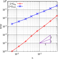
(a)

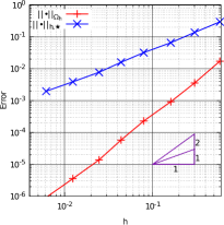
(b)

Figure 1. $H^{1}$ errors and $L^{2}$ errors for the exact solution $u=\sin(x_{1})\sin(x_{2})$.

Subsequently, we consider the exact solution $u(x_{1},x_{2})=((x_{1}+1)^{2}+x_{2}^{2})^{\frac{2}{3}}$ and the corresponding $f$, $g$, and $u_{0}$. Let $\varepsilon=1$. In this case, $u\in H^{2}(\Omega)$ and $u\not\in W^{3,q}(\Omega)$ for any $q>n$. That is, the assumption of Theorem 2 does not satisfied. Figure 2 reports the $H^{1}$ error and the $L^{2}$ error for $\varepsilon=1$. We see from Figure 2 that the convergence rate for the $H^{1}$ error is $O(h)$. However, the second-order convergence does not achieve for the $L^{2}$ error. Actually, we observe that the convergence rate for the $L^{2}$ error is $O(h^{2-\sigma})$ with some small $\sigma>0$. This result is consistent with Theorem 2. Therefore, we can conclude that the regularity condition $u\in W^{3,q}(\Omega)$ with $q>n$ is an essential requirement for deducing the optimal order convergence.

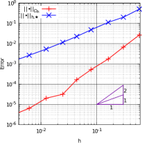
Figure 2. $H^{1}$ errors and $L^{2}$ errors for the exact solution $u=((x_{1}+1)^{2}+x_{2}^{2})^{\frac{2}{3}}$

Acknowledgements

This work was supported by CREST (JPMJCR15D1) of JST, Japan, by Grant-in-Aid for Scientific Research B (15H03635) of JSPS, Japan, and by Grant-in-Aid for Scientific Research A (21H04431) of JSPS, Japan.

References

[1]
R. A. Adams and John J. F. Fournier.
Sobolev spaces, volume 140 of Pure and Applied Mathematics
(Amsterdam).
Elsevier/Academic Press, Amsterdam, second edition, 2003.
[2]
I. Babuška.
The theory of small changes in the domain of existence in the theory
of partial differential equations and its applications.
In Differential Equations and Their Applications (Proc.
Conf., Prague, 1962), pages 13–26. Publ. House Czechoslovak Acad. Sci.,
Prague; Academic Press, New York, 1963.
[3]
I. Babuška.
The finite element method with penalty.
Math. Comp., 27:221–228, 1973.
[4]
J. W. Barrett and C. M. Elliott.
Finite element approximation of the Dirichlet problem using the
boundary penalty method.
Numer. Math., 49(4):343–366, 1986.
[5]
J. W. Barrett and C. M. Elliott.
Finite-element approximation of elliptic equations with a Neumann
or Robin condition on a curved boundary.
IMA J. Numer. Anal., 8(3):321–342, 1988.
[6]
Y. Bazilevs and T. J. R. Hughes.
Weak imposition of Dirichlet boundary conditions in fluid
mechanics.
Comput. & Fluids, 36(1):12–26, 2007.
[7]
Y. Bazilevs, C. Michler, V. M. Calo, and T. J. R. Hughes.
Weak Dirichlet boundary conditions for wall-bounded turbulent
flows.
Comput. Methods Appl. Mech. Engrg., 196(49-52):4853–4862,
2007.
[8]
L. Cherfils, M. Petcu, and M. Pierre.
A numerical analysis of the Cahn-Hilliard equation with dynamic
boundary conditions.
Discrete Contin. Dyn. Syst., 27(4):1511–1533, 2010.
[9]
P. G. Ciarlet.
The Finite Element Method for Elliptic Problems.
North-Holland Publishing Co., Amsterdam-New York-Oxford, 1978.
[10]
C. A. Figueroa, I. E. Vignon-Clementel, K. E. Jansen, T. J. R. Hughes, and
C. A. Taylor.
A coupled momentum method for modeling blood flow in
three-dimensional deformable arteries.
Comput. Methods Appl. Mech. Engrg., 195(41-43):5685–5706,
2006.
[11]
M. Juntunen and R. Stenberg.
Nitsche’s method for general boundary conditions.
Math. Comp., 78(267):1353–1374, 2009.
[12]
T Kashiwabara, C. M. Colciago, L. Dedè, and A. Quarteroni.
Well-posedness, regularity, and convergence analysis of the finite
element approximation of a generalized Robin boundary value problem.
SIAM J. Numer. Anal., 53(1):105–126, 2015.
[13]
T. Kashiwabara and T. Kemmochi.
Pointwise error estimates of linear finite element method for
Neumann boundary value problems in a smooth domain.
Numer. Math., 144(3):553–584, 2020.
[14]
T. Kashiwabara, I. Oikawa, and G. Zhou.
Penalty method with P1/P1 finite element approximation for the
Stokes equations under the slip boundary condition.
Numer. Math., 134(4):705–740, 2016.
[15]
J. T. King.
New error bounds for the penalty method and extrapolation.
Numer. Math., 23:153–165, 1974.
[16]
J. Nitsche.
Über ein Variationsprinzip zur Lösung von
Dirichlet-Problemen bei Verwendung von Teilr äumen, die keinen
Randbedingungen unterworfen sind.
Abh. Math. Sem. Univ. Hamburg, 36:9–15, 1971.
Collection of articles dedicated to Lothar Collatz on his sixtieth
birthday.
[17]
F. Nobile and C. Vergara.
An effective fluid-structure interaction formulation for vascular
dynamics by generalized Robin conditions.
SIAM J. Sci. Comput., 30(2):731–763, 2008.
[18]
N. Saito.
On the Stokes equation with the leak and slip boundary conditions
of friction type: regularity of solutions.
Publ. Res. Inst. Math. Sci., 40(2):345–383, 2004.