Fast Communication-efficient Spectral Clustering Over Distributed Data

Abstract

The last decades have seen a surge of interests in distributed computing thanks to advances in clustered computing and big data technology. Existing distributed algorithms typically assume all the data are already in one place, and divide the data and conquer on multiple machines. However, it is increasingly often that the data are located at a number of distributed sites, and one wishes to compute over all the data with low communication overhead. For spectral clustering, we propose a novel framework that enables its computation over such distributed data, with “minimal” communications while a major speedup in computation. The loss in accuracy is negligible compared to the non-distributed setting. Our approach allows local parallel computing at where the data are located, thus turns the distributed nature of the data into a blessing; the speedup is most substantial when the data are evenly distributed across sites. Experiments on synthetic and large UC Irvine datasets show almost no loss in accuracy with our approach while about 2x speedup under various settings with two distributed sites. As the transmitted data need not be in their original form, our framework readily addresses the privacy concern for data sharing in distributed computing.

1 Introduction

Spectral clustering [45, 41, 50, 32, 56] refers to a class of clustering algorithms that work on the eigen-decomposition of the Gram matrix formed by the pairwise similarity of data points. It is widely acknowledged as the method of choice for clustering, due to its typically superior empirical performance, its flexibility in capturing a range of geometries such as nonlinearity and non-convexity [41], and its nice theoretical properties [49, 17, 26, 51, 54]. Spectral clustering has been successfully applied to a wide spectrum of applications, including parallel processing [47], image segmentation [45, 23], robotics [42, 9], web search [10], spam detection, social network mining [52, 40, 34], and market research [11] etc.

Most existing spectral clustering algorithms are “local” algorithms. That is, they assume all the data are in one place. Then either all computation are carried out on a single machine, or the data are split and delegated to a number of nodes (a.k.a. machines or sites) for parallel computation [14, 30]. It is possible that the data may be initially stored at several distributed nodes but then pushed to a central server which split and re-distribute the data. Such a case is also treated as local, as all the data are in one place at a certain stage of the data processing. However, with the emergence of big data, it is increasingly often that the data of interest are distributed. That is, the data are stored at a number of distributed sites, as a result of diverse data collection channels or business operation etc. For example, a major retail vendor, such as Walmart, has sales data collected at walmart.com, or its Walmart stores, or its warehouse chains—Sam’s Club etc. Such data from different sources are distributed as they are owned by different business groups, even all within the same corporation. Indeed there is no one central data center at Walmart, rather the data are either housed at Walmart’s Arkansas headquarter, or its e-commerce labs in the San Francisco Bay area, CA, due possibly to historical reason—Walmart was a pioneer of commercial vendors for a large scale adoption of digital technology in the late seventies to early eighties, while started its e-commerce business during the last decade. Many applications, however, would require data mining or learning of a global nature, that is, to use data from all the distributed sites, as that would be a more faithful representation of the real world or would yield better results due to a larger data size.

There are several challenges in the spectral clustering of data across distributed sites. The data at individual sites may be large. Many existing divide-and-conquer type of algorithms [14, 30] would collect data from distributed sites first, re-distribute the working load and then aggregate results computed at individual sites. The communication overhead will be high. Moreover, the data at individual sites may not have the same distribution. Additionally, the owners of the data at individual sites may not be willing to share either because the data entails value or the data itself may be too sensitive to share (not the focus of this work though). Now the question becomes, can we carry out spectral clustering for data distributed over a number of sites without transmitting large amount data?

One possible solution is to carry out spectral clustering at individual sites and then ensemble. However, as the data distribution at individual sites may be very different, and to ensemble needs distributional information from individual sites which is often not easy to derive. Thus, an ensemble type of algorithm will not work, or, at least not in a straightforward way. Another possibility is to modify existing distributed algorithms, such as [14, 30], but that would require support from the computing infrastructure—to enable a close coordination and frequent communication of intermediate results among individual nodes—which is not easy to implement and the solution may not be generally applicable.

Our proposed framework is based on the distortion minimizing local (DML) transformations [56]. The idea is to generate a small set of codewords (a.k.a. representative points) that preserve the underlying structure of the data at individual nodes. Such codewords are then transmitted to a central server (or any one of the nodes) where spectral clustering is carried out, and the result from spectral clustering will be populated to individual nodes so that the cluster membership of all points can be recovered according to correspondence information maintained at individual nodes. As the codewords from individual sites preserve the geometry of the data, the expected loss in clustering accuracy w.r.t. that where all the data are in one place would be small. The key benefit of our approach lies in the fact that the generation of codewords is local in the sense that no distributional information from other sites is required. Additionally, computation of the codewords can be carried out in parallel on individual nodes thus speeds up the overall computation and meanwhile makes the best use of the existing computing resources.

Our contributions are as follows. Motivated by emerging applications in distributed computing, we propose a new line of research—spectral clustering when the data are distributed over multiple sites. The DML-based framework we propose readily facilitates data mining tasks such as spectral clustering over distributed data while eliminating the need of big data transmission. Our approach is theoretically sound; the loss in the accuracy of spectral clustering, when compared to that in a non-distributed setting, vanishes when increasing the size of data transmission. Major computations are naturally localized and parallelized in the sense that they are carried out on the node where the data is stored, which would lead to a major speedup in the overall computation. Additionally, as each node is working on part of the full data, this has the potential benefit of divide-and-conquer in the sense that even if we add up the computation time at all individual nodes, the total time may still be less than that in a non-distributed setting for big enough data. While this work deals with spectral clustering for concreteness and for being an important methodology at its own right, really it represents a new paradigm in distributed computing, that is, data mining or inference over distributed data with major computation carried out at where the data are located while achieving the effect of using the full data at a “minimal” communication cost.

The remaining of this paper is organized as follows. In Section 2, we will describe our framework and explain its implementation. This is followed by a discussion of related work in Section 3. In Section 4, we present theoretical analysis of our proposed approach. In Section 5, we show experimental results. Finally we conclude in Section 6.

2 A framework for spectral clustering on distributed data

The idea underlying our approach is the notion of continuity. That is, similar data would play a similar role in learning and inference, including clustering. Such a notion suggests a class of data transformations called distortion minimizing local (DML) transformation. The idea of DML transformation is to represent the data by a small set of representative points (or codewords). One can think of this as a “small-loss” data compression, or the representative set as a sketch of the full data. Since the representative set resembles the full data, learning based on it is expected to be close to that on the full data. Similar idea was explored in [56, 5] and has been successfully applied to some computation-intensive algorithms, assuming the data are non-distribted. In all these previous work, DMLs were mainly introduced to address the computational challenge.

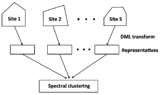
Figure 1: Architecture of spectral clustering over distributed data. Data at different nodes may be of different distributions.

DMLs can be used to enable spectral clustering over distributed data, that is, the data are not stored in one machine but over a number of distributed nodes. Our framework for spectral clustering over distributed data is surprisingly simple to implement. It consists of three steps:

• Apply DML to data at each distributed node

• Collect codewords from all nodes, and carry out spectral clustering on the set of all codewords

• Populate the learned clustering membership by spectral clustering back to each distributed node.

Figure 1 is an illustration of our framework. It is clear that algorithms designed under this framework would eliminate the need of having to transmit large amount of data among distributed nodes—only those codewords need to be transmitted. As the codewords are DML-transformed data, data privacy may be ensured since no original data are transmitted. Additionally, as spectral clustering is only performed on the set of codewords, the overall computation involved will be greatly reduced. Also as the DMLs and the recovering of cluster membership are performed at individual nodes, such computation can be done in parallel. We start by a brief introduction to spectral clustering.

2.1 Introduction to spectral clustering

Spectral clustering works on an affinity graph over data points $X_{1},...,X_{N}$ and seeks to find a “minimal” graph cut. Depending on the choice of the similarity metric and the objective function to optimize, there are a number of variants, including [45, 41]. Our discussion will be based on normalized cuts [45].

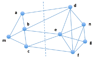
Figure 2: Illustration of a graph cut. The cut is given by the set $\{ad,bd,be,ce,cf\}$, which partitions the vertices of the graph into $V=V_{1}\cup V_{2}=\{a,b,c,m\}\bigcup\{d,e,f,n,g\}$.

An affinity graph is defined as a weighted graph $\mathcal{G}=(V,\mathcal{E},A)$ where $V=\{X_{1},...,X_{N}\}$ is the set of vertices, $\mathcal{E}$ is the edge set, and $A=(a_{ij})_{i,j=1}^{N}$ is the affinity matrix with $a_{ij}$ encoding the similarity between $X_{i}$ and $X_{j}$. Figure 2 is an illustration of graph cut.

Let $V=(V_{1},\ldots,V_{K})$ be a partition of $V$. Define the size of the cut between $V_{1}$ and $V_{2}$ by

$$\mathcal{W}(V_{1},V_{2})=\sum_{i\in V_{1},j\in V_{2}}a_{ij}~{}\mbox{for}~{}V_{1},V_{2}\subseteq V.$$

Normalized cuts seeks to find the minimal (normalized) graph cut, or equivalently, solve an optimization problem

$$\arg\min_{V_{1},...,V_{K}\subseteq V}\sum_{j=1}^{K}\frac{\mathcal{W}(V_{j},V)-\mathcal{W}(V_{j},V_{j})}{\mathcal{W}(V_{j},V)}.$$

The above is an integer programming problem thus intractable, a relaxation to real values leads to an eigenvalue problem for the Laplacian matrix

$$\mathcal{L}_{A}=D^{-\frac{1}{2}}(D-A)D^{-\frac{1}{2}},$$ (1)

where $D=diag(d_{1},...,d_{N})$ is the degree matrix with $d_{i}=\sum_{j=1}^{N}a_{ij},i=1,...,N$. Normalized cuts look for the second smallest eigenvector of $\mathcal{L}_{A}$, and round its components to produce a bipartition of the graph. Similar procedure is applied to each of the bipartitions recursively until reaching the number of predefined clusters.

2.2 Distortion minimizing local transformation

A key property that makes DMLs applicable to distributed data is being local. That is, such a data transformation can be done locally, without having to see the full data. Thus DML can be applied at individual distributed nodes separately. If one can pool together all those codewords, then overall inference or data mining can be easily carried out. Thus, as long as the local data transformations are fine enough, a large class of inference or data mining tools will be able to yield result as good as using the full data.

As we are dealing with big volumes of data, a natural requirement for a DML is its computational efficiency while incurring very “little” loss in information. We will briefly describe two concrete implementations of the DML transformation, one by $K$-means clustering and the other by random projection trees (rpTrees), both proposed in [56].

2.2.1 K-means clustering

$K$-means clustering was developed by S. Lloyd in 1957 [38], and remains one of the simplest yet popular clustering algorithms. The goal of $K$-means clustering is to split data into $K$ partitions (clusters) and assign each point to the “nearest” cluster (mean). A cluster mean is the center of mass of all points in a cluster; it is also called cluster centroid or codewords. The algorithm starts with a set of randomly selected cluster centers, then alternates between two steps: 1) assign all points to their nearest cluster centers; 2) recalculate the new cluster centers. The algorithm stops when the change is small according to a cluster quality measure. For a more details about K-means clustering, please refer to the appendix and [29, 38].

When DML is implemented by $K$-means clustering, each of the distributed nodes performs $K$-means clustering separately. Note that, the number of clusters, $K$, may be different for a different node; the only requirement is that $K$ is reasonably large. The set of representative points are taken as the cluster centers, or average of points in the same cluter by an appropriate metric. Empirically, the computation of $K$-means clustering scales linearly with the number of data points, thus it is suitable for big data.

2.2.2 Random projection trees

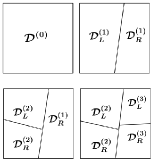
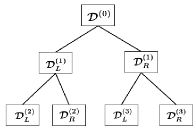
Figure 3: Illustration of space partition and random projection trees (figure taken from [57]). The superscripts indicate the order of tree node split. One starts with the root node, $\mathcal{D}^{(0)}$, which corresponds to all the data. After the first split, $\mathcal{D}^{(0)}$ is partitioned into its two child nodes, $\{\mathcal{D}_{L}^{(1)},\mathcal{D}_{R}^{(1)}\}$. The second split partitions the left child node, $\mathcal{D}_{L}^{(1)}$, into its two child nodes, $\{\mathcal{D}_{L}^{(2)},\mathcal{D}_{R}^{(2)}\}$. The third cut splits $\mathcal{D}_{R}^{(1)}$ into two new child nodes, $\{\mathcal{D}_{L}^{(3)},\mathcal{D}_{R}^{(3)}\}$. This process continues until a stopping criterion is met.

To see how the K-D tree [8] can be used for a DML transformation, we first describe how a K-D tree grows. Let the collection of all data at a distributed site correspond to the root node, $\mathcal{D}^{(0)}$, of a tree. Now one variable, say $v$ (index of a variable), is selected to split the root node; the root node is split into two child nodes, $\mathcal{D}_{L}^{(1)}$ and $\mathcal{D}_{R}^{(1)}$, according to whether a data points has its $v$-th coordinate smaller or larger than a cutoff point. For each of $\mathcal{D}_{L}^{(1)}$ and $\mathcal{D}_{R}^{(1)}$, we will follow a similar procedure recursively. This process continues until some stopping criterion is met. Figure 3 illustrates the construction of a K-D tree. As the tree construction can be viewed as generating a recursive space partition [8, 19, 55] of the data, data points falling in the same leaf node would be similar (if the leaf node is “small”) and their average can be used as the representative. If the underlying data has a very high dimension, then a randomized variant, rpTrees [19], can be used which would adapt to the geometry of the underlying data and effectively overcome the curse of dimensionality. In this work, we use rpTrees implemented in [59].

2.3 Algorithmic description

Now we can briefly describe how to adopt spectral clustering for distributed data. Assume that there are $S$ distributed sites. Apply DML (K-means clustering or rpTrees) at each site individually. Let $Y_{i}^{(s)},i=1,2,...,n_{s}$ be the group centroids of data at site $s=1,2,...,S$. A group is either data in the same cluster if K-means clustering is used, or all points in the same leaf node of rpTrees. The centroids are center of mass of all points in the same group. Spectral clustering is performed on the set of group centroids (representative points) collected from all the $S$ sites. An algorithmic description is given in Algorithm 1.

Algorithm 1   Spectral clustering for distributed data

1:  $\mathcal{D}_{r}\leftarrow\emptyset$;

2:  for each site $s\in\{1,...,S\}$ do

3:     Apply DML to data at site s;

4:     Let $Y_{i}^{(s)},i=1,2,...,n_{s}$ be the group centroids;

5:     Let $W_{i}^{(s)},i=1,2,...,n_{s}$ be the group sizes;

6:     $\mathbb{Y}_{s}\leftarrow\{Y_{i}^{(s)}:i=1,2,...,n_{s}\}$;

7:  end for

8:  Collect group centroids from all sites $\mathcal{D}_{r}\leftarrow\cup_{s=1}^{S}\mathbb{Y}_{s}$;

9:  Spectral clustering on $\mathcal{D}_{r}$;

10:  Populate cluster membership to all $S$ sites;

If the DML transformation is linear, which is the case if it is implemented by K-means clustering or rpTrees, then the overall computational complexity is easily seen to be linear in the total number of points in the distributed data. Indeed for large scale distributed computation, that is an implicit requirement.

3 Related work

There has been an explosive growth of interests in distributed computing in the last decades. One driving force behind is the prevalence of low-cost clustered computers and storage systems [2, 24], which makes it feasible to interconnect hundreds or thousands of clustered computers. Numerous systems and computing platforms have been developed for distributed computing. For example, Google’s Bigtable [25, 12], the Apache Hadoop/Map-Reduce [20, 46], the Spark system [62, 61], and Amzon’s AWS cloud etc. The literature is huge, but mostly on distributed system architecture, computing platforms, or data query tools. For a review of recent developments, please see [13, 21] and references therein.

Existing distributed algorithms in the literature are either parallel algorithms, for example, [14], or use a divide-and-conquer strategy which split the data and distribute the workload to a number of nodes [30]. An influential line of work is Bag of Little Bootstrap [33]. This work aims at computing a big data version of Bootstrap [22], a fundamental tool in statistical inference; the idea is to take many very “thin” subsamples, distribute the computing on each subsample to a node and then aggregate results from those individual subsamples. Recently, [7] considered the general distributed estimation and inference in the Divide-and-Conquer paradigm, and obtained optimal partitions for data. Chen and Xie [16] studied penalized regression and model selection consistency when the data is too big to fit into the memory of a single machine by working on a subsample of the data and then aggregating the resulting models. Singh et al [48] designed DiP-SVM, a distribution preserving kernel support vector machine where the first and second order statistics of the data are retained in each of the data partitions, and run spectral clustering on each data partition at an individual nodes with results aggregated. One thing common about these work is that all assume one has the entire data before delegating the workload to individual nodes or pushing the data to temporary storage and then aggregate the individual results; the data are distributed or split mainly for improving computational efficiency or solving the memory shortage problem.

Many works have been proposed to improve the efficiency of spectral clustering. Chen and Cai [15] proposed a landmark-based method for spectral clustering by selecting representative data points as a linear combination of the original data. Zhang and his co-authors [63] proposed an incremental sampling approach, i.e., the landmark points are selected one at a time adaptively based on the existing landmark points. Liu et al. [37] proposed a fast constrained spectral clustering algorithm via landmark-based graph construction and then reduce the data size by random sampling after spectral embedding. Paiva [43] proposed to select a representative subset of the training sample with an information-theoretic strategy. Lin et al [36] designed a scalable co-association cluster ensemble framework using a compressed version of co-association matrix formed by selecting representative points of the original data.

Several recent work aims at reducing the data volume by deep learning. Aledhari et al [1] proposed a deep learning based method to minimize large genomic DNA dataset for transmission through the internet. Banijamali et al [6] integrated the recent deep auto-encoder technique into landmark-based spectral clustering.

4 Analysis of the algorithm

In our distributed framework, each node $s$ individually applies DML to generate codewords $\mathbb{Y}_{s}=\{Y_{i}^{(s)}:i=1,2,...,n_{s}\}$, to be sent to a central node for spectral clustering. The results from spectral clustering are returned to node $s$ for the recovery of cluster membership for all points at node $s=1,...,S$. A crucial question is, does this approach work? Since each site performs DML locally and no site is using distributional information from others. How much additional error will be incurred under our framework, or will such an error vanish if the data is big? The goal of our analysis is to shed lights to these questions.

To carry out such an analysis is challenging. We are interested in the clustering error (an end-to-end error), but we only observe errors in terms of the local distortion in representing the points, $\mathbb{X}_{s}=\{X_{i}^{(s)}:i=1,2,...,N_{s}\}$ by codeword $\mathbb{Y}_{s}$ for each $s=1,...,S$. We need to establish a connection between the clustering error and the distortion in data representation of a distributed (local) nature.

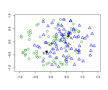
Figure 4: Illustration when the support of data from two different sites overlaps. Data with the same color indicate the same distributed node. The original codewords computed at each node are $A_{1}$ and $A_{2}$ (marker by circle and triangle, respectively), while the optimal codewords (assuming there are two) for the combined data are $B_{1}$ and $B_{2}$ (marked by stars).

A second challenge is related to the local ‘optimality’ of our algorithm. That is, each set of codewords $\mathbb{Y}_{s}$ is an ‘optimal’ representation of data, $\mathbb{X}_{s}$, at a local site, but their union, $\mathbb{Y}=\cup_{s=1}^{S}\mathbb{Y}_{s}$, is not necessary the optimal set of codewords for the entire set of data $\mathbb{X}=\cup_{s=1}^{S}\mathbb{X}_{s}$. One situation for which this happens is when there is an overlap among the support of points from different sites. As illustrated in Figure 4, the original codes $A_{1},A_{2}$ are no longer the optimal codewords for the combined data; rather the new optimal codewords become $B_{1}$ and $B_{2}$. Now the question is, will local ‘optimality’ at all individual sites be sufficient or if additionally constraints may be required to make our approach work?

One crucial insight to our analysis is, what we really need is the convergence of the global distortion to zero when the size of data increases, not necessary the optimality of the global distortion. So we would proceed as if all the data are from one node, and only plugs in analysis of local DMLs when necessary. Our analysis hinges on an important result obtained in [56] which establishes the connection between the end-to-end error and the perturbations to the Laplacian matrix due to data distortion.

Lemma 1 ([56]).

Under assumptions $\mathbb{A}_{1-3}$, the mis-clustering rate $\rho$ of a spectral bi-partitioning algorithm on perturbed data satisfies

$$\rho\leq\|\bm{\tilde{v}}_{2}-\bm{v}_{2}\|^{2}\leq||\tilde{\mathcal{L}}-\mathcal{L}||_{F}^{2},$$

where $||.||_{F}$ indicates the Frobenius norm [27].

By Lemma 1, in order to bound the additional clustering error resulting from the distributed nature of the data, we just need to bound the distortion of the Laplacian matrix due to a compressed data representation by codewords from a number of distributed sites.

We will proceed in two steps. First, we conduct a perturbation analysis of the Laplacian matrix. Then, we will adopt results from local DMLs to the perturbation results. Note that in the perturbation analysis, we treat all the data as if they are all from one site. We follow notations in [56].

Our theoretical model is the following two-component Gaussian mixture

$$G=(1-\pi)\cdot G_{1}+\pi\cdot G_{2},$$ (2)

where $\pi\in\{0,1\}$ with $\mathbb{P}(\pi=1)=\eta$. The choice of a two-component Gaussian mixture is mainly for simplicity; it should be clear that our analysis applies to any finite Gaussian mixtures. We treat data perturbation as adding a noise component $\epsilon$ to $X$:

$$\tilde{X}=X+\epsilon,$$ (3)

and we denote the distribution of $\tilde{X}$ by $\tilde{G}$. We assume $\epsilon$ is symmetric about $0$ with bounded support, and let $\epsilon$ has a standard deviation $\sigma_{\epsilon}$ that is small compared to $\sigma$, the standard deviation for the distribution of $X$.

4.1 Perturbation analysis

Our perturbation analysis relies on one more result established in [56] which is stated as Lemma 2.

Lemma 2 ([56]).

Let $\mathcal{L}$ and $\tilde{\mathcal{L}}$ be the Laplacian matrix corresponding to the original similarity matrix and that after perturbation. Then

$$||\tilde{\mathcal{L}}-\mathcal{L}||_{F}\leq||D^{-\frac{1}{2}}ED^{-\frac{1}{2}}||_{F}\\ +(1+o(1))||\Delta D^{-\frac{3}{2}}AD^{-\frac{1}{2}}||_{F}.$$ (4)

We state without proof some elementary results.

Lemma 3.

Let $a,b\in\mathbb{R}$. Then the following holds

$$(a-b)^{2}\leq 2(a^{2}+b^{2}),~{}(a-b)^{4}\leq 8(a^{4}+b^{4}).$$

The main result of our perturbation analysis is stated as Theorem 1.

Theorem 1.

Suppose $X_{1},...,X_{N}\in\mathbb{R}^{d}$ are generated i.i.d. according to (2) such that $\inf_{1\leq i\leq N}d_{i}/N>\delta_{0}$ holds in probability for some constant $\delta_{0}>0$. Further, the number of data points, $N_{s}$, at site $s$ carries a substantial fraction of the total number of data points $N$ in the sense that $\lim_{N\rightarrow\infty}N_{s}/N=\gamma_{s}\in(0,1)$ for $s=1,...,S$. Assume the data perturbation $\epsilon$ is symmetric about $0$ with bounded support. Further assume $||\Delta D^{-1}||_{2}=o(1)$. Then

$$||\tilde{\mathcal{L}}-\mathcal{L}||_{F}^{2}\leq_{p}C\sum_{s=1}^{S}\gamma_{s}\sigma_{s}^{2}+C^{\prime}\sum_{s=1}^{S}\gamma_{s}\sigma_{s}^{4}$$

for some constants $C$ and $C^{\prime}$, as $N\rightarrow\infty$.

Proof.

Our proof essentially follows that of Theorem 5 and Theorem 6 in [56] except during the final steps of Lemma 13 and Lemma 14. Instead of using theory of U-statistics [31] which would give a sharper bound, we use an upper bound, i.e., Lemma 3, which allows us to group the perturbation error of individual data points by the distributed site they belong to. By adopting the proof of Lemma 13, we have

$$||D^{-\frac{1}{2}}ED^{-\frac{1}{2}}||_{F}^{2}$$

$$\leq \frac{2C}{\delta_{0}^{2}N^{2}}\sum_{i=1}^{N}\sum_{j=1}^{N}(\epsilon_{i}-\epsilon_{j})^{2}+\frac{2}{\delta_{0}^{2}N^{2}}\sum_{i=1}^{N}\sum_{j=1}^{N}R_{max}^{2}(\epsilon_{i}-\epsilon_{j})^{4}$$

$$\leq \frac{4C}{\delta_{0}^{2}N^{2}}\sum_{i=1}^{N}\sum_{j=1}^{N}(\epsilon_{i}^{2}+\epsilon_{j}^{2})+\frac{16}{\delta_{0}^{2}N^{2}}\sum_{i=1}^{N}\sum_{j=1}^{N}R_{max}^{2}(\epsilon_{i}^{4}+\epsilon_{j}^{4})$$

$$= \frac{8C}{\delta_{0}^{2}N}\sum_{i=1}^{N}\epsilon_{i}^{2}++\frac{32}{\delta_{0}^{2}N}\sum_{i=1}^{N}R_{max}^{2}\epsilon_{i}^{4}$$

$$\overrightarrow{a.s.} C_{1}\sum_{s=1}^{S}\gamma_{s}\sigma_{s}^{2}+C_{2}\sum_{s=1}^{S}\gamma_{s}\sigma_{s}^{4}$$

as $N\rightarrow\infty$. In the above $\epsilon_{i}$ is the perturbation to observation $X_{i}$ for $i=1,...,N$. Similarly in the proof of Lemma 14, we have

$$||\Delta D^{-\frac{3}{2}}AD^{-\frac{1}{2}}||_{F}^{2}$$

$$\leq \frac{2}{\delta_{0}^{4}N^{2}}\sum_{i=1}^{N}\sum_{k=1}^{N}\left[C(\epsilon_{i}-\epsilon_{k})^{2}+R_{max}^{2}(\epsilon_{i}-\epsilon_{k})^{4}\right]$$

$$\overrightarrow{a.s.} C_{3}\sum_{s=1}^{S}\gamma_{s}\sigma_{s}^{2}+C_{4}\sum_{s=1}^{S}\gamma_{s}\sigma_{s}^{4}$$

as $N\rightarrow\infty$. Combining the above two inequalities and then apply Lemma 2, we have proved the theorem. ∎

4.2 Quantization errors by K-means clustering

Existing work from vector quantization [60, 28] allows us to characterize the amount of distortion when the representative set is computed by $K$-means clustering.

Let a quantizer $q$ be defined as $q:\mathbb{R}^{d}\mapsto\{y_{1},\ldots,y_{n}\}$ for $y_{i}\in\mathbb{R}^{d}$. For $X$ generated from a random source in $\mathbb{R}^{d}$, let the distortion of $q$ be defined as: $\mathcal{D}(q)=\mathbb{E}||X-q(X)||^{s}$, which is the mean square error for $s=2$. Let $R(q)=\log_{2}n$ denote the rate of the quantization code. Define the distortion-rate function $\delta(R)$ as

$$\delta(R)=\inf_{q:~{}R(q)\leq R}\mathcal{D}(q).$$

Then $\delta(R)$ can be characterized in terms of the source density $f(\cdot)$, and constants $d,s$ by the following theorem.

Theorem 2 ([60, 28]).

Let $f(x)$ be the $d$-dimensional probability density. Then, for large rates $R$, the distortion-rate function of fixed-rate quantization can be characterized as:

$$\delta_{d}(R)\cong b_{s,d}\cdot||f||_{d/(d+s)}\cdot n^{-s/d},$$

where $\cong$ means the ratio of the two quantities tends to 1, $b_{s,d}$ is a constant depending on $s$ and $d$, and

$$||f||_{d/(d+s)}=\left(\int f^{d/(d+s)}(x)dx\right)^{(d+s)/d}.$$

Now we can apply Theorem 2 and Pollard’s strong consistency of K-means clustering [44] to individual terms in Theorem 1, and establish a performance bound for our approach.

Theorem 3.

Assume the data distributions in a S-site distributed environment have density $f_{1},...,f_{S}$, respectively. Let $k_{1},...,k_{S}$ be the number of codewords at the $S$ distributed sites. Let $k=min(k_{1},...,k_{S})$. Then the additional clustering error rate $\rho$, as compared to non-distributed setting, under our framework can be bounded by

$$C\cdot\max_{s=1,...,S}||f_{s}||_{d/(d+2)}.k^{-2/d}+O(k^{-4/d}),$$

where $C$ is a constant determined by the number of clusters, the variance of the original data, the bandwidth of the Gaussian kernel and the eigengap of Laplacian matrix (or minimal eigengap of the Laplacian of all affinity matrices used in normalized cuts).

5 Experiments

In this section, we report our experimental results. This includes simulation results on synthetic data, and on data from the UC Irvine Machine Learning Repository [35]. We will compare the performance of distributed vs non-distributed (where all the data are assumed to be in one place). The spectral clustering algorithm used is normalized cuts [45], and the Gaussian kernel is used in computing the affinity (or Gram) matrix with the bandwidth chosen via a cross-validatory search in the range (0, 200] (with step size 0.01 within (0,1], and 0.1 over (1,200]) for each data set. All algorithms are implemented in R programming language, and the kmeans() function in R is used for which details are similar as those documented in [56].

The metric for clustering performance is clustering accuracy, which counts the fraction of labels given by a clustering algorithm that agree with the true labels (or labels come with the dataset). Let $\{1,...,K\}$ denote the set of class labels, and $h(.)$ and $\hat{h}(.)$ are the true label and the label given by the clustering algorithm, respectively. The clustering accuracy is defined as [56]

$$\max_{\tau\in\Pi}\left\{\frac{1}{N}\sum_{i=1}^{N}\mathbb{I}\{\tau(h(x_{i}))=\hat{h}(x_{i})\}\right\},$$ (5)

where $\mathbb{I}$ is the indicator function and $\Pi$ is the set of all permutations on the class labels $\{1,...,K\}$. While there are dozens of performance metrics around for clustering, the clustering accuracy is a good choice for the evaluation of clustering algorithms. This is because the label (or cluster membership) of individual data points is the ultimate goal of clustering, while other clustering metrics are often a surrogate of the cluster membership, and they are used in practice mainly due to the lack of labels. For the evaluation of clustering algorithms, we do have the freedom of using those datasets coming with a label. Indeed the clustering accuracy is commonly used for the evaluation of clustering; see, for example, [53, 4, 56].

We also consider the time for computation. The elapsed time is used. It is counted from the moment when the data are loaded into the memory (R running time environment), till the time when we have obtained the cluster label for all data points. We assume all the distributed nodes run independently, so the longest computation time among all the sites is used (instead of adding them up). As we do not have multiple computers for the experiments, we do not explore the communication time for transmitting representative points and the clustering results. Indeed, for the dataset used in our experiments, such time could be ignored when compared to the computation time, as the number of representative points are all less than 2000. The time reported in this work are produced on a MacBook Air laptop computer, with 1.7GHz Intel Core i7 processor and 8G memory.

5.1 Synthetic data

To appreciate how those representative points look like, we first consider a toy example.

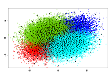
Figure 5: A 4-component Gaussian mixture. Different clusters are indicated by colors. The triangle spots are representative points. Site 1 corresponds to red and blue colors, and Site 2 green and cyan.

The data is generated by a 4-component Gaussian mixture $\frac{1}{4}\sum_{i=1}^{4}\mathcal{N}(\mu_{i},\Sigma)$ with $\mu_{1}=(2,2)$, $\mu_{2}=(-2,-2)$, $\mu_{3}=(-2,2)$ and $\mu_{4}=(2,-2)$, and the covariance matrix given by

$$\Sigma=\begin{bmatrix}3&1\\ 1&3\end{bmatrix}.$$

The Gaussian mixture is commonly used as a generating model for clusters in the literature [18, 39, 51, 58, 54], due to its simplicity (as the mixture components are Gaussians) and also because it is amenable for theoretical analysis. Indeed, it is used as the theoretical model in our analysis (c.f. Section 4). Note that here we are not arguing that spectral clustering is superior to other clustering methods, rather our claim was spectral clustering could work in a distributed setting that we consider.

Figure 5 is a scatter plot of the Gaussian mixture. The four mixture components are marked by blue, red, green, and cyan, respectively. Here in generating representative points, we run $K$-means clustering on the two sites defined by $\mathcal{N}(\mu_{1},\Sigma)+\mathcal{N}(\mu_{2},\Sigma)$ and $\mathcal{N}(\mu_{3},\Sigma)+\mathcal{N}(\mu_{4},\Sigma)$, respectively. It can be seen that those representative points serve as a “good” condensed representation of the original data points.

We conduct experiments on a 4-component Gaussian mixture on $\mathbb{R}^{10}$

$$\frac{1}{4}\sum_{i=1}^{4}\mathcal{N}(\mu_{i},\Sigma)$$ (6)

with the center of the four components being

$$\mu_{1}=(2.5,0,...,0),~{}\mu_{2}=(0,2.5,0,...,0),$$

$$\mu_{3}=(0,0,2.5,0,...,0),~{}\mu_{4}=(0,0,0,2.5,0,...,0),$$

and the covariance matrix $\Sigma$ defined by

$$\Sigma_{i,j}=\rho^{|i-j|},~{}~{}\mbox{for}~{}\rho=0.1,0.3,0.6.$$

For simplicity, we only consider the case with two sites in a distributed environment. It should be easy to extend to the general case. Let $\mathcal{C}_{i},i=1,2,3,4$, denote the data from the four mixture components, respectively. To simulate how the data may look like in a distributed environment, we create the following three scenarios:

• Site 1 has $\mathcal{C}_{1}+\mathcal{C}_{2}$, Site 2 has those from $\mathcal{C}_{3}+\mathcal{C}_{4}$

• Site 1 has $\frac{1}{2}\mathcal{C}_{1}+\mathcal{C}_{2}+\frac{1}{2}\mathcal{C}_{3}$, Site 2 has $\frac{1}{2}\mathcal{C}_{1}+\frac{1}{2}\mathcal{C}_{3}+\mathcal{C}_{4}$

• Site 1 and 2 each has a randomly selected half of the data points

where $\frac{1}{2}\mathcal{C}_{1}$ means that a distributed site contains half of the data points from component $\mathcal{C}_{1}$, and so on. Note these scenarios are not the different ways that we split and distribute the data for fast computation rather each should be viewed as one type of distributed settings: $D_{1}$ for which data at different sites have roughly disjoint supports, $D_{2}$ for which data at different sites have some overlap in terms of supports, and in $D_{3}$ individual sites have similar data distribution. 40000 data points are generated from the Gaussian mixture (6), and the number of representative points is $1000$ (i.e., the data compression ratio is 40:1). The number of data points at Site 1 and 2, and also the number of representative points can all be calculated by the site specification and the data compression ratio accordingly. Note that here the number of clusters in K-means clustering (or the number of leaf nodes in rpTrees) is no longer as important as that in usual clustering, as long as the resulting groups are sufficiently fine (i.e., data points in the same group are “similar”); since here K-means clustering (or rpTrees) is used to group the data for efficient distributed computation. The same discussion applies to UC Irvine datasets as well.

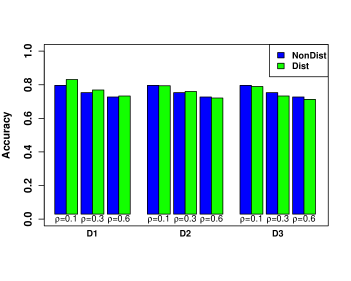
Figure 6: Clustering accuracy by spectral clustering on a 4-component Gaussian mixture with different $\rho$’s when K-means clustering is used as DML. $D_{1},D_{2}$ and $D_{3}$ are 3 simulation scenarios, and there are two distributed sites in all simulations.

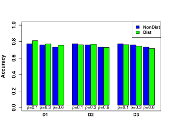
Figure 7: Clustering accuracy by spectral clustering on a 4-component Gaussian mixture with different $\rho$’s when rpTrees is used as DML. $D_{1},D_{2}$ and $D_{3}$ are 3 simulation scenarios, and there are two distributed sites in all simulations.

Figure 6 and Figure 7 show the clustering accuracy of spectral clustering under various distributed scenarios as compared to non-distributed when K-means clustering and rpTrees are used as DML, respectively. Here the true label of each data point is taken as its mixture component ID. The data compression ratio for K-means clustering is set to be 40:1, which is the ratio of the size of the data to the number of clusters in DML; the maximum size of the leaf nodes is 40 for rpTrees, to match approximately the data compression ratio in K-means clustering. In all cases, the accuracy computed for distributed data is close to non-distributed. The reason that the accuracy under $D_{1}$ may be higher than others (including the non-distributed) may be attributed to the fact the data are less mixed than in other settings thus implicitly achieving a regularization effect where data are grouped within the same classes or the part of data that are less mixed than others (one can roughly view this as additional constraints on clustering).

Data set	# Features	# instances	# classes
Connect-4	42	67,557	3
SkinSeg	3	245,057	2
USCI	37	285,779	2
Cover Type	54	568,772	5
HT Sensor	11	928,991	3
Poker Hand	10	1,000,000	3
Gas Sensor	18	8,386,765	2
HEPMASS	28	10,500,000	2

Table 1: A summary of UC Irvine data used in the experiments.

5.2 UC Irvine data

Data set	$\bm{D_{1}}$		$\bm{D_{2}}$		$\bm{D_{3}}$
USCI	$\mathcal{C}_{1}$	$\mathcal{C}_{2}$	0.7$\mathcal{C}_{1}$+0.3$\mathcal{C}_{2}$	0.3$\mathcal{C}_{1}$+0.7$\mathcal{C}_{2}$	50%	50%
SkinSeg
Gas Sensor
HEPMASS
Connect-4	$\mathcal{C}_{1}$	$\mathcal{C}_{2}$+$\mathcal{C}_{3}$	0.5$\mathcal{C}_{1}$+$\mathcal{C}_{2}$	0.5$\mathcal{C}_{1}$+$\mathcal{C}_{3}$	50%	50%
HT Sensor
Poker Hand
Cover type	$\mathcal{C}_{2}$	$\mathcal{C}_{1}$+$\mathcal{C}_{3-5}$	0.7$\mathcal{C}_{1}$+0.3$\mathcal{C}_{2}$	0.3$\mathcal{C}_{1}$+0.7$\mathcal{C}_{2}$	50%	50%
			+$\mathcal{C}_{3-5}$

Table 2: A summary of simulation settings. Here $D_{1},D_{2},D_{3}$ are 3 distributed simulation scenarios considered in this work.

The UC Irvine datasets we use include the Connect-4, SkinSeg (Skin segmentation), USCI (US Census Income), Cover type, HT Sensor, Poker Hand, Gas Sensor and the HEPMASS data. Table 1 gives a summary of the datasets. For Connect-4, USCI, and Poker Hand data, we follow procedures described in [56] to preprocess the data. The original USCI data has 299,285 instances with 41 features. We excluded instances with missing values, and also features #26, #27, #28 and #30, due to too many values. This leaves 285,799 instances on $37$ features, with all categorical variables converted to integers. The original Cover Type data has 581,012 instances. We excluded the two small classes (i.e., 4 and 5) for fast evaluation of accuracy (otherwise all 7! permutations need to be evaluated, but that is not our focus of the feasibility of distributed computing), and this leaves 568,772 instances; we also standardized the first 10 features such that each has a mean 0 and variance 1. The original Poker Hand data is highly unbalanced, with $6$ small classes containing less than $1\%$ of the data. Merging small classes gives $3$ final classes with a class distribution of $50.12\%$, $42.25\%$ and $7.63\%$, respectively. The Gas Sensor data consists of two different gas mixtures: Ethylene mixed with CO, and Ethylene mixed with Methane. The data corresponding to these two gas mixtures form the two classes in the data. The Connect-4, the USCI, and the Gas Sensor data are normalized such that all features have mean $0$ and standard deviation $1$.

It is worthwhile to remark that, though the datasets we use may be smaller than some large data at industry-scale, the Gas Sensor and the HEPMASS are among the largest datasets currently available in the UC Irvine data repository. Moreover, in industry often the raw data used may be huge but, after preprocessing and feature engineering, the data used for data mining or model building are substantially smaller. Additionally, the UC Irvine datasets used in our experiments have a wide variety of sizes, ranging from 67,557 to 10,500,000. We believe those are sufficient to demonstrate the feasibility of our algorithm for distributed computing; for even larger data, results from our theoretical analysis (large sample asymptotics) can be used to gain insights.

Similar as the synthetic data, we conduct experiments under three distributed settings for each UC Irvine dataset. Table 2 lists the site specification under such settings. These settings are all common in practice. $D_{1}$ corresponds to situations where different sites have data with disjoint supports, and $D_{2}$ the case where data from different sites are mixed in terms of the support of the data, while $D_{3}$ is for the case where the data at each site is a random sample from a common data distribution. Each of $D_{1}$, $D_{2}$ and $D_{3}$ in Table 2 corresponds to two columns with the left indicating the data composition for Site 1 and the right for Site 2 (under $D_{3}$ each of the two distributed sites has a random half of the full data). The number of data points at Site 1 and 2, and also the number of representative points can all be calculated by the site specification and the data compression ratio accordingly.

Data set	Non-distributed	$\bm{D_{1}}$	$\bm{D_{2}}$	$\bm{D_{3}}$
Connect-4	0.6569	0.6576	0.6569	0.6569
	36	17	15	12
SkinSeg	0.9482	0.9516	0.9406	0.9425
	18	13	9	8
USCI	0.9356	0.9382	0.9404	0.9396
	215	199	104	63
Cover type	0.4984	0.4987	0.4979	0.4986
	402	221	207	264
HT Sensor	0.4960	0.5008	0.4972	0.4978
	55	23	16	23
Poker Hand	0.4977	0.4993	0.4982	0.5006
	123	67	65	62
Gas Sensor	0.9865	0.9887	0.9866	0.9846
	620	287	258	254
HEPMASS	0.7929	0.7949	0.7927	0.7902
	8752	3275	3263	3321

Table 3: Clustering accuracy and running time on UC Irvine data under 3 simulation settings, $D_{1},D_{2}$ and $D_{3}$, when K-means clustering is used as the DML. The time is in seconds. There are two distributed sites under all of $D_{1},D_{2}$ and $D_{3}$.

Table 3 show the clustering accuracy and elapsed time for each UC Irvine dataset under settings $D_{1},D_{2}$, and $D_{3}$, respectively, when K-means clustering is used as DML. The data compression ratios are 200, 800, 500, 500, 3000, 3000, 16000 and 7000, respectively. Table 4 is for rpTrees. Due to the random nature of rpTrees, it is hard to set the exact data compression ratio. To match the compression ratio for K-means clustering, we set the maximum size of leaf nodes to be 200, 800, 500, 500, 3000, 3000, 16000 and 7000, respectively. It can be seen that, for all cases, the loss in clustering accuracy due to distributed computing is small. By local computation at individual distributed sites in parallel, the overall time required for spectral clustering is significantly reduced. When the computation is evenly distributed across different sites, the saving in time is often most substantial; this is typically the case under $D_{3}$ where data are evenly split among two sites. At the similar level of data compression, DML by rpTrees is more efficient in computation than that by K-means clustering, but incurs slightly more loss in accuracy. Note that for simplicity, we consider two distributed sites for all the UC Irvine data except the HEPMASS data. For the rest of this section, we explore 3 or 4 distributed sites for the HEPMASS data.

Data set	Non-distributed	$\bm{D_{1}}$	$\bm{D_{2}}$	$\bm{D_{3}}$
Connect-4	0.6577	0.6560	0.6554	0.6550
	7	6	5	5
SkinSeg	0.9492	0.9535	0.9434	0.9432
	5	4	3	3
USCI	0.9394	0.9391	0.9394	0.9371
	36	33	23	19
Cover type	0.4978	0.4984	0.4956	0.4968
	81	50	52	53
HT Sensor	0.4957	0.4963	0.4893	0.4836
	26	10	7	7
Poker Hand	0.4990	0.4999	0.4976	0.4993
	47	26	25	24
Gas Sensor	0.9828	0.9850	0.9811	0.9792
	305	174	175	169
HEPMASS	0.7906	0.7920	0.7902	0.7890
	1568	695	688	712

Table 4: Clustering accuracy and running time on UC Irvine data under 3 simulation settings, $D_{1},D_{2}$ and $D_{3}$, when rpTrees is used as the DML. The time is in seconds. There are two distributed sites under all of $D_{1},D_{2}$ and $D_{3}$.

5.2.1 Multiple sites

To study the impact of the number of distributed sites to our algorithm, we run our algorithm on the HEPMASS data for 3 or 4 distributed sites. The site configuration is shown in Table 5 where, for completeness, we also include the case of two sites from the previous section. The results are shown in Table 6. We can see that in all cases, the clustering accuracy does not or degrade very little when increasing of the number of distributed sites. For both cases, i.e., with K-means or rpTrees as the DML, the running time decreases when more sites are involved. However, the decreasing trend gradually slows down; such a phenomenon is more pronounced for the case of rpTrees as the local computation takes much less time than by K-means. This is because, as more distributed sites are involved, eventually most of the computation time would be on spectral clustering part.

# Sites	Settings	Site configuration
2	$D_{1}$	Site1: $C_{1}$,  Site2: $C_{2}$
	$D_{2}$	Site1: $0.7C_{1}+0.3C_{2}$,  Site2: $0.3C_{1}+0.7C_{2}$
	$D_{3}$	Data randomly partitioned among sites
3	$D_{1}$	Site1: $C_{1}/2$,  Site2: $C_{1}/2$,  Site3: $C_{2}$
	$D_{2}$	Site1: $C_{1}/2+C_{2}/4$,  Site2: $C_{1}/4+C_{2}/4$,
		Site3: $C_{1}/4+C_{2}/2$
	$D_{3}$	Data randomly partitioned among sites
4	$D_{1}$	Site1: $C_{1}/2$,  Site2: $C_{1}/2$,  Site3: $C_{2}/2$,
		Site4: $C_{2}/2$
	$D_{2}$	Site1: $3/8C_{1}+C_{2}/8$,  Site2: $3/8C1+C_{2}/8$,
		Site3: $C_{1}/8+3/8C_{2}$,  Site4: $C_{1}/8+3/8C_{2}$
	$D_{3}$	Data randomly partitioned among sites

Table 5: Simulation setting for HEPMASS data with multiple distributed sites.

Non-distributed	DML	$\bm{D_{1}}$	$\bm{D_{2}}$	$\bm{D_{3}}$
	kmeans2	0.7949	0.7927	0.7902
		3275	3263	3321
0.7929	kmeans3	0.7937	0.7913	0.7904
8752		3159	2469	2106
	kmeans4	0.7905	0.7887	0.7891
		1474	1413	1465
	rptrees2	0.7920	0.7902	0.7890
		695	688	712
0.7906	rptrees3	0.7895	0.7900	0.7866
1568		678	564	526
	rptrees4	0.7876	0.7884	0.7869
		387	396	401

Table 6: Clustering accuracy and running time (in seconds) on the HEPMASS data under settings, $D_{1},D_{2}$ and $D_{3}$, respectively. The subscripts next to the DML are the number of distributed sites.

6 Conclusion

We have proposed a novel framework that enables spectral clustering for distributed data, with “minimal” communication overhead while a major speedup in computation. Our approach is statistically sound in the sense that the achieved accuracy is as good as that when all the data are in one place. Our approach achieves computational speedup by deeply compressing the data with DMLs (which also sharply reduce the amount of data transmission) and leveraging existing computing resources for local parallel computing at individual nodes. The speedup in computation, compared to that in a non-distributed setting, is expected to scale linearly (with a potential of even faster when the data is large enough) with the number of distributed nodes when the data are evenly distributed across individual sites. Indeed, on all large UC Irvine datasets used in our experiments, our approach achieves a speedup of about 2x when there are two distributed sites. Two concrete implementations of DMLs are explored, including that by K-means clustering and by rpTrees. Both can be computed efficiently, i.e., computation (nearly) linear in the number of data points. One additional feature of our framework is that, as the transmitted data are not in their original form, data privacy may also be preserved.

Our proposed framework is promising as a general tool for data mining over distributed data. Methods developed under our framework will allow practitioners to use potentially much larger data than previously possible, or to attack problems previously not feasible, due to the lack of data for various reasons, such as the challenges in big data transmission and privacy concerns in data sharing.

Appendix

6.1 The K-means clustering algorithm

Formally, given $n$ data points, $K$-means clustering seeks to find a partition of $K$ sets $S_{1},S_{2},...,S_{K}$ such that the within-cluster sum of squares, $SS_{W}$, is minimized

$$\underset{S_{1},S_{2},...,S_{K}}{\operatorname{arg\,min}}\sum_{i=1}^{K}\sum_{\mathbf{x}\in S_{i}}\left\|\mathbf{x}-\bm{\mu}_{i}\right\|^{2},$$ (7)

where $\mu_{i}$ is the centroid of $S_{i},i=1,2,...,K$.

Directly solving the problem formulated as (7) is hard, as it is an integer programming problem. Indeed it is a NP-hard problem [3]. The K-means clustering algorithm is often referred to a popular implementation sketched as Algorithm 2 below. For more details, one can refer to [29, 38].

Algorithm 2 $K$-means clustering algorithm

1:  Generate an initial set of $K$ centroids $m_{1},m_{2},...,m_{K}$;

2:  Alternate between the following two steps

3:      Assign each point $x$ to the “closest” cluster

$$\arg\min_{j\in\{1,2,...,K\}}\big{\|}x-m_{j}\big{\|}^{2};$$

4:      Calculate the new cluster centroids

$$m_{j}^{new}=\frac{1}{\|S_{j}\|}\sum_{x\in S_{j}}x,~{}~{}j=1,2,...,K;$$

5:  Stop when cluster assignment no longer changes.

6.2 The random projection tree algorithm

in this section, we given an algorithmic description of the generation of rpTrees which we adopt from [59]. Let $U$ denote the given data set. Let $t$ denote the rpTree to be built from $U$. Let $\mathcal{W}$ denote the set of working nodes. Let $n_{T}$ denote a predefined constant for the minimal number of data points in a tree node for which we will split further. Let $P_{\stackrel{{\scriptstyle\rightharpoonup}}{{r}}}(x)$ denote the projection coefficient of point $x$ onto line $\stackrel{{\scriptstyle\rightharpoonup}}{{r}}$. Let $\mathcal{N}$ denote the set of neighborhoods, and each element of $\mathcal{N}$ is a subset of neighboring points in $U$.

Algorithm 3   rpTree(U)

1:  Let $U$ be the root node of tree $t$;

2:  Initialize the set of working nodes $\mathcal{W}\leftarrow\{U\}$;

3:  while $\mathcal{W}$ is not empty do

4:     Randomly pick $W\in\mathcal{W}$ and set $\mathcal{W}\leftarrow\mathcal{W}-\{W\}$;

5:     if $|W|<n_{T}$ then

6:        Skip to the next round of the while loop;

7:     end if

8:     Generate a random direction $\stackrel{{\scriptstyle\rightharpoonup}}{{r}}$;

9:     Project points in $W$ onto $\stackrel{{\scriptstyle\rightharpoonup}}{{r}}$, and let $W_{\stackrel{{\scriptstyle\rightharpoonup}}{{r}}}=\{r\bm{\cdot}x:x\in W\}$;

10:     Let $a=\min(W_{\stackrel{{\scriptstyle\rightharpoonup}}{{r}}})$ and $b=\max(W_{\stackrel{{\scriptstyle\rightharpoonup}}{{r}}})$;

11:     Generate a splitting point $c\sim runif[a,b]$;

12:     Split node $W$ by $W_{L}=\{x:P_{\stackrel{{\scriptstyle\rightharpoonup}}{{r}}}(x)<c\}$ and $W_{R}=\{x:P_{\stackrel{{\scriptstyle\rightharpoonup}}{{r}}}(x)\geq c\}$;

13:     Update working set by $\mathcal{W}\leftarrow\mathcal{W}\cup\{W_{L},W_{R}\}$;

14:  end while

15:  return(t);

References

- [1] M. Aledhari, M. D. Pierro, M. Hefeida, and F. Saeed. A Deep Learning-Based Data Minimization Algorithm for Fast and Secure Transfer of Big Genomic Datasets. IEEE Transactions on Big Data, PP:1–13, 2018, doi: 10.1109/TBDATA.2018.2805687.
- [2] A. C. Arpaci-Dusseau, R. H. Arpaci-Dusseau, D. E. Culler, J. M. Hellerstein, and D. A. Patterson. High-performance sorting on networks of workstations. In ACM SIGMOD International Conference on Management of Data, May 1997.
- [3] D. Arthur and S. Vassilvitskii. How slow is the K-means method? In Proceedings of the Symposium on Computational Geometry, 2006.
- [4] F. R. Bach and M. I. Jordan. Learning spectral clustering, with application to speech separation. Journal of Machine Learning Research, 7:1963–2001, 2006.
- [5] M. Badoiu, S. Har-Peled, and P. Indyk. Approximate clustering via core-sets. In Fortieth ACM Symposium on Theory of Computing (STOC), 2002.
- [6] E. Banijamali and A. Ghodsi. Fast spectral clustering using autoencoders and landmarks. In 14th International Conference on Image Analysis and Recognition, pp. 380–388, 2017.
- [7] H. Battey, J. Fan, H. Liu, J. Lu, and Z. Zhu. Distributed testing and estimation under sparse high dimensional models. The Annals of Statistics, 46(3):1352–1382, 2018.
- [8] J. Bentley. Multidimensional binary search trees used for associative searching. Communications of the ACM, 18(9):509–517, 1975.
- [9] E. Brunskill, T. Kollar, and N. Roy. Topological mapping using spectral clustering and classification. In Proceedings of the IEEE International Conference on Intelligent Robots and Systems, pp. 3491–3496, October 2007.
- [10] D. Cai, X. He, Z. Li, W. Ma, and J. Wen. Hierarchical clustering of www image search results using visual, textual and link information. In Proceedings of the 12th Annual ACM International Conference on Multimedia, pp. 952–959, 2004.
- [11] E.-C. Chang, S.-C. Huang, H.-H. Wu, and C.-F. Lo. A case study of applying spectral clustering technique in the value analysis of an outfitter’s customer database. In Proceedings of the IEEE International Conference on Industrial Engineering and Engineering Management, 2007.
- [12] F. Chang, J. Dean, S. Ghemawat, W. C. Hsieh, D. A. Wallach, M. Burrows, T. Chandra, A. Fikes, and R. E. Gruber. Bigtable: A Distributed Storage System for Structured Data. In Seventh Symposium on Operating System Design and Implementation (OSDI), November 2006.
- [13] M. Chen, S. Mao, and Y. Liu. Big data: A survey. Mobile Networks and Applications, 19:171–209, 2014.
- [14] W.-Y. Chen, Y. Song, H. Bai, C.-J. Lin, and E. Y. Chang. Parallel spectral clustering in distributed systems. IEEE Transactions on Pattern Analyses and Machine Intelligence, 33(3):568–586, 2011.
- [15] X. Chen and D. Cai. Large scale spectral clustering with landmark-based representation. In AAAI, 2011.
- [16] X. Chen and M. Xie. A split-and-conquer approach for analysis of extraordinarily large data. Statistica Sinica, 24:1655–1684, 2014.
- [17] F. Chung. Spectral Graph Theory. American Mathematical Society, 1997.
- [18] S. Dasgupta. Learning mixtures of Gaussians. In Proceedings of the 40th Annual Symposium on Foundations of Computer Science (FOCS), 1999.
- [19] S. Dasgupta and Y. Freund. Random projection trees and low dimensional manifolds. In Fortieth ACM Symposium on Theory of Computing (STOC), 2008.
- [20] J. Dean and S. Ghemawat. MapReduce: Simplified Data Processing on Large Clusters . In Sixth Symposium on Operating System Design and Implementation (OSDI), December 2004.
- [21] S. Dolev, P. Florissi, E. Gudes, S. Sharma, and I. Singer. A Survey on Geographically Distributed Big-Data Processing using MapReduce. IEEE Transactions on Big Data, 3:79–90, 2017.
- [22] B. Efron. Bootstrap methods: another look at the Jacknife. Annals of Statistics, 7(1):1–28, 1979.
- [23] C. Fowlkes, S. Belongie, F. Chung, and J. Malik. Spectral grouping using the Nystrm method. IEEE Transactions on Pattern Analysis and Machine Intelligence, 26(2):214–225, 2004.
- [24] A. Fox, S. D. Gribble, Y. Chawathe, E. A. Brewer, and P. Gauthier. Cluster-based scalable network services. In 16th ACM Symposium on Operating Systems Principles, pp. 78–91, 1997.
- [25] S. Ghemawat, H. Gobioff, and S.-T. Leung. The Google file system. In 19th ACM Symposium on Operating Systems Principles, pp. 29–43, 2003.
- [26] E. Giné and V. Koltchinskii. Empirical graph Laplacian approximation of Laplace-Beltrami operators: Large sample results. In High Dimensional Probability: Proceedings of the Fourth International Conference, 2006.
- [27] G. H. Golub and C. F. Van Loan. Matrix Computations. Johns Hopkins, 1989.
- [28] R. M. Gray and D. L. Neuhoff. Quantization. IEEE Transactions of Information Theory, 44(6):2325–2383, October, 1998.
- [29] J. A. Hartigan and M. A. Wong. A K-means clustering algorithm. Applied Statistics, 28(1):100–108, 1979.
- [30] M. Hefeeda, F. Gao, and W. Abd-Almageed. Distributed approximate spectral clustering for large-scale datasets. In Proceedings of the 21st International Symposium on High-Performance Parallel and Distributed Computing (HPDC), pp. 223–234, 2012.
- [31] W. Hoeffding. The strong law of large numbers for U-statistics. Technical Report 302, University North Carolina Institute of Statistics Mimeo Series, 1961.
- [32] L. Huang, D. Yan, M. I. Jordan, and N. Taft. Spectral clustering with perturbed data. In Advances in Neural Information Processing Systems (NIPS), volume 21, pp. 705–712, 2009.
- [33] A. Kleiner, A. Talwalkar, P. Sarkar, and M. I. Jordan. A scalable bootstrap for massive data. Journal of the Royal Statistical Society: Series B (Statistical Methodology), 76(4):795–816, 2014.
- [34] M. Kurucz, A. Bencz r, K. Csalog ny, and L. Luk cs. Spectral clustering in social networks. In Advances in Web Mining and Web Usage Analysis, pp. 1–20, 2009.
- [35] M. Lichman. UC Irvine Machine Learning Repository. http://archive.ics.uci.edu/ml, 2013.
- [36] Z. Lin, F. Yang, Y. Lai, X. Gao, and T. Wang. A scalable approach of co-association cluster ensemble using representative points. 32nd Youth Academic Annual Conference of Chinese Association of Automation (YAC), pp. 1194–1199, 2017.
- [37] W. Liu, M. Ye, J. Wei, and X. Hu. Fast constrained spectral clustering and cluster ensemble with random projection. In Computational Intelligence and Neuroscience, 2017.
- [38] S. P. Lloyd. Least squares quantization in PCM. IEEE Transactions on Information Theory, 28(1):128–137, 1982.
- [39] G. J. McLachlan and D. Peel. Finite Mixture Models. Wiley, 2000.
- [40] G. Miao, Y. Q. Song, D. Zhang, and H. J. Bai. Parallel spectral clustering algorithm for large-scale community data mining. In The 17th International World Wide Web Conference (WWW), 2008. Available at http://citeseerx.ist.psu.edu/viewdoc/summary?doi=10.1.1.592.4118.
- [41] A. Y. Ng, M. I. Jordan, and Y. Weiss. On spectral clustering: analysis and an algorithm. In Neural Information Processing Systems (NIPS), volume 14, 2002.
- [42] E. Olson, M. Walter, S. Teller, and J. Leonard. Single-Cluster Spectral Graph Partitioning for Robotics Applications. In Proceedings of Robotics: Science and Systems, pp. 265–272, 2005.
- [43] António R. C. Paiva. Information-theoretic dataset selection for fast kernel learning. 2017 International Joint Conference on Neural Networks (IJCNN), pp. 2088–2095, 2017.
- [44] D. Pollard. Strong consistency of K-means clustering. The Annals of Statistics, 9(1):135–140, 1981.
- [45] J. Shi and J. Malik. Normalized cuts and image segmentation. IEEE Transactions on Pattern Analysis and Machine Intelligence, 22(8):888–905, 2000.
- [46] K. Shvachko, H. Kuang, S. Radia, and R. Chansler. The Hadoop Distributed File System. In IEEE 26th Symposium on Mass Storage Systems and Technologies (MSST), pp. 1–10, May 2010.
- [47] H. D. Simon. Partitioning of unstructured problems for parallel processing. Computing Systems in Engineering, 2:135–148, 1991.
- [48] D. Singh, D. Roy, and C. K. Mohan. DiP-SVM: Distribution Preserving Kernel Support Vector Machine for Big Data. IEEE Transactions on Big Data, 3:79–90, 2017.
- [49] D. A. Spielman and S.-H. Teng. Spectral partitioning works: Planar graphs and finite element meshes. In IEEE Symposium on Foundations of Computer Science, pp. 96–105, 1996.
- [50] U. von Luxburg. A tutorial on spectral clustering. Statistics and Computing, 17(4):395–416, 2007.
- [51] U. von Luxburg, M. Belkin, and O. Bousquet. Consistency of spectral clustering. Annals of Statistics, 36(2):555–586, 2008.
- [52] S. White and P. Smyth. A spectral clustering approach to finding communities in graphs. In Proceedings of IEEE International Conference on Data Mining (ICDM), pp. 76–84, 2005.
- [53] E. Xing, A. Y. Ng, M. I. Jordan, and S. Russell. Distance metric learning, with application to clustering with side-information. In Proceedings of Neural Information Processing Systems (NIPS), pp. 521–528, 2002.
- [54] D. Yan, A. Chen, and M. I. Jordan. Cluster Forests. Computational Statistics and Data Analysis, 66:178–192, 2013.
- [55] D. Yan and G. E. Davis. The turtleback diagram for conditional probability. The Open Journal of Statistics, 8(4):684–705, 2018.
- [56] D. Yan, L. Huang, and M. I. Jordan. Fast approximate spectral clustering. Technical Report 772, Department of Statistics, UC Berkeley, 2009.
- [57] D. Yan, T. W. Randolph, J. Zou, and P. Gong. Incorporating Deep Features in the Analysis of Tissue Microarray Images. Statistics and Its Interface, 12(2):283–293, 2019.
- [58] D. Yan, P. Wang, B. S. Knudsen, M. Linden, and T. W. Randolph. Statistical methods for tissue microarray images–algorithmic scoring and co-training. The Annals of Applied Statistics, 6(3):1280–1305, 2012.
- [59] D. Yan, Y. Wang, J. Wang, H. Wang, and Z. Li. K-nearest neighbor search by random projection forests. In Proceedings of the IEEE International Conference on Big Data, pp. 4775–4781, 2018.
- [60] P. L. Zador. Asymptotic quantization error of continuous signals and the quantization dimension. IEEE Transactions of Information Theory, 28:139–148, 1982.
- [61] M. Zaharia, M. Chowdhury, T. Das, A. Dave, J. Ma, M. McCauley, M. J. Franklin, S. Shenker, and I. Stoica. Resilient Distributed Datasets: A Fault-tolerant Abstraction for In-memory Cluster Computing. In Proceedings of the 9th USENIX Conference on Networked Systems Design and Implementation (NSDI), 2012.
- [62] M. Zaharia, M. Chowdhury, M. J. Franklin, S. Shenker, and I. Stoica. Spark: Cluster Computing with Working Sets. In Proceedings of the 2nd USENIX Conference on Hot Topics in Cloud Computing, 2010.
- [63] X. Zhang, L. Zong, Q. You, and X. Yong. Sampling for Nyström extension-based spectral clustering: Incremental perspective and novel analysis. ACM Transactions on Knowledge Discovery from Data (TKDD), 11:7:1–7:25, 2016.