Exceptional points for resonant states on parallel circular dielectric cylinders

Abstract

Exceptional points (EPs) are special parameter values of a non-Hermitian eigenvalue problem where eigenfunctions corresponding to a multiple eigenvalue coalesce. In optics, EPs are associated with a number of counter-intuitive wave phenomena, and have potential applications in lasing, sensing, mode conversion and spontaneous emission processes. For open photonic structures, resonant states are complex-frequency solutions of the Maxwell’s equations with outgoing radiation conditions. For open dielectric structures without material gain or loss, the eigenvalue problem for resonant states can have EPs, since it is non-Hermitian due to radiation losses. For applications in nanophotonics, it is important to understand EPs for resonant states on small finite dielectric structures consisting of conventional dielectric materials. To achieve this objective, we study EPs of resonant states on finite sets of parallel infinitely-long circular dielectric cylinders with subwavelength radii. For systems with two, three and four cylinders, we develop an efficient numerical method for computing EPs, present examples for second and third order EPs, and highlight their topological features. Our work provides insight to understanding EPs on more complicated photonic structures, and can be used as a simple platform to explore applications of EPs.

1 Introduction

One of the most interesting features of non-Hermitian eigenvalue problems is the existence of exceptional points (EPs), where two or more eigenvalues, as well as their corresponding eigenfunctions, coalesce [1, 2, 3, 4, 5, 6]. For optical systems, EPs exist in eigenvalue problems directly formulated from Maxwell’s equations or indirectly formulated from scattering operators, and the non-Hermiticity comes from material loss and/or gain, or radiation loss for open structures. Associated with EPs, many interesting wave phenomena have been theoretically studied and experimentally observed [6]. These unique features have found valuable applications in unidirectional propagation [7], lasing [8, 9, 10, 11], sensing [12, 13, 14, 15, 16], mode conversion [17], and spontaneous emission processes [18]. Many works on EPs and their applications are associated with parity-time (${\cal PT}$) symmetric optical systems with a balanced gain and loss [19, 20, 21, 22]. In that case, EPs can be easily found by tuning a single parameter, namely, the amplitude of the balanced gain and loss. Since it is not always easy or desirable to keep a balanced gain and loss in an optical system, it is of significant interest to explore EPs and their applications in non-${\cal PT}$-symmetric optical systems. EPs can appear in open dielectric systems with a real dielectric function [23, 24, 25, 26, 27], since power can radiate to infinity in open systems, and the eigenvalue problem for resonant states, directly formulated from Maxwell’s equations with an outgoing radiation condition, is non-Hermitian. Currently, there exist a few studies concerning EPs for resonant states on periodic dielectric structures sandwiched between two homogeneous half-spaces [23, 24, 25, 26]. For these structures, EPs are relatively easy to obtain due to the additional degrees of freedom associated with Bloch wavenumbers, they are related to Dirac points in the band structures of two-dimensional photonic crystals [23], and can be traced to some special points in the band structures of uniform slabs [25]. In addition, paired EPs on periodic dielectric structures exhibit interesting topological properties [26]. For non-periodic dielectric structures, EPs can be found by tuning two or more geometric or material parameters. A multilayered concentric dielectric cylinder is probably the simplest structure on which EPs of resonant modes have been found [27].

For applications in nanophotonics, it is important to have EPs on structures with a size on the optical wavelength. In addition, it is also important to realize EPs without tuning the dielectric constant, since available dielectric materials are limited in practice. In this paper, we analyze EPs for a small number of parallel and infinitely-long dielectric cylinders. The structures are chosen for their simplicity. Our objective is to gain insight about EPs on small non-periodic structures consisting of conventional dielectric materials. We are interested in EPs of resonant states with relatively high quality factors and relatively low resonant frequencies, so that the radii of the cylinders and the distances between them are smaller than or about the same as the resonant wavelength. For systems with two, three and four cylinders, we develop an efficient numerical method for computing EPs and determine second and third order EPs where two or three eigenpairs coalesce.

The rest of this paper is organized as follows. In section 2, we briefly describe the method for computing resonant modes and show an example where resonant modes exhibit crossing and anti-crossing behavior with respect to their dependence on a system parameter. In section 3, we present a method for computing EPs, show second order EPs for systems with two or more cylinders, and discuss their topological features. Third order EPs and related topological properties are studied in section 4. The paper is concluded with a brief discussions in section 5.

2 Resonant modes

For structures that are invariant along the $z$ axis and the $E$-polarization, the $z$ component of the electric field, denoted as $u$, satisfies the following Helmholtz equation

$$\frac{\partial^{2}u}{\partial x^{2}}+\frac{\partial^{2}u}{\partial y^{2}}+k^{2}\varepsilon(x,y)u=0,$$ (1)

where $\varepsilon=\varepsilon(x,y)$ is the dielectric function, $k=\omega/c$ is the free-space wavenumber, $\omega$ is the angular frequency, and $c$ is the speed of light in vacuum. The time dependence is assumed to be $\exp(-i\omega t)$. For the $H$-polarization, the $z$ component of the magnetic field, also denoted as $u$, satisfies the following slightly different Helmholtz equation

$$\frac{\partial}{\partial x}\left(\frac{1}{\varepsilon(x,y)}\frac{\partial u}{\partial x}\right)+\frac{\partial}{\partial y}\left(\frac{1}{\varepsilon(x,y)}\frac{\partial u}{\partial y}\right)+k^{2}u=0.$$ (2)

A resonance mode (or resonant state) is a non-zero solution of Eq. (1) or Eq. (2) satisfying an outgoing radiation condition as $r:=\sqrt{x^{2}+y^{2}}\to\infty$. If the structure is finite (in the $xy$-plane) and surrounded by air, then $\varepsilon(x,y)=n_{0}^{2}$ for sufficiently large $r$, $n_{0}\approx 1$ is the refractive index of air, and the wave field of a resonant mode can be expanded as

$$u({\bf r})=\sum_{m=-\infty}^{\infty}\hat{u}_{m}H_{m}^{(1)}(kn_{0}r)e^{im\theta},$$ (3)

for sufficiently large $r$, where ${\bf r}=(x,y)$, $\theta$ is the polar angle, $H_{m}^{(1)}$ is the Hankel function of first kind and order $m$, and $\hat{u}_{m}$ are expansion coefficients. Since each term in the right hand side of (3) radiates power to infinity and there is no source or incoming wave, a resonant mode can only exist for a complex $k$, so that it can decay with time. Under the assumed time dependence, the imaginary part of $k$ must be negative.

If the structure consists of $N$ parallel circular cylinders surrounded by air, where the cylinders have centers ${\bf c}_{j}$, radii $R_{j}$ and dielectric constants $\varepsilon_{j}$ for $1\leq j\leq N$, the classical multipole method [28, 29, 30, 31] is probably the most efficient method for solving Eqs. (1) and (2). Outside the cylinders, the wave field of a resonant mode can be expanded as

$$u({\bf r})=\sum_{j=1}^{N}\sum_{m=-\infty}^{\infty}b_{m}^{(j)}H_{m}^{(1)}(kn_{0}r_{j})e^{im\theta_{j}},$$ (4)

where $r_{j}$ and $\theta_{j}$ are the magnitude and polar angle of ${\bf r}-{\bf c}_{j}$, respectively, and $b_{m}^{(j)}$ are expansion coefficients. The multipole method gives a homogeneous linear system

$$A(k)\,\mathbf{b}=\mathbf{0},$$ (5)

where $\mathbf{b}$ is a column vector for all $b_{m}^{(j)}$ with $m$ truncated to a finite integer set. More details about Eq. (5) are given in Appendix A. Here, we consider Eq. (5) as an eigenvalue problem with $k$ being the eigenvalue. Since matrix $A$ depends on $k$ nonlinearly, it is a nonlinear eigenvalue problem. Notice that both $k$ and ${\bf b}$ are unknown, and ${\bf b}$ has to be a nonzero vector. Since a nonzero ${\bf b}$ is only possible when $A(k)$ is singular, we can determine $k$ from the condition that $A(k)$ is a singular matrix. As in [32], we solve $k$ from $\lambda_{1}(A)=0$, where $\lambda_{1}(A)$ is the linear eigenvalue of $A$ with the smallest magnitude and it is regarded as a function of $k$. Once $k$ is determined, ${\bf b}$ can be calculated as the eigenvector corresponding to the zero linear eigenvalue of $A$, then the wave field outside the cylinders can be evaluated using Eq. (4), and field inside each cylinder can also be evaluated [30]. See Appendix A for more details.

As an example, we consider two cylinders separated by a distance $\delta$ as shown in Fig. 1.

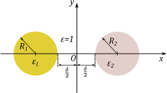
Figure 1: Two circular cylinders parallel to the $z$ axis and surrounded by air.

Assuming the cylinders have dielectric constants $\varepsilon_{1}=\varepsilon_{2}=11.56$ and radii $R_{1}=1$ and $R_{2}=1.66$, we calculate resonant modes of $E$-polarization for a varying spacing $\delta$. For simplicity, we take $R_{1}$ as the characteristic length scale to non-dimensionalize other quantities. For example, $R_{2}$ is regarded as $R_{2}/R_{1}$, $\delta$ is regarded as $\delta/R_{1}$, and $k$ should be interpreted as $kR_{1}$. The complex wavenumbers $k$ for two resonant modes are shown in Fig. 2.

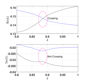
Figure 2: Crossing and anti-crossing in the real and imaginary parts of $k$ (as functions of distance $\delta$) of two resonant modes on a system with two cylinders.

It can be observed that the real parts of $k$ have a crossing at $\delta\approx 0.88$, but the imaginary parts of $k$ avoid the crossing. In fact, the field patterns of the two modes are quite similar at the crossing, yet their decay rates are different due to the anti-crossing in $\mathrm{Im}(k)$. It is also common for the real parts of $k$ to exhibit an anti-crossing and the imaginary parts of $k$ to have a crossing.

3 Second order exceptional points

A second order EP is a non-Hermitian degeneracy where two eigenvalues coincide and their eigenfunctions coalesce. In general, it is necessary to tune two system parameters to find a second order EP. For a set of circular cylinders, the system parameters include geometric and material parameters such as the radii and dielectric constants of the cylinders and the distances between them. Since available dielectric materials are limited, it is desired to find EPs by tuning only the geometric parameters. For the nonlinear eigenvalue problem given in Eq. (5), a second order EP occurs at a complex value of $k$ where the matrix $A$ has a double singularity. One approach is to calculate $k$ from the two conditions $\mathrm{det}(A)=d[\det(A)]/dk=0$ [33]. If the size of matrix $A$ is not very small, it is more robust to use the smallest linear eigenvalue of $A$ instead of its determinant [32]. Therefore, we solve $k$ from the following two conditions

$$\lambda_{1}(A)=\frac{d}{dk}\lambda_{1}(A)=0.$$ (6)

A rigorous justification for the second condition above, i.e., $d\lambda_{1}(A)/dk=0$, is given in Appendix B. Since $\lambda_{1}(A)$ is complex, the two conditions in (6) give rise to a system of four real equations, and it can be used to solve four real unknowns, i.e., the real and imaginary parts of $k$ and two system parameters. We use MATLAB function fsolve to solve the nonlinear system, and it requires a vector function that inputs $\mbox{Re}(k)$, $\mbox{Im}(k)$ and two system parameters, and outputs real and imaginary parts of $\lambda_{1}(A)$ and $d\lambda_{1}(A)/dk$. For a given structure and a given complex $k$, the matrix $A$ can be formed when the infinite sum over $m$ in Eq. (4) is properly truncated, $\lambda_{1}(A)$ can be calculated by MATLAB function eigs, and $d\lambda_{1}(A)/dk$ can be approximated using a difference formula. Initial guesses for $k$ and the two system parameters are needed.

For a single homogeneous circular cylinder, the resonant modes can be solved analytically. The solutions are well-separated and no EPs can be found. In a recent work, Kullig et al. [27] found some EPs for an inhomogeneous cylinder with different but concentric layers. However, their EPs exist at very special values of dielectric constants. For two or more cylinders, more geometric parameters are available, and they can be tuned to find EPs. As a first example, we consider two identical circular and homogeneous cylinders separated by a distance $\delta$ and surrounded by air. Assuming the radius of the two cylinders is $R=1$ (i.e. the radius is used as the characteristic length scale), the system has only two parameters $\delta$ and $\varepsilon$ (the dielectric constant of the cylinders). We obtain a second order EP for the $E$-polarization at $\delta=1.78773$ and $\varepsilon=6.23690$. The complex wavenumber of the resonant mode at this EP is $k=3.72476-0.13420i$, its quality factor is $Q=-0.5\mbox{Re}(k)/\mbox{Im}(k)\approx 13.878$, and the resonant wavelength is $2\pi/\mbox{Re}(k)\approx 1.6869$. Since $R$ is used as the length scale, the above resonant wavelength should be interpreted as its ratio with $R$. The electric field pattern of the resonant mode is shown in Fig. 3.

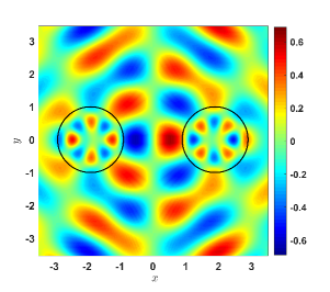
Figure 3: Electric field (real part of $u$) of a resonant mode at an EP on two identical cylinders.

The field patterns inside the cylinders resemble two identical whispering gallery modes with opposite signs. It appears that the coalescence of these two modes gives rise to a rather strong field outside the cylinders. Overall, the electric field is odd in $x$ and even in $y$, where $x$ is the horizontal axis passing through the centers of the two cylinders. For this problem, the two complex conditions in Eq. (6) allow us to determine two real parameters $\delta$ and $\varepsilon$ and the complex wavenumber $k$.

For real applications, it is unlikely that there is a material with the precise dielectric constant at which the EP exists. For this reason, we revert to a system with two circular cylinders with different radii as shown in Fig. 1. We assume the dielectric constants of both cylinders are fixed at $\varepsilon_{1}=\varepsilon_{2}=11.56$, and the radius of one cylinder is $R_{1}=1$. The available geometric parameters are $R_{2}$ and $\delta$. Solving the two complex equations in (6), we obtain a second order EP for the $E$-polarization at $R_{2}=1.66056$ and $\delta=0.88440$. The complex wavenumber of the resonant mode at this EP is $k=4.14671-0.02706i$, and the $Q$-factor is 76.632. The electric field pattern is shown in Fig. 4.

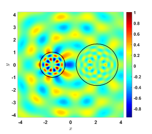
Figure 4: Electric field (real part of $u$) of a resonant mode at a second order EP on two cylinders with $\varepsilon_{1}=\varepsilon_{2}=11.56$, $R_{1}=1$, $R_{2}=1.66056$ and $\delta=0.88440$.

It looks like the field is approximately the superposition of two modes concentrated in the two cylinders. For the $H$-polarization, we found two EPs at $R_{2}=2.30294$ and $\delta=0.22186$, and $R_{2}=2.09224$ and $\delta=0.53607$, respectively. The complex wavenumber and quality factor of the resonant mode at the first EP are $k=1.15695-0.08219i$ and $Q=7.0383$. Those of the resonant mode at the second EP are $k=2.49077-0.08261i$ and $Q=15.075$. The magnetic field patterns of the resonant modes at these two EPs are shown in Fig. 5

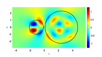
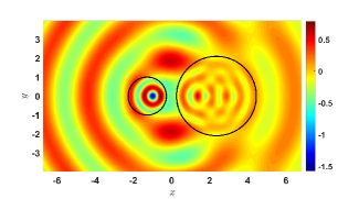
Figure 5: Magnetic field patterns of the resonant modes at two EPs for the $H$-polarization. The upper panel is for the first EP at $R_{2}=2.30294$ and $\delta=0.22186$, and the lower panel is for the second EP at $R_{2}=2.09224$ and $\delta=0.53607$.

It is known that an EP can be verified by its topological signature in the parameter space. Consider the EP for the $E$-polarization above, and let $k_{1}$ and $k_{2}$ be two eigenvalues emerged from the eigenvalue at the EP when the parameters move away from the EP by slightly increasing $\delta$. It is known that encircling an EP in the parameter space (i.e. the $\delta$-$R_{2}$ plane) leads the eigenvalues $k_{1}$ and $k_{2}$ to switch their positions on the associated Riemann surfaces of $\mathrm{Re}(k)$ and $\mathrm{Im}(k)$. In Fig. 6,

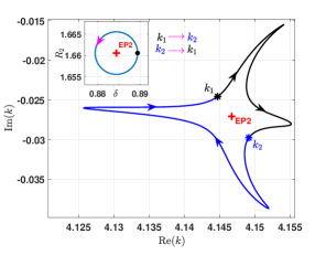
Figure 6: Encircling an EP in the parameter space, $\delta$-$R_{2}$ plane, showing the switching of the eigenvalues $k_{1}\to k_{2}$ and $k_{2}\to k_{1}$.

we show the switching $k_{1}\to k_{2}$ and $k_{2}\to k_{1}$, as $(\delta,R_{2})$ moves alone the circle shown in the inset. The particular parameters that give rise to $k_{1}$ and $k_{2}$ correspond to the dot on the circle. It is well known that a second order EP is a branch point where solutions manifest square-root splittings in both $\mathrm{Re}(k)$ and $\mathrm{Im}(k)$. In Appendix B, we show that this is true even for nonlinear eigenvalue problems. In Fig. 7,

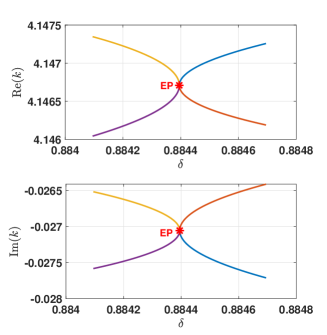
Figure 7: Square-root splitting of the real (top) and imaginary (bottom) parts of $k$ versus $\delta$ near a second order EP.

the real and imaginary parts of $k$ are shown as functions of $\delta$ varying around the EP value 0.88440. The radius $R_{2}$ is fixed at $1.66056$.

The quality factors of the resonant modes at the above EPs are not very high. Since it is desirable to have high $Q$ resonances, we consider a slightly more complicated system with one inhomogeneous cylinder and one homogeneous cylinder as shown in Fig. 8.

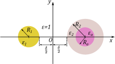
Figure 8: A system of two cylinders of which one has a circular core with radius $R_{a}$ and dielectric constant $\varepsilon_{a}$.

The inhomogeneous cylinder consists of a circular core with radius $R_{a}$ and dielectric constant $\varepsilon_{a}$ and a shell with outer radius $R_{2}$ and dielectric constant $\varepsilon_{2}$. The other parameters $R_{1}$, $\varepsilon_{1}$ and $\delta$ are defined as before. Assuming $\varepsilon_{1}=\varepsilon_{2}=11.56$, $\varepsilon_{a}=10.20$, $R_{1}=1$, and $R_{2}=1.66$, the system has two remaining parameters $\delta$ and $R_{a}$. An EP for the $E$-polarization is found at $\delta=0.734985$ and $R_{a}=0.561180$. The complex wavenumber and quality factor of the resonant mode at this EP is $k=4.16669-0.01824i$ and $Q=114.20$. Its electric field is shown in Fig. 9.

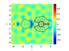
Figure 9: Electric field (real part of $u$) of a resonant mode at an EP on a two-cylinder structure where one cylinder has a core.

The next example consists of four identical cylinders with their centers located at the corners of a rectangle with sides parallel to the $x$ and $y$ axes. Assuming the radius and the dielectric constant of the cylinders are $R=1$ and $\varepsilon_{1}=11.56$, the system still has two free parameters $\delta_{x}$ and $\delta_{y}$, i.e, the horizontal and vertical distance between two cylinders. Using the same method, we obtain two second order EPs for the $E$-polarization. The results are listed in Table 1 below.

EP	(a)	(b)
$\delta_{x}$	0.06453	0.56679
$\delta_{y}$	1.65891	1.03352
$\mbox{Re}(k)$	3.21529	3.58809
$\mbox{Im}(k)$	-0.01081	-0.01517
$Q$-factor	148.73	118.25

Table 1: Second order EPs for a system of four identical cylinders with radius $R=1$, dielectric constant $\varepsilon=11.56$, horizontal distance $\delta_{x}$ and vertical distance $\delta_{y}$.

The electric field patterns of the resonant modes at these two EPs, labeled as (a) and (b), are shown in Fig. 10.

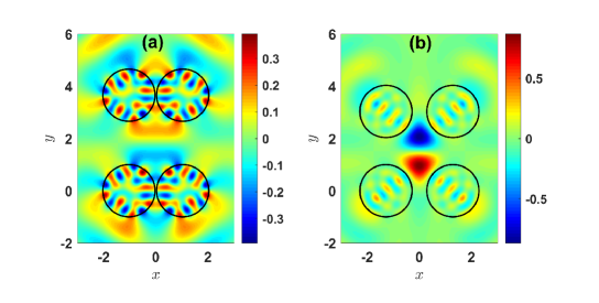
Figure 10: Electric fields (real part of $u$) of resonant modes at two EPs on a system of four parallel identical cylinders.

Exceptional point (a) is obtained when the horizontal distance is very small compared with the radius. Strong electric field appears inside the cylinders. Exceptional point (b) has a strong field at the center of the structure and outside four cylinders. The quality factors of EPs (a) and (b) are $148.73$ and $118.25$, respectively.

For the above examples, the resonant wavelength, given by $(2\pi)/\mbox{Re}(k)$, is close to the diameter of the reference cylinder. The size of the structure in the $xy$ plane is about 3 to 4 wavelengths. Exceptional points at which the resonant modes have higher quality factors can be obtained if one considers higher resonant frequencies (smaller resonant wavelengths) or increases the dielectric constants of the cylinders.

4 Third-order exceptional points

Higher order EPs have extra advantages in some applications [14, 18]. For our problem formulated as Eq. (5), a third order EP occurs only when the matrix $A$ has a triple singularity. As shown in Appendix B, we can find third order EPs by solving the following equations

$$\lambda_{1}(A)=\frac{d}{dk}\lambda_{1}(A)=\frac{d^{2}}{dk^{2}}\lambda_{1}(A)=0.$$ (7)

In general, a third order EP can only be found by tuning four system parameters. The three complex equations above are equivalent to six real equations, and they can only be satisfied if there are six real unknowns. Since the complex $k$ corresponds to two real unknowns, four additional real parameters are needed.

In the following, we present examples of third order EPs in a system with three collinear parallel cylinders as shown in Fig. 11.

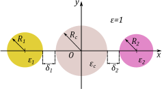
Figure 11: Three parallel dielectric cylinders centered on the $x$-axis.

The centers of the three cylinder are all located on the $x$ axis. The radius and dielectric constant of the cylinder at the center is denoted as $R_{c}$ and $\varepsilon_{c}$, and the distances between the nearby cylinder are $\delta_{1}$ and $\delta_{2}$. We first assume $R_{c}=1$, $\varepsilon_{c}=11.56$, $\delta_{1}=\delta_{2}=0.12$, and consider $R_{1}$, $R_{2}$, $\varepsilon_{1}$ and $\varepsilon_{2}$ as free parameters. Solving Eq. (7) for the $E$-polarization, we obtain a third order EP for $R_{1}=0.95461$, $R_{2}=0.46557$, $\varepsilon_{1}=4.44741$, $\varepsilon_{2}=13.55975$, and $k=4.82031-0.03264i$. The quality factor of the resonant mode at this EP is $Q=73.831$. The field pattern of the resonant mode is shown in Fig. 12.

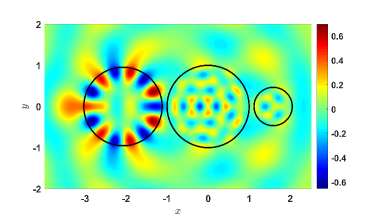
Figure 12: Electric field (real part of $u$) at a third order EP on a system of three cylinders.

A strong field around the first cylinder can be observed, and it resembles a whispering gallery mode of azimuthal order $m=7$.

To verify the EP, we first perturb the system by setting $\delta_{1}=0.125$ away from the EP condition, and keep $R_{1}$, $R_{2}$ and $\delta_{2}$ fixed. Three distinct eigenvalues appear near the complex $k$ of the third order EP, and they are denoted as $k_{A}$, $k_{B}$ and $k_{C}$. As $\delta_{1}$ is continuously decreased to $0.12$, the three eigenvalues coalesce at the EP as shown in Fig. 13.

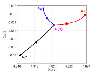
Figure 13: The coalescence of three eigenvalues $k_{A}$, $k_{B}$ and $k_{C}$ as parameter $\delta_{1}$ is decreased from $0.125$ to $0.12$.

Next, we encircle the EP in the parameter space, $\delta_{1}$-$\delta_{2}$ plane, in the counterclockwise direction as shown in the inset of Fig. 14.

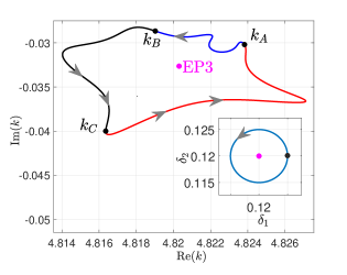
Figure 14: Encircling a third order EP3 in the $\delta_{1}$-$\delta_{2}$ plane. The arrows in the complex $k$ plane follow the arrow in the inset.

The circle in the $\delta_{1}$-$\delta_{2}$ plane includes the point $(\delta_{1},\delta_{2})=(0.125,0.12)$ (the black dot in the inset) that gives rise to $k_{A}$, $k_{B}$ and $k_{C}$. As the parameters $\delta_{1}$ and $\delta_{2}$ move along the circle, the three eigenvalues follow the paths shown in Fig. 14. After one round in the parameter space, the eigenvalues switch as $k_{A}\to k_{B}$,  $k_{B}\to k_{C}$,  and $k_{C}\to k_{A}$. If we encircle the EP in the clockwise direction, then the eigenvalues switch as $k_{A}\to k_{C}$,  $k_{B}\to k_{A}$,  and $k_{C}\to k_{B}$. This is a well-known topological signature of EPs.

For this system of three cylinders, it is also possible to find third order EPs without tuning the dielectric constants $\varepsilon_{1}$, $\varepsilon_{2}$ or $\varepsilon_{c}$. As an example, we let $\varepsilon_{1}=4.45$, $\varepsilon_{2}=13.50$, $\varepsilon_{c}=11.56$ and $R_{c}=1$, and search the four geometric parameters $R_{1}$, $R_{2}$, $\delta_{1}$ and $\delta_{2}$ for third order EPs. One third order EP is found at $R_{1}=0.95426$, $R_{2}=0.46659$, $\delta_{1}=0.11956$ and $\delta_{2}=0.11906$. The complex wavenumber of the resonant mode at this EP is $k=4.82056-0.03269i$. Its field pattern is nearly identical to the one obtained for fixed $\delta_{1}=\delta_{2}=0.12$.

5 Conclusion

Motivated by potential applications in nanophotonics, we analyzed EPs for resonant states on simple structures consisting of a few parallel circular dielectric cylinders surrounded by air. Second and third order EPs are determined for a few structures involving two to four cylinders. They are further validated by analyzing the switching of eigenvalues, a topological signature of the EPs, when pairs of parameters encircle the EPs in parameter spaces. Importantly, EPs can be achieved for structures with given dielectric constants by tuning only the geometric parameters. It is found that the quality factors of the resonant modes at the EPs can be more than 100 when the structure consists of ordinary dielectric materials and the overall size of the structure is restricted to about 3 to 4 wavelengths. Depending on the particular configuration, the wave field of a resonant mode at an EP can be concentrated in or outside the cylinders. For simplicity, we studied only simple two-dimensional structures with infinitely-long and circular cylinders. It is anticipated that if cylinders with more complicated shapes are allowed, the resonant modes at the EPs may have more desirable field distributions. It is known that on carefully designed structures with restrictions on dielectric constants and size as in this paper, some resonant modes unrelated to EPs can have very large quality factors [34]. It is important to find out whether resonant modes at EPs on similar structures can have significantly larger quality factors. For practical applications, the cylinders of finite height must be studied. These studies may benefit from the recently developed vertical mode expansion method (VMEM) for scattering problems involving multiple non-circular cylinders of finite height [35, 36, 37]

Appendix A

For a system with $N$ circular cylinders surrounded by a homogeneous medium of refractive index $n_{0}$, the matrix $A$ in Eq. (5) is an $N\times N$ block matrix, ${\bf b}$ is a vector with $N$ blocks, and they are

$$A=\left[\begin{matrix}I&-S_{1}T_{12}&-S_{1}T_{13}&\cdots\cr-S_{2}T_{21}&I&-S_{2}T_{23}&\cdots\cr-S_{3}T_{31}&-S_{3}T_{32}&I&\cdots\cr\vdots&\vdots&\vdots&\ddots\end{matrix}\right],\quad{\bf b}=\left[\begin{matrix}{\bf b}_{1}\cr{\bf b}_{2}\cr{\bf b}_{3}\cr\vdots\end{matrix}\right],$$

where ${\bf b}_{j}$ is a column vector of $b_{m}^{(j)}$ for all $m$, $S_{j}$ is a diagonal matrix, and $I$ is the identity matrix. Assuming the center, radius and refractive index of the $j$th cylinder are ${\bf c}_{j}$, $R_{j}$ and $n_{j}$, respectively, then the $(m,q)$ entry of matrix $T_{jp}$ is $(T_{jp})_{mq}=H_{m-q}^{(1)}(kn_{0}r_{j}^{p})\exp[i(q-m)\theta_{j}^{p}]$, where $(r_{j}^{p},\theta_{j}^{p})$ are the polar coordinates of ${\bf c}_{p}-{\bf c}_{j}$. For the $E$ polarization, the $(m,m)$ entry of $S_{j}$ is

$$(S_{j})_{mm}=\frac{n_{j}J_{m}(\xi)J^{\prime}_{m}(\eta)-n_{0}J_{m}(\eta)J^{\prime}_{m}(\xi)}{-n_{j}H_{m}^{(1)}(\xi)J^{\prime}_{m}(\eta)+n_{0}J_{m}(\eta){H_{m}^{(1)}}^{\prime}(\xi)},$$

where $\xi=kn_{0}R_{j}$ and $\eta=kn_{j}R_{j}$. For the $H$ polarization, the formula for $(S_{j})_{mm}$ can be obtained by swapping $n_{0}$ and $n_{j}$. If we choose a positive integer $m_{*}$ and truncate $m$ to $-m_{*}\leq m\leq m_{*}$, then ${\bf b}_{l}$ is a vector of length $M=2m_{*}+1$, $T_{jp}$ and $S_{j}$ are $M\times M$ matrices, and $A$ is an $(MN)\times(MN)$ matrix. More details can be found in [30].

Appendix B

To justify Eqs.(6) and (7), we need a perturbation theory about how eigenvalues depend on parameters near an EP for nonlinear eigenvalue problems. For linear eigenvalue problems, this is the well-known power-$1/n$ splitting for $n$-th order EPs [18]. In the following, we clarify the results for second and third order EPs in nonlinear eigenvalue problems.

Consider the following nonlinear eigenvalue problem

$$N(\beta,\lambda)v=0,$$ (8)

where $N$ is a square matrix, $\beta$ is a parameter, $\lambda$ is the eigenvalue, and $v$ is the eigenvector (a non-zero vector). There is also a left eigenvector $w$ such that $w^{T}N(\beta,\lambda)=0$. Clearly, $\lambda$, $v$ and $w$ all depend on $\beta$.

For a second order EP, we have two eigenvalues $\lambda_{j}(\beta)$ ($j=1,2$) and eigenvectors $v_{j}(\beta)$ and $w_{j}(\beta)$ ($j=1,2$), and they satisfy $\lambda_{j}(\beta)\to\lambda_{*}$, $v_{j}(\beta)\to v_{*}$, $w_{j}(\beta)\to w_{*}$ as $\beta\to\beta_{*}$, where $\beta_{*}$ is the parameter value for the EP. For $\beta$ near $\beta_{*}$, we have

$$N(\beta,\lambda_{1})=N(\beta,\lambda_{2})+(\lambda_{1}-\lambda_{2})N^{\prime}(\beta,\lambda_{2})+\frac{1}{2}(\lambda_{1}-\lambda_{2})^{2}N^{\prime\prime}(\beta,\lambda_{2})+...$$

where $N^{\prime}$ and $N^{\prime\prime}$ denote first and second order partial derivatives of $N$ with respect to $\lambda$. Since $w_{1}^{T}N(\beta,\lambda_{1})=0$, we have

$$0=\frac{1}{\lambda_{1}-\lambda_{2}}w_{1}^{T}N(\beta,\lambda_{1})v_{2}=w_{1}^{T}\left[N^{\prime}(\beta,\lambda_{2})+\frac{1}{2}(\lambda_{1}-\lambda_{2})N^{\prime\prime}(\beta,\lambda_{2})+...\right]v_{2}.$$

Taking the limit as $\beta\to\beta_{*}$, we obtain the following self-orthogonality condition

$$w_{*}^{T}N^{\prime}_{*}v_{*}=0,$$ (9)

where $N^{\prime}_{*}=N^{\prime}(\beta_{*},\lambda_{*})$.

In the following, we denote $\lambda_{1}$ and $\lambda_{2}$ simply as $\lambda$, and expand the eigenvalues, eigenvectors and the matrix $N$ in a power series of $\sqrt{\delta}$, where $\delta=\beta-\beta_{*}$. The use of $\sqrt{\delta}$ is necessary, since otherwise the perturbation theory will become inconsistent. We have

$$\lambda(\beta)=\lambda_{*}+C_{1}\sqrt{\delta}+C_{2}\delta+...$$ (10)

$$v(\beta)=v_{*}+v^{(1)}\sqrt{\delta}+v^{(2)}\delta+...$$ (11)

$$w(\beta)=w_{*}+w^{(1)}\sqrt{\delta}+w^{(2)}\delta+...$$ (12)

$$N(\beta,\lambda)=N_{*}+C_{1}N^{\prime}_{*}\sqrt{\delta}+(\partial_{\beta}N_{*}+C_{2}N^{\prime}_{*}+0.5C_{1}^{2}N^{\prime\prime}_{*})\delta+...$$ (13)

where $N_{*}$ denotes $N(\beta_{*},\lambda_{*})$, etc. Inserting the above to $N(\beta,\lambda)v(\beta)=0$, we have $N_{*}v_{*}=0$ at $O(1)$ and $N_{*}v^{(1)}+C_{1}N^{\prime}_{*}v_{*}=0$ at $O(\sqrt{\delta})$. Due to the self-orthogonality, the equation

$$N_{*}y_{1}=-N^{\prime}_{*}v_{*}$$ (14)

has a solution. Thus, $v^{(1)}=C_{1}y_{1}$. At $O(\delta)$, we have

$$N_{*}v^{(2)}+\partial_{\beta}N_{*}v_{*}+C_{2}N^{\prime}_{*}v_{*}+0.5C_{1}^{2}N^{\prime\prime}_{*}v_{*}+C_{1}N^{\prime}_{*}v^{(1)}=0.$$

Multiplying the above by $w_{*}^{T}$, we get

$$C_{1}^{2}=-\frac{w_{*}^{T}\partial_{\beta}N_{*}v_{*}}{w_{*}^{T}(N^{\prime}_{*}y_{1}+0.5N^{\prime\prime}_{*}v_{*})}.$$ (15)

The two solutions of $C_{1}$ (with $\pm$ signs) correspond to the two eigenvalues.

For a third order EP, we have three eigenvalues $\lambda_{j}(\beta)\to\lambda_{*}$, three eigenvectors $v_{j}(\beta)\to v_{*}$, and three left eigenvectors $w_{j}(\beta)\to w_{*}$, as $\beta\to\beta_{*}$ for $j=1$, 2, 3, where $\beta_{*}$ corresponds to the EP. For $\delta=\beta-\beta_{*}$, we assume

$$\lambda(\beta)=\lambda_{*}+C_{1}\delta^{1/3}+C_{2}\delta^{2/3}+C_{3}\delta+...$$ (16)

$$v(\beta)=v_{*}+\delta^{1/3}v^{(1)}+\delta^{2/3}v^{(2)}+\delta v^{(3)}+...$$ (17)

$$w(\beta)=w_{*}+\delta^{1/3}w^{(1)}+\delta^{2/3}w^{(2)}+\delta w^{(3)}+...$$ (18)

and then

$$N(\beta,\lambda)=N_{*}+C_{1}N^{\prime}_{*}\delta^{1/3}+(C_{2}N^{\prime}_{*}+0.5C_{1}^{2}N^{\prime\prime}_{*})\delta^{2/3}+$$

$$\hskip 36.98866pt+(\partial_{\beta}N_{*}+C_{3}N^{\prime}_{*}+C_{1}C_{2}N^{\prime\prime}_{*}+\frac{1}{6}C_{1}^{3}N^{\prime\prime\prime}_{*})\delta+...$$

As before, we have the self-orthogonality condition (9) that guarantees the existence of $y_{1}$ satisfying Eq. (14). Under proper assumptions on the three eigenpairs, we can establish the following condition

$$w_{*}^{T}\left(N^{\prime}_{*}y_{1}+\frac{1}{2}N^{\prime\prime}_{*}v_{*}\right)=0,$$ (19)

then there is a vector $y_{2}$ satisfying

$$N_{*}y_{2}=-N^{\prime}_{*}y_{1}-\frac{1}{2}N^{\prime\prime}_{*}v_{*}.$$ (20)

The perturbation theory gives $v^{(1)}=C_{1}y_{1}$, $v^{(2)}=C_{1}^{2}y_{2}+C_{2}y_{1}$, and finally

$$C_{1}^{3}=-\frac{w_{*}^{T}\partial_{\beta}N_{*}v_{*}}{w_{*}^{T}\left[N^{\prime}_{*}y_{2}+(1/2)N^{\prime\prime}_{*}y_{1}+(1/6)N^{\prime\prime\prime}_{*}v_{*}\right]}.$$ (21)

The three solutions of Eq. (21) correspond to the three eigenvalues.

From Eqs. (10) and (16), it is clear that we can write $\sqrt{\delta}$ or $\delta^{1/3}$ as power series of $\lambda-\lambda_{*}$ for second and third order EPs, respectively. Therefore, for a $n$th order EP, we have

$$\beta-\beta_{*}=D_{1}(\lambda-\lambda_{*})^{n}+...$$

for some constant $D_{1}$.

If a nonlinear eigenvalue problem of matrix $A$, depending on eigenvalue $\lambda$ and some parameters, has an EP with eigenvalue $\lambda_{*}$, eigenvector $v_{*}$ and left eigenvector $w_{*}$, we can fix the parameters in $A$ at their EP values and introduce a new parameter $\beta$ and a matrix

$$N(\beta,\lambda)=A(\lambda)-\beta I,$$

where $I$ is the identity matrix. This gives rise to a nonlinear eigenvalue problem for $N(\beta,\lambda)$ and it has an EP at $\beta=0$ with eigenvalue $\lambda_{*}$, eigenvector $v_{*}$ and left eigenvector $w_{*}$. Following the theory developed earlier, we have

$$\beta-0=D_{1}(\lambda-\lambda_{*})^{n}+...$$

where $n$ is the order of the EP. Therefore, regarding $\beta$ as a function of $\lambda$, we have $\beta(\lambda_{*})=0$, $\beta^{\prime}(\lambda_{*})=0$ at a second order EP, where $\beta^{\prime}$ denotes the derivative with respect to $\lambda$. For a third order EP, in addition to these two conditions, we have $\beta^{\prime\prime}(\lambda_{*})=0$.

In the main sections of this paper, the nonlinear eigenvalue problem is for matrix $A$ in Eq. (5) and $k$ is the eigenvalue, the extra “parameter” introduced is the smallest (in magnitude) linear eigenvalue of matrix $A$, denoted as $\lambda_{1}$. Therefore, Eqs. (6) and (7) are obtained when we replace $\lambda$ and $\beta$ of this Appendix by $k$ and $\lambda_{1}$, respectively.

Funding

The Research Grants Council of Hong Kong Special Administrative Region, China (Grant No. CityU 11305518).

References

- [1] T. Kato, Perturbation Theory for Linear Operators (Springer, Berlin, 1966).
- [2] M. V. Berry, “Physics of nonhermitian degeneracies,” \JournalTitleCzech. J. Phys. 54, 1039–1047 (2004).
- [3] W. D. Heiss, “Exceptional points – their universal occurrence and their physical significance,” \JournalTitleCzech. J. Phys. 54, 1091–1099 (2004).
- [4] N. Moiseyev, Non-Hermitian Quantum Mechanics (Cambridge University Press, 2011).
- [5] W. D. Heiss, “The physics of exceptional points,” \JournalTitleJ. Phys. A: Math. Theor. 45, 444016 (2012).
- [6] M.-A. Miri and A. Alù, “Exceptional points in optics and photonics,” \JournalTitleScience 363 (2019).
- [7] Z. Lin, H. Ramezani, T. Eichelkraut, T. Kottos, H. Cao, and D. N. Christodoulides, “Unidirectional invisibility induced by -symmetric periodic structures,” \JournalTitlePhys. Rev. Lett. 106, 213901 (2011).
- [8] M. Liertzer, L. Ge, A. Cerjan, A. D. Stone, H. E. Türeci, and S. Rotter, “Pump-induced exceptional points in lasers,” \JournalTitlePhys. Rev. Lett. 108, 173901 (2012).
- [9] B. Peng, Ş. K. Özdemir, S. Rotter, H. Yilmaz, M. Liertzer, F. Monifi, C. M. Bender, F. Nori, and L. Yang, “Loss-induced suppression and revival of lasing,” \JournalTitleScience 346, 328–332 (2014).
- [10] L. Feng, Z. J. Wong, R.-M. Ma, Y. Wang, and X. Zhang, “Single-mode laser by parity-time symmetry breaking,” \JournalTitleScience 346, 972–975 (2014).
- [11] M. Brandstetter, M. Liertzer, C. Deutsch, P. Klang, J. Schöberl, H. E. Türeci, G. Strasser, K. Unterrainer, and S. Rotter, “Reversing the pump dependence of a laser at an exceptional point,” \JournalTitleNat. Commun. 5, 4034 (2014).
- [12] J. Wiersig, “Enhancing the sensitivity of frequency and energy splitting detection by using exceptional points: application to microcavity sensors for single-particle detection,” \JournalTitlePhys. Rev. Lett. 112, 203901 (2014).
- [13] W. Chen, S. K. Özdemir, G. Zhao, J. Wiersig, and L. Yang, “Exceptional points enhance sensing in an optical microcavity,” \JournalTitleNature 548, 192 (2017).
- [14] H. Hodaei, A. U. Hassan, S. Wittek, H. Garcia-Gracia, R. El-Ganainy, D. N. Christodoulides, and M. Khajavikhan, “Enhanced sensitivity at higher-order exceptional points,” \JournalTitleNature 548, 187 (2017).
- [15] W. Langbein, “No exceptional precision of exceptional-point sensors,” \JournalTitlePhys. Rev. A 98, 023805 (2018).
- [16] M. Zhang, W. Sweeney, C. W. Hsu, L. Yang, A. D. Stone, and L. Jiang, “Quantum noise theory of exceptional point sensors,” \JournalTitlearXiv e-prints arXiv:1805.12001 (2018).
- [17] A. U. Hassan, B. Zhen, M. Soljačić, M. Khajavikhan, and D. N. Christodoulides, “Dynamically encircling exceptional points: exact evolution and polarization state conversion,” \JournalTitlePhys. Rev. Lett. 118, 093002 (2017).
- [18] A. Pick, B. Zhen, O. D. Miller, C. W. Hsu, F. Hernandez, A. W. Rodriguez, M. Soljačić, and S. G. Johnson, “General theory of spontaneous emission near exceptional points,” \JournalTitleOpt. Express 25, 12325–12348 (2017).
- [19] C. M. Bender and S. Boettcher, “Real spectra in non-Hermitian Hamiltonians having symmetry,” \JournalTitlePhys. Rev. Lett. 80, 5243–5246 (1998).
- [20] C. M. Bender, S. Boettcher, and P. N. Meisinger, “PT-symmetric quantum mechanics,” \JournalTitleJ. Math. Phys. 40, 2201–2229 (1999).
- [21] C. M. Bender, M. V. Berry, and A. Mandilara, “Generalized PT symmetry and real spectra,” \JournalTitleJ. Phys. A: Math. Gen. 35, L467 (2002).
- [22] C. E. Rüter, K. G. Makris, R. El-Ganainy, D. N. Christodoulides, M. Segev, and D. Kip, “Observation of parity-time symmetry in optics,” \JournalTitleNat. Phys. 6, 192 (2010).
- [23] B. Zhen, C. W. Hsu, Y. Igarashi, L. Lu, I. Kaminer, A. Pick, S.-L. Chua, J. D. Joannopoulos, and M. Soljacic, “Spawning rings of exceptional points out of Dirac cones,” \JournalTitleNature 525, 35 (2015).
- [24] P. M. Kamiński, A. Taghizadeh, O. Breinbjerg, J. Mørk, and S. Arslanagić, “Control of exceptional points in photonic crystal slabs,” \JournalTitleOpt. Lett. 42, 2866–2869 (2017).
- [25] A. Abdrabou and Y. Y. Lu, “Exceptional points of resonant states on a periodic slab,” \JournalTitlePhys. Rev. A 97, 063822 (2018).
- [26] H. Zhou, C. Peng, Y. Yoon, C. W. Hsu, K. A. Nelson, L. Fu, J. D. Joannopoulos, M. Soljacic, and B. Zhen, “Observation of bulk Fermi arc and polarization half charge from paired exceptional points,” \JournalTitleScience 359, 1009–1012 (2018).
- [27] J. Kullig, C.-H. Yi, M. Hentschel, and J. Wiersig, “Exceptional points of third-order in a layered optical microdisk cavity,” \JournalTitleNew. J. Phys. 20, 083016 (2018).
- [28] P. A. Martin, Multiple Scattering: Interaction of Time-Harmonic Waves with N Obstacles (Cambridge University Press, Cambridge, UK, 2006).
- [29] H. Yasumoto, Electromagnetic Theory and Applications for Photonic Crystals (Taylor & Francis, Boca Raton, FL, 2006).
- [30] D. Felbacq, G. Tayeb, and D. Maystre, “Scattering by a random set of parallel cylinders,” \JournalTitleJ. Opt. Soc. Am. A 11, 2526–2538 (1994).
- [31] G. Tayeb and D. Maystre, “Rigorous theoretical study of finite-size two-dimensional photonic crystals doped by microcavities,” \JournalTitleJ. Opt. Soc. Am. A 14, 3323–3332 (1997).
- [32] S. Li and Y. Y. Lu, “Accurate multipole analysis for leaky microcavities in two-dimensional photonic crystals,” \JournalTitleIEEE Photonics Technol. Lett. 22, 94–96 (2010).
- [33] W. D. Heiss and G. Wunner, “Resonance scattering at third-order exceptional points,” \JournalTitleJ. Phys. A. Math. Theor. 48, 345203 (2015).
- [34] A. Taghizadeh and I.-S. Chung, “Quasi bound states in the continuum with a few unit cells of photonic crystal slab,” \JournalTitleApplied Physics Letters 111, 031114 (2017).
- [35] H. Shi and Y. Y. Lu, “Efficient vertical mode expansion method for scattering by arbitrary layered cylindrical structures,” \JournalTitleOpt. Express 23, 14618–14629 (2015).
- [36] H. Shi, X. Lu, and Y. Y. Lu, “Vertical mode expansion method for numerical modeling of biperiodic structures,” \JournalTitleJ. Opt. Soc. Am. A 33, 836–844 (2016).
- [37] H. Shi, Y. Y. Lu, and Q. Du, “Analyzing bowtie structures with sharp tips by a vertical mode expansion method,” \JournalTitleOpt. Express 26, 32346–32352 (2018).