Stochastic quantization approach to modeling of constrained Ito processes in discrete time

Abstract

Stochastic quantization in physics has been considered to provide a path integral representation of a probability distribution for Ito processes. It has been indicated that the stochastic quantization can involve a potential term, if the Ito process is limited to Langevin equation. In this paper, in order to apply the stochastic quantization to engineering problems, we propose a novel method to incorporate a potential term into stochastic quantization of the general Ito process. This method indicates that weighted distribution gives rise to the potential term for the discrete-time path integral and preserves the role of the path integral as the probability distribution, without making any assumptions on the drift term. A second order approximation on the stochastic fluctuations for the path integral gives difference equations which represent the time evolution of expectation value and covariance matrix for the stochastic processes. The difference equations explicitly derive Extended Kalman Filter and models on the constrained Ito processes by the identification of the potential function with a penalty or barrier function. The numerical simulations of the constrained stochastic systems show that the potential term can constrain the nonlinear dynamics towards a minimum or a decreasing direction of the potential function.

1 Introduction

Nonlinear stochastic processes appear in a wide variety of research fields such as physics, biology, filtering, control, machine learning, finance. A deep understanding of such stochastic phenomena depends on the formulation of the stochastic processes and then various mathematical models has been considered.

In physics, euclidean path integral Kleinert:2004ev has been well used as a powerful tool for modeling the stochastic processes and applied not only to physics but also to various areas. For example, the applications that had been discussed so far are as follows. Ref. RiskenFrank:1996 has explained that the path integral is able to satisfy a master equation of Langevin equation. Ref. Peliti:1985 has proposed a birth-death process represented by a path integral for an interacting system of stochastic fields on a lattice. The author of Ref. Kappen:2004 ; Kappen:2005 has discovered an unexpected relation between the path integral and stochastic nonlinear control. The relation has indicated that the Hamilton-Jacobi-Bellman (HJB) equation for Ito process involving a control input RFStengel:1994 becomes a linear partial differential equation (PDE), assuming a relation between the weight matrix of the control input and the covariance matrix of the Ito process. The solution of the PDE is given by the path integral which gives the control input. In Theodorou:2010-01 ; Theodorou:2010-02 , a task on finding a policy for a controlling robot in reinforcement learning has used the path integral method based on Kappen:2004 ; Kappen:2005 . As an application of the path integral to financial engineering Linetsky:1998 ; Baaquie:2004 , a pricing of a path-dependent option has considered the path integrals as Feynman-Kac formula satisfying a backward PDE. The path integral has involved a discount factor which deforms the stochastic dynamics of the option as the potential term.

For those stochastic models, the path integral is a solution of PDE on the stochastic process, however, in general, solving PDEs is quite difficult and solvable cases are limited. Therefore, it is natural to require a simple method which can directly define the path integral on a given stochastic process, in order to expand the applicabilities. The stochastic quantization (SQ) ParisiSourlas:1979 ; ParisiSourlas:1981 ; Parisi:1982ud ; Parisi:1998 ; Damgaard:1987rr ; Namiki:1992wf ; Cooper:1994eh ; Namiki:1993 has been known as such a direct method in physics. SQ has been originally a method to investigate an equilibrium state of Langevin dynamics in quantum physics. In Namiki:1992wf ; Namiki:1993 , it has been pointed out that SQ gives a systematic and simple procedure defining the path integral as the probability distribution for a general Ito process, without solving the corresponding PDEs. Using this fact, SQ has been applied a pricing of option in financial engineering Dash01:1988 ; Dash02:1989 ; DashBook:2004 ; Nakayama:2009 . If Ito process of a stock is given, SQ can define the path integral representation of the corresponding probability distribution which does not involve a potential term, directly. Such probability distribution can give the Feynman-Kac formula for the option which is a functional on a discount factor and a stock.

It is natural from this financial applications of SQ to consider whether SQ can define a path integral formula of probability distribution satisfying the dual forward PDE with a potential term or not. The existence of such probability distribution gives the expectation that SQ can directly model the forward process affected from the external potential. If we identify the potential with a penalty or barrier function Fletcher:2000 ; Nocedal_Wright:2006 , we will be enable to discuss various models in which the potential function constrains the Ito process as the new applications of SQ on engineering. However, how to incorporate the potential term into SQ has been not clarified for the general Ito process. If the Ito process is restricted to Langevin equation which has the drift term consisting of a partial derivative of a scalar function, Lagrangian is able to involve a potential term by scaling of the path integral Parisi:1982ud ; Parisi:1998 . The Langevin equation is quite restrictive for engineering problems, because Ito process appearing in engineering does not necessarily has such the drift term. Therefore, we require to clarify how the potential term can be incorporated in SQ without such the assumption on the drift term.

Taking into account this issue, in this paper, we will propose the introduction of weighted distribution Rao:1965_01 ; Rao:1984_01 ; Patil_Rao:1987_01 as a novel method to incorporate the potential term into the discrete-time SQ for the general Ito process. We will show the weighted distribution naturally induces the potential term in the path integral and preserves the role of the path integral as a probability distribution without imposing any assumptions on the drift term, although the weighted distribution has not been noticed in physics so far. For applications of SQ to engineering problems, we evaluate the path integral by a second order approximation on the stochastic fluctuations and then derives the difference equations. Taking an appropriate potential function, the difference equations will be applied to the modeling of filtering and control and to the numerical simulations of the control models.

This paper is organized as follows. In section 2, we will introduce SQ using weighted distribution in discrete time. The existence of the dual backward formula is mentioned. In section 3, the path integral gives the difference equations as the evolution equations of the expected value and the covariance matrix on the stochastic process, applying a second order approximation on the stochastic fluctuations. In section 4, by taking the potential function as the penalty or barrier function, the difference equations give rise to Extended Kalman Filter (EKF) Simon:2006 ; Saerkkae:2013 and models on nonlinear stochastic control. We also discuss numerical simulations of the nonlinear stochastic control. The section 5 will be devoted to the conclusions.

2 SQ and Weighted distribution

We will introduce SQ to define a probability distribution on the Ito process by path integral. A weight function of the weighted distribution gives an additional potential term in the path integral and preserves the role of the path integral as the probability distribution, without imposing any assumptions on the drift term. To clarify the difference with the typical SQ discussed in physics, we will investigate PDE that the probability distribution involving the weighted distribution satisfies in continuous time. It is shown that the PDE recovers the Fokker-Planck equation, if the potential term vanishes. Although the Fokker-Planck equation is able to induce an additional potential term by a scaling of the solution and by assuming that the drift term of the Ito process is proportional to a partial derivative of a scalar function, we find that the SQ with the weighted distribution can introduce the additional potential term without the scaling and the assumption.

2.1 Path integral formula of SQ

We will consider a finite-time system in discrete time. $\bm{\eta}_{t}$ is a $m$-dimensional random variable which obeys the normal (Gaussian) distribution with $E[\bm{\eta}_{t}]=0$ and $E[\bm{\eta}_{t}\bm{\eta}_{t}^{T}]=\bm{1}_{m\times m}$. The probability distribution is given by

$$1 =\int^{+\infty}_{-\infty}d^{m}\eta_{t}\Bigl{(}\frac{\varDelta t}{2\pi}\Bigr{)}^{m/2}\exp{\Bigl{(}-\frac{1}{2}\bm{\eta}^{T}_{t}\bm{\eta}_{t}\varDelta t\Bigr{)}}.$$ (1)

Using $\bm{\eta}_{t}$, a discrete-time Ito process is defined by

$$\frac{\bm{x}_{t+\varDelta t}-\bm{x}_{t}}{\varDelta t}-\bm{f}_{t}(\bm{x}_{t})=\bm{E}^{-1}_{t}\bm{\eta}_{t}$$ (2)

where $\bm{x}_{t}$ , $\bm{f}_{t}(\bm{x}_{t})$ are $m$-dimensional vectors. $\bm{E}^{-1}_{t}$ is an $m\times m$-matrix which has the inverse matrix $\bm{E}_{t}$ with $\bm{E}^{-1}_{t}\bm{E}_{t}=\bm{1}_{m\times m}$. The Ito process (2) indicates that $\bm{x}_{t+\varDelta t}$ is a random variable and $\bm{x}_{t}$ is already given at $t$.

SQ ParisiSourlas:1979 ; ParisiSourlas:1981 ; Parisi:1982ud ; Parisi:1998 ; Damgaard:1987rr ; Namiki:1992wf ; Cooper:1994eh ; Namiki:1993 has been known as a technique which defines the probability distribution of the Ito process (2) by path integral. To define the probability distribution for Eq. (2), the SQ introduces the following delta function:

$$1 =\int^{+\infty}_{-\infty}d^{m}x_{t+\varDelta t}\frac{\sqrt{g_{t}}}{(\varDelta t)^{m}}$$

$$\qquad\qquad\times\delta\Biggl{(}\bm{E}_{t}\Bigl{(}\frac{\bm{x}_{t+\varDelta t}-\bm{x}_{t}}{\varDelta t}-\bm{f}_{t}(\bm{x}_{t})\Bigr{)}-\bm{\eta}_{t}\Biggr{)}$$ (3)

where $\bm{g}_{t}\equiv\bm{E}^{T}_{t}\bm{E}_{t}>0$ and $\sqrt{g_{t}}\equiv\det\bm{E}_{t}$. We assume that an initial probability density of $\bm{x}_{t}$ is given by a positive function $P(\bm{x}_{t},t)\geq 0$ satisfying the following equation;

$$1 =\int^{+\infty}_{-\infty}d^{m}x_{t}P(\bm{x}_{t},t).$$ (4)

Inserting Eq. (1) and E. (3) to Eq. (4), we obtain the following equation after the integration on $\bm{\eta}_{t}$:

$$1=\int^{+\infty}_{-\infty}d^{m}x_{t+\varDelta t}p(\bm{x}_{t+\varDelta t},t+\varDelta t)$$ (5)

where

$$p(\bm{x}_{t+\varDelta t},t+\varDelta t)$$

$$\qquad\equiv\int^{+\infty}_{-\infty}d^{m}x_{t}\frac{\sqrt{g_{t}}}{(2\pi\varDelta t)^{m/2}}e^{-T_{t+\varDelta t}\varDelta t}P(\bm{x}_{t},t),$$ (6)

$$T_{t+\varDelta t}=\frac{1}{2}\Bigl{(}\frac{\bm{x}_{t+\varDelta t}-\bm{x}_{t}}{\varDelta t}-\bm{f}_{t}(\bm{x}_{t})\Bigr{)}^{T}$$

$$\qquad\qquad\qquad\times\bm{g}_{t}\Bigl{(}\frac{\bm{x}_{t+\varDelta t}-\bm{x}_{t}}{\varDelta t}-\bm{f}_{t}(\bm{x}_{t})\Bigr{)}.$$ (7)

$T_{t+\varDelta t}$ is the kinetic term. Eq. (6) is the path integral representation of the probability distribution for the Ito process (2) and describes an evolution of the initial distribution $P(\bm{x}_{t},t)$. If we impose

$$p(\bm{x}_{t+\varDelta t},t+\varDelta t)=P(\bm{x}_{t+\varDelta t},t+\varDelta t),$$ (8)

Eq. (6) is the path integral solution for the Fokker-Planck equation RiskenFrank:1996 . In order to constrain the stochastic dynamics of the Ito process (2) for the applications to various engineering problems, we have to introduce external forces without the condition (8) and any assumption for the drift term of Eq. (2). By facts on the path integral Kleinert:2004ev , it is expected that introducing of an additional potential term in the path integral induces such forces. In the following discussions, we introduce weighted distribution to naturally define the potential term in the path integral.

2.2 The introduction of weighted distribution

We will consider an extension of Eq. (6) to path integral with an additional potential function without assumption for the drift term of the Ito process (2). Inspired by the weighted distribution Rao:1965_01 ; Rao:1984_01 ; Patil_Rao:1987_01 which has been considered in the area of statistics, we would like to introduce a weight function,

$$\exp(-U_{t+\varDelta t}(\bm{x}_{t+\varDelta t})\varDelta t).$$ (9)

Using this weight function, we define $P(\bm{x}_{t+\varDelta t},t+\varDelta t)$ as a weighted distribution:

$$P(\bm{x}_{t+\varDelta t},t+\varDelta t)$$

$$\equiv e^{-U_{t+\varDelta t}(\bm{x}_{t+\varDelta t})\varDelta t}p(\bm{x}_{t+\varDelta t},t+\varDelta t)$$ (10)

$$=\int^{+\infty}_{-\infty}d^{m}x_{t}\frac{\sqrt{g_{t}}}{(2\pi\varDelta t)^{m/2}}$$

$$\qquad\qquad\times e^{-(T_{t+\varDelta t}+U_{t+\varDelta t}(\bm{x}_{t+\varDelta t}))\varDelta t}P(\bm{x}_{t},t).$$ (11)

We impose conservation of probability for the weighted distribution as follows:

$$1=\int^{+\infty}_{-\infty}d^{m}x_{t+\varDelta t}P(\bm{x}_{t+\varDelta t},t+\varDelta t).$$ (12)

This condition implies that the transition probability distribution for Eq. (11) can be defined by

$$P(\bm{x}_{t+\varDelta t},t+\varDelta t|\bm{x}_{t},t)$$

$$\qquad=\frac{\sqrt{g_{t}}}{(2\pi\varDelta t)^{m/2}}\times e^{-(T_{t+\varDelta t}+U_{t+\varDelta t}(\bm{x}_{t+\varDelta t}))\varDelta t}$$ (13)

where we have assumed that the normalization is involved in the potential function. Therefor, Eq. (11) is interpreted as the evolution of the initial probability density Eq. (4) through the transition probability distribution Eq. (13).

As shown in ParisiSourlas:1981 ; Parisi:1982ud ; Parisi:1998 , SQ without the weighted distribution can induce a potential term by introducing an additional drift term, after a scaling of the probability density which satisfies Fokker-Planck equation. To understand that our model (11) is different with the case in ParisiSourlas:1981 ; Parisi:1982ud ; Parisi:1998 , we will consider the continuous case of Eq. (11). Considering a fluctuation $\bm{\xi}_{t}=\bm{x}_{t}-\bm{x}_{t+\varDelta t}$ and Expanding Eq. (11) around $\bm{x}_{t+\varDelta t}$ by $\bm{x}_{t}=\bm{x}_{t+\varDelta t}+\bm{\xi}_{t}$, the continuous-time limit $\varDelta t\rightarrow 0$, after the integral on $\bm{\xi}_{t}$, gives the following equation:

$$\partial_{t}P(\bm{x}_{t},t)= \sum_{\mu,\nu=1}^{m}\frac{1}{2}g_{t}^{\mu\nu}\partial_{\mu}\partial_{\nu}P(\bm{x}_{t},t)$$

$$-\sum_{\mu=1}^{m}\partial_{\mu}(f^{\mu}_{t}(\bm{x}_{t})P(\bm{x}_{t},t))-U_{t}(\bm{x}_{t})P(\bm{x}_{t},t)$$ (14)

where $g_{t}^{\mu\nu}\equiv(\bm{g}_{t}^{-1})^{\mu\nu}$. If $U_{t}(\bm{x}_{t})=0$, Eq. (14) is exactly equivalent to the Fokker-Planck equation. Therefore, Eq. (11) is a simple extension of the typical SQ. For a case of $\bm{f}_{t}=\bm{0}$ in Eq. (14), we also find that $U_{t}(\bm{x}_{t})$ has the same role as potential function in physics, because Eq. (14) becomes the euclidean Schroedinger equation. In order to understand the difference, we will consider the following scaling of the probability distribution:

$$P(\bm{x}_{t},t)=e^{W(\bm{x}_{t})}\rho(\bm{x}_{t},t)$$ (15)

where $W(\bm{x}_{t})$ is a scalar function. By the scaling, Eq. (14) becomes

$$\partial_{t}\rho(\bm{x}_{t},t)$$

$$=\sum_{\mu,\nu=1}^{m}\frac{1}{2}g_{t}^{\mu\nu}\partial_{\mu}\partial_{\nu}\rho(\bm{x}_{t},t)$$

$$\quad-\sum_{\mu=1}^{m}\partial_{\mu}\{(f^{\mu}_{t}(\bm{x}_{t})-\sum_{\nu=1}^{m}g_{t}^{\mu\nu}\partial_{\nu}W(\bm{x}_{t}))\rho(\bm{x}_{t},t)\}$$

$$\quad+\sum_{\mu=1}^{m}(f^{\mu}_{t}(\bm{x}_{t})-\sum_{\nu=1}^{m}g_{t}^{\mu\nu}\partial_{\nu}W(\bm{x}_{t}))\partial_{\mu}W(\bm{x}_{t})\rho(\bm{x}_{t},t)$$

$$\quad-\Bigl{[}U_{t}(\bm{x}_{t})+\frac{1}{2}\sum_{\mu,\nu=1}^{m}\{g_{t}^{\mu\nu}\partial_{\mu}\partial_{\nu}W(\bm{x}_{t})$$

$$\qquad\qquad\qquad+g_{t}^{\mu\nu}\partial_{\mu}W(\bm{x}_{t})\partial_{\nu}W(\bm{x}_{t})\}\Bigr{]}\rho(\bm{x}_{t},t).$$ (16)

If we take additional condition on $\bm{f}_{t}$ as follows:

$$f^{\mu}_{t}(\bm{x}_{t})-\sum_{\nu=1}^{m}g_{t}^{\mu\nu}\partial_{\nu}W(\bm{x}_{t})=0,$$ (17)

Eq. (16) is reduced to the following equation ParisiSourlas:1981 ; Parisi:1982ud ; Parisi:1998 :

$$\partial_{t}\rho(\bm{x}_{t},t)$$

$$=\sum_{\mu,\nu=1}^{m}\frac{1}{2}g_{t}^{\mu\nu}\partial_{\mu}\partial_{\nu}\rho(\bm{x}_{t},t)-U_{t}(\bm{x}_{t})\rho(\bm{x}_{t},t)$$

$$\quad-\frac{1}{2}\sum_{\mu,\nu=1}^{m}(g_{t}^{\mu\nu}\partial_{\mu}\partial_{\nu}W+g_{t}^{\mu\nu}\partial_{\mu}W\partial_{\nu}W)\rho(\bm{x}_{t},t).$$ (18)

We find that Eq. (18) is formally equivalent to the euclidean Schroedinger equation. For $U_{t}(\bm{x}_{t})=0$, this fact indicates that the Fokker-Plank equation can introduce the potential function under the assumptions (17). However, this potential function and the condition (17) are quite restrictive for applications on various engineering probrems, because a realistic stochastic process does not necessarily have such the scalar function $W(\bm{x}_{t})$ satisfying Eq. (17). In our model, we can consider the path integral involving the potential function $U_{t}(\bm{x}_{t})$ for a general stochastic process, without the assumption (17). Therefore, if an appropriate potential function $U_{t}(\bm{x}_{t})$ is taken for an engineering problem, it is expected that we can constrain a general stochastic process toward a desired path for solving a task on the problem. This point is the major difference from SQ in physics.

2.3 The existence of dual backward formula

Finally, we will mention whether a dual backward formula can be defined from the forward formula (11). If the dual function at $t_{N}\equiv t+N\varDelta t$ is given by a real function $C_{t_{N}}(\bm{x}_{t_{N}})$ which is not necessarily normalized, an inner product for (11) and $C_{t}(\bm{x}_{t})$ at $t_{N}$ can be represented by

$$\int^{+\infty}_{-\infty}d^{m}x_{t_{N}}C_{t_{N}}(\bm{x}_{t_{N}})P(\bm{x}_{t_{N}},t_{N})$$

$$\quad=\int^{+\infty}_{-\infty}d^{m}x_{t}C_{t}(\bm{x}_{t})P(\bm{x}_{t},t)$$ (19)

where $C_{t}(\bm{x}_{t})$ has been defined as follows:

$$C_{t}(\bm{x}_{t})$$

$$\equiv\int^{+\infty}_{-\infty}d^{m}x_{t+\varDelta t}C_{t+\varDelta t}(\bm{x}_{t+\varDelta t})P(\bm{x}_{t+\varDelta t},t+\varDelta t|\bm{x}_{t},t)$$ (20)

$$=\int^{+\infty}_{-\infty}d^{m}x_{t_{N}}C_{t_{N}}(\bm{x}_{t_{N}})$$

$$\qquad\times\prod_{i=t}^{t_{N}-\varDelta t}d^{m}x_{i}P(\bm{x}_{i+\varDelta t},i+\varDelta t|\bm{x}_{i},i).$$ (21)

The function $C_{t}(\bm{x}_{t})$ clearly satisfies the backward Kolmogolov equation (20). If $C_{t_{N}}(\bm{x}_{t_{N}})$ is taken as a functional on options, time and an appropriate normalization constant, Eq. (21) is able to be interpreted as the Feynman-Kac formula involving a discount factor Linetsky:1998 ; Baaquie:2004 proportional to $-\sum_{i=t}^{t_{N}-\varDelta t}U_{i+\varDelta t}(\bm{x}_{i+\varDelta t})\varDelta t$ by (13).

We would like to also mention a difference with a backward path integral of a nonlinear control model discussed in Kappen:2004 ; Kappen:2005 . If we assume that $C_{t_{N}}(\bm{x}_{t_{N}})$ is an exponential function on a cost function like $\exp(-\phi(\bm{x}_{t_{N}})\varDelta t)$, $C_{t}(\bm{x}_{t})$ gives a similar path integral formula on a cost-to-go function in Kappen:2004 ; Kappen:2005 . However, in discrete time, Ref. Kappen:2004 ; Kappen:2005 uses the potential function at $t$ instead of the potential function at $t+\varDelta t$. Therefore, in the discrete-time level, the model proposed in this paper is directly different because a different discretization for the potential function in term of the time variable is applied in Kappen:2004 ; Kappen:2005 .

3 Nonlinear Difference equations

We have discussed SQ with the weight distribution in the previous section. It has been indicated without assumption like Eq. (17) that the weight function induces the potential function in the path integral, preserving the role as the probability distribution. By analogy with the path integral in physics, we have expected a constrained dynamics by a forces derived from the potential function. To confirm such expectations through explicit examples involving the numerical simulations, we would like to evaluate the path integral by a second order expansion on the stochastic fluctuations. We will derive the difference equations as evolution equations of covariance matrix and expectation value for the stochastic variables.

As the initial probability distribution (4), we will take gaussian distribution with the mean value $\bm{\hat{x}}_{t|t}$ and the covariance matrix $\hat{\varSigma}_{t|t}$:

$$P(\bm{x}_{t},t) =\frac{1}{(2\pi)^{m/2}|\hat{\varSigma}_{t|t}|^{1/2}}e^{-\frac{1}{2}\delta\bm{x}_{t}^{T}\hat{\varSigma}_{t|t}^{-1}\delta\bm{x}_{t}}$$ (22)

where the stochastic fluctuation has been defined by

$$\delta\bm{x}_{t} =\bm{x}_{t}-\bm{\hat{x}}_{t|t}.$$ (23)

To perform the integration in Eq. (6), we will expand $\bm{x}_{t}+\bm{f}_{t}(\bm{x}_{t})\varDelta t$ around $\bm{\hat{x}}_{t|t}$ as follows:

$$\bm{x}_{t}+\bm{f}_{t}(\bm{x}_{t})\varDelta t\simeq\bm{\hat{x}}_{t|t}+\bm{f}_{t}(\bm{\hat{x}}_{t|t})\varDelta t+\bm{F}_{t}\delta\bm{x}_{t}$$ (24)

where we have defined

$$(\bm{F}_{t})_{~{}\nu}^{\mu}\equiv\delta^{\mu}_{~{}\nu}+\partial_{\nu}f^{\mu}(\bm{\hat{x}}_{t|t})\varDelta t.$$ (25)

After the integration on $\delta\bm{x}_{t}$ ($d\delta\bm{x}_{t}=d\bm{x}_{t}$), Eq. (6) is represented by

$$p(\bm{x}_{t+\varDelta t},t+\varDelta t)$$

$$=\frac{1}{(2\pi)^{m/2}|\hat{\varSigma}_{t+\varDelta t|t}|^{1/2}}\times e^{-\frac{1}{2}\delta\bm{x}_{t+\varDelta t|t}^{T}\hat{\varSigma}_{t+\varDelta t|t}^{-1}\delta\bm{x}_{t+\varDelta t|t}}$$ (26)

where $\delta\bm{x}_{t+\varDelta t|t}=\bm{x}_{t+\varDelta t}-\bm{\hat{x}}_{t+\varDelta t|t}$ and the prediction processes have been defined by

$$\bm{\hat{x}}_{t+\varDelta t|t} =\bm{\hat{x}}_{t|t}+\bm{f}_{t}(\bm{\hat{x}}_{t|t})\varDelta t,$$ (27)

$$\hat{\varSigma}_{t+\varDelta t|t} =\bm{F}_{t}\hat{\varSigma}_{t|t}\bm{F}_{t}^{T}+\bm{g}^{-1}_{t}\varDelta t.$$ (28)

In order to evaluate the path integral (11), we are going to assume that the potential function $U_{t+\varDelta t}$ is defined as follows:

$$U_{t+\varDelta t}(\bm{x}_{t+\varDelta t}) =V^{eff}_{t+\varDelta t}(\bm{x}_{t+\varDelta t})-\frac{1}{\varDelta t}\ln N_{t+\varDelta t},$$ (29)

$$V^{eff}_{t+\varDelta t}(\bm{x}_{t+\varDelta t}) =V_{t+\varDelta t}(\bm{l}_{t+\varDelta t}(\bm{x}_{t+\varDelta t}))$$

$$\qquad+\delta_{c}V_{t+\varDelta t}(\bm{x}_{t+\varDelta t})$$ (30)

where $V^{eff}_{t+\varDelta t}$ is the effective potential, $\delta_{c}V_{t+\varDelta t}(\bm{x}_{t+\varDelta t})$ is a counter term which is decided in later discussion and $N_{t+\varDelta t}$ is a normalization. In quantum mechanics, it is known that path integrals are able to take in the quantum fluctuations around the classical paths by performing the integral on the fluctuations Kleinert:2004ev . To apply this method for evaluating Eq. (11), we will consider $V_{t+\varDelta t}$ up to the second order terms on $\delta\bm{x}_{t+\varDelta t|t}$ as follows:

$$V_{t+\varDelta t}(\bm{l}_{t+1}(\bm{x}_{t+\varDelta t}))$$

$$\quad\simeq\Bigl{\{}V_{t+\varDelta t}(\bm{l}_{t+\varDelta t})$$

$$\qquad\qquad-\delta\bm{x}_{t+\varDelta t|t}^{T}\bm{H}_{t+\varDelta t}^{T}\bm{\nabla}_{\bm{l}_{t+\varDelta t}}V_{t+\varDelta t}$$

$$\qquad\qquad+\frac{1}{2}\delta\bm{x}_{t+\varDelta t|t}^{T}\bm{H}_{t+\varDelta t}^{T}\varSigma_{\nu_{t+\varDelta t}}^{-1}\bm{H}_{t+\varDelta t}\delta\bm{x}_{t+\varDelta t|t}\Bigr{\}}$$

$$\qquad\qquad+\frac{1}{2}\delta\bm{x}_{t+\varDelta t|t}^{T}{\varSigma^{\prime}}_{\nu_{t+\varDelta t}}^{-1}\delta\bm{x}_{t+\varDelta t|t}$$ (31)

where we have defined the following equations:

$$\bm{l}_{t+\varDelta t}\equiv\bm{l}_{t+\varDelta t}(\bm{\hat{x}}_{t+\varDelta t|t}),$$ (32)

$$\bm{\nabla}_{\bm{l}_{t+\varDelta t}}V_{t+\varDelta t}\equiv\bm{\nabla}_{\bm{l}_{t+\varDelta t}}V_{t+\varDelta t}|_{\bm{x}_{t+\varDelta t}=\bm{\hat{x}}_{t+\varDelta t|t}},$$ (33)

$$(\bm{H}_{t+\varDelta t}^{T})_{~{}~{}\mu}^{m}\equiv-\partial_{\mu}l^{m}_{t+\varDelta t}|_{\bm{x}_{t+\varDelta t}=\bm{\hat{x}}_{t+\varDelta t|t}}$$

$$\quad\quad\quad\quad\quad\equiv-(\bm{\nabla}\bm{l}_{t+\varDelta t})_{\mu}^{~{}m},$$ (34)

$$(\varSigma_{\nu_{t+\varDelta t}}^{-1})_{mn}\equiv\partial_{l^{m}_{t+\varDelta t}}\partial_{l^{n}_{t+\varDelta t}}V_{t+\varDelta t}|_{\bm{x}_{t+\varDelta t}=\bm{\hat{x}}_{t+\varDelta t|t}},$$ (35)

$$({\varSigma^{\prime}}_{\nu_{t+\varDelta t}}^{-1})_{\mu\nu}\equiv\sum_{m=1}^{m}\partial_{\mu}\partial_{\nu}l^{m}_{t+\varDelta t}$$

$$\qquad\qquad\qquad\qquad\times\partial_{l^{m}_{t+\varDelta t}}V_{t+\varDelta t}|_{\bm{x}_{t+\varDelta t}=\bm{\hat{x}}_{t+\varDelta t|t}}.$$ (36)

We also take the normalizations $N_{t+\varDelta t}$ as follows:

$$N_{t+\varDelta t}\equiv |\varSigma_{\nu_{t+\varDelta t}}/\varDelta t+\bm{H}_{t+\varDelta t}\hat{\varSigma}_{t+\varDelta t|t}\bm{H}_{t+\varDelta t}^{T}|^{1/2}$$

$$\times|\varSigma_{\nu_{t+\varDelta t}}|^{-1/2}(\varDelta t)^{m/2}\times\exp(\mathcal{N}_{t+\varDelta t}\varDelta t)$$ (37)

where $\mathcal{N}_{t+\varDelta t}$ is defined by

$$\mathcal{N}_{t+\varDelta t}\equiv V_{t+\varDelta t}(\bm{l}_{t+\varDelta t})$$

$$-\frac{1}{2}(\bm{\nabla}_{\bm{l}_{t+\varDelta t}}V_{t+\varDelta t})^{T}\bm{H}_{t+\varDelta t}$$

$$\times(\hat{\varSigma}_{t+\varDelta t|t}^{-1}+\bm{H}_{t+\varDelta t}^{T}\varSigma_{\nu_{t+\varDelta t}}^{-1}\bm{H}_{t+\varDelta t}\varDelta t)^{-1}$$

$$\times\bm{H}_{t+\varDelta t}^{T}\bm{\nabla}_{\bm{l}_{t+\varDelta t}}V_{t+\varDelta t}\varDelta t.$$ (38)

For a stability of the numerical simulations, we will assume

$$\varSigma_{\nu_{t+\varDelta t}}^{-1}>0,$$ (39)

$$\delta_{c}V_{t+\varDelta t}(\bm{x}_{t+\varDelta t})\equiv-\frac{1}{2}(\delta\bm{x}_{t+\varDelta t|t})^{T}{\varSigma^{\prime}}_{\nu_{t+\varDelta t}}^{-1}\delta\bm{x}_{t+\varDelta t|t}.$$ (40)

Using Eq. (37), Eq. (38), Eq. (39), Eq. (40) and Eq. (97), it is found that the weighted distribution is given by

$$P(\bm{x}_{t+\varDelta t},t+\varDelta t)$$

$$=\frac{1}{(2\pi)^{m/2}|\hat{\varSigma}_{t+\varDelta t|t+\varDelta t}|^{1/2}}e^{-\frac{1}{2}\delta\bm{x}_{t+\varDelta t}^{T}\hat{\varSigma}_{t+\varDelta t|t+\varDelta t}^{-1}\delta\bm{x}_{t+\varDelta t}}$$ (41)

where $\bm{\hat{x}}_{t+\varDelta t|t+\varDelta t}$ and $\hat{\varSigma}_{t+\varDelta t|t+\varDelta t}$ are defined as follows:

$$\bm{\hat{x}}_{t+\varDelta t|t+\varDelta t} =\int_{-\infty}^{\infty}d^{m}x_{t+\varDelta t}P(\bm{x}_{t+\varDelta t},t+\varDelta t)\bm{x}_{t+\varDelta t}$$

$$=\bm{\hat{x}}_{t+\varDelta t|t}$$

$$\quad+\hat{\varSigma}_{t+\varDelta t|t}\bm{H}_{t+\varDelta t}^{T}$$

$$\quad\times(\varSigma_{\nu_{t+\varDelta t}}/\varDelta t+\bm{H}_{t+\varDelta t}\hat{\varSigma}_{t+\varDelta t|t}\bm{H}_{t+\varDelta t}^{T})^{-1}$$

$$\quad\times\varSigma_{\nu_{t+\varDelta t}}\bm{\nabla}_{\bm{l}_{t+\varDelta t}}V_{t+\varDelta t},$$ (42)

$$\hat{\varSigma}_{t+\varDelta t|t+\varDelta t} =\int_{-\infty}^{\infty}d^{m}x_{t+\varDelta t}P(\bm{x}_{t+\varDelta t},t+\varDelta t)$$

$$\quad\times(\bm{x}_{t+\varDelta t}-\bm{\hat{x}}_{t+\varDelta t|t+\varDelta t})$$

$$\quad\times(\bm{x}_{t+\varDelta t}-\bm{\hat{x}}_{t+\varDelta t|t+\varDelta t})^{T}$$

$$=\hat{\varSigma}_{t+\varDelta t|t}$$

$$\quad-\hat{\varSigma}_{t+\varDelta t|t}\bm{H}_{t+\varDelta t}^{T}$$

$$\quad\times(\varSigma_{\nu_{t+\varDelta t}}/\varDelta t+\bm{H}_{t+\varDelta t}\hat{\varSigma}_{t+\varDelta t|t}\bm{H}_{t+\varDelta t}^{T})^{-1}$$

$$\quad\times\bm{H}_{t+\varDelta t}\hat{\varSigma}_{t+\varDelta t|t}.$$ (43)

Eq. (27), Eq. (28), Eq. (42) and Eq. (43) are difference equations that we would like to derive.

Finally, we will comment on the assumptions Eq. (39) and Eq. (40). If we does not assume Eq. (39) and Eq. (40), the inverse matrix in Eq. (98) and Eq. (100) is replaced by

$$(\hat{\varSigma}_{t+\varDelta t|t}^{-1}+\bm{H}_{t+\varDelta t}^{T}\varSigma_{\nu_{t+\varDelta t}}^{-1}\bm{H}_{t+\varDelta t}\varDelta t+{\varSigma^{\prime}}_{\nu_{t+\varDelta t}}^{-1}\varDelta t)^{-1}.$$

We are able to ignore the second and the third term of the inverse matrix in the continuous limit $\varDelta t\rightarrow 0$. However, for the discrete-time, this inverse matrix has a possibility of the divergence or of the negative value because of a case where $\varSigma_{\nu_{t+\varDelta t}}^{-1}$ and ${\varSigma^{\prime}}_{\nu_{t+\varDelta t}}^{-1}$ are singular or negative, in general. This causes a difficulty of the stable numerical simulations. Therefore, we will impose Eq. (39) and Eq. (40) through this paper.

4 Applications to filtering and control

In the previous section, we have derived the difference equations on the evolution of the nonlinear stochastic systems involving the potential function. The difference equation Eq. (42) implies that the expectation value $\bm{\hat{x}}_{t+\varDelta t|t}$ is affected by forces from the potential at $t+\varDelta t$. To understand this, more explicitly, note that by Eq. (98) in Appendix B, Eq. (42) can be represented as follows:

$$\bm{\hat{x}}_{t+\varDelta t|t+\varDelta t} =\bm{\hat{x}}_{t+\varDelta t|t}$$

$$\quad-(\hat{\varSigma}_{t+\varDelta t|t}^{-1}+\bm{H}_{t+\varDelta t}^{T}\varSigma_{\nu_{t+\varDelta t}}^{-1}\bm{H}_{t+\varDelta t}\varDelta t)^{-1}$$

$$\qquad\times\bm{\nabla}V_{t+\varDelta t}(\bm{\hat{x}}_{t+\varDelta t|t})\varDelta t$$ (44)

where $(\hat{\varSigma}_{t+\varDelta t|t}^{-1}+\bm{H}_{t+\varDelta t}^{T}\varSigma_{\nu_{t+\varDelta t}}^{-1}\bm{H}_{t+\varDelta t}\varDelta t)^{-1}$ is positive-definite. Eq. (44) indicates that the potential term effectively gives rise to forces like classical mechanics and constrains $\bm{\hat{x}}_{t+\varDelta t|t}$ towards a local minimum or a decreasing direction of the potential function, if we identify the potential term with a penalty or barrier function Fletcher:2000 ; Nocedal_Wright:2006 . This fact allows us to expect that SQ using the weighted distribution can be applied to engineering problems like filtering or control, taking the appropriate potential function.

In this section, we will confirm such the expectations by the analytical or numerical examples. EKF is analytically derived by a quadratic potential function as the potential function representing the filtering process. The potential function involves the observations as an external sources, however we explain that the stochastic interpretation of the observations can be recovered like typical EKF. The numerical simulations are considered as the examples of control, considering the potential function as the cost function. It will be shown that the stochastic dynamics can be constrained towards a target direction by minimizing the potential function. Through this section, we take

$$\varDelta t=1.$$ (45)

4.1 Extended Kalman Filter

To construct EKF, we consider the following quadratic potential as a penalty function:

$$V_{t+1} =\frac{1}{2}\bm{l}_{t+1}(\bm{x}_{t+1})^{T}\varSigma_{\nu_{t+1}}^{-1}\bm{l}_{t+1}(\bm{x}_{t+1}),$$ (46)

$$\bm{l}_{t+1} =\bm{y}_{t+1}-\bm{h}_{t+1}(\bm{x}_{t+1}).$$ (47)

In Eq. (47), $\bm{y}_{t+1}$ is an external source, $\bm{h}_{t+1}(\bm{x}_{t+1})$ is a $m$-dimensional vector and $\varSigma_{\nu_{t+1}}$ is an $m$-dimensional positive-definite matrix. Then, for the Ito process (2), the expected dynamics is represented by the prediction process (27)-(28) and the update process (42)-(43) which becomes as follows:

$$\bm{\hat{x}}_{t+1|t+1} =\bm{\hat{x}}_{t+1|t}$$

$$\quad+\hat{\varSigma}_{t+1|t}\bm{H}_{t+1}^{T}(\varSigma_{\nu_{t+1}}+\bm{H}_{t+1}\hat{\varSigma}_{t+1|t}\bm{H}_{t+1}^{T})^{-1}$$

$$\quad\times(\bm{y}_{t+1}-\bm{h}_{t+1}(\bm{\hat{x}}_{t+1|t})),$$ (48)

$$\hat{\varSigma}_{t+1|t+1} =\hat{\varSigma}_{t+1|t}$$

$$\quad-\hat{\varSigma}_{t+1|t}\bm{H}_{t+1}^{T}(\varSigma_{\nu_{t+1}}+\bm{H}_{t+1}\hat{\varSigma}_{t+1|t}\bm{H}_{t+1}^{T})^{-1}$$

$$\quad\times\bm{H}_{t+1}\hat{\varSigma}_{t+1|t}.$$ (49)

It is found that (27)-(28) and (48)-(49) are the formula of EKF. However, Eq. (47) treats $\bm{y}_{t+1}$ as an external source and does not assume the probability distribution. $\varSigma_{\nu_{t+1}}>0$ is a constant matrix which is not directly related with $\bm{y}_{t+1}$ as the covariance matrix. This is quite different point from typical EKF Simon:2006 ; Saerkkae:2013 in which $\bm{y}_{t}$ is treated as an observation given by $\bm{y}_{t+1}=\bm{h}_{t+1}(\bm{x}_{t+1})+\bm{\xi}_{t+1}$ for $\bm{\xi}_{t+1}\sim\mathcal{N}(\bm{0},\varSigma_{\nu_{t+1}})$. In our case, EKF can be interpreted as a process in which the potential constrains the expected motion of the stochastic process towards a direction satisfying $\bm{y}_{t+1}\simeq\bm{h}_{t+1}(\bm{\hat{x}}_{t+1|t})$ in which the potential function becomes the minimum.

We can also recover the stochastic interpretation of $\bm{y}_{t+1}$ as a special case. For example, by taking an approximation like

$$\bm{l}_{t+1}(\bm{x}_{t+1})\simeq\bm{l}_{t+1}-\bm{H}_{t+1}(\bm{x}_{t+1}-\bm{\hat{x}}_{t+1|t})$$ (50)

for Eq. (47), the weight function can be reduced to

$$e^{-U_{t+1}(x_{t+1})}=\frac{\Omega(\bm{y}_{t+1}|\bm{x}_{t+1})}{\Omega(\bm{y}_{t+1}|\bm{Y}_{t})},$$ (51)

$$\Omega(\bm{y}_{t+1}|\bm{x}_{t+1})=\frac{\alpha_{t+1}}{(2\pi)^{m/2}|\varSigma_{\nu_{t+1}}|^{1/2}}$$

$$\qquad\times e^{-\frac{1}{2}(\bm{y}_{t+1}-\bm{h}_{t+1}(\bm{x}_{t+1}))^{T}\varSigma_{\nu_{t+1}}^{-1}(\bm{y}_{t+1}-\bm{h}_{t+1}(\bm{x}_{t+1}))},$$ (52)

$$\Omega(\bm{y}_{t+1}|\bm{Y}_{t})=\frac{\alpha_{t+1}}{(2\pi)^{m/2}}|\varSigma_{\nu_{t+1}}+\bm{H}_{t+1}\hat{\varSigma}_{t+1|t}\bm{H}_{t+1}^{T}|^{-1/2}$$

$$\qquad\times e^{-\frac{1}{2}(\bm{l}_{t+1})^{T}(\varSigma_{\nu_{t+1}}+\bm{H}_{t+1}\hat{\varSigma}_{t+1|t}\bm{H}_{t+1}^{T})^{-1}\bm{l}_{t+1}},$$ (53)

where $\alpha_{t+1}$ is an arbitrary function. If we take $\alpha_{t+1}=1$,

$$\Omega(\bm{y}_{t+1}|\bm{x}_{t+1}) =P(\bm{y}_{t+1}|\bm{x}_{t+1}),$$ (54)

$$\Omega(\bm{y}_{t+1}|\bm{Y}_{t}) =P(\bm{y}_{t+1}|\bm{Y}_{t})$$ (55)

and then we can interpret Eq. (52) and Eq. (53) as the probability densities. Then, $\bm{y}_{t+1}$ obeys the Gaussian distribution. This is the standard interpretation on $\bm{y}_{t+1}$ in EKF. In general, $\alpha_{t+1}$ is not necessarily equal to one and then Eq. (52) and Eq. (53) do not have an interpretation as a probability density. Our model is able to relax the assumption of the probability distribution for the observation.

4.2 Constrained dynamics as stochastic nonlinear control

For the applications of SQ to a nonlinear stochastic control, we will rewrite the evolution equation (42) to the following form:

$$\bm{\hat{x}}_{t+1|t+1} =\bm{\hat{x}}_{t|t}+\bm{f}_{t}(\bm{\hat{x}}_{t|t})+B_{t}\bm{u}_{t}$$ (56)

where $\bm{u}_{t}$ is identified with the control input derived from the potential and has been defined by

$$\bm{u}_{t} =R_{t}^{-1}B_{t}^{T}(B_{t}R_{t}^{-1}B_{t}^{T})^{-1}$$

$$\qquad\times\hat{\varSigma}_{t+1|t}\bm{H}_{t+1}^{T}(\varSigma_{\nu_{t+1}}+\bm{H}_{t+1}\hat{\varSigma}_{t+1|t}\bm{H}_{t+1}^{T})^{-1}$$

$$\qquad\times\varSigma_{\nu_{t+1}}\bm{\nabla}_{\bm{l}_{t+1}}V_{t+1}(\bm{\hat{x}_{t+1|t}}).$$ (57)

$B_{t}$ and $R_{t}$ are $m\times l$ and $l\times l$ matrix. we have assumed $R_{t}$ and $B_{t}R_{t}^{-1}B_{t}^{T}$ are regular and positive. Note that the covariance matrix evolves according to Eq. (43) as the forward process. This is different from a typical feedback control RFStengel:1994 and then it is not trivial whether the potential function can control the dynamics represented by Eq. (56) or not. To check how the control is realized, we will perform the numerical simulations by specifying the Ito process and the potential term. For simplicity, we take

$$m=l,$$ (58)

$$B_{t}=R_{t}=1_{m\times m}.$$ (59)

In this part, we would like to consider a stochastic nonlinear control of the stochastic process (2) with the following definitions:

$$\bm{x}_{t}=\left(\begin{array}[]{c}x_{t}^{1}\\[10.0pt] x_{t}^{2}\end{array}\right),$$ (62)

$$(\bm{f}_{t}(\bm{x}_{t}))^{1}=0.005x_{t}^{2},$$ (63)

$$(\bm{f}_{t}(\bm{x}_{t}))^{2}=0.005\Bigl{\{}(1-(x_{t}^{1})^{2}-(x_{t}^{2})^{2})x_{t}^{2}$$

$$\qquad\qquad\qquad\qquad\qquad-x_{t}^{1}+3.0x_{t}^{2}\sin(0.005t)\Bigr{\}},$$ (64)

$$(\bm{F}_{t})_{~{}1}^{1}=1,$$ (65)

$$(\bm{F}_{t})_{~{}2}^{1}=0.005,$$ (66)

$$(\bm{F}_{t})_{~{}1}^{2}=0.005(-2x_{t}^{1}x_{t}^{2}-1),$$ (67)

$$(\bm{F}_{t})_{~{}2}^{2}=1+0.005\Bigl{\{}(-2(x_{t}^{2})^{2}$$

$$\qquad\qquad+(1-(x_{t}^{1})^{2}-(x_{t}^{2})^{2})+3\sin(0.005t))\Bigr{\}}$$ (68)

where $\bm{F}_{t}$ is given by Eq. (28) and $a$ and $b$ of $(\bm{F}_{t})^{a}_{~{}b}$ indicate row dimensions and column dimensions, respectively. Fig. 1 indicates sample paths of the stochastic process (2). In below discussion, we will consider two cases, ${\varSigma^{\prime}}_{\nu_{t+1}}^{-1}=0$ and ${\varSigma^{\prime}}_{\nu_{t+1}}^{-1}\neq 0$.

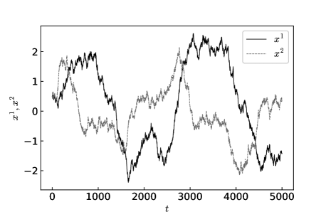
Figure 1: Sample paths of the stochastic equation (2) with the conditions (73)-(74).

4.2.1 ${\varSigma^{\prime}}_{\nu_{t+1}}^{-1}=0$

In this case, the counter term vanishes, $\delta_{c}V_{t+1}=0$ and the equation (36) implies that we are able to take $\bm{l}_{t+1}(\bm{x}_{t+1})$ as a linear function on $\bm{x}_{t+1}$.

As a first example, to constrain the stochastic process towards a target $\bm{d}_{t+1}$, we will consider the following effective potential as the cost function defined by a quadratic penalty function like (46):

$$V^{eff}_{t+1}(\bm{x}_{t+1}) =\frac{1}{2}\bm{l}_{t+1}(\bm{x}_{t+1})^{T}\varSigma_{\nu_{t+1}}^{-1}\bm{l}_{t+1}(\bm{x}_{t+1}),$$ (69)

$$\bm{l}_{t+1}(\bm{x}_{t+1}) =\bm{x}_{t+1}-\bm{d}_{t+1}.$$ (70)

This effective potential is a positive function and has a local minimum at $\bm{d}_{t+1}$. By the previous discussions, the principle of least action implies $\bm{\hat{x}}_{t+1|t+1}\rightarrow\bm{d}_{t+1}$, if we appropriately tune the parameter $\bm{g}_{t}$ and $\varSigma_{\nu_{t+1}}$. To numerically check this expectation, we will take the initial values as follows:

$$\bm{\hat{x}}_{0|-1} =\left(\begin{array}[]{c}0.5\\ 0.5\end{array}\right),$$ (73)

$$\bm{g}_{t}^{-1} =\begin{pmatrix}0.001&0\\ 0&0.001\end{pmatrix},$$ (74)

$$\hat{\varSigma}_{0|-1} =\begin{pmatrix}1&0\\ 0&1\end{pmatrix},$$ (75)

$$\varSigma_{\nu_{t+1}} =\begin{pmatrix}0.001&0\\ 0&0.0001\end{pmatrix},$$ (76)

$$\bm{d}_{t+1} =\left(\begin{array}[]{c}0.2\\ -0.1\end{array}\right),$$ (79)

$$\bm{H}_{t+1} =-\bm{1}_{2\times 2}.$$ (80)

Fig. 2 and Fig. 3 show sample paths of $\bm{x_{t}}$ and $\bm{u_{t}}$. These sample paths are given by the following steps. The initial control $\bm{u}_{0}$ is decided by substituting the conditions (73)-(80) for Eq. (57). $\bm{x}_{1}$ is sampled by the probability distribution (41) for the conditions. By repeating similar steps, we can obtain the sample paths. Fig. 2 and Fig. 3 indicate that the stochastic dynamics is controlled to the local minimum of $V^{eff}_{t+1}$.

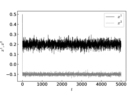
Figure 2: Sample paths by sampling from the probability distribution (41) with the potential (69) and the conditions (73)-(80).

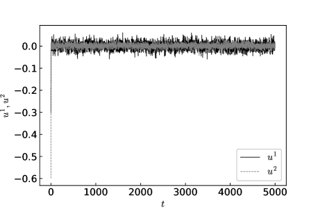
Figure 3: Control inputs corresponding to Fig. 2.

The second example is a constrained dynamics in $\bm{x}_{t+1}>\bm{0}$ and then the cost function is taken by a potential like barrier function:

$$V^{eff}_{t+1}(\bm{x}_{t+1}) =-\bm{a}^{T}\ln\bm{l}_{t+1}(\bm{x}_{t+1})$$ (81)

where $\bm{a}$ is a positive vector and

$$\ln\bm{l}_{t+1}(\bm{x}_{t+1}) =\begin{pmatrix}\ln l^{1}_{t+1}(\bm{x}_{t+1})&\ln l^{2}_{t+1}(\bm{x}_{t+1})\end{pmatrix}^{T}$$

$$=\begin{pmatrix}\ln x^{1}_{t+1}&\ln x^{2}_{t+1}\end{pmatrix}^{T}.$$ (82)

This potential monotonically increases towards $+\infty$ for $\bm{x}_{t+1}\rightarrow\bm{0}$ and decreases to $-\infty$ for $\bm{x}_{t+1}\rightarrow+\infty$ . It is expected that the potential constrains the stochastic processes to $\bm{x}_{t+1}>\bm{0}$. Using Eq. (35), $\varSigma_{\nu_{t+1}}$ is given by

$$\varSigma_{\nu_{t+1}} =\begin{pmatrix}(\hat{x}^{1}_{t+1|t})^{2}/a^{1}&0\\ 0&(\hat{x}^{2}_{t+1|t})^{2}/a^{2}\end{pmatrix}.$$ (83)

$\bm{H}_{t+1}$ is given by $\bm{H}_{t+1}=-\bm{1}_{2\times 2}$. The numerical simulation gives Fig. 4 and Fig. 5 by the same condition and manner with the first example, applying Eq. (83) and

$$\bm{a}=\begin{pmatrix}10&10\end{pmatrix}^{T}.$$ (84)

Fig. 4 and Fig. 5 show that the stochastic dynamics is constrained to $\bm{x}_{t+1}>\bm{0}$, by the potential as barrier function.

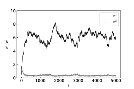
Figure 4: Sample paths by sampling from the probability distribution (41). The potential is given by Eq. (81) with Eq. (84). the sampling has used the conditions (73)-(80) in which $\varSigma_{\nu_{t+1}}$ is replaced by Eq. (83).

Figure 5: Control inputs corresponding to Fig. 4.

4.2.2 ${\varSigma^{\prime}}_{\nu_{t+1}}^{-1}\neq 0$

We will consider a case in which the cost function is given by a double well potential defined by Eq. (69) with

$$l^{m}_{t+1}(\bm{x}_{t+1}) =(x^{m}_{t+1}-d^{m}_{t+1})(x^{m}_{t+1}+d^{m}_{t+1})$$ (85)

where

$$\bm{d}_{t+1} =\left(\begin{array}[]{c}0.2[1+\tanh\{0.01(t-2500)\}]\\[10.0pt] 0.2[1+\tanh\{0.01(t-2500)\}]\end{array}\right).$$ (88)

The double well potential has the minima at $d^{m}_{t+1}$ or $-d^{m}_{t+1}$ by Eq. (85). The target $\bm{d}_{t+1}$ changes from $\begin{pmatrix}0&0\end{pmatrix}^{T}$ to $\begin{pmatrix}0.4&0.4\end{pmatrix}^{T}$ and then the minima of the double well potential dynamically deform, according to $\bm{d}_{t+1}$. Substituting Eq. (69) and Eq. (85) for Eq. (36), ${\varSigma^{\prime}}_{\nu_{t+1}}^{-1}$ is given by

$${\varSigma^{\prime}}_{\nu_{t+1}}^{-1}=\begin{pmatrix}2\hat{x}^{1}_{t+1|t}l_{t+1}^{1}(\hat{x}^{1}_{t+1|t})&0\\ 0&2\hat{x}^{2}_{t+1|t}l_{t+1}^{2}(\hat{x}^{2}_{t+1|t})\end{pmatrix}.$$ (89)

The numerical simulation gives Fig. 6 and Fig. 7 by the same condition and manner with the previous examples, replacing the corresponding conditions by

$$\bm{g}_{t}^{-1} =\begin{pmatrix}0.5&0\\ 0&0.5\end{pmatrix},$$ (90)

$$\varSigma_{\nu_{t+1}} =\begin{pmatrix}0.001&0\\ 0&0.001\end{pmatrix},$$ (91)

$$\bm{H}_{t+1} =\begin{pmatrix}-2\hat{x}^{1}_{t+1|t}&0\\ 0&-2\hat{x}^{2}_{t+1|t}\end{pmatrix}.$$ (92)

We find that the potential controls the stochastic processes along the dynamically changing minima.

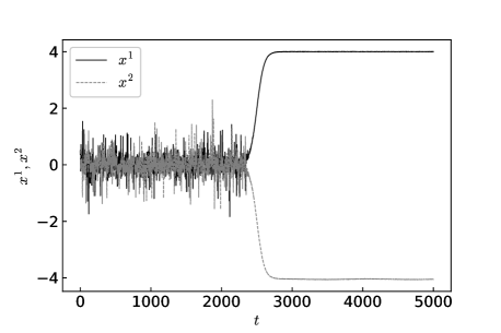
Figure 6: Sample paths by sampling from the probability distribution (41). The potential is given by Eq. (69) with Eq. (85). the sampling has used the conditions (73)-(80) in which $\bm{g}_{t}^{-1}$, $\varSigma_{\nu_{t+1}}$ and $\bm{H}_{t+1}$ are replaced by (90), (91) and (92), respectively.

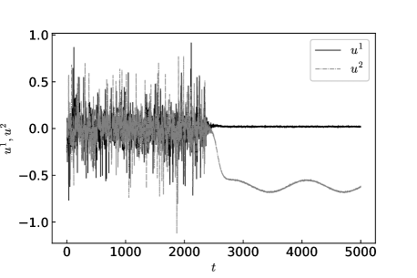
Figure 7: Control inputs corresponding to Fig. 6.

5 Conclusions

In this paper, we have proposed the discrete-time SQ using the weighted distribution as a novel and simple method to treat constrained dynamics of general Ito processes in engineering problems. The introduction of the weighted distribution in SQ has preserved the role of the path integral as the probability distribution and has naturally induced the potential term in the path integral, without imposing any assumption of the drift term. A second order approximation on the stochastic fluctuations to the path integral has given the difference equations representing the time-evolution of the expectation value and the covariance matrix for the stochastic systems. The difference equations have indicated that the potential term gives rise to forces constraining the stochastic dynamics. The difference equations has derived EKF by the potential function as the penalty function. Although the penalty function has involved observations as just external sources, we have also explained a case where such the stochastic interpretation of the observations is recovered as the typical definition of EKF. The potential function as a barrier or penalty function has been applied to model the nonlinear stochastic control. It has been numerically shown that the nonlinear stochastic processes can be constrained towards a minimum or a decreasing direction of the potential function.

For more realistic applications, how to accept constraints on control inputs induced from the potential term also remains to be considered. A hyperparameter optimization is also required since the stability of a given stochastic system depends on the hyperparameters. The computation on the covariance matrix has the high cost for a large-scale and high-dimensional system. Thus, how to reduce the computational cost is remaining problem to be solved in order to be more powerful tool for real world. It is also interesting to consider parameter estimation because EKF is able to estimate parameters of a machine learning model Singhal_Wu:1988 .

Appendix A Matrix inversion lemma and product rules for determinant

$A$ and $D$ are invertible square matrices, and $B$ and $C$ matrices may or may not be square. The matrix inversion lemma and the product rules for determinant are given as follows Simon:2006 :

$$(A+BD^{-1}C)^{-1}=A^{-1}-A^{-1}B(D+CA^{-1}B)^{-1}CA^{-1},$$ (93)

$$\left|\begin{array}[]{cc}A&B\\ C&D\end{array}\right|=|A-BD^{-1}C||D|=|A||D-CA^{-1}B|.$$ (96)

Appendix B Identities

Applying the matrix inversion lemma in Appendix A, we can show the following equations:

$$e^{-U_{t+\varDelta t}\varDelta t}p(x_{t+\varDelta t},t+\varDelta t)$$

$$=\frac{N_{t+\varDelta t}e^{-\mathcal{N}_{t+\varDelta t}\varDelta t}|\hat{\varSigma}_{t+\varDelta t|t+\varDelta t}|^{1/2}}{|\hat{\varSigma}_{t+\varDelta t|t}|^{1/2}}$$

$$\quad\times\frac{1}{(2\pi)^{m/2}|\hat{\varSigma}_{t+\varDelta t|t+\varDelta t}|^{1/2}}$$

$$\quad\times e^{-\frac{1}{2}(\bm{x}_{t+\varDelta t}-\bm{\hat{x}}_{t+\varDelta t|t+\varDelta t})^{T}\hat{\varSigma}_{t+\varDelta t|t+\varDelta t}^{-1}(\bm{x}_{t+\varDelta t}-\bm{\hat{x}}_{t+\varDelta t|t+\varDelta t})}$$

$$=P(x_{t+\varDelta t},t+\varDelta t)$$ (97)

where we have defined the following equations:

$$\bm{\hat{x}}_{t+\varDelta t|t+\varDelta t} =\bm{\hat{x}}_{t+\varDelta t|t}$$

$$\quad+(\hat{\varSigma}_{t+\varDelta t|t}^{-1}+\bm{H}_{t+\varDelta t}^{T}\varSigma_{\nu_{t+\varDelta t}}^{-1}\bm{H}_{t+\varDelta t}\varDelta t)^{-1}$$

$$\qquad\times\bm{H}_{t+\varDelta t}^{T}\bm{\nabla}_{\bm{l}_{t+\varDelta t}}V_{t+\varDelta t}\varDelta t$$ (98)

$$=\bm{\hat{x}}_{t+\varDelta t|t}$$

$$\quad+\hat{\varSigma}_{t+\varDelta t|t}\bm{H}_{t+\varDelta t}^{T}$$

$$\qquad\times(\varSigma_{\nu_{t+\varDelta t}}/\varDelta t+\bm{H}_{t+\varDelta t}\hat{\varSigma}_{t+\varDelta t|t}\bm{H}_{t+\varDelta t}^{T})^{-1}$$

$$\qquad\times\varSigma_{\nu_{t+\varDelta t}}\bm{\nabla}_{\bm{l}_{t+\varDelta t}}V_{t+\varDelta t},$$ (99)

$$\hat{\varSigma}_{t+\varDelta t|t+\varDelta t} =(\hat{\varSigma}_{t+\varDelta t|t}^{-1}+\bm{H}_{t+\varDelta t}^{T}\varSigma_{\nu_{t+\varDelta t}}^{-1}\bm{H}_{t+\varDelta t}\varDelta t)^{-1}$$ (100)

$$=\hat{\varSigma}_{t+\varDelta t|t}$$

$$\quad-\hat{\varSigma}_{t+\varDelta t|t}\bm{H}_{t+\varDelta t}^{T}$$

$$\qquad\times(\varSigma_{\nu_{t+\varDelta t}}/\varDelta t+\bm{H}_{t+\varDelta t}\hat{\varSigma}_{t+\varDelta t|t}\bm{H}_{t+\varDelta t}^{T})^{-1}$$

$$\qquad\times\bm{H}_{t+\varDelta t}\hat{\varSigma}_{t+\varDelta t|t},$$ (101)

$$|\varSigma_{\nu_{t+\varDelta t}}/\varDelta t +\bm{H}_{t+\varDelta t}\hat{\varSigma}_{t+\varDelta t|t}\bm{H}_{t+\varDelta t}^{T}|^{1/2}$$

$$\times|\varSigma_{\nu_{t+\varDelta t}}/\varDelta t|^{-1/2}|\hat{\varSigma}_{t+\varDelta t|t}|^{-1/2}$$

$$=|\hat{\varSigma}_{t+\varDelta t|t}^{-1}+\bm{H}_{t+\varDelta t}^{T}\varSigma_{\nu_{t+\varDelta t}}^{-1}\bm{H}_{t+\varDelta t}\varDelta t|^{1/2}.$$ (102)

Conflict of interest

The authors declare that they have no conflict of interest. This manuscript is an extended version of author’s presentation on stochastic process, when the author was working at Fringe81 Co., Ltd.. The manuscript is not related to the business.

References

- (1) H. Kleinert, Path Integrals in Quantum Mechanics, Statistics, Polymer Physics, and Financial Markets, World Scientific, Singapore, 2009.
- (2) H. Risken and T. Frank, The Fokker-Planck Equation: Methods of Solution and Applications, Springer-Verlag Berlin Heidelberg, Springer Series in Synergetics 18 (1996).
- (3) L. Peliti, Path integral approach to birth-death processes on a lattice, J. Physique 46, 1469-1483 (1985)
- (4) H. J. Kappen, A linear theory for control of non-linear stochastic systems, Phys. Rev. Lett. 95, 200201 (2005).
- (5) H. J. Kappen, Path integrals and symmetry breaking for optimal control theory, J. Stat. Mech. (2005) P11011.
- (6) R. F. Stengel, Optimal Control and Estimation, Dover Publications (1994).
- (7) E. Theodorou, J. Buchli and S. Schaal, Learning Policy Improvements with Path Integrals, Proceedings of the Thirteenth International Conference on Artificial Intelligence and Statistics, PMLR 9:828-835, 2010.
- (8) E. Theodorou, J. Buchli and S. Schaal, A Generalized Path Integral Control Approach to Reinforcement Learning, J. Mach. Learn. Res. 11 (2010) 3137-3181.
- (9) V. Linetsky, The Path Integral Approach to Financial Modeling and Options Pricing, Computational Economics 11: 129-163 (1998).
- (10) E. Baaquie, Quantum finance : path integrals and Hamiltonians for options and interest rate, Cambridge University Press, 2004.
- (11) G. Parisi and N. Sourlas, Random Magnetic Fields, Supersymmetry, and Negative Dimensions, Phys. Rev. Lett. 43, 744 (1979).
- (12) G. Parisi and W. Yong-shi, Perturbation Theory Without Gauge Fixing, Sientia Sinica 24 (1981) 483.
- (13) G. Parisi and N. Sourlas, Supersymmetric Field Theories and Stochastic Differential Equations, Nucl. Phys. B 206, 321 (1982).
- (14) G. Parisi, Statistical Field Theory (Advanced Book Classics), CRC Press (1998).
- (15) P. H. Damgaard and H. Huffel, Stochastic Quantization, Phys. Rept. 152, 227 (1987).
- (16) M. Namiki, I. Ohba, K. Okano, Y. Yamanaka, A. K. Kapoor, H. Nakazato and S. Tanaka, Stochastic quantization, Lect. Notes Phys. Monogr. 9, 1-217 (1992).
- (17) F. Cooper, A. Khare and U. Sukhatme, Supersymmetry and quantum mechanics, Phys. Rept. 251, 267-385 (1995).
- (18) M. Namiki, Basic Ideas of Stochastic Quantization, Progress of theoretical physics. Supplement (111) 1-41 (1993).
- (19) J. Dash, Path Integrals and Options, Part I, CNRS Preprint CPT-88/PE.2206, (1988).
- (20) J. Dash, Path Integrals and Options, Part II, CNRS Preprint CPT-89/PE.2333, (1989).
- (21) J. W. Dash, Quantitative Finance and Risk Management: A Physicist’s Approach, World Scientific Pub Co Inc (2004).
- (22) Y. Nakayama, Gravity Dual for Reggeon Field Theory and Non-linear Quantum Finance, Int. J. Mod. Phys. A24: 6197-6222 (2009).
- (23) R. Fletcher, Practical Methods of Optimization, Second edition, John Wiley & Sons (2000)
- (24) J. Nocedal and S. J. Wright, Numerical Optimization, Springer Series in Operations Research and Financial Engineering, Springer; 2nd ed. (2006)
- (25) C. Radhakrishna Rao, On Discrete Distributions Arising out of Methods of Ascertainment, in Classical and Contagious Discrete Distributions, G. P. Patil, ed. Pergamon Press and Statistical Publishing Society, Calcutta, pp. 320-332 (1965).
- (26) C. Radhakrishna Rao, Weighted Distributions Arising Out of Methods of Ascertainment: What Population Does a Sample Represent?, In: Atkinson A.C., Fienberg S.E. (eds) A Celebration of Statistics. Springer, New York, NY (1985).
- (27) G. P. Patil and C. R. Rao, Weighted Distributions and Size-Biased Sampling with Applications to Wildlife Populations and Human Families, Biometrics 34, no. 2 (1978): 179-89.
- (28) D. Simon, Optimal State Estimation: Kalman, H Infinity, and Nonlinear Approaches, Wiley-Interscience, 2006.
- (29) S. Srkk, Bayesian Filtering and Smoothing, Cambridge University Press, 2013.
- (30) S. Singhal and L. Wu, Training Multilayer Perceptrons with the Extended Kalman Algorithm, NIPS’88 Proceedings of the 1st International Conference on Neural Information Processing Systems, Pages 133-140