New technique to measure the cavity defects of Fabry-Perot interferometers

Abstract

Context. Several astronomical instruments, for both nighttime and solar use, rely on tunable Fabry-Perot interferometers (FPIs). Knowing the exact shape of the etalons’ cavity is crucial for assessing the overall instrumental transmission profile and its possible variations during the tuning process.

Aims. We aim to define and test a technique to accurately measure the cavity defects of air-spaced FPIs, including distortions due to the spectral tuning process that are typical of astronomical observations. We further aim to develop a correction technique to maintain the shape of the cavity as constant as possible during the spectral scan. These are necessary steps to optimize the spectral transmission profile of a two-dimensional spectrograph (polarimeter) using one or more FPIs in series, and to ensure that the spectral transmission profile remains constant during typical observing conditions.

Methods. We devised a generalization of the techniques developed for the so-called phase-shifting interferometry to the case of FPI. This measuring technique is applicable to any given FPI that can be tuned via changing the cavity spacing ($z$-axis), and can be used for any etalon regardless of the coating’ reflectivity. The major strength of our method is the ability to fully characterize the cavity during a spectral scan, allowing for the determination of scan-dependent modifications of the plates. We have applied the measuring technique to three 50 mm diameter interferometers, with cavity gaps ranging between 600 $\mu$m and 3 mm, coated for use in the visible range.

Results. The technique developed in this paper allows us to accurately and reliably measure the cavity defects of air-spaced FPIs, and of their evolution during the entire spectral scan. Our main, and unexpected, result is that the relative tilt between the two FPI plates varies significantly during the spectral scan, and can dominate the cavity defects; in particular, we observe that the tilt component at the extremes of the scan is sensibly larger than that at the center of the scan. Exploiting the capability of the electronic controllers to set the reference plane at any given spectral step, we then develop a correction technique that allows the minimization of the tilt during a complete spectral scan. The correction remains highly stable over long periods, well beyond the typical duration of astronomical observations.

1 Introduction

Astronomical instruments based on Fabry-Perot interferometers (FPIs) have proved a flexible and efficient way to perform imaging spectroscopy and polarimetry. In nighttime astronomy, the first system of this kind, and one of the most successful to date, has been the Taurus Tunable Filter, which operated for a decade on the Anglo-Australian Telescope and the William Herschel Telescope (Bland-Hawthorn & Jones, 1998; Jones et al., 2002). Building on this experience, a number of similar instruments have been successively developed and used at a variety of telescopes. These currently include OSIRIS at the GTC 10-m telescope (Cepa, 2013; Cepa et al., 2013); the Maryland-Magellan Tunable Filter MMTF (Veilleux et al., 2010); the FP system for the Robert Stobie Spectrograph on SALT (Rangwala et al., 2008; Williams et al., 2016). New instruments are also being planned, such as the Brazilian Tunable Filter Imager (BTFI2) for the SOAR telescope (Quint et al., 2018), or a system for detection of molecular oxygen in exoplanets’ atmosphere operating on forthcoming ELTs (Ben-Ami et al., 2018).

Among the most-used instruments in solar physics are the dual FPI CRisp Interferometric SpectroPolarimeter (CRISP, Scharmer et al., 2008) and CHROMIS (Scharmer 2019, in prep.), both at the Swedish Solar Tower (SST); the Triple Etalon SOlar Spectrometer (TESOS, Kentischer et al., 1998; Tritschler et al., 2002) at the German Vacuum Tower Telescope (VTT); the dual FPI Italian Interferometric BIdimensional Spectrometer installed at the Dunn Solar Telescope of the National Solar Observatory (IBIS, Cavallini, 2006); the Imaging Magnetograph eXperiment (IMaX) flown on the Sunrise I and II balloons (Martínez Pillet et al., 2011); and the Gregor Fabry Perot Interferometer currently operating at the German GREGOR 1.5 m telescope in Tenerife (GFPI, Puschmann et al., 2012). The Visible Tunable Filter is currently under construction, planned for installation at the upcoming 4-m aperture solar telescope DKIST (Schmidt et al., 2016; Warner et al., 2018).

Most of these FPIs are air-spaced, and spectrally tunable by rapidly changing the cavity spacing via piezo-electric actuators. A peculiar characteristic of the FPIs used for solar instruments is their very high spectral resolution ($R>$100,000), which allows precise spectropolarimetry of narrow spectral lines. This requirement translates into FPI gaps on the order of one to few millimeters, in contrast with cavities of few tens of microns, for the majority of nighttime instruments. Instruments using these FPI rapidly and repeatedly change the gap of the FPI over a wide range to select different transmission wavelengths and thus perform a spectral scan.

The overall transmission profile of these instruments, and its possible variation with wavelength and across the field of view (FOV) are important parameters in order to properly interpret the observed spectral and polarimetric profiles. In particular, the widely used technique of spectral inversions as a way to derive solar atmospheric parameters from the shape of the observed spectral lines (Ruiz Cobo & del Toro Iniesta, 1992; de la Cruz Rodríguez & van Noort, 2017) requires an exact knowledge of the shape of the instrumental transmission profile, as details like asymmetries in the observed Stokes profiles might reveal gradients in physical quantities such as velocity, or magnetic field intensity and direction. As an example, an earlier work by Reardon & Cavallini (2008) assesses the influence of the cavity errors of the FPIs employed in IBIS on the overall instrumental profile. By using simulated spectral profiles of a photospheric line, they show how using the “nominal”, ideal instrumental profile rather than the true one, could introduce uncertainties in the convolved line profiles comparable with the expected signal, for example for the case of weak polarization signals (at the level of few $\times 10^{-3}$ the continuum intensity). For instruments using the telecentric mount, defect-induced wavelength shifts across the FOV are also an important factor to consider, as they compound other issues such as the need to obtain the highest possible spatial resolution via image reconstruction techniques (e.g., de la Cruz Rodríguez et al., 2015).

The cavity errors of a FPI can be decomposed in large and small scale components. The small-scale errors, which have negligible size with respect to the aperture of the FPI plates, are essentially due to the microroughness of the glass substrate and/or the coating. The large-scale errors, meaning those with sizes comparable to the size of the plates, can be due to a variety of factors. These include manufacturing errors; tension on the plates due to the coating; pre-load stresses introduced in the assembly of the FPIs; pressure exerted by the actuators; gravity; and, most important, a tilt of the plates, that is, deviations from the parallelism of the two planes best fitting the plates’ shape. These large-scale errors are best described with a series of Zernike polynomials (Wyant & Creath, 1992).

While most of the cavity errors are permanently determined during the fabrication phase, the relative tilt of the two plates composing the cavity can be minimized and in principle eliminated during operations, if an accurate defects map is available, and the system includes a set of actuators that can act differentially on the plates. The latter is the case for most of the FPIs used in operational astronomical instruments; to date, most of the tunable FPIs used in astronomy are capacity-controlled devices produced by IC Optical Systems Ltd. (ICOS, http://www.icopticalsystems.com/).

Various authors have described ways to measure and minimize the relative tilt of FPI’ plates, most often as part of the (daily) instrumental calibration at the telescope. Jones & Bland-Hawthorn (1998) and Mickey (2004) proposed using differential measurements across separate quadrants of the etalons’ plates, while Veilleux et al. (2010) used a scan of both axes of movement to identify the position where the spectral profile of a bright emission line from an arc lamp is the narrowest. The same technique was also adopted for the SALT RSS FP system (Rangwala et al., 2008) but added significantly to the downtime of the instrument. In a follow up work, Williams et al. (2016) described how the instrumental setup could be accelerated by exploiting the correlation of the tilt parameters with the position of the center of a calibration interference ring. A similar idea was presented by Denker & Tritschler (2005), who observe how the tip-tilt parameters characterizing the cavity are linearly dependent on the voltage defining either axis of movement; a single measure of the cavity shape (defined in terms of Zernike polynomial, see below) would then be sufficient to derive the optimal settings for minimizing the tilt. For the case of IBIS, Cavallini (2006) describes the procedure adopted to minimize the parallelism error of each FPI separately using the calibration channel of the instrument, which includes a laser source and a diffuser, coupled with a set of lenses that can image the cavities of the two FPIs (one at a time) onto the science camera.

Although rapid and efficient, most of these procedures are based on approximate estimates of the best orientation of the plates, and are often amenable to subjective interpretation. For example, Reardon & Cavallini (2008) perform a full analysis of the cavity errors of IBIS and showed that after the manual tilt minimization procedure they could still measure a significant residual tilt, with peak-to-valley ($PV$) values in the range

$$\centering 1.24\leavevmode\nobreak\ $nm$\leavevmode\nobreak\ \leq PV\leq 3.17\leavevmode\nobreak\ $nm$.\@add@centering$$ (1)

For a single FPI in a collimated mount, such a residual tilt produces a broadening of the transmission profile approximately expressed by the relation

$$\frac{\ \ \delta FWHM\ \ }{FWHM}=\sqrt{\ \ 1+3R\ \Bigg{[}\frac{\pi\ \Delta t_{M}}{\ \ \lambda\ (1-R)\ \ }\Bigg{]}^{2}\ \ }-\ 1,$$ (2)

where FWHM is the full width at half maximum of the transmission profile of an ideal interferometer (no cavity defects); $\Delta t_{M}$ is the $PV$ value of the tilt; R the reflectivity of the plates, and $\lambda$ the wavelength. If in Eq. 2 we assume R = 0.95 (typical of solar instruments) and $\lambda$=550 nm, we obtain a broadening of 3% for $\Delta t_{M}$ =1.24 nm, and of 17% for $\Delta t_{M}$ =3.17 nm. In a telecentric mount, the same values of residual tilt would introduce shifts of the spectral transmission profile on the order of 200-500 ms^-1 (at visible wavelengths) over the whole field of view. These are already significant degradations of the ideal instrumental profile but, even more importantly, they will compound in a non-trivial manner, in the common case of multiple interferometers operating in series, for example decreasing the overall transmission or changing the shape of the combined profile (e.g., Williams et al., 2016; Ben-Ami et al., 2018).

A more objective characterization of the cavity errors of FPI, and a more accurate way to control the plate parallelism, appears thus necessary. In the present paper, we have followed the approach of Denker & Tritschler (2005) and Reardon & Cavallini (2008), to fully describe the cavity shape of a Fabry Perot Interferometer in terms of Zernike polynomials. Extending their analysis, however, we explicitly consider the possibility that the cavity errors might change during the full spectral scan. This is motivated by two distinct factors. First, some deformation of the cavity can be expected when it is pushed far from the central gap spacing, because of the relatively large excursions of the piezoelectrics and the FPI’s plates during the tuning process, while confined in an essentially rigid, overall hardware structure. The extremes of the spectral scan can often be approached when exploring a variety of astronomical problems, so this effect is worth investigating. Second, even though the overall alignment of the FPI’s plates is supposed to be maintained by the balancing action of the capacitance bridge used to drive the piezo-electric actuators (see e.g., Sect. 4), our measurements on several ICOS FPIs, described below, show that this might not be the case. To our knowledge, this is the first time that possible changes of the cavity errors during the spectral scan are explicitly taken into account.

In Sect. 2 we present a novel procedure, developed and tested at the Optical Measurements and Testing Laboratory of the Italian National Center for Research (CNR - INO), to measure the cavity defects of any given FPI of up to 150 mm diameter. In Sect. 3 we describe in detail the application of this technique to an existing 50 mm diameter FPI (model ET50, fabricated by ICOS) and the ensuing results. We applied the same technique on two other ICOS ET50, obtaining consistent results; we provide these in Appendix A. As shown in Sect. 3, the plates’ tilt, and hence the transmission profile, can indeed vary significantly within the spectral scan; in Sect. 4 we further define and test a procedure to minimize and stabilize the tilt during a full spectral scan, discussing the resulting effects on the instrumental transmission profile. Finally, we present our discussion and conclusions in Sect. 5.

2 Characterizing the FPI cavity

2.1 The measuring technique: analytical formulation

Figure 1: Optical cavity of a non-ideal Fabry-Perot interferometer. $n$ is the step position within the spectral scan ($n\in[-2047,2048]$ for a typical ICOS controller. See also Eq. 3 below).

Figure 1 shows a schematic non-ideal, air-spaced Fabry-Perot interferometer, where the two plates that combine to form the actual cavity are not perfect parallel planes. The defects are enhanced for clarity. In all of our analyses, we have assumed that the index of refraction of the air within the etalon remains constant; this holds for our laboratory measurements but also for typical instruments (e.g., IBIS) where the interferometers are pressure- and temperature-controlled (to within $<$ 0.1^∘ C in the case of IBIS).

We call the cavity spacing D₀, defined as the average of the distance between the single plate points, over the whole surface. A system of actuators (three in the case of ICOS ET50, see Fig. 11 below) allows us to change the plates’ separation along the longitudinal axis ($z$ in Fig. 1); this is how spectral tuning is achieved in most current instruments. Using a proximity sensor system, the actuators’ controller shifts one plate with respect to the other in constant steps, of size $\Delta$, within the range [ D${}_{0}-\big{(}2^{(N-1)}-1\big{)}\cdot\Delta$, D${}_{0}+\big{(}2^{(N-1)}\big{)}\cdot\Delta$ ], where $N$ is the digital resolution of the controller. For the case of high spectral resolution ICOS interferometers, typical values are: D₀ = one to few mm; $N$ = 12; and $\Delta$ = 0.5 nm.

Using the reference system $(x,y,z)$ depicted in Fig. 1, with the $z$ axis coinciding with the optical axis of the interferometer, the distance $D(x,y,n)$ between any two points of coordinates $(x,y)$ on the plates is given by:

$$D(x,y,n)\ =\ D_{0}\ +\ n\cdot\Delta\ +\ F(x,y,n),$$ (3)

where $n\in\big{[}-\big{(}2^{(N-1)}-1\big{)},\ 2^{(N-1)}\ \big{]}$ is any given step of the scan, and the map $F(x,y,n)$ includes all the cavity errors. Assuming that $F(x,y,n)$ is a slowly varying function of $n$, we can write:

$$F(x,y,n)\ \simeq\ F_{0}(x,y)\ +\ F_{1}(x,y)\cdot n\ +\ F_{2}(x,y)\cdot n^{2},$$ (4)

where the term $F_{0}(x,y)$ includes all the static cavity errors apart from those introduced by the moving actuators, encoded in $F_{1}(x,y)$ and $F_{2}(x,y)$.

Substituting Eq. 4 in Eq. 3 we obtain:

$$D(x,y,n)\ =\ D_{0}\ +\ \big{[}\Delta+F_{1}(x,y)\big{]}\cdot n\ +\ F_{2}(x,y)\cdot n^{2}\ +\ F_{0}(x,y).$$ (5)

To first order in $n$, for each cavity pixel $(x,y)$ the spectral scan thus results in a different step size, $\Delta_{1}$ given by:

$$\Delta_{1}\ =\ \Delta\ +\ F_{1}(x,y).$$ (6)

Further, since the map of cavity defects $M(x,y,n)$ is defined (apart from an additive constant) by:

$$M(x,y,n)\ =\ D(x,y,n)\ -\ D(0,0,n)$$ (7)

using Eq. 5 , we obtain:

$$M(x,y,n)\simeq\ \big{[}F_{1}(x,y)-F_{1}(0,0)\big{]}\cdot n\ +\ \big{[}F_{2}(x,y)-F_{2}(0,0)\big{]}\cdot n^{2}\\ +\ \big{[}F_{0}(x,y)-F_{0}(0,0)\big{]}.$$ (8)

By illuminating the FPI with a monochromatic, collimated beam along the $z$ axis, and assuming negligible absorption in the cavity, the transmitted $I_{T}(x,y,n)$ and reflected $I_{R}(x,y,n)$ intensities are given by the well known Airy relations (e.g., Vaughan, 1989):

$$I_{T}(x,y,n)\ =\ \frac{I_{0}(x,y)}{\ \ 1+\dfrac{2R}{\ \ (1-R)^{2}\ \ }\bigg{[}1-\cos\bigg{(}\dfrac{4\pi}{\lambda}D(x,y,n)\bigg{)}\bigg{]}\ \ }$$ (9)

$$I_{R}(x,y,n)=I_{0}(x,y)-I_{T}(x,y,n)$$ (10)

where $I_{0}(x,y)$ is the incident intensity, $\lambda$ is the wavelength, and $R$ the reflectivity of the plates (a slowly varying function of $\lambda$).

If we measure the intensity of the transmitted and reflected beams with a 2-D detector (e.g., a CCD), as $n$ is stepped through increasing values every pixel $(x,y)$ will experience a succession of interference orders with modulation:

$$K_{T}=\frac{(I_{T})_{max}-(I_{T})_{min}}{(I_{T})_{max}+(I_{T})_{min}}=\frac{2R}{1+R}\\ K_{R}=\frac{(I_{R})_{max}-(I_{R})_{min}}{(I_{R})_{max}+(I_{R})_{min}}=1\ \ \ (I_{R})_{min}=0$$ (11)

$I_{T}$ and $I_{R}$ can be written as

$$I_{T}(x,y,n)\ =C(x,y)\ +\\ \frac{A(x,y)}{\ \ 1+B(x,y)\cdot\Big{\{}1-\cos\Big{[}\alpha(x,y)\cdot n+\beta(x,y)\cdot n^{2}+\gamma(x,y)\Big{]}\Big{\}}}$$ (12)

$$I_{R}(x,y,n)\ =C(x,y)\ +\ A(x,y)\cdot\Bigg{\{}\ \ 1\ -\\ \frac{1}{\ \ 1+B(x,y)\cdot\Big{\{}1-\cos\Big{[}\alpha(x,y)\cdot n+\beta(x,y)\cdot n^{2}+\gamma(x,y)\Big{]}\Big{\}}}\Bigg{\}}$$ (13)

where:

$$\begin{split}\alpha(x,y)\ &=\ \frac{4\pi}{\lambda}\cdot\big{[}\Delta+F_{1}(x,y)\big{]}\\ \beta(x,y)\ &=\ \frac{4\pi}{\lambda}\cdot F_{2}(x,y)\\ \gamma(x,y)\ &=\ \frac{4\pi}{\lambda}\cdot\big{[}D_{0}+F_{0}(x,y)\big{]}\end{split}.$$ (14)

In Eqs. 12 and 13, the matrix $A(x,y)$ describes possible spatial variations of both the incident beam’s intensity and the gain by each CCD pixel; matrices $B(x,y)=\tfrac{2R}{(1-R)^{2}}$ and $C(x,y)$ describe spatial variations of the plates’ reflectivity and pixels’ offset, respectively.

Let us assume we acquired an interferogram $I_{R}(x,y,n)$ of the reflected beam (alternatively, of the transmitted beam) for every step $n$ of the spectral scan. By fitting the intensity measured in each pixel $(x,y)$ as a function of $n$ using Eq. 13, we can determine the six matrices: $A(x,y)$, $B(x,y)$, $C(x,y)$, $\alpha(x,y)$, $\beta(x,y)$ and $\gamma(x,y)$, and hence the way in which the map of cavity errors evolves during the spectral tuning. In fact, assuming that the $PV$ value of the cavity errors is $<\lambda/2$, substituting Eq. 14 in Eq. 8 we obtain:

$$M(x,y,n)=H\cdot\frac{\lambda}{4\pi}\cdot\Bigg{\{}\\ \Big{[}\alpha(x,y)-\alpha(0,0)\Big{]}\cdot n+\Big{[}\beta(x,y)-\beta(0,0)\Big{]}\cdot n^{2}+\Big{[}\gamma(x,y)-\gamma(0,0)\Big{]}\Bigg{\}}$$ (15)

with H an “inversion” factor that can be either $[+1,-1]$. In the first case (H=$+1$), $M(x,y,n)$ describes the map of the cavity defect (apart from an additive value), while in the second (H=$-1$) $M(x,y,n)$ describes the shape of the surface of one of the plates, assuming the other is a perfect plane. This is equivalent to saying that the knowledge of $I_{R}$ or $I_{T}$ is not sufficient to separately determine the shape of the two surfaces composing the cavity.

The technique to measure cavity defects that we describe here below is based on Eqs. 12-15, and can be considered as a generalization of the techniques developed within the so-called phase-shifting interferometry (Schreiber & Bruning, 2007) to the case of FPIs. The phase-shifting technique has been developed within the framework of optical testing, and is usually employed to characterize cavities that: $i$) have a very low reflectivity $(R\simeq 0.04)$, so that the interference orders are essentially sinusoidal; and $ii$) are supposed to have constant shape throughout the spectral scan. Only recently some modifications have been proposed to the classical technique, that allow it to be used in cases when the tilt of the cavity varies within the spectral scan (Deck, 2014). Our own technique expands on these efforts, in the sense that it can be used for any value of the reflectivity R, and can fully characterize the cavity during a spectral scan, hence not only measuring the tilt variations, but also scan-dependent modifications of the plates (Sections 3 and 4 below). These features make our technique extremely useful for the characterization of astronomical Fabry-Perot, as R can be rather large $(R>0.8)$, and the residual tilts be of large relevance for accurate spectroscopy (see the discussion in the Introduction of this paper).

Finally, it is trivial to prove that our technique is a generalization of that used in Denker & Tritschler (2005) and Reardon & Cavallini (2008). These authors derive the value of the step $\Delta$ by measuring the average number of steps between two consecutive maxima of the $I_{T}$ curve, and imposing that the distance between the maxima is $\lambda/2$, with $\lambda$ the wavelength of the laser. For every pixel $(x,y)$ of the final image they then identify (for a given interference order) the position $n_{m}(x,y)$ of the local $I_{T}$ maximum; to this end Denker & Tritschler (2005) use a gaussian fit of the intensity curve, while Reardon & Cavallini (2008) employ a center of gravity method.

The map of cavity defects $M_{0}[x,y,n_{m}(0,0)]$ corresponding to the mid-step of the scan, $n_{m}(0,0)$, is then computed using:

$$M_{0}\Big{[}x,y,n_{m}(0,0)\Big{]}\ =\ H\cdot\Delta\cdot\Big{[}n_{m}(0,0)-n_{m}(x,y)\Big{]}$$ (16)

with $H$ defined as in Eq. 15. By comparing with Eq. 12, we see that the matrix $n_{m}(x,y)$ is defined by:

$$\alpha(x,y)\cdot n_{m}(x,y)+\beta(x,y)\cdot n_{m}^{2}(x,y)+\gamma(x,y)=2k\pi$$ (17)

with $k=0,\pm 1,\pm 2,...$ depending on the interference order. If we derive $\gamma(x,y)$ from Eq. 17, and substitute it in Eq. 15, using Eq. 14 we obtain:

$$M\Big{[}x,y,n_{m}(0,0)\Big{]}\ =\ H\cdot\Bigg{\{}\Big{[}\Delta+F_{1}(x,y)\Big{]}\cdot\Big{[}n_{m}(0,0)-n_{m}(x,y)\Big{]}+\\ F_{2}(x,y)\cdot\Big{[}n_{m}^{2}(0,0)-n_{m}^{2}(x,y)\Big{]}\Bigg{\}}.$$ (18)

For $F_{1}(x,y)=F_{2}(x,y)\equiv 0$ Eq. 18 is equal to Eq. 16, thus demonstrating that our technique is equivalent to the earlier ones if we neglect the possibility of cavity distortions during the scan.

2.2 Measuring technique: experimental setup

Figure 2: Optical setup adopted to measure the reflected intensity from a Fabry-Perot interferometer FPI. AT = Attenuator; SF = Spatial Filter; PBC = Polarizing Beam Splitter Cube; P = $\lambda/4$ Plate; C = Collimator; FPI = Fabry-Perot interferometer; A = Aperture (diaphragm); L = Imaging Lens; RD = Rotating Diffuser Disk; ZL = Zoom Lens; D = Detector.

In Fig. 2 we show the optical setup adopted to measure the intensity reflected by a FPI. The spatial filter (SF) produces a point-like monochromatic source, in the focus of the collimator (C). The laser beam is linearly polarized, and oriented so as to be completely reflected by the polarizing beam splitter cube (PBC). The beam is then directed through the $\lambda/4$ plate (P), oriented at 45^∘ with respect to the direction of polarization, thus emerging circularly polarized. The beam reflected by the FPI, after passing through the collimator and the quarter-wave plate is again linearly polarized, but at 90^∘ with respect to the original direction, and is hence transmitted by the PBC, and focused on the diaphragm A. The diaphragm is necessary to filter out all the spurious fringes produced by all the surfaces within the optical path apart from the internal surfaces of the FPI. The lens L remaps the optical cavity of the FPI onto a rotating diffuser disk, which is needed to remove the speckle field introduced by the laser. Finally, the zoom lens (ZL) images the cavity onto a 512$\times$512 camera (D).

The FPI transmitted intensity could be measured with an analogous, simpler optical setup, but the measure of the reflected intensity is more versatile. Indeed, while for high values of reflectivity (R $>$ 0.9) the two setups would be equivalent, for low values (R $\sim$ 0.04) the measure of the reflected intensity is more advantageous since the modulation of the transmitted beam is about 8%, vs. the 100% of the reflected beam (Eq. 11). Examples of low reflectivity cases include an uncoated cavity, useful to characterize the fabrication errors separately from the coating ones (R $\sim$ 4%, typical of the air-glass system), or a coated cavity optimized for wavelengths far from that of the laser used for the measures (e.g., infrared-optimized coatings).

3 Experimental data: the case study of an ICOS ET50

As a case study, we applied the technique described in Sect. 2 to the measure of the cavity defects of a servo-stabilized interferometer system, composed of a ICOS FPI ET50 FS and its CS100 controller. The FPI ET50 and CS100 were previously used as the main components of the Interferometric Panoramic Monochromator installed at the THEMIS telescope (IPM, Cavallini, 1998; Berrilli et al., 1999). The relevant characteristics of the system are given in Table 1.

Table 1: Servo-Stabilized Interferometer System characteristics

Fabry-Perot Interferometer
Manufacturer	IC Optical Systems
Type	ET50 FS
Aperture	50 mm
Material	Fused Silica
	(minimal inhomogeneity)
Plate Wedge	20 arcmin
Cavity Spacing	3.000 mm $\pm\sim$0.005 mm
Coating	Multilayer broadband
Wavelength range	400  nm $-$ 700  nm
Estimated cavity errors	$\lambda$ / 100 (PV $@$ 632.8 nm, after
	coating, over central 35 mm)
Nominal Reflectance	95% $\pm$ 3%
Estimated Step $(\Delta)$	$\sim$0.46 nm
Tilt Control Estimated precision (X, Y)	$\sim$1.4 $\cdot 10^{-3}$ arcsec
Controller
Manufacturer	IC Optical Systems
Type	CS100
Digital Resolution (N)	12 bits / 4096 steps

The measurements were performed at the “Laboratorio di Misure e Collaudi Ottici” of the Italian Istituto Nazionale di Ottica (INO), in a clean room with constant temperature and humidity (T=20$\pm$0.1 C, RH=45% $\pm$ 5%). This ensured that the index of refraction of the air between the FPI plates remained constant throughout the measures.

The optical setup of Fig. 2 was realized using a phase-shifting interferometer GPI-XP of Zygo-Ametek (www.zygo.com), that outputs a collimated HeNe ($\lambda$=632.8 nm) laser beam of 100 mm diameter (a 150 mm beam expander is also available, and can be used to extend the measures to larger format FPI). The ET50 is positioned in front of the GPI-XP so that the $z$-axis of the cavity is horizontal (perpendicular to gravity), and aligned so that its optical axis coincides with that of the collimator. The capability of the GPI-XP to introduce a phase-shift on the beam was disabled; rather, the GPI-XP was used simply as a collimator and to acquire (with 8 bit digitization) the light reflected from the ET50. All the elements of the setup depicted in Fig. 2, apart from the FPI, are contained in the GPI-XP case. Fig. 3 shows a typical interferogram observed at the central position ($n$=0) of the spectral scan. The acquisition software selects a central circular section of the image, with 325 pixel diameter; this corresponds to the central part of the pupil of the ET50, with a diameter of 35 mm (108 $\mu$m / pixel). Comparing Fig. 3 with the equivalent images in Reardon & Cavallini (2008) we observe a diminished “granularity” in the cavity errors in our case; this could be due either to the reduced dimensions and dynamic range of our detector, or to an intrinsic difference in the property of the coating. The corresponding maps derived for the case of the two additional NSO FPIs show variations on smaller spatial scales (see figures in Appendix); as a result, we favor the second hypothesis.

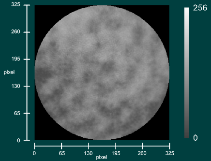
Figure 3: Typical interferogram of the ET50 measured in reflection. $\lambda$ =632.8 nm, $n$=0

Using the resident software of the GPI-XP (MetroScript Programming Language) it is possible to simultaneously manage remotely both the GPI-XP and the CS100 controlling the ET50. To measure the cavity defects, we developed a script that incrementally changes the distance between the FPIs’ plates by one step at a time ($\Delta$, see Table 1), and then acquires the corresponding interferogram with the GPI-XP. The complete spectral scan (4096 steps) takes approximately 24 minutes. The interferogram’s acquisition starts about 360 ms after each incremental step is applied; this is much longer than the damping time of the cavity ($\leq$ 20 ms) that we measured in the laboratory.

3.1 Fringe fitting

In Fig. 4 we show, in arbitrary units, the value of the intensity recorded in the central pixel of the camera during the complete spectral scan of 4096 steps. Over a complete spectral scan the distance between the plates of the ET50 increases about 1.9 $\mu$m, and every CCD pixel observes six interference orders. Figure 5 provides an enlarged view of the central interference order.

In both Figs 4 and 5 the red points represent the experimental data, while the solid black line represents the best fit of Eq. 13 (to perform the fit we used the routine $\it{mrqmin}$ of Numerical Recipes based on the Levenberg-Marquardt method). It is important to remark that the fit includes all the interference orders at once, and not only the central one as in Denker & Tritschler (2005) and Reardon & Cavallini (2008).

Also visible in the Figures, Eq. 13 describes the experimental data very well; indeed, for every pixel $(x,y)$ the rms value of the differences between the observed and fitted intensity, normalized to the value $A(x,y)$ (Eqs. 12 and 13) is limited to 1% – 3%, thus validating the assumption contained in Eq. 4. In particular, we find that the step $\Delta_{1}$ defined in Eq. 6 and derivable from $\alpha(x,y)$ via the equation:

$$\centering\Delta_{1}(x,y)=\lambda/(4\pi)\times\alpha(x,y),\@add@centering$$ (19)

changes sensibly within the (recorded) cavity, having values that vary between 0.4605 nm and 0.4623 nm. Although the variation is only of order 0.5%, note that its effect is amplified by the factor $n$ (Eq. 15).

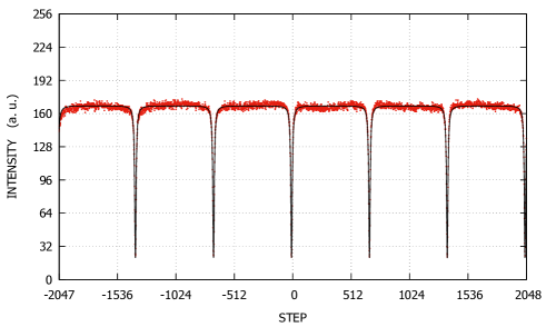
Figure 4: Intensity recorded in the central pixel of the images, during a complete spectral scan of 4096 steps. Red points: recorded data points; black line: fit using Eq. 13

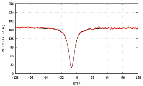
Figure 5: Detail of the central order of Fig. 4

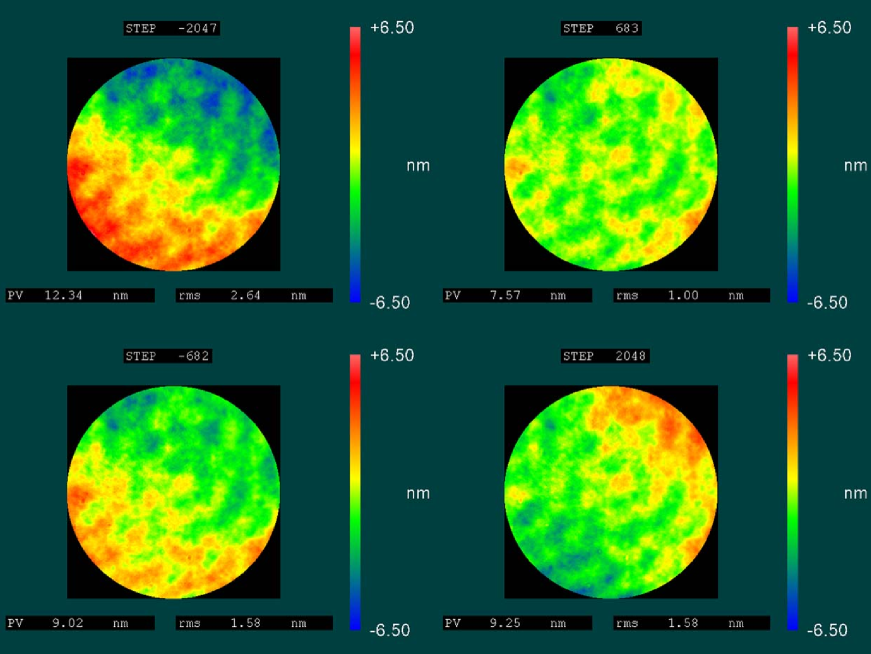
Figure 6: Maps of the cavity errors $M(x,y,n)$ for four values of the spectral step $n$, as indicated in the top of each map. A video of the cavity error maps for every spectral step is available in the online version of this paper (Fig6.mp4)

3.2 Effects of spectral tuning

The fit of Figs. 4 and 5 was performed independently for the intensity curves acquired in each spatial pixel $(x,y)$. Thus, after determining the six maps $A(x,y)$, $B(x,y)$, $C(x,y)$, $\alpha(x,y)$, $\beta(x,y),$ and $\gamma(x,y)$, we could calculate the map of the cavity errors $M(x,y,n)$ for every step of the scan (assuming H=$-$1; see Eq. 15). Figure 6 shows $M(x,y,n)$ for four different values of $n$ ($n$=$-$2047,$-$682,+683,+2048), while the corresponding animation (available in the online version of the paper), displays the map for every spectral step.

A large variation of the relative tilt of the two etalon plates at different spectral steps is visible in Fig. 6. This is surprising, since once the reference plane is defined (i.e., via the tilt optimization procedures described in the Introduction), the CS100 controller should keep the parallelism constant, by balancing the capacitance bridges that drive the piezo-electric actuators (Fig. 11 below). Instead, we observe an obvious variation of the cavity during the scan, and in particular:

• The peak-to-valley $PV$ value, and the rms of the cavity errors vary sensibly, that is, within the intervals:

  $$\centering 7.4\leavevmode\nobreak\ $nm$\leavevmode\nobreak\ \leq PV\leq 12.3\leavevmode\nobreak\ $nm$;\leavevmode\nobreak\ \leavevmode\nobreak\ \leavevmode\nobreak\ \leavevmode\nobreak\ \leavevmode\nobreak\ 1.0\leavevmode\nobreak\ $nm$\leavevmode\nobreak\ \leq rms\leq 2.6\leavevmode\nobreak\ $nm$\@add@centering$$ (20)

• There is an obvious tilt component, that varies both in amplitude and direction (see Fig. 7 below);

• There is a small-scale component that seems to remain constant during the scan.

By fitting a plane to the cavity errors maps of Fig. 6 we derived the amplitude and direction of the tilt as a function of scan step; in Fig. 7 we show how both the $PV$ and angle of the tilt vary as a function of $n$. The trend is extremely smooth for both quantities, with the local variations essentially contained within the width of the line in Fig. 7.

The tilt $PV$ reaches a minimum ($\sim$ 1 nm) around two thirds of the scan ($n$=693), while growing almost linearly toward the extremes of the scan. It reaches the maximum value of 9.8 nm at $n$=$-$2047. The tilt angle instead remains almost constant for half of the scan, and then grows rapidly with a change of about 160^∘. The two curves taken together seem to imply a continuous over- (or under-) correction by the piezo-actuators in a given direction, with the rapid variation of the tilt angle by almost 180^∘ signifying the pivoting of the tilt plane around the minimum position. Both the smoothness of the effect, and its repeatability (see Sect. 4 below) appear consistent with an elastic deformation of the cavity.

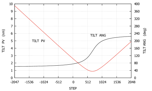
Figure 7: $PV$ and angle of the tilt component of the cavities of Fig. 6 (TILT PV and TILT ANG, respectively), along the full spectral scan. The curves represent the actual values of the parameters derived from the planar fit; both vary very smoothly with $n$. Any local variation of the parameters is contained within the thickness of the font.

As stated above, before the spectral scan we took care to minimize the tilt of the cavity by changing the CS100 parameters, visually controlling the map of cavity errors for the distance corresponding to the central step $n$=0. As shown in Fig. 7, this corresponds to a tilt with $PV\approx$ 2.5 nm, which is probably around the best precision that can be obtained with a visual procedure (cf. discussion in the Introduction). The spectral scan still introduces a significant, additional component that much exceeds the starting value; using the simplified formula of Eq. 2 and the values of Table 1, the extremes of the tilt curve of Fig. 7 would correspond to broadenings of the spectral profiles for this FPI in excess of 100%. This would pose a problem for observing programs that require a large fraction of the full tuning range, for example for the case of broad solar chromospheric lines that are often sampled over several Angstroms (which corresponds to the total wavelength span of a cavity of a few mm gap, in the visible range). In both the classical and telecentric mount, this would, in different ways, result in variations in the instrument profile, creating an increasingly broader and more asymmetric instrumental profile as the scan progresses, away from the optimal, tilt-minimum position. It might also cause the spatial PSF to further vary as a function of wavelength tuning position.

At the same time, we note that the case of Figs. 6 and 7 might represent an extreme situation. As shown in Appendix, we measured the cavity defects of two more ICOS ET50 (on loan from the National Solar Observatory), and in both cases we derive an increase of the tilt when moving to the extremes of the spectral scan. However, the amplitude of the maximum tilt was sensibly smaller than for our case study: for these ET50s we obtained a tilt $PV$ = 0.5 nm for $n$=0, and $PV\approx$ 3 nm at the edge of the scan. Nevertheless, the occurrence of such an effect in multiple similar devices points toward an intrinsic property of these instruments, although we have no direct knowledge of the underlying cause. Since the capacitance bridges should drive the actuators until balanced, it seems plausible that the plates themselves (to which the capacitors are attached) might undergo elastic deformations during the scan.

3.3 Stationary cavity defects

As mentioned above, if we remove the large-scale tilt from the cavity errors map $M(x,y,n)$), we find that the residual shape remains essentially constant throughout the scan, with a residual variation of less than 0.1 nm ($PV$). We can then use any arbitrary scan step to analyze the behavior (and possible cause) of the stationary cavity defects. Figure 8 shows the map $M(x,y,0)$ for the central $n$=0 step, after subtraction of the tilt plane.

We separated the defects at large scale (low spatial frequency) from those at small scale (high frequency) fitting the map of Fig. 8 with the standard 37 Zernike polynomials of the FRINGE subset (Wyant & Creath, 1992). The resulting fits and residuals are shown in Figs. 9 and 10 respectively.

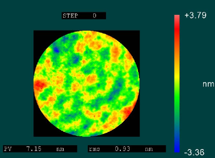
Figure 8: Map $M(x,y,0)$ for the central step of the spectral scan, after removal of the global tilt.

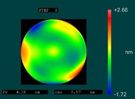
Figure 9: Fit of map $M(x,y,0)$ with the standard 37 Zernike polynomials of the FRINGE subset.

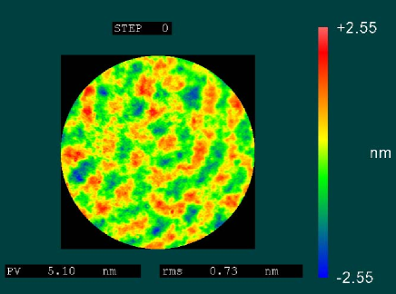
Figure 10: Residuals of M(x,y,0) after removal of tilt and the fit of Fig. 9.

The large scale errors (Fig. 9) describe a cavity with a roughly circular symmetry at the scale of the plates, with peak-to-valley values of 4–5 nm. This appears broadly consistent with the values measured by Reardon & Cavallini (2008, their Figure 10) over the central 35–40 mm of the IBIS’ FPIs, and with the “bowing” effect often observed in systems of this kind, due to the strong surface tension of the coating. The effect, however, is smaller than those introduced by the residual tilt at the extremes of the spectral scan.

We hypothesize that the three yellow and red features (larger cavity gaps) positioned around the perimeter at roughly 120^∘ intervals are due to the local stress imparted by the piezo-electric actuators, that are equally spaced around the plates (see Fig. 11 below). A very similar tri-lobate pattern is measured for the large scale, static cavity errors of one of the NSO FPIs described in Appendix, while for the other we measure a ring-like figure. The bow-shape mentioned above is prominent in one of these two additional FPIs, reaching 2 nm $PV$ (comparable with the tilt measured at the extremes of the spectral scan), while almost negligible in the other. Given that the FPIs are fabricated by the same manufacturer following similar procedures, this highlights how many different factors can determine the final cavity shape, including pre-load stresses applied during assembly of the etalons, and the coating process. Indeed, the cavity shape presented in Fig. 8 of Denker & Tritschler (2005), also obtained by applying the standard Zernike polynomials fit, is different still. However, these authors present a fit to the global cavity, before any large scale defect (such as a tilt) is removed; this can effectively mask subtler effetcts like those displayed in Fig. 9.

The small scale defects (Fig. 10) range within $\pm$ 2.5 nm, again consistently with the results of Reardon & Cavallini (2008). They show a uniform distribution throughout the cavity, with alternating positive and negative regions of average diameter of about 3 mm, probably due to the process of coating deposition (see comments at the beginning of Sect. 3).

4 Dynamic correction of the tilt

As described above, the “spurious” planar tilt in the cavity shape (Fig. 7) introduced by the spectral scan results in significant variations of the instrumental profile. Thus, we attempted to devise a software procedure to minimize the tilt component by actively controlling the plates’ parallelism during the spectral scan, using the ICOS CS100 controllers. To our knowledge, this is the first time that such a correction has been considered for use in an operational instrument based on FPIs.

Figure 11 represents schematically the actuators’ positions, and the capacitance controllers for both separation and parallelism, for the case of the ICOS ET50 etalon. As discussed in Sect. 3.2, once the reference plane is defined, the balancing action of the capacitance bridge should drive properly the piezo-electric actuators and maintain the parallelism for every value of the separation; however, unknown effects partially disrupt this feedback mechanism, with the net result of a varying tilt between the plates. An important characteristics of the CS100 controller however, is the possibility to provide independent values of the x and y tilt components [TILTX, TILTY] to the plates, effectively allowing the user to reset the reference plane at any given spectral step (See e.g., Veilleux et al., 2010, Sect. 3.2, for further description of the CS100’ operation). Exploiting this capability, and having measured the actual cavities at each step as described in Sect. 3.2, we defined a lookup table that associates a pair of (TILTX,TILTY) values to each step $n$ of the scan, so to minimize the overall tilt. The granularity of the (TILTX, TILTY) settings is the same as the step size $\Delta$ ($\sim$ 0.5 nm), allowing a precision in the reference plane of $\Delta_{\theta}\approx 1.4\times 10^{-3}$ (Table 1). The resulting lookup table is given in Fig. 12.

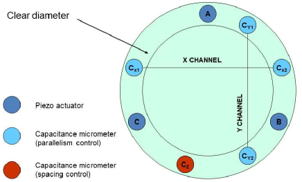
Figure 11: Scheme of the piezo-electric actuators and the capacitance controls for separation and parallelism of the ET50’ plates.

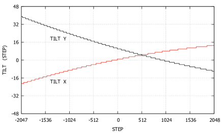
Figure 12: Lookup table of the (TILTX, TILTY) corrections adopted to minimize the cavity tilt introduced by the scan. Each tilt step corresponds to $1.4\dot{1}0^{-3}$ arcsec.

We then again acquired an interferogram at each spectral step, while applying the corrections defined by the lookup table. No extra delay is introduced in the scan, as the software controlling the FPI scan now simply transmits a string of three values: $n_{z}$, $n_{x}=$TILTX$(n_{z})$, and $n_{y}=$TILTY$(n_{z})$, instead of the single $n_{z}$ one. The same fitting procedure described in Sect. 3.2 was applied to the resulting intensity curves, and new maps $M(x,y,n)$ of cavity defects were obtained. Analogously to Fig. 6, Fig. 13 shows the results for the same four different spectral steps after the automated tilt minimization procedure. The animation Fig13.mp4, available in the online version of the paper, shows the resulting map for every spectral step.

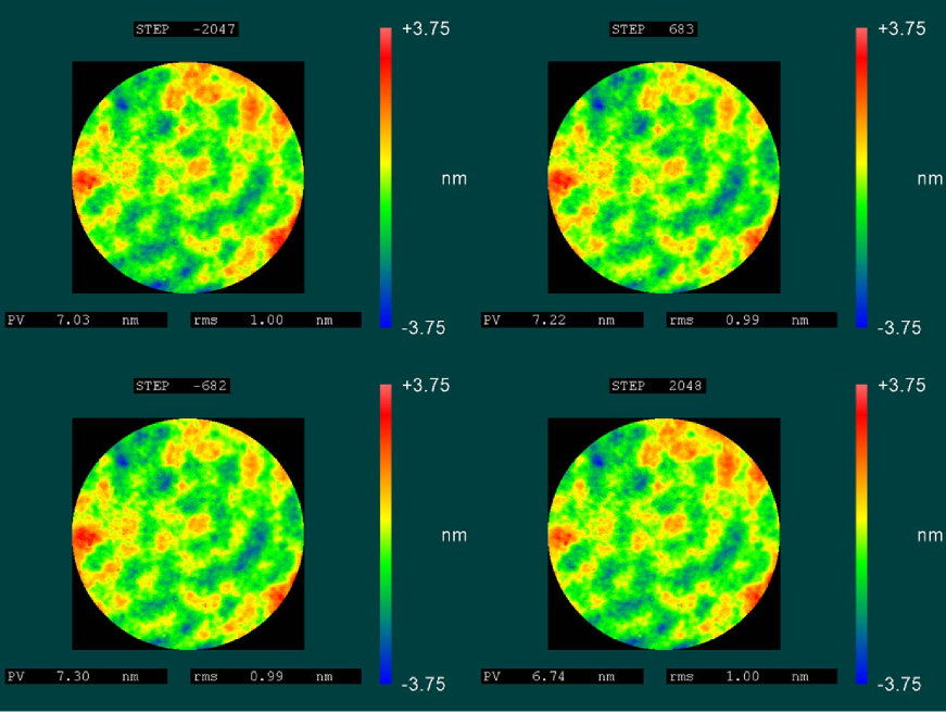
Figure 13: As Fig. 6, but after tilt minimization, as described in the text. The color scale is essentially identical to that of Fig. 8. A movie of the cavity error maps $M^{\prime}(x,y,n)$ for every spectral step is available in the online version of this paper (Fig13.mp4)

The variation of the cavity shape is now strongly reduced; indeed, next we measured a $PV$ and rms value of the cavity defects that vary within

$$\centering 6.7\leavevmode\nobreak\ $nm$\leavevmode\nobreak\ \leq PV\leq 7.3\leavevmode\nobreak\ $nm$;\leavevmode\nobreak\ \leavevmode\nobreak\ \leavevmode\nobreak\ \leavevmode\nobreak\ \leavevmode\nobreak\ 0.980\leavevmode\nobreak\ $nm$\leavevmode\nobreak\ \leq rms\leq 1.0\leavevmode\nobreak\ $nm$,\@add@centering$$ (21)

which are sensibly smaller than the original values of Eq. 20. In particular, by fitting the new cavity defect maps as done in Sect. 3.2 above, we find that the residual tilt after the correction procedure remains smaller than 1 nm, and its direction does not increase monotonically. Rather, after rotating about 150^∘ in the first half of the scan, the sense of rotation is flipped, and the direction returns essentially to the initial value (Fig. 14).

Figure 14: $PV$ and angle of the tilt component of the cavities of Fig. 13 (TILT PV and TILT ANG, respectively), along the full spectral scan. The curves represent the actual values of the parameters derived from the planar fit; both vary very smoothly with $n$. The tilt $PV$ remains within the 1 nm value.

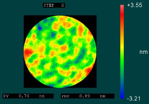
Figure 15: Cavity defects map $M(x,y,0)$ obtained applying the tilt minimization technique described in the text four months after deriving the corrective lookup table.

In order to estimate how reliable and reproducible the correction technique is (and hence the stability of the system), we repeated the same measures after an interval of four months, using the same initial settings of the CS100, and the same lookup table of Fig. 12. Fig. 15 shows the resulting cavity defects map $M(x,y,0)$ at the central $n$=0 step. The derived map is essentially identical to that of Fig. 8, testifying to the stability of the system and the reproducibility of the correction. The $PV$ value of the tilt (not shown) remains below 1 nm. A long-term stability of the parallelism of the plates has been noted earlier by Veilleux et al. (2010), that comment how the same tilt parameters could be applied from run to run over a period of years. This agrees with our experience in operating IBIS at the Dunn Solar Telescope over fifteen years.

As a final note, we also highlight how the technique described by Eqs. 12 – 15 is sensitive enough to measure the cavity variations due to deformation of the optical surfaces during the scan. This was one of our original goals, as discussed in the Introduction. In Fig. 16 we show the difference maps $M(x,y,n)-M(x,y,0)$ for four different values of $n$ ($n$=$-$2047,$-$682,$+$683,$+$2048), after removal of the tilt component. The scale of variation is much smaller than that due to the tilt (about one order of magnitude), but still significant, and with some definite spatial structure. For example, it is interesting to note how, during a scan, the piezo-electric actuators introduce a small astigmatism that rotates about 90^∘ from one extreme to the other.

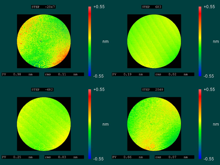
Figure 16: Cavity variations due to the deformation of the optical surfaces during a scan. The maps have been obtained by subtracting $M(x,y,0)$ from $M(x,y,n)$, after removal of the tilt. The small-scale fringes and straight patterns are due to residual interference between the optical surfaces, and from the CCD readout, respectively, and are not related to the shape of the cavity.

5 Discussion and conclusions

In this paper we have introduced a new technique to precisely measure the cavity defects of Fabry-Perot interferometers, which represent the core components of a large variety of astronomical instruments, both for nighttime and solar studies. The exact knowledge of the cavity is a necessary step to properly understanding an instrument’s performance (shape and variation of the instrumental profile) and interpret the observations.

Our method, based on Eqs. 12-15, is an extension of the phase-shifting techniques developed to characterize optical surfaces (Schreiber & Bruning, 2007) and can be applied to FPIs with any value of the reflectivity R. The method can be used by measuring either the transmission or reflection interference pattern (Sect. 2.2); the latter is however more versatile, as it could be used also for the case of uncoated cavities, or for wavelengths for which R is low. We envision, for example, using the same setup described in this paper (with a HeNe laser) to characterize cavities coated for near-infrared observations.

The measures were performed at the Italian Istituto Nazionale di Ottica. Our setup, depicted in Fig. 2, was realized using a phase-shifting interferometer GPI-XP of Zygo-Ametek (www.zygo.com), that outputs a collimated HeNe ($\lambda$=632.8 nm) laser beam of 100 mm diameter. In a future work, we plan to employ an existing 150 mm laser beam expander to extend this study to FPIs of larger diameter.

Similarly to the work described by Denker & Tritschler (2005) and Reardon & Cavallini (2008), we used measurements of the reflected (transmitted) intensity from the HeNe laser to derive the cavity shape of an FPI mounted in a collimated configuration. As an extension of these works, however, we explicitly considered the possibility that the cavity shape can change during the spectral scan. We employed our technique to fully characterize the cavity of three separate ET50 interferometers (50 mm in diameter, coated for use in the visible range), all fabricated by ICOS Ltd.

Our most important result is that the cavity shape does indeed change significantly during a full spectral scan. Even after the “standard” alignment procedure, of the kind usually employed during instrumental setup at the telescope, a significant residual tilt is observed, that smoothly increases toward the edges of the scan. The effects of this residual tilt on the overall transmission profile can be severe: as shown in Sect. 3.2, in our worst example they can result in a doubling of the FWHM of the instrumental profile, depending on the position within the scan. We remark, however, that the effects appear substantially milder for the other two FPIs tested, which are of more recent fabrication and which, we hypothesize, might have a more uniform coating. Still, tests to characterize the cavity shape at each spectral step should be performed in order to properly characterize any given instrument.

To our knowledge this is the first time that this spectral dependence of the cavity shape is characterized. Interestingly, Veilleux et al. (2010) reported a broad dependence of the tilt on the spacing for the case of the MMTF, but at a much coarser spectral resolution (i.e., $z$-axis settings of the CS100). Further, their results might also be affected by the dependence of the cavity shape on wavelength (see discussion below).

The variation pattern of the measured tilt (Figs. 6 and 7) appears consistent with an over- (or under-) correction of one of the actuators with respect to the other two, maybe because of an elastic deformation of the plates to which the capacitive sensors are attached. As the same qualitative behavior is observed for all the three ICOS ET50 tested, this points toward an intrinsic operational characteristics of these systems. Preliminary tests with a larger-format, uncoated interferometer also reveal a similar pattern, supporting our findings (Greco et al, in prep.).

To minimize the residual tilt during the scan, we devised a correction procedure that exploits the capabilities of the CS100 controller to dynamically input a value for the the tilts of both the $x$ and $y$ axes for each step of the spectral scan ($z$ axis). After applying the measuring technique described above, and fitting a planar tilt to the cavity shape at each spectral step, we derive a lookup table of the additional (TILTX,TILTY) values necessary to minimize the tilt component for every step. The commands can be provided within the same controlling sequence used for the spectral scan, without introducing any additional delay. The results are highly encouraging, with the corrective sequence limiting the residual tilt to $PV$ values of less than 1 nm. Moreover, the system appears very stable: the same results were obtained when applying the initial settings, and the lookup table described above, after a long period (four months). Together with the very slow dependence of the tilt on the step number $n$, this extreme repeatability points toward an elastic deformation of the cavity as mentioned above. The stability of ICOS FPI systems in terms of their setup parameters in operational situations has indeed been reported numerous times (e.g., Veilleux et al., 2010); this holds promise that our corrective procedure can be effectively adopted for existing and future instrumentation.

Once the variable terms were taken into account, it was possible to uncover the “static” cavity shape, resulting from the overall fabrication process. This appears to be a combination of two main components: a large-scale one, showing both a bow shape, typical of the strong surface tension of the coating and a tri-lobate figure most likely due to the local stresses introduced by the piezo actuators, positioned at 120^∘ from one another; and a small scale component (of size one to a few mm on the plates) probably due to the coating deposition process. The overall deviations from cavity flatness are significant enough to make it necessary to account for them in the calculation of the overall instrumental profile (Reardon & Cavallini, 2008). A different optical figure is however obtained for one of the three ET50 analyzed, probably due to differential contributions of the many factors entering the fabrication and assembly of the etalons; this reinforces the need to obtain an exact measurement of each interferometer cavity to properly evaluate the instrumental transmission profile.

All of the results presented above have been obtained using a monochromatic HeNe laser at 632.8 nm, leaving open the question of whether they would hold at different wavelengths. Indeed, several instances have been reported in the literature of operational FPI systems for nighttime astronomy where the tilt optimal values were strongly wavelength dependent (Rangwala et al., 2008; Veilleux et al., 2010; González et al., 2014). However, as already discussed by Jones & Bland-Hawthorn (1998) in their analysis of the TTF, this effect is mainly observed for etalons with very small gaps (few to tens of $\mu$m), which are comparable to the thickness of the optical coatings.

Wavelength-dependent phase changes and non-uniformities should be less important at the large gaps usually employed in instruments for solar physics. It is, however, worth noting that a recent study of the coatings of VTF (Pinard et al., 2018) mentions the possibility that phase differences at different laser wavelengths might exist. We plan to study these effects in a future work by implementing the same optical setup, but with different laser sources. If tilt variations are a manifestation of true changes in physical plate separation, then we expect that this effect will manifest itself, additively, together with the other wavelength dependent sources of effective plate separation.

Appendix A The cavity errors of additional ET50 interferometers

To test our procedure on different etalons, we used two additional ICOS ET50 interferometers obtained on loan from NSO. The etalons have been fabricated in the mid 1990s, with cavity spacings of 2.8 mm and 609 $\mu$m respectively. Other relevant instrumental characteristics are comparable to those reported in Table 1; in particular the operational wavelength range is 400–700 nm as well, with a coating reflectivity of about 95%.

For both ET50, we measured the reflected interferograms over a full spectral scan, as described in Section 3. The resulting images were analyzed by fitting the fringe pattern in each pixel’s intensity curve with Eq. 13. The resulting cavity errors at four different spectral steps are represented in Figs. 17 and 18 for the two FPIs, in the same way shown in Fig. 6 for the interferometer studied in the main body of the paper.

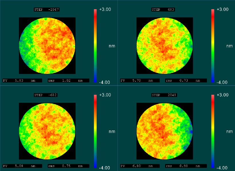
Figure 17: As Fig. 6, for the 609 $\mu$m gap NSO ET50.

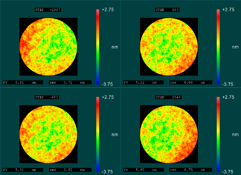
Figure 18: As Fig. 6, for the 2.8 mm gap NSO ET50.

The results are consistent with what we report in Sect. 3.2. First of all, the $PV$ and $rms$ of the cavity errors vary sensibly within the spectral scan, with $PV$ values between 5 and 6.8 nm, and $rms$ values between 0.7 and 1 nm for the first NSO etalon; and $PV$ between 5.1 and 6.4 nm, and $rms$ between 0.62 and 0.75 nm for the second one. Further, an obvious tilt component is visible in the cavity errors maps of both Figs. 17 and 18; its evolution within the spectral scan essentially causes the variation of the $PV$ values described above. As described in Sec. 3.2, we then fit a plane to the error maps derived at each spectral step; the resulting parameters of the plane (tilt $PV$ value and angle) are displayed in Figs. 19 and 20.

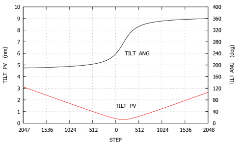
Figure 19: $PV$ and angle of the tilt component of the cavity error maps of the 609 $\mu$m gap NSO ET50 (Fig. 17).

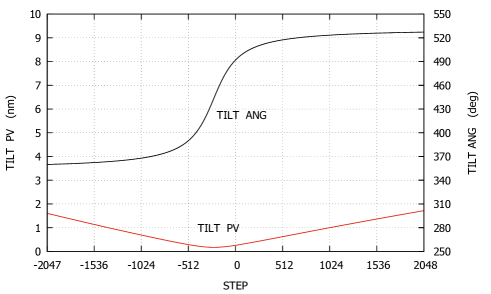
Figure 20: As Fig. 19 for the 2.8 mm gap ET50 of NSO (Fig. 18).

The curves are qualitatively similar to those shown in Fig. 7, meaning that the tilt reaches a minimum value around the middle of the spectral scan (where initial parallelism is set), and increases monotonically toward the edges. The tilt angle flips sign around the minimum of the tilt $PV$ value, consistently with the idea expressed above of an over- or under- correction by the piezo-actuators in a given direction. The amplitude of the changes is however much smaller than for the IPM etalon. Still, as we describe in the Introduction, with the typical values of reflectivity and working wavelength for these instruments, a residual $PV$ tilt value around 3 nm corresponds to a substantial broadening of the transmission profile.

Here we do not show the subsequent elaborations (removal of the tilt, analysis of the static defects etc.) but they are fully consistent with what shown for the IPM etalon in the body of the paper. Worth noting is the different spatial size of the residual static defects, appreciable already in Figs. 17 and 18. These are most likely due to variations in the coating substrate among the different interferometers and coating runs.