GPU accelerated fast multipole boundary element method for simulation of 3D bubble dynamics in potential flow

Abstract

A numerical method for simulation of bubble dynamics in three-dimensional potential flows is presented. The approach is based on the boundary element method for the Laplace equation accelerated via the fast multipole method implemented on a heterogeneous CPU/GPU architecture. For mesh stabilization, a new smoothing technique using a surface filter is presented. This technique relies on spherical harmonics expansion of surface functions for bubbles topologically equivalent to a sphere (or Fourier series for toroidal bubbles). The method is validated by comparisons with solutions available in the literature and convergence studies for bubbles in acoustic fields. The accuracy and performance of the algorithm are discussed. It is demonstrated that the approach enables simulation of dynamics of bubble clusters with thousands of bubbles and millions of boundary elements on contemporary personal workstations. The algorithm is scalable and can be extended to larger systems.

1 Introduction

Bubbles are common in nature and in many technological processes Brennen1995 including surface cleaning by ultrasound Xi2012 and biomedical applications Ovenden2017 . Very complex physics of gas-liquid systems may govern the bubble dynamics since at different conditions different effects can be dominating (e.g., Nigmatulin1991 ). So, it is not surprising that most of studies related to single bubble dynamics or bubbly liquids, where such effects should be taken into account, treat bubbles as spherical objects (e.g., Plesset1977 ; Akhatov1997 ; Khabeev2009 ; Lauterborn2010 ; Parlitz1999 ; Gumerov2012 ). Simulations of bubble dynamics of arbitrary shape are usually performed using simpler models, such as the model of incompressible inviscid liquid and a spatially uniform polytropic gas. In this case, boundary element methods (BEM) are among the most efficient approaches since they require only boundary discretization, which can be done using a substantially smaller number of elements compared to the methods based on volume discretization to achieve the same accuracy.

The BEM for two-dimensional (or axisymmetric) dynamics of a single bubble near a solid wall and a free surface was developed and used successfully by many researchers Voinov1975 ; Blake1987 ; Best1992 ; Boulton-Stone1993A ; Boulton-Stone1993B ; Oguz1990 ; Oguz1993 . In these references also comparisons with experimental data can be found. A three-dimensional boundary element method was applied to study the dynamics of bubbles arising from an underwater explosion or induced by a laser or a spark (e.g.,Chahine1992 ; Chahine1994 ; Zhang1993 ; Zhang2001 ). The BEM was used for determination of the bubble shape Gumerov2000 , investigation of bubble self-propulsion in potential flows Itkulova2014 , energy dissipation during bubble collapse Lee2007 , and bubble dynamics in Stokes flows Pozrikidis2003 ; Itkulova2013 .

Note that large-scale three-dimensional problems are computationally complex and resource-intensive. Certainly, there is no way to simulate multiphase flows consisting of billions of bubbles directly, and either continuum approaches or various schemes coupling micro-,
mezo-, and macroscales can be found in the literature. However, bubble clusters consisting of hundreds or thousands bubbles may not be well described by continuum theories or simplified theories neglecting bubble shape effects. Capabilities for computation of dynamics of such systems can be important for validation of multiscale approaches and study of various effects in mezoscales. So the development of methods for acceleration of direct simulations is critical and such attempts can be found in the literature (e.g., Bui2006 ).

The approach of the present work relies on the BEM accelerated both via a scalable algorithm, namely, the fast multipole method (FMM), and utilization of advanced hardware, namely, graphics processors (GPUs) and multicore CPUs. The primary computational challenge of the classical BEM is related to solving of a large dense system of $N$ algebraic equations for each time step, where $N=MN_{d}$ is the total number of collocation points, $M$ is the number of bubbles, $N_{d}$ is the number of the collocation points on a single bubble surface. Indeed, in this case, the cost of the direct solution is $O\left(N^{3}\right)$. This cost can be reduced to $O\left(N_{iter}C_{MVP}\right)$ using the iterative methods, where $N_{iter}\ll N$ is the number of iterations, and $C_{MVP}$ is the cost of the matrix-vector product (MVP). If performed directly the latter value can be estimated as $O\left(N^{2}\right)$. The application of the FMM reduces the complexity of MVP operation to $O(N)$, which results in the total cost of the method $O\left(N_{iter}N\right)$.

The FMM was introduced by Rokhlin and Greengard Greengard1987 and further developed by these and other researchers (particularly, for the Laplace equation in three dimensions, e.g., Cheng1999 ; Gumerov2008 ). Comparison of efficiency of different methods for the Laplace equation in 3D can be found GumerovL2005 . A number of authors considered acceleration of the BEM using the FMM (e.g., Nishimura2002 ; Gumerov2006 ; Liu2009 ). The BEM accelerated via the FFTM (an FMM-type scalable algorithm combining the single level FMM and the FFT) was successfully used for bubble dynamics simulations by Bui et al Bui2006 . While both the FMM and the FFTM have $O\left(N\right)$ or $O\left(N\log N\right)$ complexity, the difference can appear in simulations of large systems as the FMM may be more efficient for highly non-uniform distributions, where skipping of empty boxes can be essential.

The FMM can be efficiently parallelized Greengard1990 . The first implementation of the FMM on graphics processors Gumerov2008 was developed further Hu2011 ; Hu2012 , where the FMM was implemented on heterogeneous computing architectures consisting of multicore CPUs and GPUs. This FMM parallelization strategy for heterogeneous architectures was successfully used in fluid and molecular dynamics Itkulova2012 ; Abramova2013 ; Abramova2014 ; Hu2013 ; Maryin2013 and in electro- and magnetostatics Adelman2017 . A similar approach is applied in the present study for simulation of bubble dynamics with millions of boundary elements on personal workstations. It should be mentioned that there exist different FMM parallelization strategies for heterogeneous architectures and demonstrations of high-performance applications for simulation of blood flows, turbulence, etc. (e.g., Lashuk2009 ; Rahimian2010 ; Yokota2013 ).

It is well known that BEM-based bubble dynamics codes cannot work correctly without mesh stabilization and smoothing (e.g., Zhang2001 , also some literature review can be found here). Indeed, smooth bubble surface is provided naturally by surface tension and liquid viscosity and compressibility. In many cases, the spatial and temporal scales related to these effects are much smaller compared to the characteristic scales of bubble dynamics (e.g., the frequency of oscillations and the bubble size). To achieve natural (physical) smoothing substantially small time steps and fine surface meshes should be employed. In simplified models, where either all these effects are neglected (e.g., Bui2006 ), or they have taken into account only partially (e.g., just the surface tension) artificial stabilization and smoothing of the surface should be used. A similar situation can be observed, e.g., in the modeling of shock waves, where the viscosity provides an extremely thin boundary layer, while for simulation of shock waves in inviscid media various methods are used to stabilize computations. In the present study, we propose a novel technique for smoothing based on shape filters. We also provide details necessary for development and implementation of a stable and efficient bubble dynamics code.

The goal of this paper is to present the method and show its performance and scaling with the problem size. For this purpose, we used several benchmark problems. To validate the code and compare with the data available in the literature we used small-scale examples (several bubbles). The performance and scaling are studied on a somewhat artificial configuration of a “regular” bubble cluster. The reason for this is that such clusters can be easily reproduced by other researchers and they can use the data provided in this paper for comparisons and validations. It should be noticed that the code can compute the dynamics of bubbles of different topology, including toroidal bubbles (and the reader can find expressions for the toroidal shape filter). However, the description for the handling of the topology change and peculiarities of such modeling (which can be found elsewhere) brings unnecessary complication to the presentation and does not contribute to the demonstration of the performance of the method, which is the main goal. So, for the clarity of presentation, we limited ourselves with examples for bubbles topologically equivalent to a sphere. The authors also expect future publications with more physically interesting cases simulated using the method presented in this paper.

2 Statement of the problem

2.1 Governing equations

Consider the dynamics of a cluster consisting of $M$ gas bubbles in an incompressible inviscid liquid of density $\rho$, which motion is described by equations

$$\rho\frac{d\mathbf{v}}{dt}=-\nabla p+\rho\mathbf{g},\quad\nabla\cdot\mathbf{v}=0,\quad\frac{d}{dt}=\frac{\partial}{\partial t}+\mathbf{v}\cdot\nabla,$$ (1)

where $\mathbf{v}$ is the liquid velocity, $p$ the pressure, and $\mathbf{g}$ the gravity acceleration. These equations have a solution in the form of potential flow,

$$\mathbf{v}=\nabla\phi,$$ (2)

where $\phi$ is the velocity potential satisfying the Laplace equation at any moment of time,

$$\nabla^{2}\phi\left(\mathbf{r},t\right)=0.$$ (3)

Spatial integration of Eq. (1) results in the Cauchy-Lagrange (unsteady Bernoulli) integral,

$$\frac{\partial\phi}{\partial t}+\frac{1}{2}\left|\nabla\phi\right|^{2}+\frac{p}{\rho}=\mathbf{g\cdot r}+F(t),$$ (4)

where $F(t)$ is the integration constant, which should be determined from the boundary conditions at the infinity. For liquid resting far from the bubble at pressure $p_{\infty}(t)$, we have

$$\left.\phi\right|_{\left|\mathbf{r}\right|\rightarrow\infty}=0,\quad\left.p\right|_{\left|\mathbf{r}\right|\rightarrow\infty}=p_{\infty}\left(t\right)+\rho\mathbf{g\cdot r,\quad}$$ (5)

$$F\left(t\right)=p_{\infty}\left(t\right)/\rho.$$

Notably, for time-harmonic acoustic fields considered in this study, $p_{\infty}(t)$ is specified as

$$p_{\infty}(t)=p_{0}+p_{a}(t),\quad p_{a}(t)=-P_{a}\sin\omega t,$$ (6)

where $p_{0}$ is the static pressure and $p_{a}(t)$ is the acoustic pressure characterized by the amplitude $P_{a}$ and the circular frequency $\omega$.

The total gas-liquid interface $S$ is a union of interfaces of all bubbles, $S=S_{1}\cup...\cup S_{M}$, where $S_{m}$ is the surface of the $m$th bubble, $m=1,...,M.$ The liquid pressure $p(\mathbf{r},t)$ and the gas pressure, $p_{gm}\left(t\right)$, on the bubble surface $S_{m}$ are related as

$$p\left(\mathbf{r,}t\right)=p_{gm}\left(t\right)-2\sigma H_{m}\left(\mathbf{r,}t\right),$$ (7)

$$\mathbf{r}\in S_{m},\quad m=1,...,M,$$

where $\sigma$ is the surface tension and $H_{m}\left(\mathbf{r,}t\right)$ is the mean surface curvature. The gas pressure depends on the bubble volume according to the polytropic law,

$$p_{gm}\left(t\right)=p_{gm0}\left(\frac{V_{m0}}{V_{m}}\right)^{\kappa},$$ (8)

$$p_{gm0}=p_{0}+\frac{2\sigma}{a_{m0}},\quad m=1,...,M,$$

where $\kappa$ is the polytropic exponent (for the isothermal processes $\kappa=1$ and for the adiabatic processes $\kappa=\gamma_{g}$, where $\gamma_{g}$ is the gas specific heats ratio), subscript “0” refers to the initial value at $t=0$, $V_{m}$ is the $m$th bubble volume, and $a_{m0}$ is the effective bubble radius at $t=0$ (assuming that the hydrostatic pressure gradient has a negligible effect on the initial bubble shape).

Evolution of the velocity potential and the gas-liquid interface is determined by the dynamic and kinematic conditions,

$$\frac{d\phi}{dt}=\frac{1}{2}\left|\mathbf{v}(\mathbf{r,}t)\right|^{2}-\frac{p_{gm}\left(t\right)-2\sigma H_{m}\left(\mathbf{r,}t\right)}{\rho}$$

$$+\mathbf{g\cdot r}+F(t),\quad\mathbf{r}\in S_{m},\quad m=1,...,M,$$

$$\frac{d\mathbf{r}}{dt}=\mathbf{v}(\mathbf{r,}t),\quad\mathbf{n}\cdot\mathbf{v}=\frac{\partial\phi}{\partial n}=q,\quad\mathbf{r}\in S,$$ (10)

where $\mathbf{n}(\mathbf{r,}t)$ is the normal to the surface $S$. These relations close the problem. Indeed, Eq. (10) propagates the boundary value of the potential to the next time step. The potential also determines the tangential velocity as the derivative of this quantity along the surface. The normal component of the velocity can be found from the solution of the Dirichlet boundary value problem for the Laplace equation. As soon as the surface velocity is found the position of the interface can be updated.

2.2 Boundary integral equations

The BEM uses a formulation in terms of boundary integral equations (BIE) whose solution with boundary conditions provides $\phi(\mathbf{r})$ and $q(\mathbf{r})=\partial\phi(\mathbf{r})/\partial n(\mathbf{r})$ on the boundary and subsequently determines $\phi(\mathbf{r})$ for external and boundary domain point $\mathbf{r}$. Using Green’s identity the boundary integral equations for $\phi|_{|\mathbf{r}|\rightarrow\infty}=0$ can be written in the form

$$L\left[q\right]\left(\mathbf{r}\right)-M\left[\phi\right]\left(\mathbf{r}\right)=\left\{\begin{array}[]{c}-\phi\left(\mathbf{r}\right),\quad\mathbf{r}\notin S,\quad\mathbf{r}\in\Omega,\\ -\frac{1}{2}\phi\left(\mathbf{r}\right),\quad\mathbf{r}\in S,\\ 0,\quad\mathbf{r}\notin\Omega.\end{array}\right.$$ (14)

Here $\Omega$ is the domain occupied by liquid, and $L[q]$ and $M[\phi]$ are the single and double layer potentials, respectively:

$$L\left[q\right]\left(\mathbf{r}\right)=\int_{S}q\left(\mathbf{r}^{\prime}\right)G\left(\mathbf{r},\mathbf{r}^{\prime}\right)dS(\mathbf{r}^{\prime}),$$ (15)

$$M\left[\phi\right]\left(\mathbf{r}\right)=\int_{S}\phi\left(\mathbf{r}\right)\frac{\partial G\left(\mathbf{r},\mathbf{r}^{\prime}\right)}{\partial n\left(\mathbf{r}^{\prime}\right)}dS(\mathbf{r}^{\prime}),$$

where $G\left(\mathbf{r},\mathbf{r}^{\prime}\right)$ is the free space Green’s function for the Laplace equation, and $\partial G\left(\mathbf{r},\mathbf{r}^{\prime}\right)/\partial n\left(\mathbf{r}^{\prime}\right)$ is its normal derivative for the normal directed outside the bubble

$$G\left(\mathbf{r},\mathbf{r}^{\prime}\right)=\frac{1}{4\pi\left|\mathbf{r}-\mathbf{r}^{\prime}\right|},$$ (16)

$$\frac{\partial G\left(\mathbf{r},\mathbf{r}^{\prime}\right)}{\partial n\left(\mathbf{r}^{\prime}\right)}=\frac{\mathbf{n}\left(\mathbf{r}^{\prime}\right)\cdot\left(\mathbf{r}-\mathbf{r}^{\prime}\right)}{4\pi\left|\mathbf{r}-\mathbf{r}^{\prime}\right|^{3}}.$$

3 Numerical method

3.1 Discretization

Discretization of the boundary results in an approximation of surface functions via finite vectors of their surface samples and integral operators via matrices acting on that vectors. In the present study, the surface $S$ is discretized by a triangular mesh with $N$ vertices $\mathbf{r}_{i}$, $i=1,...,N$, which used as the collocation points. For a given set of collocation points, the quadratures for the single and double layer integrals can be written in the form

$$L\left[q\right]\left(\mathbf{r}_{i}\right)\approx\sum_{j=1}^{N}L_{lj}q_{j},\quad M\left[\phi\right]\left(\mathbf{r}_{i}\right)\approx\sum_{j=1}^{N}M_{ij}\phi_{j},$$ (17)

$$\phi_{j}=\phi\left(\mathbf{r}_{j}\right),\quad q_{j}=q\left(\mathbf{r}_{j}\right),$$

where $L_{ij}$ and $M_{ij}$ are the elements of the BEM $N\times N$ matrices $\mathbf{L}$ and $\mathbf{M}$ representing the surface operators. They can be found by evaluation of the integrals over the triangles sharing a given collocation point $\mathbf{r}_{j}$. Discretization (17) of the boundary integral equation (14) results in a linear system

$$\sum_{j=1}^{N}L_{ij}q_{j}=b_{i},\quad b_{i}=-\frac{1}{2}\phi_{i}+\sum_{j=1}^{N}M_{ij}\phi_{j},$$ (18)

$$i=1,...,N,$$

which can also be written in the matrix-vector form

$$\mathbf{Lq}=\mathbf{b,\quad b=}-\frac{1}{2}\boldsymbol{\phi}+\mathbf{M}\boldsymbol{\phi},\quad$$ (19)

$$\mathbf{L}=\left\{L_{ij}\right\},\quad\mathbf{M}=\left\{M_{ij}\right\},$$

$$\mathbf{q}=\left\{q_{j}\right\},\quad\mathbf{b}=\left\{b_{i}\right\},\quad\boldsymbol{\phi=}\left\{\phi_{i}\right\}.\quad$$

3.2 Non-singular integrals

There exist extensive literature for accurate numerical and analytical evaluation of the integrals of the Green’s function and its derivatives over triangles (e.g., Chen02 ; Adelman2016 ). However, efficient use of the FMM for large $N$ requires numerically inexpensive quadratures and approximations, which brings forward strategies, such as described Gumerov2009 . This scheme is used in the present study for computation of the non-singular elements,

$$L_{ij}=s_{j}G\left(\mathbf{r}_{i},\mathbf{r}_{j}\right),\quad M_{ij}=s_{j}\frac{\partial G}{\partial n_{j}}\left(\mathbf{r}_{i},\mathbf{r}_{j}\right),\quad i\neq j,$$ (20)

$$s_{j}=\frac{1}{3}\sum_{S_{k}\ni\mathbf{r}_{j}}A_{k},\quad\mathbf{n}_{j}=\frac{\mathbf{m}_{j}}{\left|\mathbf{m}_{j}\right|},\quad\mathbf{m}_{j}=\sum_{S_{k}\ni\mathbf{r}_{j}}\mathbf{N}_{k}A_{k},$$

where $s_{j}$ and $\mathbf{n}_{j}$ are the surface area (weight) and the unit normal associated with the $j$th vertex, and the summation is taken over all triangles $S_{k}$ of area $A_{k}$ and normal $\mathbf{N}_{k}$ sharing the vertex. This scheme was compared with higher order quadratures Gumerov2009 and tested on large scale problems for the Helmholtz equation. It showed good results for “good” meshes (a “good” mesh consists of “good” triangles of approximately the same size; the goodness of a triangle is characterized by its deviation from a “perfect” triangle, which is an equilateral triangle).

3.3 Singular integrals

Singular integrals can be computed based on the integral identities, which provide expressions for these integrals via the sums of the regular integrals over the surface. The identities can be derived from Green’s identities applied to analytical solutions of the test problems. Such methods were developed and tested for the Laplace and Helmholtz equations and used by several authors (e.g., Gumerov2009 ; Klaseboer2009 ). The method used in the present study is the following.

A test function $\Phi$, which is harmonic and regular inside the interior of domain $\mathbb{R}^{3}\backslash\Omega$ (inside the bubbles), satisfies the identity

$$\frac{1}{2}\Phi\left(\mathbf{r}\right)=L\left[Q\right]\left(\mathbf{r}\right)-M\left[\Phi\right]\left(\mathbf{r}\right),\quad\mathbf{r}\in S,$$ (21)

$$Q=\frac{\partial\Phi}{\partial n}.$$

A discrete form of this relation can be written as

$$L_{ii}Q_{i}=\sum_{j\neq i}\left(M_{ij}\Phi_{j}-L_{ij}Q_{j}\right)+\left(\frac{1}{2}+M_{ii}\right)\Phi_{i},$$ (22)

$$i=1,...,N.$$

First, we determine the diagonal elements of matrix $\mathbf{M}$. A non-trivial regular harmonic function can be taken as $\Phi\left(\mathbf{r}\right)\equiv 1$, for which $Q=0$. So requesting that this solution is exact for the discrete form, i.e., setting $\Phi_{i}=1$ and $Q_{i}=0$ in Eq. (22), we obtain

$$M_{ii}=-\frac{1}{2}-\sum_{j\neq i}M_{ij},\quad i=1,...,N.$$

To determine the singular elements of matrix $L$ we use three test functions $\Phi_{1}\left(\mathbf{r}\right)\equiv x,$ $\Phi_{2}\left(\mathbf{r}\right)\equiv y,$ $\Phi_{3}\left(\mathbf{r}\right)\equiv z$, which normal derivatives on the surface are the components of the normal vector $\mathbf{n=}\left(n_{x},n_{y},n_{z}\right)$, i.e., $Q_{1}\left(\mathbf{r}\right)\equiv n_{x}\left(\mathbf{r}\right),$ $Q_{2}\left(\mathbf{r}\right)\equiv n_{y}\left(\mathbf{r}\right),$ $Q_{3}\left(\mathbf{r}\right)\equiv n_{z}\left(\mathbf{r}\right)$. Note then that Eq. (22) can be written in the vector form,

$$L_{ii}\mathbf{n}_{i}=\sum_{j\neq i}\left(M_{ij}\mathbf{r}_{j}-L_{ij}\mathbf{n}_{j}\right)+\left(\frac{1}{2}+M_{ii}\right)\mathbf{r}_{i},$$ (23)

$$i=1,...,N.$$

Taking the scalar product of this relation with $\mathbf{n}_{i}$ for each collocation point, we obtain

$$L_{ii}=\mathbf{n}_{i}\left[\sum_{j\neq i}\left(M_{ij}\mathbf{r}_{j}-L_{ij}\mathbf{n}_{j}\right)+\left(\frac{1}{2}+M_{ii}\right)\mathbf{r}_{i}\right],$$ (24)

$$i=1,...,N.$$

The computational cost of the above procedure when using the FMM is equal to the cost of four FMM function calls (one for the diagonal of $\mathbf{M}$ matrix and three for the diagonal of $\mathbf{L}$ matrix) since a single call of the FMM can handle input as a sum of monopoles and dipoles. As it is mentioned below, the number of the FMM calls per time step can be several times larger. Hence, the method described is consistent with the overall algorithm complexity. However, it may create 20-30% overhead for an FMM-based linear system solver and more efficient methods can be developed in future.

3.4 Tangential velocity

Determination of the full velocity $\mathbf{v}$ for potential flow is needed for computation of the pressure and time evolution of the surface potential (see Eqs (2.1) and (10)). In the present study, we implemented the following method of surface differentiation consistent with the low order BEM (constant panel or linear approximations).

The velocity on the surface can be decomposed into its normal and tangential components,

$$\mathbf{v=n}q+\mathbf{v}_{t},\quad\mathbf{v}_{t}=\left(\mathbf{n}\times\mathbf{v}\right)\times\mathbf{n}.$$ (25)

To obtain $\mathbf{n}\times\mathbf{v}$ we use the Stokes theorem in the form

$$\int_{S_{k}}\left(\mathbf{n}\times\mathbf{v}\right)dS=\int_{C_{k}}\phi\left(\mathbf{r}\right)d\mathbf{r,\quad v}=\nabla\phi,$$ (26)

where $S_{k}$ is the $k$th surface triangle and $C_{k}$ is the contour bounding $S_{k}$. Assume that the triangle has positive orientation for the path $\mathbf{r}_{k1}\rightarrow\mathbf{r}_{k2}\rightarrow\mathbf{r}_{k3}\rightarrow\mathbf{r}_{k1}$ connecting the respective triangle vertices. At these vertices, the values of $\phi$ are known and can be denoted as $\phi_{k1},\phi_{k2},$ and $\phi_{k3}$, respectively. The linear interpolation along the segment $C_{kij}$ connecting $\mathbf{r}_{ki}$ and $\mathbf{r}_{kj}$ can be written in the form

$$\phi\left(\mathbf{r}\right)=\left(1-\xi\right)\phi_{ki}+\xi\phi_{kj},$$ (27)

$$\mathbf{r}=\left(1-\xi\right)\mathbf{r}_{ki}+\xi\mathbf{r}_{kj},\quad\xi\in\left[0,1\right],\quad i,j=1,2,3.$$

Hence, we have for the line integral along $C_{kij}$

$$\mathbf{I}_{kij}=\int_{C_{kij}}\phi(\mathbf{r})d\mathbf{r}$$ (28)

$$=\left(\mathbf{r}_{kj}-\mathbf{r}_{ki}\right)\int_{0}^{1}\left[\left(1-\xi\right)\phi_{ki}+\xi\phi_{kj}\right]d\xi$$

$$=\frac{1}{2}\left(\mathbf{r}_{kj}-\mathbf{r}_{ki}\right)\left(\phi_{ki}+\phi_{kj}\right).$$

The surface average value of vector $\mathbf{n}\times\mathbf{v}$ over the triangle $S_{k}$ can be computed according to Eqs (25) and (28),

$$\left(\mathbf{n}\times\mathbf{v}\right)_{k}=\frac{1}{A_{k}}\int_{S_{k}}\left(\mathbf{n}\times\mathbf{v}\right)dS$$ (29)

$$=\frac{1}{A_{k}}\left(\mathbf{I}_{k12}+\mathbf{I}_{k23}+\mathbf{I}_{k31}\right)$$

$$=\frac{1}{2A_{k}}\left[\left(\mathbf{r}_{k2}-\mathbf{r}_{k3}\right)\phi_{k1}+\left(\mathbf{r}_{k3}-\mathbf{r}_{k1}\right)\phi_{k2}\right.$$

$$\left.+\left(\mathbf{r}_{k1}-\mathbf{r}_{k2}\right)\phi_{k3}\right].$$

The value of $\mathbf{n}\times\mathbf{v}$ at the $j$th vertex then can be computed as an area-based average, similarly to Eq. (20). So, the tangential velocity at the vertex can be found according to Eq. (25),

$$\mathbf{v}_{tj}=\left(\mathbf{n}\times\mathbf{v}\right)_{j}\times\mathbf{n}_{j},$$ (30)

$$\left(\mathbf{n}\times\mathbf{v}\right)_{j}=\frac{1}{3s_{j}}\sum_{S_{k}\ni\mathbf{r}_{j}}\left(\mathbf{n}\times\mathbf{v}\right)_{k}A_{k}.$$

3.5 Surface curvature

The mean surface curvature $H$ can be computed by the algorithms of contour integration and fitted paraboloid proposed and discussed in details Zinchenko1997 . Both methods were implemented in the present study and compared. It was found that the contour integration method is more efficient for coarse meshes, while the fitted
paraboloid method is more accurate for higher discretizations. For a good quality mesh ($N_{d}>600$) the relative errors in the mean curvature computed with the latter method do not exceed 1%. We also obtained excellent preliminary results for computation of the surface curvature using shape filtering technique described below. However, a more detailed study is needed for this technique, which may be reported in a separate publication. In the present paper, we used the fitted paraboloid method (slightly different from the original Zinchenko1997 ), which briefly is the following.

For a mesh vertex $\mathbf{r}_{j}$ we use only five neighbor vertices $\mathbf{r}_{j}^{(1)},...,\mathbf{r}_{j}^{(5)}.$ The meshes used in the present computations have vertex valencies at least 5 (the valency is the number of the edges sharing the same vertex). So, when more than 5 neighbors are available, we use just 5 (one can use least squares for overdetermined systems with more than 5 neighbors, but we found that the final result is not affected substantially by the accepted simplification). We solved then a linear system of 5 equations to get 5 coefficients of the fitted paraboloid, $B_{j}^{(1)},...,B_{j}^{(5)}$, for each vertex

$$\sum_{i=1}^{5}Q_{j}^{(li)}B_{j}^{(i)}=z_{j}^{(l)},\quad l=1,...,5,\quad j=1,...,N,$$ (31)

$$Q_{j}^{(l1)}=x_{j}^{(l)},\quad Q_{j}^{(l2)}=y_{j}^{(l)},\quad Q_{j}^{(l3)}=x_{j}^{(l)2},$$

$$Q_{j}^{(l4)}=x_{j}^{(l)}y_{j}^{(l)},\quad Q_{j}^{(l5)}=y_{j}^{(l)2},$$

where $\left(x_{j}^{(l)},y_{j}^{(l)},z_{j}^{(l)}\right)$ are the Cartesian coordinates of vertex $\mathbf{r}_{j}^{(l)}$ in the reference frame centered at $\mathbf{r}_{j}$, which $z$ axis has the same direction as the normal $\mathbf{n}_{j}$. An analytical solution of the 5$\times$5 system using Cramer’s rule is implemented in the code. The mean curvature at the $j$th vertex then computed as

$$H_{j}=-B_{j}^{(3)}-B_{j}^{(5)},\quad j=1,...,N.$$ (32)

Note that Zinchenko et al Zinchenko1997 proposed an iterative process to update the normal direction based on the coefficients of the fitted paraboloid, but this was not used in the present implementation. In fact, one can fit only three coefficients $B_{j}^{(3)},B_{j}^{(4)},$ and $B_{j}^{(5)}$, since coefficients $B_{j}^{(1)}$ and $B_{j}^{(2)}$ should be zero if the normal to the surface coincides with the axis of the paraboloid (Eq. (32) neglects terms $O\left(B_{j}^{(1)2}\right)$, $O\left(B_{j}^{(2)2}\right)$, and $O\left(B_{j}^{(1)}B_{j}^{(2)}\right)$). In this case, only three neighbors for vertex $j$ are needed. However, there can appear situations when the 3$\times$3 system is close to degenerate (e.g., due to symmetry $x_{j}^{(2)}=-x_{j}^{(1)}$, $y_{j}^{(2)}=-y_{j}^{(1)}$, $z_{j}^{(2)}=$ $z_{j}^{(1)}$) and some special treatment is required for such cases.

3.6 Time marching

For time integration we tried several explicit schemes, including multistep methods, such as the Adams-
Bashforth (AB) schemes of the 1st - 6th orders and the Adams-Bashforth-Moulton (ABM) predictor-corrector scheme of the 4th - 6th order. These methods require one call (AB) and two calls (ABM) of the right-hand side function per time step and data from several previous time steps. For the initialization, or warming up, we used the Runge-Kutta (RK) methods of the 4th - 6th orders. After some optimization study, we chose the 6th order AB method warmed up by the 4th order RK method.

The time step used in the explicit schemes (2.1) and (10) should be sufficiently small to satisfy a Courant-type stability condition

$$\triangle t=C\min(\triangle_{d0})\left(\frac{\rho}{P_{a}}\right)^{1/2}<$$ (33)

$$\min(\triangle_{d}\left(t\right))\left(\frac{\rho}{P_{a}}\right)^{1/2},$$

where $\min(\triangle_{d}\left(t\right))$ is the minimum spatial discretization length (the length of the edge of the mesh) at the moment $t$, $(P_{a}/\rho)^{1/2}$ is the characteristic velocity of bubble growth/collapse. For integration with a constant time step, one can use $C\min(\triangle_{d0})$ as the lower bound of $\triangle_{d}\left(t\right)$, where $\triangle_{d0}$ is the discretization length at $t=0$, and $C$ is some constant. This constant can be found empirically based on the particular problem (normally $C\ll 1$). It is also noticeable that the current method of solving is iterative at each time step, where the initial guess is taken from the previous time step. Even though one can select $C\sim 1$ and have a stable integration, the number of iterations per time step may substantially increase if $C$ is not small. So, the selection of $C$ is a subject for optimization, where the overall integration time can serve as an objective function. For the examples reported in the present study, we found that reasonable values of $C$ are of the order of $0.1.$

For mesh stabilization, the surface points can be forced to move with some velocity $\mathbf{u}$, which is different from the liquid velocity,

$$\mathbf{u=v}+\alpha\mathbf{v}_{t}.$$ (34)

Here $\alpha$ is some correction factor. Particularly, at $\alpha=-1$ we have $\mathbf{u=n}q$ (see Eq. (25)), and this value is used in the present simulations.

So, a surface point moves according to

$$\frac{d\mathbf{r}}{dt}=\mathbf{u,\quad r}\in S,$$ (35)

while the potential at this point evolves as

$$\frac{d\phi}{dt}=\frac{\partial\phi}{\partial t}+\mathbf{u}\cdot\nabla\phi=\left(\alpha\mathbf{v}_{t}+\frac{1}{2}\mathbf{v}\right)\cdot\mathbf{v}$$

$$-\frac{p_{gm}\left(t\right)-2\sigma H_{m}\left(\mathbf{r,}t\right)}{\rho}+\mathbf{g\cdot r+}F(t),$$ (36)

$$\quad\mathbf{r}\in S_{m},\quad m=1,...,M.$$

Another essential technique we use to stabilize the mesh is the shape filter described below.

3.7 Surface/shape filter

Traditional boundary element methods suffer from some geometric errors related to flat panel representation of the surface (errors in computation of surface integrals, normals, areas, and tangential components), which result in destabilization of the mesh in dynamic problems (appearance of the noise and the mesh jamming). The use of approximate methods for solving of linear systems (such as iterative methods with approximate matrix-vector multiplication) also destabilizes the mesh. A noisy surface can be smoothed out using some bandlimited parametric representation of the surface. The shape filter is a linear operator, which takes as input coordinates of surface points and returns corrected coordinates of these points, which can be considered as samples of a smooth surface. The idea of the shape filter developed in the present study is based on the representation of the mapping of each bubble surface on a topologically equivalent object. We implemented and tested filters for shapes of genus zero (topologically equivalent to a sphere), and genus one (topologically equivalent to a torus). As the idea of the filter is the same and just the basis functions are different, we describe the method for the former case only (the spherical filter).

Consider a closed surface $S_{l}$ of the $l$th bubble, $l=1,...,M$, which is topologically equivalent to a sphere. We denote a unit sphere as $S_{u},$ and spherical coordinates on this sphere as $\theta$ and $\varphi$. Thus, the surface $S_{l}$ can be described parametrically as

$$\mathbf{r}=\mathbf{R}_{l}(\theta,\varphi)=\left(X_{l}\left(\theta,\varphi\right),Y_{l}\left(\theta,\varphi\right),Z_{l}\left(\theta,\varphi\right)\right),$$ (37)

$$0\leqslant\theta\leqslant\pi,\quad 0\leqslant\varphi<2\pi.$$

Since the surface is closed, function $\mathbf{R}_{l}$ is a periodic function of $\varphi$ and obeys a spherical symmetry

$$\mathbf{R}_{l}(\theta,\varphi)=\mathbf{R}_{l}(\theta,\varphi+2\pi),$$ (38)

$$\mathbf{R}_{l}(\theta+\pi,\varphi)=\mathbf{R}_{l}(\theta,\varphi+\pi).$$

Assuming that $\mathbf{R}_{l}\in L_{2}\left(S_{u}\right)$, we can expand it into a series of spherical harmonics,

$$X_{l}(\theta,\varphi)=\sum_{n=0}^{\infty}\sum_{m=-n}^{n}X_{ln}^{m}Y_{n}^{m}\left(\theta,\varphi\right),\quad$$ (39)

$$Y_{l}(\theta,\varphi)=\sum_{n=0}^{\infty}\sum_{m=-n}^{n}Y_{ln}^{m}Y_{n}^{m}\left(\theta,\varphi\right),$$

$$Z_{l}(\theta,\varphi)=\sum_{n=0}^{\infty}\sum_{m=-n}^{n}Z_{ln}^{m}Y_{n}^{m}\left(\theta,\varphi\right),$$

where $X_{ln}^{m},Y_{ln}^{m},$ and $Z_{ln}^{m}$ are the expansion coefficients, and $Y_{n}^{m}\left(\theta,\varphi\right)$ are the spherical harmonics.

Consider now the shape filtering procedure. First, we should truncate the infinite series (39) by limiting the values of $n$ to the first $p_{f}$ modes, $n=0,...,p_{f}-1$. The truncation number $p_{f}$ can also be called “filter bandwidth”. Such finite series can be represented in the form (we write this for the $x$ coordinate only, as the expressions for the other coordinates are similar)

$$X_{l}(\theta,\varphi)=\sum_{n=0}^{p_{f}-1}\sum_{m=-n}^{n}X_{ln}^{m}Y_{n}^{m}\left(\theta,\varphi\right)$$ (40)

$$=\sum_{j=1}^{P_{f}}X_{lj}Y_{j}\left(\theta,\varphi\right),\quad P_{f}=p_{f}^{2},$$

where the multiindex $j=(n+1)^{2}-n+m,$ $n=0,...,p_{f}-1,$ $m=-n,...,n$ is used to map a pair of indices ($n,m$) to a single index.

Second, we note that if the surface at some moment of time (e.g., at $t=0$) is initialized, then any point on the surface $S_{l}$ described as $\mathbf{r}_{li}(t)=\mathbf{R}_{l}(\theta_{li},\varphi_{li},t),$ $i=1,...,N_{d},$ evolves at constant $\theta_{i}$ and $\varphi_{i}$ specific for this point. So the correspondence between the point index and the spherical angles is established. We select now $p_{f}$ $<N_{d}^{1/2}$, to get overdetermined systems for each Cartesian coordinate (only for $x$ is displayed),

$$\sum_{j=1}^{P_{f}}X_{lj}Y_{j}\left(\theta_{li},\varphi_{li}\right)=x_{li},$$ (41)

$$i=1,...,N_{d},\quad l=1,...,M.\text{ }$$

These equations also can be written in the matrix-vector form

$$\mathbf{G}_{l}\mathbf{X}_{l}=\mathbf{x}_{l},\quad\mathbf{X}_{l}=\left(\begin{array}[]{c}X_{l1}\\ ...\\ X_{lP_{f}}\end{array}\right),\quad\mathbf{x}_{l}=\left(\begin{array}[]{c}x_{l1}\\ ...\\ x_{lN_{d}}\end{array}\right),\quad$$ (48)

$$\mathbf{G}_{l}=\left(\begin{array}[]{ccc}Y_{1}\left(\theta_{l1},\varphi_{l1}\right)&...&Y_{P_{f}}\left(\theta_{l1},\varphi_{l1}\right)\\ ...&...&...\\ Y_{1}\left(\theta_{lN_{d}},\varphi_{lN_{d}}\right)&...&Y_{P_{f}}\left(\theta_{lN_{d}},\varphi_{lN_{d}}\right)\end{array}\right).\quad$$ (52)

Third, we solve the overdetermined system using the least squares method,

$$\mathbf{X}_{l}=\mathbf{G}_{l}^{(-1)}\mathbf{x}_{l},\quad\mathbf{G}_{l}^{(-1)}=(\mathbf{G}_{l}^{\ast}\mathbf{G}_{l}\mathbf{)}^{-1}\mathbf{G}_{l}^{\ast},$$ (53)

where $\mathbf{G}_{l}^{(-1)}$ is the pseudoinverse and $\mathbf{G}_{l}^{\ast}$ is the conjugate transpose of $\mathbf{G}_{l}$.

Finally, we compute the filtered values of the coordinates as

$$\widehat{\mathbf{x}}_{l}=\mathbf{G}_{l}\mathbf{X}_{l}=\mathbf{G}_{l}\mathbf{G}_{l}^{(-1)}\mathbf{x}_{l}=\mathbf{F}_{l}\mathbf{x}_{l},$$ (54)

$$\widehat{\mathbf{y}}_{l}=\mathbf{F}_{l}\mathbf{y}_{l},\quad\widehat{\mathbf{z}}_{l}=\mathbf{F}_{l}\mathbf{z}_{l},$$

where

$$\mathbf{F}_{l}=\mathbf{G}_{l}(\mathbf{G}_{l}^{\ast}\mathbf{G}_{l}\mathbf{)}^{-1}\mathbf{G}_{l}^{\ast},\quad l=1,...,M$$ (55)

is the filtering matrix of size $N_{d}\times N_{d}$, or the filter of bandwidth $p_{f}$.

Several remarks can be done here. First, the same filter can be applied to any surface function provided by samples. For example, we have samples of potential $\phi_{li}=\phi_{l}\left(\mathbf{r}_{li}\right)$ on the surface of the $l$th bubble. Since the potential can also be expanded over the spherical harmonics and the filter of the same bandwidth can be applied, we have

$$\widehat{\mathbf{\phi}}_{l}=\mathbf{F}_{l}\mathbf{\phi}_{l},\quad\mathbf{\phi}_{l}=\left(\phi_{l1},...,\phi_{lN_{d}}\right)^{T},$$ (56)

where superscript $T$ denotes transposition.

Second, computation of the filter for the $l$th bubble has complexity $O\left(N_{d}^{3}\right)$. However, during the surface evolution in the absence of any regridding $\theta_{i}$ and $\varphi_{i}$ for each point are constant, so the filter should be computed only once, stored, and used to smooth the surface functions at any moment of time (if the regridding is needed the filter can be recomputed). Since the cost of a single matrix-vector multiplication is $O\left(N_{d}^{2}\right)$, the computational cost of filtering is $O\left(N_{d}^{2}M\right)$. This cost can be compared with the cost of the FMM, which is formally $O\left(N_{d}M\right)$, but it has a large asymptotic constant of the order of 54$s$ in optimal settings, where $s$ is the FMM clustering parameter Gumerov2008 . For example, at $N_{d}=600$ and $s=100$, the filtering cost is about 10% of the FMM cost. Since the iterative solution requires several FMM calls per time step, the relative cost of filtering is really small. In the present algorithm, we applied the filter twice, each time when the right-hand side of Eqs (35) and (3.6) is called (first, to filter input data $\mathbf{r}$ and $\phi$ and, second, to filter the output data, i.e., the computed right-hand sides of these equations).

Third, when studying large bubble clouds, the initial bubble shapes can be very similar (typically, all bubbles are spheres at $t=0$), or all bubbles can be classified into several groups of bubbles having similar initial shapes. In such cases, the actual number of filters needed reduces dramatically. Indeed, only one shape filter is necessary, when all bubbles have the same initial shape (the radius of the sphere or any length scaling factor does not affect the filtering matrix), and only $K$ different shape filters are needed if there are $K$ different initial shapes of the bubbles. So, the total cost of computing the filtering matrices for all bubbles is $O\left(N_{d}^{3}K\right)$, which is much smaller than $O\left(N_{d}^{3}M\right)$ at $K\ll M$.

Fourth, the toroidal filter is designed in the same way, but instead of the spherical transform the 2D Fourier transform is used (here we have $2\pi$-periodic functions of angles $\varphi$ and $\theta$ describing positions of the points on a unit torus). So, for the filter of bandwidth $p_{f}$ we have

$$X_{l}(\theta,\varphi)=\sum_{n=-p_{f}/2}^{p_{f}/2}\sum_{m=-p_{f}/2}^{p_{f}/2}X_{ln}^{m}F_{n}^{m}\left(\theta,\varphi\right),\text{\quad}$$ (57)

$$F_{n}^{m}\left(\theta,\varphi\right)=e^{i(n\theta+m\varphi)}.$$

Steps described by Eq. (40) and below then can be repeated with slight modifications.

Fifth, for real functions the real spherical harmonic basis can be used. Similarly, for the toroidal filter, one can use the real trigonometric basis. But it is also noticeable, that in any case the use of the real or complex basis practically does not affect the overall algorithm complexity since the filtering matrices $\mathbf{F}_{l}$ anyway are real and symmetric, and as soon as they precomputed and stored the way how they are obtained does not matter.

Finally, parameter $p_{f}$ should be selected reasonably small to provide good smoothing (substantial oversampling), but it also should be moderately high to enable tracking of essential shape variation and reduce the memory (no excessive oversampling), e.g., $p_{f}\lesssim\left(N_{d}/2\right)^{1/2}$. Note also that if $p_{f}^{2}=N_{d}$ then the filtering matrix is just the identity matrix (no filtering).

3.8 Iterative solver

Equations (19) can be solved using different iterative methods. Krylov methods require computation of the matrix-vector product $\mathbf{LX}$, where $\mathbf{X}$ is some input vector, and $\mathbf{L}$ is the system matrix. In the present study, we tried the unpreconditioned general minimal residual method (GMRES) Saad1986 and preconditioned flexible GMRES Saad1993 . For the cases reported in the present paper, the former method converges in a few iterations when the initial guess is provided by the solution at the previous time step.

3.9 Fast multipole method

In the conventional BEM, matrices $\mathbf{L}$ and $\mathbf{M}$ (Eq. (19)) should be computed and saved to solve the linear system either directly or iteratively. The memory needed to store these matrices is fixed and is not affected by the accuracy imposed on the computation of the surface integrals, which should be computed only once for a given mesh. The memory limits impose severe constraints on the size of the computable problems, so the large-scale problems can be solved iteratively by methods where the matrix-vector product is computed “on the fly” without matrix storage.

The matrix-vector products (MVPs) involving the BEM matrices can be computed using the FMM. Further, in the context of the FMM, we consider a single matrix

$$\mathbf{A}=f\mathbf{L}+g\mathbf{M,}$$ (58)

which turns to $\mathbf{L}$ and $\mathbf{M}$ at $f=1,\;g=0$, and $f=0,\;g=1$ and MVP $\mathbf{AX}$, where $\mathbf{X}$ is some input vector. There exist several approaches to the use of the FMM in the BEM. Traditional methods use factorization of the BEM integrals Nishimura2002 , which requires some modifications of a “standard” FMM designed for summation of monopoles and dipoles. Such standard FMM codes currently are available in the form of open source or commercial software, which can be considered as black box FMM solvers. Low order approximations of non-singular integrals (see Eq. (20)) can use black box FMMs without any modifications. In a recent paper Adelman2017 an algorithm using such black box FMM solvers, but for arbitrary order approximation of non-singular BEM integrals is developed. The method introduces “correction matrices”, which are the difference of the BEM matrices computed using high and low order quadratures. It is shown that such correction matrices are sparse, and the algorithm can be used for large scale simulations.

In the present study, we use only standard FMMs for the Laplace equation in three dimensions (with or without GPUs), which detailed description can be found elsewhere (e.g., Greengard1987 ; GumerovL2005 ). More precisely, the FMM used in this study is implemented as described in Gumerov2008 , where a part of the algorithm was accelerated using a GPU while the other part of the algorithm was accelerated using Open MP for a multicore CPU.

Briefly, the FMM can be described as follows. The entries of matrix $\mathbf{A}$ ($A_{ij}$) in Eq. (58) can be treated as some interaction coefficients between the $j$th and the $i$th collocation points, which we call “sources” and  “receivers”, respectively. The dense matrix $\mathbf{A}$ can be formally represented as $\mathbf{A=}$ $\mathbf{A}^{(dense)}+$ $\mathbf{A}^{(sparse)}$, where $\mathbf{A}^{(sparse)}$ accounts for interactions between the receivers and the sources located in some neighborhood of these receivers, while $\mathbf{A}^{(dense)}$ accounts for the rest of interactions. Respectively, in an iterative solver computation of MVP $\mathbf{AX}$ can be split into computations of $\mathbf{A}^{(dense)}\mathbf{X}$ and $\mathbf{A}^{(sparse)}\mathbf{X}$. Both products can be computed at $O(N)$ computational cost, which is obvious for $\mathbf{A}^{(sparse)}\mathbf{X}$. Computation of $\mathbf{A}^{(dense)}\mathbf{X}$ is less trivial, as it requires partitioning of the computational domain with a hierarchical data structure (boxes), multipole expansions of the fields generated by the sources, translations, and evaluation of the local expansions. The multipole and local basis functions for the Laplace equation are proportional to the spherical harmonics of degree $n=0,1,...$ and order $m=-n,...,n$ (similarly to Eq. (39)). The infinite expansions are truncated to the first $p_{fmm}$ degrees ($n=0,...,p_{fmm}-1$), where $p_{fmm}$ is the truncation number. Such truncation enables operation with relatively compact representations of functions and, as the total number of expansion and translation operations is $O(N)$, results in $O(N)$ algorithm complexity. Of course, the truncation of the infinite series introduces errors, which are controlled by $p_{fmm}$. This value also affects the asymptotic constant in the algorithm complexity, and a reasonable balance between the accuracy and speed can be found via optimization.

The FMM uses a data structure. The computational domain is scaled to a unit cube (level $l=0$) and recursively subdivided using the octree structure to level $l_{\max}$. Level $l$ contains $8^{l}$ boxes. The source and receiver data structures exclude empty boxes, allow a fast neighbor finding, and provide interaction lists (e.g., via bit-interleaving Gumerov2005 followed by a sorting algorithm). For a fixed mesh (or matrix $\mathbf{A}$), this part of the algorithm should be called only once (in contrast to computation of MVP $\mathbf{AX}$ at different $\mathbf{X}$ in the iterative solver).

3.10 Parallelization

There is a substantial difference between the parallelization of the FMM on computing systems with shared memory and distributed memory. The distributed memory systems are typical for clusters consisting of many computing nodes communicating via the MPI. The communication overheads here can be substantial. Moreover, the algorithm should be carefully designed to provide more or less even loads for the nodes. Most studies related to parallelization of the FMM are about distributed memory systems, and they address issues of efficient load balancing and communications.

In a shared memory system, all processes have relatively fast access to the global system memory, which contains information about the entire data structure and makes data computed by each process available to all processes almost immediately. A typical example of such a system is a multicore CPU. The parallel algorithms for them can be much more straightforward (e.g., use parallelization of the loops of a serial algorithm using the OMP). We tested such schemes and found that almost all loops of the serial FMM can be parallelized in this way to achieve high parallelization efficiency. Modification of the serial algorithm is needed only for sorting algorithms used for generation of the data structure. However, for the BEM this is not critical as the cost of sorting is relatively low and it is amortized over several iterations within a time step.

In this context, the efficiency of use of GPUs should be reconsidered. Indeed, in study Gumerov2008 it was shown that 30-60x accelerations of the FMM compared to a serial algorithm can be obtained using a single GPU. However, these days CPUs with, say eight cores are typical and 32 or 64 core machines also available to the researchers. Despite the GPU performance also increased compared to the year 2007 the relative efficiency of the GPU parallelization is substantially lower compared to multicore CPUs. Of course, there are always some solutions (usually costly) with many GPUs in one workstation, where the ratio of the CPU cores and GPUs should be a criterion for the efficiency of graphics processors in the FMM.

Profiling of the GPU efficiency for the different parts of the FMM Gumerov2008 shows that a significant acceleration can be obtained when using GPU for computation of $\mathbf{A}^{(sparse)}\mathbf{X}$, which is due to both the actual acceleration, and the reduction of the depth of the octree $l_{\max}$. The reported 2-10 times acceleration of the translation operations on the GPU compared to a single core CPU can be easily achieved on a multicore CPU. By this reason, in the present implementation, we used GPU only for the part where it is the most efficient, namely just for the sparse matrix-vector product, while the other parts of the algorithm were accelerated using the OMP.

3.11 Performance of MVP accelerators

Some tests of the FMM implemented on CPU/GPU and parallelized on the CPU via OMP are discussed below. The times are measured on a workstation equipped with Intel Xeon 5660 2.8 GHz CPU (12 physical cores), 12 GB RAM, and one GPU NVIDIA Tesla K20 (5 GB of global memory). All GPU computations are conducted with single and double precision. In all cases reported in this section, we used monopole sources distributed randomly and uniformly inside a cubic domain.

Table 1: The relative error of the FMM

$p_{fmm}$	$N=131,072$		$N=1,048,576$
	single	double	single	double
4	$5\cdot 10^{-4}$	$7\cdot 10^{-4}$	$7\cdot 10^{-4}$	$7\cdot 10^{-4}$
8	$8\cdot 10^{-6}$	$10^{-5}$	$8\cdot 10^{-6}$	$10^{-5}$
12	$4\cdot 10^{-7}$	$4\cdot 10^{-7}$	$5\cdot 10^{-7}$	$5\cdot 10^{-7}$
16	$2\cdot 10^{-7}$	$3\cdot 10^{-8}$	$6\cdot 10^{-8}$	$3\cdot 10^{-8}$
20	$2\cdot 10^{-7}$	$4\cdot 10^{-9}$	$5\cdot 10^{-8}$	$4\cdot 10^{-9}$

The FMM trades the accuracy for speed. The runtime of the FMM depends on the truncation number $p_{fmm}$ and also on the precision of calculations of
$\mathbf{A}^{(sparse)}\mathbf{X}$ performed on the GPU. A general rule for faster computations is to use $p_{fmm}$ as small as possible and single precision on GPU if possible. However, both of these parameters affect the accuracy of the result, which in any case should be the first thing to consider. Table 1 shows the relative $L_{2}$-norm error of the MVP as a function of these parameters. The accuracy of $N$-point computing is estimated using the direct evaluation of the product at $\sqrt{N}$ checkpoints as a reference. In this case, the estimated error does not depend substantially on $N$. The table also shows that up to values $p_{fmm}=12$ the accuracy of the MVP practically is not affected by the precision of GPU computing. Modern GPUs usually perform single precision computations about two times faster compared to double precision computations. Hence, in an ideally balanced FMM ($l_{\max}$ is selected to provide the same costs of $\mathbf{A}^{(dense)}\mathbf{X}$ and $\mathbf{A}^{(sparse)}\mathbf{X}$), use of single precision computing for $\mathbf{A}^{(sparse)}\mathbf{X}$ should accelerate the overall algorithm approximately 1.5 times. Such a balanced algorithm is hardly achievable in practice since $l_{\max}$ changes discretely. Also, the distribution of the sources, the size of blocks of threads in GPU, etc., affect the actual accelerations.

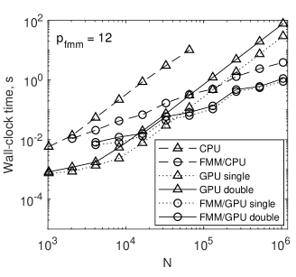
Figure 1: The wall-clock time required for a single MVP using different hardware and algorithmic accelerators (the time for generation of the data structure is not included). The data points are distributed randomly inside a unit cube. The time is measured on a PC equipped with a 12-core CPU (Intel Xeon 5660 2.8 GHz) and one GPU (NVIDIA Tesla K20).

Table 2: Acceleration of the MVP using different methods ($p_{fmm}=12$)

$N$	GPU		FMM	FMM+GPU
	single	double		single	double
4,096	40	31	3	8	7
16,384	111	44	13	66	54
65,536	86	33	31	157	125
262,144	87	33	125	395	339
1,048,576	87	33	667	2896	2309

Three methods are considered to accelerate the MVP: first, brute-force hardware (GPU) acceleration; second, algorithmic (FMM) acceleration (the time for generation of the data structure is neglected); and, third, algorithmic (FMM) + hardware (GPU) acceleration. Figure 1 demonstrates the dependence of the runtime for the MVP using these three approaches (also the times for single and double precision GPU computing are measured separately). It is seen that the complexity of the brute-force MVP implemented on the CPU or GPU is quadratic in $N$ while it is close to linear for the FMM implemented on CPU/GPU. In all cases the FMM was optimized (the optimal $l_{\max}$ was determined for each $N$; it is different for CPU and GPU, see Gumerov2008 ). Table 2 shows the accelerations achieved using the three methods mentioned. Here a CPU code implementing brute-force MVP is taken as a reference (for large $N$ the data for the reference case are extrapolated proportionally to $N^{2}$). It is seen that at large enough $N$ the GPU acceleration of the brute-force method stabilizes near some constants, and single precision computing 2.6 times faster than the double precision. The use of single precision in the GPU accelerated FMM brings smaller gains in speed. This table along with Fig. 1 also shows that for problem sizes $N\lesssim 30,000$ the use of a such complex algorithm as the FMM is not justified since the brute-force use of a GPU delivers the same or better accelerations of the reference code.

4 Numerical examples

The method described above is validated in many tests, some of which are presented below and can be used as benchmark cases when comparing different bubble dynamics codes. All numerical results presented in this paper (except the comparisons with the benchmark cases of Bui et al Bui2006 ) are obtained for air bubbles in water ($\rho=1000$ kg/m³, $\sigma=0.073$ Pa/m, $\kappa=1.4$) under atmospheric pressure ($p_{0}=10^{5}$ Pa) and zero gravity. To illustrate computations, the dimensionless coordinates $x^{\prime}=x/a_{0},\;y^{\prime}=y/a_{0},\;z^{\prime}=z/a_{0}$ are used, where $a_{0}$ is the initial bubble size/radius.

4.1 Single spherical bubble in an acoustic field

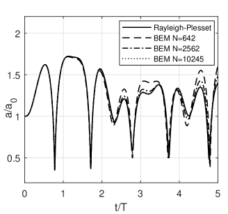
Figure 2: A comparison of the numerical solution at different surface discretizations with the solution of the Rayleigh-Plesset equation for a spherical bubble.

As a starting point, some tests for a single spherical bubble ($a_{0}=10$ $\mu m$) under the action of an acoustic field are conducted. The obtained results are compared with the solution of the Rayleigh-Plesset equation Plesset1977 at zero viscosity,

$$a\ddot{a}+\frac{3}{2}\dot{a}^{2}=\left[p_{g0}\left(\frac{a_{0}}{a}\right)^{3\kappa}-p_{\infty}\left(t\right)-\frac{2\sigma}{a}\right],$$ (59)

$$a(0)=a_{0},\quad\dot{a}(0)=0.$$

Figure 2 compares the dynamics of bubble radius using different number of boundary elements and the “exact” solution for the amplitude of the acoustic field $P_{a}=p_{0}$ and frequency $200$ kHz (period $T=5$ $\mu s$) (“exact” means error controlled numerical solution of ODE (59)). It is seen that the discretization has a little effect on the computed results at $t\leq 2T$, while for $t>2T$ substantially high $N$ is needed to reproduce the spherical bubble dynamics accurately. This phenomenon can be explained by the fact that the bubble shape approximated by the mesh is not exactly spherical. So, there exists some energy transfer between the volume and shape modes, which manifests itself at smaller times for smaller $N$.

It is noticeable that even this simple case cannot be computed without surface smoothing techniques. For the range of $N$ used in this example, the mesh was destabilized within 40-50 time steps without shape filtering (52 time steps at $N=642$, 40 time steps at $N=2562$, and 37 time steps at $N=10245$). The stability condition (33) requires smaller time steps at higher surface discretization. So the time $t_{\max}$ for computable solution without surface smoothing decreases at increasing $N$ ($t_{\max}/T=0.132,$ $0.0512,$ and $0.0229$ at $N=642,$ $2562,$ and $10245$, respectively). Utilization of the spherical filter at each time step with reasonable $p_{f}$ removes this instability and computations can proceed to a user-specified $t_{\max}.$

The term “reasonable $p_{f}$” requires some elaboration. In this and other cases reported below we found that at large enough $p_{f}$ ($p_{f}>10$) the surface destabilizes anyway (at later times compared to the computations without the surface smoothing, since the lower frequency shape instabilities develop anyway), while at small enough $p_{f}$ ($p_{f}<4$) details of shape deformation can be lost or reproduced incorrectly. We varied parameters $N_{d}$ and $p_{f}$ to check the correctness of the results. For example, computations of formation of jets in interacting bubbles are consistent for range $p_{f}=4,...,9$ and $N_{d}=642$ and $2562$. In the cases reproted below, one should assume $p_{f}=6$ and $N_{d}=642$ (if not stated otherwise).

4.2 Comparisons with some reported cases

There exist many studies of bubble dynamics in three dimensions demonstrating various shapes of the bubbles. Bui et al Bui2006 well documented 7 cases of different bubble configurations, which can be considered as benchmark cases. We computed several of these cases (only two of them are reported below) and found satisfactory qualitative and quantitative agreement with the data reported in Bui2006 . All cases Bui2006 are computed for simplified bubble dynamics model (underwater explosion resulting in a relatively large bubble), which follows from Eqs (8)-(10) at zero gravity, zero surface tension, and $F(t)=const.$ These equations coincide with the dimensionless equations of Bui et al at $F(t)\equiv 1$, $\epsilon=p_{0}/\rho$, $\lambda=\kappa$, where $\epsilon$ and $\lambda$ are the strength parameter and the gas polytropic exponent. All benchmark cases computed at $\epsilon=97.52$ and $\lambda=1.25$. Hence, if in our computations we set $\rho=10^{3}$ kg/m³, $p_{0}=0.9752\cdot 10^{5}$ Pa, then all dimensional variables in basic SI units (lengths in meters, time in seconds), will be the same as the respective dimensionless variables of the cited work.

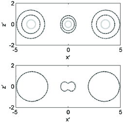
Figure 3: A comparison of the solution for three bubbles (the gray lines) with the Case 2 solution of Bui et al (2006) (the dashed lines) at the moments of time $t=0.05$ $s$ and $t=0.758$ $s$ (on the left plot) and at $t=2.65$ $s$ (on the right plot). The contour at $t=0.05$ $s$ of Bui et al corresponds to the shape at $t=0.3$ $s$ in the present computations (for comparisons, the shape at $t=0.05$ $s$ is also shown).

Figure 3 compares the results for the benchmark Case 2 (three equispaced bubbles in a row of initial distance between the centers 3.55 $m$, and radii for the central bubble $0.1499$ $m$ and $0.2379$ $m$ for the outer bubbles. It is seen that the shapes and positions of the bubbles agree well. The difference is explainable by different discretizations of the surface and the different numerical techniques (different ways of evaluation of boundary integrals, different surface smoothing procedures, etc.). Our estimates show that these factors can explain the relative differences in computed results of the order of several percents. It is also noticeable that the relative errors of the BEM alone (just because of the surface discretization by flat triangles) is a few percents, which also agrees with the estimates of Bui2006 . Note a misprint in Bui2006 for this case, as two moments of time $t=0.05$ $s$ and $0.758$ $s$ are reported for the growth phase. In fact, the reported contour at $0.05$ $s$ corresponds to a shape at $0.3$ $s$ in our computations (for comparisons we also show our result at $0.05$ $s$).

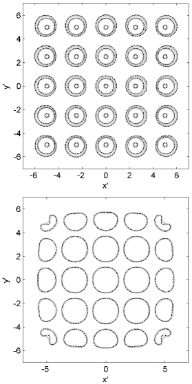
Figure 4: A comparison of the solution for 25 bubbles (the gray lines) with the Case 7 solution of Bui et al (2006) (the dashed lines) at the moments of time $t=0.01$ $s,$ $t=0.473$ $s$, and $t=0.923$ $s$ (on the left plot) and $t=2.854$ $s$ (the present work) and at $t=2.935$ $s$ (Bui et al) (on the right plot).

Comparisons of the present computations and the results reported in Bui2006 for the benchmark Case 7 ($25$ bubbles of initial equal size $0.1499$ $m$ at $t=0$ are arranged into a $5\times 5$ 2D grid with the minimal distance 2.5 $m$ between the bubble centers) are shown in Fig. 4. Again, one can see a satisfactory agreement between the results. Note that the pictures for the collapse stage obtained at time $t=2.854$ $s$, while Bui2006 reported the nondimensional time $t^{\prime}=2.939$. The difference between these moments is less than 3% and can be explained by the BEM errors and the differences in algorithms. The reason why the present computations were not continued beyond $t=2.854$ $s$ is that the corner bubbles changed their topology between $t=2.854$ $s$ and $t=2.939$ $s.$

4.3 Three bubbles in an acoustic field

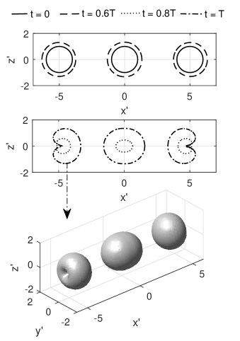
Figure 5: On the upper plots: the projections of the bubble shapes in an acoustic field at different moments of time $t$ for the test case a) ($T$ is the period of the acoustic field). The bottom plot showing shapes in 3D corresponds to $t=T$.

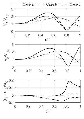
Figure 6: The dynamics of the volume of bubble #1 (on the top plot) and bubble #2 (in the middle plot), and the relative displacement of the mass center of bubble #1 (at the bottom plot) for test cases a) b) and c) (three bubbles in an acoustic field of period $T$).

To study bubble deformation and migration in an acoustic field we conducted small-scale tests for three bubbles located on the $x$-axis, and labeled as 1,2,3 (the central bubble is labeled as “#2” and the bubble with positive $x$-coordinate of the center is labeled as “#3”). In all cases, the distance $d$ between bubbles #1 and #2 is the same as the distance between bubbles #$2$ and #$3$. Three cases are reported below: a) the initial radii of all bubbles are the same, $a_{10}=a_{20}=a_{30}=a_{0}=10$ $\mu m$, the initial distance between the bubble centers is $d=5a_{0}$; b) $a_{10}=a_{30}=a_{0}=10$ $\mu m$, $a_{20}=2a_{0}$, $d=6a_{0}$; c) $a_{20}=a_{0}=10$ $\mu m$, $a_{10}=a_{30}=2a_{0}$, $d=6a_{0}$. In all cases, the acoustic field of frequency 200 $kHz$ ($T=5$ $\mu s$) has amplitude $P_{a}=0.7p_{0}$.

In case a) the qualitative picture is the following. At $0<t/T<0.55$ all bubbles grow in volume and bubbles #1 and #3 slightly repel from the central bubble while remaining spherical. At time $0.55<t/T<0.8$ bubbles collapse and bubbles #1 and #3 move towards the central bubble, which takes some elongated, ellipsoid-like shape. The bubble volume achieves its minimum at $t/T<0.8$ after which all bubbles start to grow again, while still attracting. In fact, this attraction of the bubble mass centers is due to the formation of jets in bubbles #1 and #3 directed towards the central bubble. Bubble #$2$ is also non-spherical and has some prolate spheroid shape. Contours of bubble shape projection on the $y=0$ plane and the shapes of the bubbles at $t/T=1$ are shown in Fig. 5.

The bubble dynamics in case b) is different from that observed in case a). Here the more massive bubble in the center remains almost spherical all the time. The deformation of bubbles #1 and #3 is not so strong as in case a). Moreover, the jets are not formed in these bubbles, but at $t/T=1$ they become pear-shaped tapering in the direction away from bubble #2. Case c) is different from both cases a) and b). Here bubbles #1 and #3 are almost spherical at $0\leqslant t/T\leqslant 1$, while qualitatively (not quantitatively) the dynamics of bubble #2 is similar to the dynamics of bubble #2 in case a). At $t/T=1$ it looks like a prolate spheroid. Figure 6 shows the relative bubble volume as a function of time for all three cases. It also demonstrates the dynamics of the mass center of bubble #1.

4.4 Bubble clusters in an acoustic field

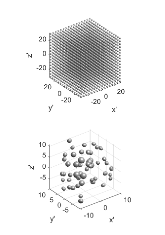
Figure 7: Views of the largest $16\times 16\times 16$ regular cluster (on the top plot) used in the present study at $t=0$. A view of a random ($M=51$) monodisperse cluster in an acoustic field of period $T$ at $t=T$ (on the bottom plot).

Using the present algorithm, we studied dynamics of monodisperse bubble clusters of different sizes and configuration. Figure 7 shows the largest regular cluster used in the present tests ($M=4096$, $N=2,629,632$, $a_{0}=10$ $\mu m$), and a random monodisperse cluster ($M=51,$ $N=32,742,$ $a_{0}=10$ $\mu m$). Mention that for large clusters in acoustic fields condition $D_{cl}/\lambda\ll 1$ ($D_{cl}$ is the cluster size and $\lambda$ is the acoustic wavelength) should hold to justify the assumption that the liquid is incompressible. For example, the wavelength of 200 kHz sound in water is $\lambda=$7.5 mm and for the largest case shown in Fig. 7 we have $D_{cl}/\lambda=0.08$ ($M=4096$).

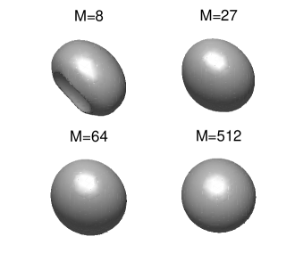
Figure 8: The shapes of the corner bubbles in $n_{b}\times n_{b}\times n_{b}$ clusters ($n_{b}=2,3,4,8;$ $M=n_{b}^{3}$) at $t=0.9T$ ($M=8$) and $t=T$ ($M=27,64,512$).

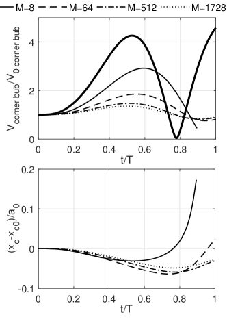
Figure 9: On the top plot: the dynamics of the volume of the corner bubble in $n_{b}\times n_{b}\times n_{b}$ clusters ($n_{b}=1,2,4,8,12;$ $M=n_{b}^{3}$) in an acoustic field of period $T$. At the bottom plot: the $x$-coordinate of the relative displacement of the mass center of the corner bubble in the respective clusters.

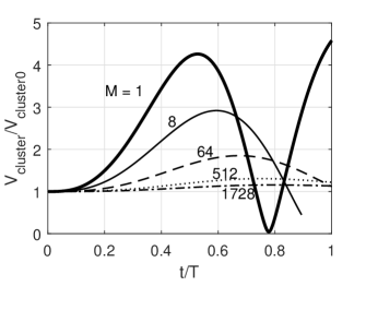
Figure 10: The dynamics of the volume of $n_{b}\times n_{b}\times n_{b}$ bubble clusters ($n_{b}=1,2,4,8,12;$ $M=n_{b}^{3}$) in an acoustic field of period $T$.

Figures 8 - 10 provide some data, which can be used for validation of this and other bubble dynamic codes. In these case bubble cluster arranged in a $n_{b}\times n_{b}\times n_{b}$ cubic grid ($n_{b}=1,...,16$) consisting of spherical bubbles of initial size $a_{0}=10$ $\mu m$ is placed in an acoustic field of frequency 200 $kHz$ ($T=5$ $\mu s$) and amplitude $P_{a}=p_{0}$. The initial distance between the closest bubble centers ($n_{b}>1$) is $d=4a_{0}$. Figure 8 shows the shapes of the corner bubble (the bubble with the minimum $x,y,z$ coordinates of the centers) at $t/T=1$ ($t/T=0.9$ in case $n_{b}=2$, which is approximately the moment of time when the bubble topology changed from spherical to toroidal). It is seen that as the cluster size increases the shape of this bubble becomes closer to spherical. In fact, the corner bubbles are the most deformed bubbles in the cluster, so the other bubbles are more spherical. Figure 9 illustrates the dynamics of the volume of the corner bubble and the change of the relative $x$-coordinate of its center. Hence, the larger cluster, the weaker the response to variations of the external pressure field. Figure 10 showing the dynamics of the volume of the entire cluster also supports this conclusion.

4.5 Performance

Finally, we report some figures about the overall performance of the developed code. The wall-clock time is measured for the work station described above. The most critical issue here is the scaling of the code with $N$. For this study one can use the cases with bubbles arranged in a $n_{b}\times n_{b}\times n_{b}$ cubic grid at different $n_{b}$.

Table 3 shows profiling of the FMM/GPU code for $n_{b}=12$ and $n_{b}=16$ for two different accuracy settings. The faster option corresponds to single precision GPU computing, $p_{fmm}=8$, and the tolerance for the GMRES convergence $\epsilon_{gmres}=10^{-4}$. The other option is realized using double precision GPU computing, $p_{fmm}=12,$ and $\epsilon_{gmres}=10^{-5}$. The relative errors of these solutions are measured by comparisons with a more accurate (reference) solution (the reference solution is obtained using double precision, $p_{fmm}=16,$ and $\epsilon_{gmres}=10^{-6}$ ; in all cases the spherical filter of bandwidth $p_{f}=9$ was used):

$$\epsilon\left(t\right)=\frac{\left\|\mathbf{x}\left(t\right)\mathbf{-x}_{ref}\left(t\right)\right\|_{2}}{\max_{0<\tau<t}\left\|\mathbf{x}_{ref}\left(\tau\right)\mathbf{-x}_{ref}\left(0\right)\right\|_{2}}.$$ (60)

Here $\mathbf{x}\left(t\right)$ and $\mathbf{x}_{ref}\left(t\right)$ are the coordinates of the surface points for the testing and reference solutions, and $\left\|{}\right\|_{2}$ is the $L_{2}$-norm. The reason for normalization (60) opposed to $\left\|\mathbf{x}_{ref}\right\|_{2}$ is that $\left\|\mathbf{x}_{ref}\right\|_{2}$ for large clusters is large compared to perturbations of the bubble surface. As a result we have a low relative $L_{2}$-norm error, $\epsilon_{2}=\left\|\mathbf{x-x}_{ref}\right\|_{2}/\left\|\mathbf{x}_{ref}\right\|_{2}$, even for $\epsilon\sim 1$ (in our cases $\epsilon_{2}\left(t\right)/\epsilon\left(t\right)\lesssim 10^{-2}$). In metrics (60), we obtained for the first option $\epsilon=5.3\cdot 10^{-3}$, while for the second option $\epsilon=2.5\cdot 10^{-4}$ (both at the 200th step).

Table 3: Profiling of the FMM/GPU code (wall-clock time in seconds)

	$N=1,109,376$		$N=2,629,632$
	single	double	single	double
Filter	0.12	0.18	0.25	0.37
Surface	0.06	0.08	0.14	0.20
FMM DS	0.8	0.8	2.8	2.8
# MVPs	12	15	12	16
1 MVP	0.64	1.3	1.9	4.0
BEM MVP	9.4	21.6	26.8	70.0
Time Step	10.0	22.3	28.1	71.6

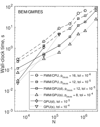
Figure 11: The wall-clock time required for the BEM iterative solver as a function of the number of the mesh vertices $N$ of $n_{b}\times n_{b}\times n_{b}$ bubble clusters. The tests are performed using single and double precision computing on GPU (marked as “s” and “d”), different tolerances for the GMRES relative residual norm $\epsilon_{gmres}$ (denoted as “tol”), and the FMM truncation numbers $p_{fmm}$ (if the FMM is employed). The wall-clock times are measured on the same PC as in Fig. 2.

The profile is measured for one typical time step (the 200th step from the start; the “warm-up” initial steps are more expensive). The table shows that the time for filtering applied twice for one right-hand side call is really small compared to the time for the BEM solution (the filtering is performed on GPU). The same applies to computations of the necessary surface functions (briefly called “Surface”). These functions include computations of normals, areas, curvature, volume, and the tangential velocity and implemented on GPU. The BEM solution requires the FMM data structure (“FMM DS”), which computational cost normally does not exceed 10% of the cost of the solution. The most time is spent performing MVP. The Matlab standard GMRES solver requires $n_{iter}+2$ MVP’s for $n_{iter}$ iterations. Four MVP’s are needed to compute the singular BEM integrals, and one MVP is needed to compute the right-hand side vector in Eq. (19). So, the total number of MVP’s per time step of the AB6 solver is $n_{iter}+7$, which for 2-10 GMRES iterations results in 9-17 MVP calls.

Figure 11 illustrates the wall-clock time required for the BEM iterative solver. The MVP is performed using hardware and algorithmic accelerators. Here several options with different $p_{fmm}$ and tolerance $\epsilon_{gmres}$ are compared. It is seen that the brute-force GPU acceleration can be used efficiently for $N\lesssim 2\cdot 10^{4}$. For larger $N$ combination FMM/GPU provides better performance.

5 Conclusions

We developed and tested an efficient numerical method, which enables simulations of bubble systems with dynamic deformable interfaces discretized by millions of boundary elements on personal supercomputers. It is shown that for small and midsize ($N\lesssim 20,000$) problems GPU acceleration alone is more efficient than the FMM/GPU acceleration, while for the solution of large-scale problems the use of a scalable algorithm, such as the FMM is critical. The use of GPU in the FMM brings considerable accelerations (several times) compared to the FMM on CPU alone for the hardware used in the present study. However, utilization of many-core CPUs substantially reduces the effect of GPUs in the FMM, and GPU accelerations are much smaller than that reported in Gumerov2008 . The scaling of the algorithm obtained in this study enables estimations of the computational time and resources for distributed computing clusters.

The algorithm is implemented and validated against simplified solutions and solutions published in the literature. While some differences in solutions are observed, they are explainable and do not exceed several percents typical for solutions obtained using boundary elements. Also, validation of the developed code was performed using different surface discretizations and different parameter settings controlling the accuracy and stability of the algorithm. One of the new elements implemented and tested is a shape filter, which showed its effectiveness for mesh stabilization and efficiency regarding performance. Profiling of the algorithm indicates that the most time is spent on MVPs, while the overheads related to filtering, generation of the data structure, etc. are reasonably small. It is interesting that substantial reduction of the accuracy of computations (single precision GPU) brings 2x accelerations, while the overall accuracy and stability are still acceptable (the errors are much smaller than the discretization and other BEM errors). The code can be used in many studies related to bubble dynamics, and such applications are envisioned in future.

References

- (1) Brennen CE (2014) Cavitation and Bubble Dynamics. Cambridge University Press, New York
- (2) Xi X, Cegla F, Mettin R, Holsteyns F, Lippert A (2012) Collective bubble dynamics near a surface in a weak acoustic standing wave field. J Acoust Soc Am 132:37-47
- (3) Ovenden NC, O’Brien JP, Stride E (2017) Ultrasound propagation through dilute polydisperse microbubble suspensions. J Acoust Soc Am 142:1236-1248
- (4) Nigmatulin RI (1991) Dynamics of Multiphase Media. Hemisphere, Washington DC
- (5) Plesset MS, Prosperetti A (1977) Bubble dynamics and cavitation. J Fluid Mech 9:145-185
- (6) Akhatov I, Gumerov N, Ohl C-D, Parlitz U, Lauterborn W (1997) The role of surface tension in stable single–bubble sonoluminescence. Phys Rev Lett 78:227-230
- (7) Khabeev NS (2009) The structure of roots of characteristic equation for free oscillations of a gas bubble in liquid. Doklady Physics 54:549-552
- (8) Lauterborn W, Kurz T (2010) Physics of bubble oscillations. Rep Prog Phys 73:106501
- (9) Parlitz U, Mettin R, Luther S, Akhatov I, Voss M, Lauterborn W (1999) Spatiotemporal dynamics of acoustic cavitation bubble clouds. Phil Trans R Soc Lond A 357:313-334
- (10) Gumerov NA, Akhatov IS (2012) Numerical simulation of 3D self-organization of bubbles in acoustic fields Proceedings of the 8th International Symposium on Cavitation, Singapore 189
- (11) Voinov VV, Voinov OV (1975) Numerical method of calculating nonstationary motions of an ideal incompressible fluid with free surfaces. Sov Phys Doklady 20:179-182
- (12) Blake JR, Gibson DC (1987) Cavitation bubbles near boundaries. Ann Rev Fluid Mech 19:99-123
- (13) Best JP, Kucera A (1992) A numerical investigation of nonspherical rebounding bubbles. J Fluid Mech 245:137-154
- (14) Boulton-Stone JM (1993) A comparison of boundary integral methods for studying the motion of a two-dimensional bubble in an infinite fluid. Comput Methods Appl Mech Eng 102:213-234
- (15) Boulton-Stone JM (1993) A two-dimensional bubble near a free surface. J Eng Math 27:73-87
- (16) Oguz HN, Prosperetti A (1990) Bubble oscillations in the vicinity of a nearly plane free surface. J Acoust Soc Am 87:2085-2092
- (17) Oguz HN, Prosperetti A (1993) Dynamics of bubble growth and detachment from a needle. J Fluid Mech 257:111-145
- (18) Chahine GL, Duraiswami R (1992) Dynamical interactions in a multibubble cloud. ASME J Fluids Eng 114:680-686
- (19) Chahine GL (1994) Strong interactions bubble/bubble and bubble/flow. Bubble Dynamics and Interface Phenomena: Proceedings of an IUTAM Symposium held in Birmingham, U.K.:195-206
- (20) Zhang S, Duncan JH, Chahine GL (1993) The final stage of the collapse of cavitation bubble near a rigid wall. J Fluid Mech 257:147-181
- (21) Zhang YL, Yeo KS, Khoo BC, Wang C (2001) 3D jet impact and toroidal bubbles. J Comput Phys 166:336-360.
- (22) Gumerov NA, Chahine GL (2000) An inverse method for the acoustic detection, localization and determination of the shape evolution of a bubble. Inverse Problems 16:1741-1760
- (23) Itkulova YuA, Abramova OA, Gumerov NA, Akhatov IS (2014) Boundary element simulations of free and forced bubble oscillations in potential flow. Proceedings of the ASME International Mechanical Engineering Congress and Exposition, Montreal, Quebec, Canada, Paper No. 36972
- (24) Lee M, Klaseboer E, Khoo BC (2007) On the boundary integral method for the rebounding bubble. J Fluid Mech 570:407-429
- (25) Pozrikidis C (2003) Computation of the pressure inside bubbles and pores in Stokes flow. J Fluid Mech 474:319-337
- (26) Itkulova YuA, Abramova OA, Gumerov NA (2013) Boundary element simulations of compressible bubble dynamics in Stokes flow. Proceedings of the ASME International Mechanical Engineering Congress and Exposition, San Diego, California, Paper No. 63200
- (27) Bui TT, Ong ET, Khoo BC, Klaseboer E, Hung KC (2006) A fast algorithm for modeling multiple bubbles dynamics. J Comp Physics 216:430-453
- (28) Prosperetti A, Trygvasson G (2007) Computational Methods for Multiphase Flow. Cambridge University Press, New York
- (29) Magnaudet J, Eames I (2000) The motion of high-Reynolds-number bubbles in inhomogeneous flows. Ann Rev Fluid Mech 32:659-708
- (30) Greengard L, Rokhlin V (1987) A fast algorithm for particle simulations. J Comp Phys 73:325-348
- (31) Cheng H, Greengard L, Rokhlin V (1999) A fast adaptive multipole algorithm in three dimensions. J Comput Phys 155:468-498
- (32) Gumerov NA, Duraiswami R (2008) Fast multipole methods on graphics processors. J Comput Phys 227:8290-8313
- (33) Gumerov NA, Duraiswami R (2005) Comparison of the efficiency of translation operators used in the fast multipole method for 3D Laplace equation. Technical Report CS-TR-4701, College Park, University of Maryland
- (34) Nishimura N (2002) Fast multipole accelerated boundary integral equation methods. Appl Mech Rev 55(4):299-324
- (35) Gumerov NA, Duraiswami R (2006) FMM accelerated BEM for 3D Laplace and Helmholtz equations. Proceedings of the International Conference on Boundary Element Techniques VII, BETEQ-7, Paris, France, EC Ltd., UK:79-84
- (36) Liu Y (2009) Fast Multipole Boundary Element Method: Theory and Applications in Engineering. Cambridge University Press, New York
- (37) Greengard L, Gropp WD (1990) A parallel version of the fast multipole method. Computers Math Applic 20:63-71
- (38) Hu Q, Gumerov NA, Duraiswami R (2011) Scalable fast multipole methods on distributed heterogeneous architectures. Proceedings of International Conference for High Performance Computing, Networking, Storage, and Analysis, SC’11, ACM, New York, NY:36:1-36:12
- (39) Hu Q, Gumerov NA, Duraiswami R (2012) Scalable distributed fast multipole methods. Proceedings of 2012 IEEE 14th International Conference on High Performance Computing and Communications, UK, Liverpool:270-279
- (40) Itkulova YuA, Solnyshkina OA, Gumerov NA (2012) Toward large scale simulations of emulsion flows in microchannels using fast multipole and graphics processor accelerated boundary element method. Proceedings of the ASME International Mechanical Engineering Congress and Exposition, Houston, Texas Paper No. 86238
- (41) Abramova OA, Itkulova YuA, Gumerov NA (2013) FMM/GPU accelerated BEM simulations of emulsion flow in microchannels. Proceedings of the ASME International Mechanical Engineering Congress and Exposition, San Diego, California Paper No. 63193
- (42) Abramova OA, Itkulova YuA, Gumerov NA, Akhatov ISh (2014) An efficient method for simulation of the dynamics of a large number of deformable droplets in the Stokes regime. Doklady Physics 59:236-240
- (43) Hu Q, Gumerov NA, Duraiswami R (2013) GPU accelerated fast multipole methods for vortex particle simulation. Computers & Fluids 88:857-865
- (44) Maryin DF, Malyshev VL, Moiseeva EF, Gumerov NA, Akhatov IS (2013) Acceleration of molecular dynamics modeling using fast multipole method and graphics processors. Numerical Methods and Programming, 14:483-495 (in Russian).
- (45) Adelman R, Gumerov NA, Duraiswami R (2017) FMM/GPU-accelerated boundary element method for computational magnetics and electrostatics. IEEE Transactions on Magnetics 53:7002311
- (46) Lashuk I, Chandramowlishwaran A, Langston H, Nguyen T, Sampath R, Shringarpure A, Vuduc R, Ying L, Zorin D, Biros G (2009) A massively parallel adaptive fast-multipole method on heterogeneous architectures, in: Proceedings of the Conference on High Performance Computing Networking, Storage and Analysis, SC’09, Portland, Oregon:1-12
- (47) Rahimian A, Lashuk I, Veerapaneni S, Chandramowlishwaran A, Malhotra D, Moon L, Sampath R, Shringarpure A, Vetter J, Vuduc R, Zorin D, Biros G (2010) Petascale direct numerical simulation of blood flow on 200 k cores and heterogeneous architectures. Proceedings of the 2010 ACM/IEEE International Conference for High Performance Computing, Networking, Storage and Analysis, SC’10, IEEE Computer Society:1-11
- (48) Yokota R, Barba LA, Narumi T, Yasuoka K (2013) Petascale turbulence simulation using a highly parallel fast multipole method on GPUs. Comput Phys Comm 184:445-455
- (49) Chen LH, Zhou J (1992) Boundary Element Methods. Academic Press, New York
- (50) Adelman R, Gumerov NA, Duraiswami R (2016) Computation of the Galerkin double surface integrals in the 3-D boundary element method. IEEE Trans Antennas and Propag 64:1-13
- (51) Gumerov NA, Duraiswami R (2009) A broadband fast multipole accelerated boundary element method for the 3D Helmholtz equation. J Acoust Soc Am 125:191-205
- (52) Klaseboer E, Rosales-Fernandez C, Khoo BC (2009) A note on true desingularization of boundary element methods for three-dimensional potential problems. Engng Anal Bound Elem 33:796-801
- (53) Saad Y (1993) A flexible inner-outer preconditioned GMRES algorithm. SIAM J Sci Comput 14:461-469
- (54) Saad Y, Schultz MH (1986) GMRES: A generalized minimal residual algorithm for solving nonsymmetric linear systems. SIAM J Sci Stat Comput 7:856-869
- (55) Zinchenko AZ, Rother MA, Davis RH (1997) A novel boundary-integral algorithm for viscous interaction of deformable drops. Phys Fluids. 9:1493-1511
- (56) Gumerov NA, Duraiswami R (2004) Fast Multipole Methods for the Helmholtz Equation in Three Dimensions. Elsevier, Oxford