Dynamics of particle uptake at cell membranes

Abstract

Receptor-mediated endocytosis requires that the energy of adhesion overcomes the deformation energy of the plasma membrane. The resulting driving force is balanced by dissipative forces, leading to deterministic dynamical equations. While the shape of the free membrane does not play an important role for tensed and loose membranes, in the intermediate regime it leads to an important energy barrier. Here we show that this barrier is similar to but different from an effective line tension and suggest a simple analytical approximation for it. We then explore the rich dynamics of uptake for particles of different shapes and present the corresponding dynamical state diagrams. We also extend our model to include stochastic fluctuations, which facilitate uptake and lead to corresponding changes in the phase diagrams.

I Introduction

The plasma membrane presents a physical barrier that separates the interior of the cell from its environment. Therefore, the ability of cells to exchange information and material across their plasma membrane is of central importance for their function Auth et al. (2018); Zhang et al. (2015). On the one hand, these uptake processes are vital for nutrient influx and signal transduction Alberts et al. (2017). On the other hand, pathogens like viruses hijack cellular uptake processes to enter host cells during infections Kumberger et al. (2016). In addition, uptake of artificial particles at cell membranes can be desired, as e.g. in the context of drug delivery Panyam and Labhasetwar (2003), or undesired, as e.g. in the context of microplastics von Moos et al. (2012).

In receptor-mediated endocytosis particles with sizes between $10-300\,\mathrm{nm}$ are taken up because the energy gain upon particle binding to cell surface receptors overcomes the deformation energy of the membrane Gao et al. (2005). Membrane shape is of central importance for this process. It is fixed by particle shape at the adhered part, but follows from minimization of the membrane energy for the free part, compare Fig. 1. Very importantly, cargo particles can come with a huge diversity in shape, including the case of viruses. The most frequent virus shape is the spherical or icosahedral shape, followed by filamentous and then by more complex shapes. To name a few examples, reovirus, causing respiratory or gastrointestinal illnesses, has icosahedral shape Barton et al. (2001), Marburg or Ebola viruses have filamentous shape Feldmann et al. (2003), and rabies virus has bullet-like shape Matsumoto (1963). Apart from shape, stochastic fluctuations in receptor binding might also play a role, as the cargo particles are small and typically covered by only few tens of ligands.

The uptake of small particles has been previously studied both analytically and by computer simulations. Deterministic approaches usually focus on calculating minimal energy shapes for the plasma membrane and the attached particle to deduce dynamical state diagrams Lipowsky and Döbereiner (1998); Deserno (2004); Agudo-Canalejo and Lipowsky (2015), investigate uptake dynamics and the role of receptor diffusion within the plasma membrane Gao et al. (2005); Decuzzi and Ferrari (2007), study the consequences of particle elasticity during uptake Yi et al. (2011); Zeng et al. (2017) or interactions of the particle and the cytoskeleton Sun and Wirtz (2006). Stochastic approaches usually focus on the effect of ligand-receptor binding Yi and Gao (2017). Computer simulations complement these studies by considering especially the role of non-spherical particle geometries Vácha et al. (2011); Huang et al. (2013); Dasgupta et al. (2014); Bahrami et al. (2014); Deng et al. (2019) or the role of scission, when the wrapped particle is separated from the membrane McDargh et al. (2016).

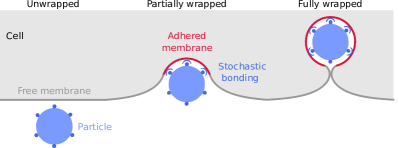
Figure 1: During receptor-mediated endocytosis, the particle goes from unwrapped through partially wrapped to fully wrapped. While membrane shape is fixed by particle shape in the region of the adhered membrane (red part of the contour), the shape of the free membrane follows from an energy minimization (grey part of the contour).

Despite this plethora of different approaches, analytical approaches are rare that allow us to study the interplay of particle shape, free membrane shape and stochasticity in one transparent framework. Recently we showed that in a deterministic model, spherical particles are taken up slower compared to cylindrical particles, whereas the situation can reverse in a stochastic description, because spherical particles profit more from the presence of noise Frey et al. (2019). However, in this earlier work we have neglected the exact role of the free part of the membrane and did not investigate the possibility that the dynamics stops with a partially wrapped particle (Fig. 1). Earlier it has been suggested that the free membrane might act as an effective line tension Lipowsky and Döbereiner (1998) and exact formulae for the elastic energy barrier provided by the free membrane have been derived for the limits of tense and loose membranes Foret (2014). Here we present a comprehensive study of these important effects and show that in the general case, a simple term that is similar to but different from a line tension term describes this energy barrier well. With this simplification, we are able to perform a comprehensive analysis of the uptake dynamics at membranes, including the effect of particle shape and stochastic fluctuations. By combining models for membrane mechanics, overdamped membrane dynamics and stochastic dynamics of receptor-ligand binding, we find a very rich scenario of possible uptake dynamics.

Our work is organized as follows. In section II we first calculate the shape and energy of the free membrane by numerically solving the shape equations that give the minimal energy shapes of the free membrane. By comparing this energy to the energy of the adhered membrane we can identify the parameter regime in which the free membrane cannot be neglected, as it contributes up to $20\%$ of the total energy. We also show that this energy contribution is similar to but different from the effect of a line tension; in particular, it leads to faster initial uptake and the associated energy barrier is located at higher coverage. These effects can be described well by a simple analytical ansatz introduced here. In section III we derive and analyze the deterministic dynamical equations for cylindrical, spherical and spherocylindrical particles. Here the free membrane is not yet taken into account explicitly, but its potential effect can already be appreciated on the level of a line tension. We find that spherical particles are taken up slower than cylindrical particles. In addition, we find that short cylinders are taken up faster in normal orientation, whereas long cylinders are taken up faster in parallel orientation. For spherocylindrical particles we find that they are taken up fastest in parallel orientation. In section IV we include the analytically exact energy of the free membrane for parallel cylindrical particles into our dynamical model and calculate dynamical state diagrams. In addition, we also include free membrane effects by the phenomenological approach. As the phenomenological approach gives similar results, we then apply our approach also to spherical particles. In section V we calculate dynamical state diagrams for spherical particles using the phenomenological ansatz. We identify three regimes: full uptake, partial uptake and no uptake determined by membrane elasticity, adhesion energy and the free membrane. In section VI we then extend our model to a stochastic description, which in contrast to earlier work Frey et al. (2019) now includes the effect of the free membrane. We find that fluctuations decrease uptake times and expand uptake to parameters regions where uptake is not possible in the deterministic model. In addition, we find that spherical particles can be taken up faster with fluctuations compared to parallel cylindrical particles.

II Membrane energies

To arrive at a dynamical model for particle uptake at cell membranes, we follow the standard approach and first compare the energy gain due to adhesion and the energy cost due to bending and tension Lipowsky and Döbereiner (1998); Deserno (2004); Agudo-Canalejo and Lipowsky (2015); Auth et al. (2018). Later we will introduce dynamics by also considering dissipative forces. We are interested in ligand-receptor interactions and for simplicity assume that they are distributed homogeneously over the particle surface. The total energy of the membrane is then described by the following generalization of the Helfrich bending Hamiltonian Helfrich (1973)

$$E=-\int_{A_{\mathrm{ad}}}W\mathrm{d}A+\int_{A_{\mathrm{mem}}}2\kappa H^{2}\mathrm{d}A+\sigma\Delta A+\zeta\mathcal{E}\,.$$ (1)

The first term is the gain in adhesion energy, where the adhesion energy per area $W$ is defined to be positive. The second term is the bending energy with $\kappa$ being the bending rigidity and $H$ the mean curvature of the membrane. The third term is the tension energy, with $\sigma$ being the membrane tension and $\Delta A$ the excess area compared to the flat membrane. It is important to note that only the part $A_{\mathrm{ad}}$ of the membrane that adheres to the particle contributes to the adhesion energy, while both the adhered and the free parts of the membrane, $A_{\mathrm{mem}}=A_{\mathrm{ad}}+A_{\mathrm{free}}$, contribute to bending and tension (compare Fig. 1). The last term in Eq. (1) results from a possible line tension $\zeta$, with $\mathcal{E}$ being the length of the edge between the membrane adhering to the particle and the free cell membrane. We note that in general Eq. (1) also includes a term that depends on Gaussian curvature. However, since we do not consider topological changes, it can be neglected in our context Deserno (2004).

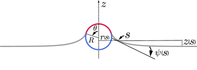
Figure 2: Parametrization of membrane shape for a spherical particle. The adhered part of the membrane is shown in red, the free part of the membrane is shown in grey and the particle is shown in blue. $R$ is the particle radius, $\theta$ is the uptake angle and $s$ the contour length of the free membrane. Tangent angle $\psi$, radial distance $r$ and height $z$ are functions of $s$.

The two membrane parameters $\kappa$ and $\sigma$ define a typical length scale $\lambda=\sqrt{\kappa/\sigma}$. Using this scale, the membrane can be classified as tense ($\lambda/R\ll 1$) or loose ($\lambda/R\gg 1$). Considering typical parameter values occurring in the context of particle uptake at cell membranes, $\kappa=25\,{k_{\mathrm{B}}T}$ and $\sigma=10^{-5}-10^{-3}{\rm N/m}$ Foret (2014); Kumar and Sain (2016), one has $\lambda=10-100\,{\rm nm}$. As typical sizes for virus or nanoparticles range from $R=10-100\,{\rm nm}$, it holds that $\lambda/R\sim 0.1-10$ and the biologically most relevant regime is hence intermediate between tense and loose.

The line tension term in Eq. (1) could result e.g. from the localization of certain lipids or proteins to the curved membrane at the border between the adhered and free membrane Lipowsky (1992). More importantly in our context, however, such a term could potentially also be used to describe the effective behaviour of the free membrane, even in the absence of a microscopic line tension Lipowsky and Döbereiner (1998). In this case, one could restrict the integration of the bending energy over the adhered part of the membrane. For dimensional reasons, one then would expect the effective line tension to scale as $\zeta=\sqrt{\kappa\sigma}$ and the typical range would be $\zeta=1-10\,{\rm pN}$ Deserno (2004); Foret (2014).

In order to discuss the role of the free membrane shape in more detail, let us consider the uptake of a spherical particle. Fig. 2 shows the used parametrization Foret (2014, 2018), where $\theta$ is the uptake angle, measured with respect to the symmetry axis (along the $z$-direction). The membrane contour is parameterized by its arc length $s$ relative to the point where the adhering membrane is connected to the free part. Furthermore, $\psi(s)$ is the angle between the radial axis normal to the $z$-axis and the contour tangent, $r(s)$ is the radial distance to the $z$-axis, and $z(s)$ the height. Note that $r$ and $z$ can be obtained by integration over $\psi$.

For the spherical particle, the area adhering to the membrane as a function of particle radius $R$ and uptake angle $\theta$ is given by $A_{\mathrm{ad}}=2\pi R^{2}(1-\cos\theta)$ and thus the adhesion energy would be $E^{\mathrm{W}}=-2\pi WR^{2}(1-\cos\theta)$. Similarly, also the contributions from bending and tension of the adhered part can be given explicitly. In the following, we non-dimensionalize energies by the bending rigidity. Then the total mechanical energy of the adhered part, $E_{\mathrm{ad}}^{\mathrm{tot}}=E_{\mathrm{ad}}^{\mathrm{\kappa}}+E_{\mathrm{ad}}^{\mathrm{\sigma}}$, reads

$$\frac{E_{\mathrm{ad}}^{\mathrm{tot}}}{\kappa}=4\pi(1-\cos\theta)+\pi\frac{R^{2}}{\lambda^{2}}(1-\cos\theta)^{2}\,.$$ (2)

For the energy of the free parts, $E_{\mathrm{free}}^{\mathrm{tot}}=E_{\mathrm{free}}^{\mathrm{\kappa}}+E_{\mathrm{free}}^{\mathrm{\sigma}}$, one has Foret (2014, 2018)

$$\frac{E_{\mathrm{free}}^{\mathrm{tot}}}{\kappa}=\pi\int_{0}^{\infty}\left(\dot{\psi}+\frac{\sin\psi}{r}\right)^{2}r\,\mathrm{d}s+\frac{2\pi}{\lambda^{2}}\int_{0}^{\infty}(1-\cos\theta)\,r\,\mathrm{d}s\,.$$ (3)

This energy has to be minimized with respect to the free membrane shape at given uptake angle $\theta$. Together with the geometrical relations between $\psi$, $r$ and $z$, one gets the following shape equations Seifert et al. (1991); Jülicher and Seifert (1994); Lipowsky and Döbereiner (1998); Deserno (2004); Foret (2014):

$$\ddot{\psi}r^{2}\cos\psi+\dot{\psi}r\cos^{2}\psi+\frac{1}{2}\dot{\psi}^{2}r^{2}\sin\psi$$

$$-\frac{1}{2}(\cos^{2}\psi+1)\sin\psi-\frac{r^{2}}{\lambda^{2}}\sin\psi =0,$$

$$\dot{r}-\cos\psi =0,$$

$$\dot{z}+\sin\psi =0\,.$$ (4)

This set of ordinary differential equations has to be solved with the boundary conditions

$$r(0)=R\sin\theta,\;\;\psi(0) =\theta,\;\;\psi(\infty)=0,\;\;\dot{\psi}(\infty)=0$$ (5)

and an additional one, $z(\infty)=0$, where other choices are also possible.

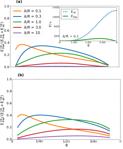
Figure 3: (a) The bending and tension energy of the free membrane relative to the total bending and tension energy, i.e. of the adhered and free parts of the membrane for different values of $\lambda/R$. To calculate the energy of the free parts we use Eq. (52) in the case of $\lambda/R<1$ and Eq. (53) in the case of $\lambda/R>1$ and the numerical solution for $\lambda=R$. The inset shows the bending and tension energy of the adhered and free parts of the membrane for $\lambda/R=0.1$. (b) The same as in (a) but for the phenomenological description of the free membrane given in Eq. (9).

We solved the boundary-value problem for the given system of ODEs from Eqs. (4) using a 4-th order collocation algorithm with matched asymptotics Sol . Details can be found in appendix A. We then evaluated the energy contributions from the free membrane. In addition, we compared to asymptotic expressions that have been given previously Foret (2014) for the limit of a tense ($\lambda/R\ll 1$) and loose membrane ($\lambda/R\gg 1$), which are also given in appendix A. In general, in both limits we get excellent agreement between these analytical and our numerical results.

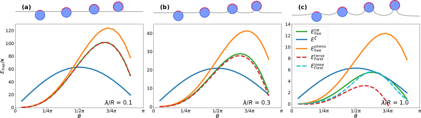
Figure 4: Energies of the free membrane for (a) $\lambda/R=0.1$, (b) $\lambda/R=0.3$ and (c) $\lambda/R=1.0$. The numerically calculated total energy of the free membrane is shown in green, the line tension approximation $E^{\zeta}$ is shown in blue, the phenomenological approximation $E_{\mathrm{free}}^{\mathrm{pheno}}$ from Eq. (9) is shown in orange and the analytical limits for tense (from Eq. 52 Foret (2014)) and loose (from Eq. 53 Foret (2014)) membranes are shown as dashed curves in red and cyan, respectively. (Top) Numerically calculated shapes of the membrane.

Fig. 3(a) shows the mechanical energy of the free membrane relative to the total mechanical energy for different values of $\lambda/R$. Here the energies of the free parts were calculated using Eq. (52) for the tense regime ($\lambda/R<1$), Eq. (53) for the loose regime ($\lambda/R>1$) and numerically for the intermediate regime ($\lambda=R$). The analysis demonstrates that in the limit of a loose membrane ($\lambda/R\gg 1$) the relative energies of its free parts are very small. The underlying reason is that in this case, the membrane assumes the shape of a minimal surface Foret (2014) and both bending and tension contributions become very small. In case of a tense membrane ($\lambda/R\ll 1$), the relative energy of the free membrane plays a role mainly for small angles, i.e. for the early uptake dynamics, and then becomes small. The underlying reason is that in this case, the free membrane is essentially flat and the neck region is very small compared with the particle size. Thus the absolute value of the energy of the adhered part dominates, as demonstrated in the inset of Fig. 3(a). In the intermediate case ($\lambda/R\approx 1$), the free membrane contributes mainly at half-uptake, with around $20\%$. Overall, we conclude that the free membrane contributes considerably in the range

$$\lambda/R\sim 0.1-1\,,$$ (6)

which is the relevant regime for biological systems Deserno (2004).

The procedure of solving the shape equations is numerically involved and makes it difficult to proceed with a comprehensive study of uptake dynamics. A simple phenomenological expression that represented the energy of the free membrane well would allow for analytical insight and for a transparent discussion of the effect of the free membrane on the uptake process. It has been suggested earlier Lipowsky and Döbereiner (1998) that the effects of the free membrane may be seen as an effective line tension. Considering a spherical particle, this corresponds to an additional energy contribution

$$E^{\mathrm{\zeta}}=\zeta\mathcal{E}=\zeta 2\pi R\sin\theta\,,$$ (7)

with $\zeta$ the effective line tension and $\mathcal{E}$ the length of the edge. However, this simple form has been shown to be strictly true only in the double limit of high tension and large uptake angle, where $E_{\mathrm{free}}^{\mathrm{tot}}$ scales like a line tension with

$$\zeta=\sqrt{\kappa\sigma}\,,$$ (8)

as proposed in the works of Deserno Deserno (2004) and Foret Foret (2014).

In order to arrive at such a phenomenological approach, we first note that the analytical expressions for the tense and loose regimes in leading order are $E_{\mathrm{free}}^{\mathrm{tot}}=\pi\zeta R\theta^{2}\sin\theta$ and $E_{\mathrm{free}}^{\mathrm{tot}}=\pi\zeta R(R/\lambda)\sin^{4}\theta$, respectively. Compared to the expression for a line tension from Eq. (7), which has a symmetric barrier at $\theta=\pi/2$, these expressions shift the barrier to higher values of $\theta$. We therefore explored the effects of analytically simple terms scaling as $\sim\theta\sin\theta$ and $\sim\theta^{2}\sin\theta$ and found that the second choice works very well. Fig. 3(b) shows the results for the relative contribution of the free membrane for different values of $\lambda/R$ with the phenomenological ansatz

$$E_{\mathrm{free}}^{\mathrm{pheno}}=\zeta\pi R\theta^{2}\sin\theta\,.$$ (9)

They are surprisingly similar to the exact results shown in Fig. 3(a).

To further explore the validity of this ansatz, in Fig. 4 we compare the numerically computed total energy of the free membrane $E_{\mathrm{free}}^{\mathrm{tot}}$ (green) to a line tension $E^{\mathrm{\zeta}}$ (blue) and the phenomenological approximation $E_{\mathrm{free}}^{\mathrm{pheno}}$ (orange). Both for the line tension, defined in Eq. (7), and the phenomenological approximation, defined in Eq. (9), we use the value of $\zeta$ defined in Eq. (8). In the tensed case (Fig. 4(a)), one sees the excellent agreement between the numerical calculations (green curve) and the analytical result given as Eq. (52) (dashed red). Next we note that Eq. (52) (dashed red) is a rather poor description for $\lambda/R=1$ (Fig. 4(c)) as it gets negative for large uptake angles, whereas Eq. (53) (dashed cyan) is completely off for $\lambda/R<1$ (not shown). Therefore neither Eq. (52) nor Eq. (53) is a good description in the relevant domain $\lambda/R\sim 0.1-1$. As it is also hard to interpolate between the two analytical limits, the phenomenological approximation is much more convenient. Very importantly, it performs better than the line tension (cf. blue curve), which is not only off quantitatively, but also places the barrier at too small values of $\theta$. We conclude that the phenomenological approximation $E_{\mathrm{free}}^{\mathrm{pheno}}$ represents a good description of the qualitative behavior in the biologically relevant regime and that it works well over the whole range of angles, different from the ansatz of an effective line tension.

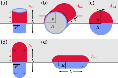
Figure 5: Shapes considered here: cylinders in (a) normal orientation (rocket mode) and (b) parallel orientation (submarine mode), (c) spherical particles, spherocylinders in (d) normal orientation and (e) parallel orientation. In a deterministic model, the particle/virus is homogeneously covered with ligands (blue) that can adhere to the cell membrane. The adhered area $A_{\mathrm{ad}}$ is marked in red.

III Deterministic dynamics

III.1 Dynamical equations

We now discuss the deterministic dynamics of adhesion-mediated particle uptake, with a focus on the role of particle shape, which next to size is the particle feature of largest interest Vácha et al. (2011); Huang et al. (2013); Dasgupta et al. (2014); Bahrami et al. (2014); Deng et al. (2019). The focus of this section is an analytical treatment of the dynamics and therefore here we include the effect of the free membrane only on the level of a line tension. Our reference shape is always the spherical one due to the dominance of icosahedral viruses. Cylindrical particles may make contact to the cell membrane at any orientation. However, a short (long) cylinder would position itself normal (parallel) to the membrane to maximize the initial adhered contact area. It is therefore reasonable to compare these two configurations (orientation normal and parallel) to the spherical (icosahedral) shape. We note that for simplicity here we neglect the top and bottom faces of the cylindrical shape and the bending energy of the kinked edges. In order to study the effect of the edges, we also consider spherocylindrical particles in normal and parallel orientation (Fig. 5). While our approach is well suited for all these shapes which obey axial symmetry, more complex shapes as for example cubes have to be investigated numerically Dasgupta et al. (2014).

During uptake the particle adheres to the membrane along the adhesive area $A_{\mathrm{ad}}$. We describe the progress of uptake by the uptake height $z$ for the normal cylinder, see Fig. 5(a), or by the uptake angle $\theta$ for the parallel cylinder or sphere, see Fig. 5(b), (c). One can calculate the thermodynamic uptake force by taking the variation of the energy $E$ with respect to the uptake variable

$$F_{\mathrm{up}}=-\partial E/\partial x,$$ (10)

where $x=z$ or $x=\theta R$. The uptake force is balanced by a friction force, $F_{\mathrm{up}}=F_{\mathrm{friction}}$. Here we assume that the dynamics of the uptake process is dominated by one local timescale. As a lower limit to all possible choices, we identify the microviscosity $\eta$ of the membrane, which is known to dominate uptake times for vesicles and which has a typical value $\eta=1\ {\rm Pa\;s}$ Agudo-Canalejo and Lipowsky (2015). Hence

$$F_{\mathrm{friction}}=\eta\mathcal{E}(x)\dot{x}.$$ (11)

Particle shape will enter our results through the variable edge length $\mathcal{E}(x)$. If one was interested in another rate-limiting dissipative process for uptake that was also dominated by one single local time scale acting at the interface between the adhered and free membrane parts, one could simply rescale all our results to the desired scale. This however would not change the relative sequence of uptake and the phase diagrams presented below. Solving the force balance equation for $\dot{x}$, we obtain the dynamic equation for particle uptake. In the next paragraphs we briefly summarise the results for the two cylinder orientations, the sphere and the two spherocylinder orientations.

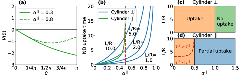
Figure 6: Cylindrical uptake. (a) Shape of the uptake potential for parallel orientation of the cylinder. Full uptake is possible for reduced membrane tension $\alpha^{\parallel}<1/2$ (uptake angle $\theta=\pi$ is a boundary minimum, green solid curve). For $\alpha^{\parallel}>1/2$, only partial uptake can take place (minimum for finite uptake angle $\theta<\pi$, green dashed). (b) Non-dimensionalised uptake times of parallel (green) and normal cylinder (blue) as a function of $\alpha^{\mathrm{\parallel}}$ at equal radius but different aspect ratios (i.e. different volume). For the normal cylinder the uptake time increases with aspect ratio whereas it stays constant for the parallel cylinder. (c) Dynamical state diagram of normal cylindrical uptake. Orange region: full uptake, green region: no uptake. (d) Dynamical state diagram of parallel cylindrical uptake. Orange region: full uptake, blue region: partial uptake. Above the dashed red line the parallel cylinder and below the dashed red line the normal cylinder is taken up fastest.

III.2 Cylinder with normal orientation $(\bot)$

For a cylinder (radius $R$, length $L$) oriented normally to the membrane one has adhesive area $A_{\mathrm{ad}}^{\bot}=\mathcal{E}^{\bot}z$, edge length $\mathcal{E}^{\mathrm{\bot}}=2\pi R$ and mean curvature $H^{\bot}=1/(2R)$, hence

$$E^{\bot}=-W2\pi Rz+\kappa\frac{\pi z}{R}+\sigma 2\pi Rz+\zeta 2\pi R.$$ (12)

We again note that the top and bottom surfaces of the cylinder would not contribute to the uptake force and are neglected here for simplicity. The differential equation for the uptake then simply reads

$$\dot{z}=-\frac{\partial E^{\bot}/\partial z}{\eta\mathcal{E}^{\bot}}.$$ (13)

One sees that the line tension does not affect the uptake dynamics as the length of the edge does not change with $z$. Thus the uptake rate is a constant, $\dot{z}=\nu_{\mathrm{up}}^{\bot}$, with

$$\nu_{\mathrm{up}}^{\bot}=\nu_{\mathrm{w}}^{\bot}-\nu_{\mathrm{\kappa}}^{\bot}-\nu_{\mathrm{\sigma}}^{\bot}=W/\eta-\kappa/(2R^{2}\eta)-\sigma/\eta.$$ (14)

In case $\nu_{\mathrm{w}}^{\bot}$ overcomes the counteracting terms $\nu_{\mathrm{\kappa}}^{\bot}+\nu_{\mathrm{\sigma}}^{\bot}$ from bending and tension, uptake progresses at constant speed and the uptake time is given by $T_{\mathrm{det}}^{\bot}=L/\nu_{\mathrm{up}}^{\bot}$. Otherwise, the particle does not get taken up at all ($\nu_{\mathrm{up}}^{\bot}\leq 0$). Partial uptake will never occur. The critical radius (at which the uptake time diverges) is given by $R_{\mathrm{crit}}^{\bot}=\sqrt{\kappa/(2(W-\sigma))}.$ The optimal radius (for which uptake is fastest) is given by $R_{\mathrm{*}}^{\bot}=\sqrt{3}R_{\mathrm{crit}}^{\bot}.$

Below we will compare all particle shapes at equal volume and equal radius because it is a natural question to ask which shape performs best at a given volume of transported cargo. Taking the sphere as the reference shape, the normally oriented cylinder then has a length $L=4R/3$.

III.3 Cylinder with parallel orientation $(\parallel)$

Completely analogously, one obtains the energy for the parallel cylinder, now as a function of the uptake angle (see Fig. 5(b))

$$E^{\parallel}=-W\theta 2LR+\kappa\frac{\theta L}{R}+\sigma(\theta-\sin\theta)2LR+\zeta 2L\,.$$ (15)

Again the bottom and top faces of the cylinder are neglected for simplicity. Then, the dynamic equation for uptake is given by

$$\dot{\theta}=\nu_{\mathrm{up}}^{\parallel}-\nu_{\mathrm{\sigma}}^{\parallel}(1-\cos\theta),$$ (16)

where $\nu_{\mathrm{up}}^{\parallel}=\nu_{\mathrm{w}}^{\parallel}-\nu_{\mathrm{\kappa}}^{\parallel}=W/(R\eta)-\kappa/(2R^{3}\eta)$ and $\nu_{\mathrm{\sigma}}^{\parallel}=\sigma/(R\eta)$. Again, the line tension does not affect the uptake dynamics.

It is insightful to non-dimensionalize the dynamic equation by introducing the characteristic time $1/\nu_{\mathrm{up}}^{\parallel}$ to get

$$\frac{\mathrm{d}\theta}{\mathrm{d}\tau}=1-\alpha^{\parallel}(1-\cos\theta).$$ (17)

We will assume $\nu_{\mathrm{w}}^{\parallel}>\nu_{\mathrm{\kappa}}^{\parallel}$ (since otherwise there is no uptake anyways) and hence the reduced membrane tension

$$\alpha^{\parallel}=\nu_{\sigma}^{\parallel}/\nu_{\mathrm{up}}^{\parallel}=\frac{2\sigma R^{2}}{2WR^{2}-\kappa}$$ (18)

is positive and uptake is expected to be the faster the smaller $\alpha^{\parallel}$ is. Eq. (17) can be integrated analytically with initial condition $\theta(t=0)=0$ to obtain $\theta(t)$. It is, however, simpler, to write it in potential form,

$$\frac{\mathrm{d}\theta}{\mathrm{d}\tau}=-\frac{dV(\theta)}{d\theta}\,\,,\,\,\,V(\theta)=-\theta+\alpha^{\parallel}(\theta-\sin\theta)\,,$$ (19)

highlighting the dynamic behaviour: first, the slope for small angles is always negative. For $0<\alpha^{\parallel}\leq 1/2$ one has a boundary minimum at $\theta=\pi$, hence complete uptake (although the uptake time diverges at $\alpha^{\parallel}=1/2$). For $\alpha^{\parallel}>1/2$ the minimum is for $\theta<\pi$ and hence one has only partial uptake, cf. Fig. 6(a). Integrating Eq. (17) leads to the uptake time

$$T_{\mathrm{det}}^{\parallel}\approx\frac{\pi}{\nu_{\mathrm{up}}^{\parallel}\sqrt{1-2\alpha^{\parallel}}}\,,$$ (20)

for $\alpha^{\parallel}<1/2$ and to the final partial wrapping angle of

$$\theta(t\rightarrow\infty)=2\arctan\left(\frac{1}{\sqrt{2\alpha^{\parallel}-1}}\right)\,,$$ (21)

for $\alpha^{\parallel}>1/2$. The critical radius is determined by $\alpha^{\parallel}=1/2$, yielding $R_{\mathrm{crit}}^{\parallel}=\sqrt{\kappa/(2(W-2\sigma))}.$

III.4 Comparison of cylinder with normal and parallel orientation

To compare the uptake times of the normally and parallelly oriented cylinders, we can express both in the reduced membrane tension $\alpha^{\parallel}$ to get

$$\frac{T^{\bot}_{\mathrm{det}}}{R\eta/\sigma}=\frac{L}{R}\frac{\alpha^{\parallel}}{1-\alpha^{\parallel}}\,\,\,,\,\,\,\frac{T^{\parallel}_{\mathrm{det}}}{R\eta/\sigma}=\pi\frac{\alpha^{\parallel}}{\sqrt{1-2\alpha^{\parallel}}}\,,$$ (22)

where $R\eta/\sigma$ is again a characteristic time scale.

Fig. 6(b) shows the rescaled uptake times for the normal (blue) and parallel cylinder (green) as a function of $\alpha^{\parallel}$ at equal radius but different aspect ratios $L/R$ (i.e. different volume). While for the parallel cylinder the uptake time is a constant, for the normally oriented cylinder it naturally increases with length and hence the aspect ratio. Consequently, the normal cylinder is faster only as long as it is rather short, explicitly as long as

$$\frac{L}{R}\leq\pi\frac{1-\alpha^{\parallel}}{\sqrt{1-2\alpha^{\parallel}}}\,.$$ (23)

The optimal uptake orientation of a cylinder hence depends on the aspect ratio.

Fig. 6(c) and (d) show the dynamical state diagrams for normal and parallel cylinder uptake as a function of aspect ratio and $\alpha^{\parallel}$. While normal cylinders are either taken up completely or not at all, parallel cylinders can also be taken up partially. We note that the state diagram for the the parallel cylinder is in agreement with the one which was previously computed by Mkrtchyan and coworkers Mkrtchyan et al. (2010). In Fig. 6(d), we also investigate the speed of uptake. Below the dashed red line the normal cylinder is taken up fastest, whereas above the dashed red line the parallel cylinder is taken up fastest.

III.5 Sphere $(\circ)$

For a sphere the total energy reads

$$E^{\circ}= \left(-W2\pi R^{2}+\kappa 4\pi+\sigma\pi R^{2}(1-\cos\theta)\right)$$

$$\times(1-\cos\theta)+\zeta 2\pi R\sin\theta\,,$$ (24)

and hence the differential equation for uptake reads

$$\dot{\theta}^{\circ} =\nu_{\mathrm{up}}^{\circ}-\nu_{\sigma}^{\circ}(1-\cos\theta)-\nu_{\zeta}^{\circ}\cot{\theta}\,,$$ (25)

where we have introduced $\nu_{\mathrm{up}}^{\circ}=\nu_{\mathrm{w}}^{\circ}-\nu_{\mathrm{\kappa}}^{\circ}=W/(R\eta)-2\kappa/(R^{3}\eta)$, $\nu_{\sigma}^{\circ}=\sigma/(R\eta)$ and $\nu_{\zeta}^{\circ}=\zeta/(R^{2}\eta)$.

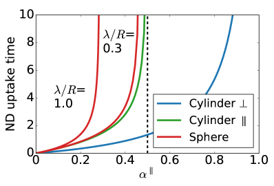
Figure 7: Non-dimensional uptake times for normal cylinder (blue), parallel cylinder (green) and sphere (red) for $\lambda/R=0.3$ and $\lambda/R=1.0$ as a function of $\alpha^{\parallel}$ and for equal volume at equal radius.

Neglecting line tension, the dynamic equation has the same form as for the parallel cylinder, albeit with different expressions for the rates. Introducing the reduced membrane tension

$$\alpha^{\circ}=\nu_{\mathrm{\sigma}}^{\circ}/\nu_{\mathrm{up}}^{\circ}=\frac{\sigma R^{2}}{WR^{2}-2\kappa}\,,$$ (26)

one hence again has for the uptake time $T_{\mathrm{det}}^{\circ}\approx\pi/(\nu_{\mathrm{up}}^{\circ}\sqrt{1-2\alpha^{\circ}})$, implying a critical radius $R_{\mathrm{crit}}^{\circ}=\sqrt{2\kappa/(W-2\sigma)}$.

To compare to the uptake times for the normal and parallel cylinder at equal volume and radius, we can again express the uptake time as a function of $\alpha^{\parallel}$ by means of

$$\alpha^{\circ}=\frac{1}{\frac{1}{\alpha^{\parallel}}-\frac{3\lambda^{2}}{2R^{2}}}\,.$$ (27)

A comparison of the uptake times of the two cylinder orientations and the sphere is shown in Fig. 7. In case of the particle being large compared to the characteristic length scale of the membrane ($\lambda/R\leq 1$, tense membrane case), the parallel cylinder and the sphere have very similar uptake times, as also evident from Eq. (27). For instance, for $\lambda/R\leq 0.1$, the uptake time for the sphere almost coincides with the green curve in Fig. 7. For smaller particles or a looser membrane, the uptake times increasingly separate, and the sphere is increasingly disfavored, as seen by the red curves in Fig. 7. In general we thus find that spheres are taken up slower than cylinders in the deterministic description Frey et al. (2019).

III.6 Spherocylinder

We now consider a spherocylindrical particle either in normal or parallel orientation with respect to the membrane. For the normal orientation the uptake time is given by the sum of the uptake times for a sphere and for a normal cylindrical particle

$$T_{\mathrm{det}}^{\,\cap}=T_{\mathrm{det}}^{\circ}+T_{\mathrm{det}}^{\bot}\,.$$ (28)

We note that at equal volume the radius of a spherocylinder ($R^{\cap}$) is always smaller compared to the radius of a sphere ($R^{\circ}$). Let us first assume that we compare a sphere and spherocylinder, which both have smaller radii compared to the optimal radius of the sphere at equal volume. In this case, it holds that $T_{\mathrm{det}}^{\,\cap}(R^{\cap})=T_{\mathrm{det}}^{\circ}(R^{\cap})+T_{\mathrm{det}}^{\bot}(R^{\cap})>T_{\mathrm{det}}^{\circ}(R^{\circ})$, since $T_{\mathrm{det}}^{\bot}(R^{\cap})>T_{\mathrm{det}}^{\circ}(R^{\circ})-T_{\mathrm{det}}^{\circ}(R^{\cap})<0$ (i.e. the uptake time of a sphere decreases below the optimal radius with increasing size).

To get insight into the general situation, we consider in Fig. 8 the uptake time as a function of volume of three normal spherocylinders (solid blue lines) with fixed but different radii. We compare the spherocylinders to a sphere with equal volume (solid red). At vanishing cylindrical length $L$ (cf. Fig. 5(d)) the uptake times of the spherocylinders and sphere are of course identical. For increasing volume, i.e. increasing cylindrical length we find that the sphere is always taken up faster compared to the normal spherocylinders. In the case when the radius and length are changed at equal volume, one moves on vertical lines through the diagram (dashed blue line). By reducing the cylindrical length, the particle radius has to increase, while keeping the volume fixed. Upon reducing the length one finally gets back onto the uptake curve of a sphere (which is of course identical to a spherocylinder with vanishing cylindrical length). Since this argument can be repeated for all radii, the spherocylinder is always taken up slower compared to the sphere at equal volume.

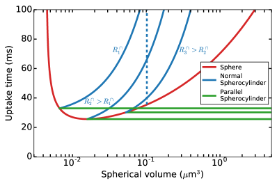
Figure 8: Uptake time as a function of spherical volume for the sphere (solid red) and spherocylinders with different radii in normal (solid blue) and parallel (solid green) orientation. The dashed blue line marks the uptake times of normal spherocylindrical particles at equal volume. Starting from the red curve, the length of the cylindrical part increases while reducing the particle radius.

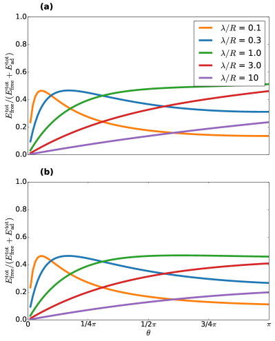
Figure 9: (a) The bending and tension energy of the free membrane of a cylindrical particle in parallel orientation relative to the total bending and tension energy, i.e. of the adhered and free parts of the membrane for different values of $\lambda/R$. (b) Similar to (a) but now for the phenomenological description of the free membrane parts.

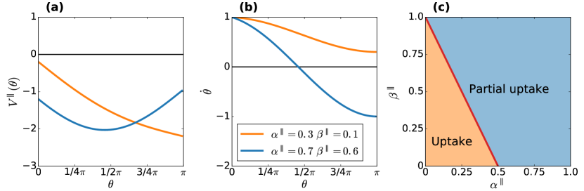
Figure 10: Deterministic uptake dynamics of a cylinder in parallel orientation including the exact solution for the free membrane. (a) Uptake potential, leading to uptake (orange) and partial uptake (blue). Parameters are given in (b). (b) Phase portrait ($\dot{\theta}$ vs. $\theta$) for different parameter values corresponding to uptake (orange) and partial uptake (blue). (c) Dynamical state diagram of the final steady states as a function of $\beta^{\parallel}$ vs. $\alpha^{\parallel}$. Below the red curve the cylinder is taken up completely (orange region) and above we find only partial uptake (blue region).

For the spherocylindrical particle in parallel orientation the uptake time is given by the slowest mode as the spherical part and the cylindrical part are taken up simultaneously. As the uptake time for the parallel cylindrical particle is always faster than the uptake time of a spherical particle at equal volume and radius the uptake time of the spherocylindrical particle in parallel orientation is given by the uptake time of the spherical particle alone

$$T_{\mathrm{det}}^{\,\supset}=T_{\mathrm{det}}^{\circ}\,.$$ (29)

Hence, the uptake time of the spherocylindrical particle in parallel orientation is constant while adapting the volume by only increasing the length of the cylindrical part. In Fig. 8 the uptake times for a spherocylindrical particles in parallel orientation with fixed but different spherical radii are shown in solid green. While for a sphere the relation between volume and radius is unambiguous, for a spherocylinder there exist different combinations of radii and lengths with the same volume. While the lowest green curve corresponds to a parallel spherocylinder with optimal spherical radius, the curve starting at smaller (larger) volume corresponds to a parallel spherocylinder with smaller (larger) radius. We see that spherical particles present clear optima in terms of uptake times at intermediate volumes, while spherocylinders are faster for large volumes, because there additional volume does not increase their uptake times when implemented by increased length.

To conclude, at equal volume a normal spherocylinder is taken up slower compared to a sphere, independent of length. For a parallel spherocylinder the order of uptake depends on the aspect ratio. For the same volume and aspect ratio parallel spherocylinders are taken up faster compared to normal spherocylinders. Comparing the uptake times of a (normal or parallel) cylinder to a (normal or parallel) spherocylinder at equal volume and radius, we find that cylinders are always taken up faster. The reason is that it is more time consuming to wrap the spherical caps compared to the cylindrical parts with the same volume.

IV State diagrams for parallel cylinder

IV.1 Free membrane energies

We now explicitly consider the effect of the free membrane. We first note that for a cylindrical particle in normal orientation, the shape equations are similar to the case of a spherical particle with $\theta=\pi/2$. However, the energy of the free membrane is a constant since it does not depend on the invagination depth $z$. Therefore, the free membrane will not contribute to the dynamics of particle uptake. The first non-trivial case therefore is the parallel cylinder. In the next section, we will then discuss the spherical particle.

For the parallel cylinder the energy of the free membrane compared to the flat case can be written as Mkrtchyan et al. (2010)

$$\frac{E_{\mathrm{free}}^{\mathrm{tot\parallel}}}{\kappa}=\frac{8L}{\lambda}\left(1-\cos\frac{\theta}{2}\right)\,.$$ (30)

Details can be found in appendix B. Considering the free membrane on both cylinder sides, the scaling of the free energy is then given by $E_{\mathrm{free}}^{\mathrm{tot\parallel}}\sim\zeta L\theta^{2}=E_{\mathrm{free}}^{\mathrm{pheno\,\parallel}}$, which is the analogous of the phenomenological approach of Eq. (9) for spheres. The energy of the free membrane relative to the energy of both the free and adhered membrane parts are shown in Fig. 9(a) for different values of $\lambda/R$. In Fig. 9(b) the same is shown for the phenomenological description. The agreement is very good and we conclude that the phenomenological approach works very well in this case.

IV.2 Dynamics with free membrane

We now study the uptake dynamics for the parallel cylinder including the free membrane. The dynamical equation in non-dimensional form reads

$$\frac{\mathrm{d}\theta}{\mathrm{d}\tau}=1-\alpha^{\parallel}(1-\cos\theta)-\beta^{\parallel}\sin{\theta/2}\,,$$ (31)

with $\tau=t\nu_{\mathrm{up}}^{\parallel}$ and the reduced line tension

$$\beta^{\parallel}=\frac{\nu_{\zeta}^{\parallel}}{\nu_{\mathrm{up}}^{\parallel}}=\frac{4\sqrt{\kappa\sigma}R}{2WR^{2}-\kappa}\;\;\;\mathrm{and}\;\;\;\nu_{\zeta}^{\parallel}=\frac{2\sqrt{\kappa\sigma}}{\eta R^{2}}\,,$$ (32)

which incorporates the effect of the free membrane. Importantly, the uptake dynamics does not depend on the length of the parallel cylinder.

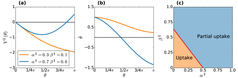
Figure 11: Deterministic uptake dynamics of a cylinder in parallel orientation including the free membrane by the phenomenological description. (a) Uptake potential for different parameter values corresponding to uptake (orange) and partial uptake (blue). (b) Phase portrait ($\dot{\theta}$ vs. $\theta$). Parameters are given in (a). (c) Dynamical state diagram of the final steady states as a function of $\beta^{\parallel}$ vs. $\alpha^{\parallel}$. Below the red curve the cylinder is taken up completely (orange region) and above we find only partial uptake (blue region).

In potential form, the dynamics $\frac{\mathrm{d}\theta}{\mathrm{d}\tau}=-\frac{dV(\theta)}{d\theta}$ follows from

$$V(\theta)=-\theta+\alpha^{\parallel}(\theta-\sin\theta)-2\beta^{\parallel}\cos\frac{\theta}{2}\,.$$ (33)

This potential is shown in Fig. 10(a). One either has a boundary minimum corresponding to full uptake (orange) or a minimum in between corresponding to partial uptake (blue), depending on the parameter choice. From the shape of the potential and the phase portrait in Fig. 10(b) we can deduce the dynamical state diagram of uptake in the $\beta^{\parallel}$-$\alpha^{\parallel}$-plane in Fig. 10(c) for a parallel cylinder. We find that the parallel cylinder either gets taken up completely (orange) or only partially (blue). The boundary between these two states is given when Eq. (31) becomes zero. As the second and third term in Eq. (31) become minimal for $\theta=\pi$, we find the boundary between the partial and full uptake state when

$$\frac{\mathrm{d}\theta}{\mathrm{d}\tau}\bigg{|}_{\theta^{\parallel}=\pi}=0\rightarrow\beta^{\parallel}=1-2\alpha^{\parallel}\,.$$ (34)

IV.3 Dynamics with phenomenological approach

We now consider the phenomenological ansatz adapted to the case of a parallel cylinder. In general, the energy of the phenomenological approach can be written as $E_{\mathrm{free}}^{\mathrm{pheno}}=1/2\zeta\theta^{2}\mathcal{E}$, where $\mathcal{E}$ is the length of the line that connects the adhered membrane and the free membrane. For the parallel cylinder we have $\mathcal{E}^{\parallel}=2L$ and thus $E_{\mathrm{free}}^{\mathrm{pheno\,\parallel}}=\zeta L\theta^{2}$, where $\zeta=\sqrt{\kappa\sigma}$. The dynamics for the phenomenological approach is then given by

$$\frac{\mathrm{d}\theta_{\mathrm{pheno}}}{\mathrm{d}\tau}=1-\alpha^{\parallel}(1-\cos\theta)-\frac{\beta^{\parallel}}{2}\theta\,.$$ (35)

In potential form, the dynamics now reads

$$V_{\mathrm{pheno}}(\theta)=-\theta+\alpha^{\parallel}(\theta-\sin\theta)+\frac{\beta^{\parallel}}{4}\theta^{2}\,.$$ (36)

The boundary between these two states is given when Eq. (35) becomes zero. As the second term in Eq. (35) becomes minimal for $\theta=\pi$ we find

$$\frac{\mathrm{d}\theta_{\mathrm{pheno}}}{\mathrm{d}\tau}\bigg{|}_{\theta^{\parallel}=\pi}=0\rightarrow\beta^{\parallel}=\frac{2-4\alpha^{\parallel}}{\pi}\ .$$ (37)

The potential in Fig. 11(a), the uptake dynamics in Fig. 11(b) and the state diagram of uptake in Fig. 11(c) for the dynamics in the phenomenological description can be easily compared to the exact case of the free membrane in Fig. 10. We see that the dynamics are very similar.

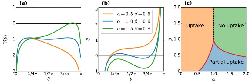
Figure 12: Deterministic uptake dynamics of spherical particles with line tension. (a) Uptake potential, leading to uptake (orange), partial uptake (blue) and no uptake (green). Parameters are given in (b). (b) Phase portrait ($\dot{\theta}$ vs. $\theta$) for different parameter values corresponding to uptake (orange), partial uptake (blue) and no uptake (green). (c) Dynamical state diagram of the final steady states as a function of $\beta$ vs. $\alpha$. Below the red curve the sphere is taken up only partially (blue region) and above we find either uptake (orange region) or no uptake (green region).

V State diagrams for sphere

V.1 Line tension

We now study the uptake dynamics for the sphere by including the free membrane by a line tension or by a phenomenological ansatz. We first consider a line tension. The dynamical equation in non-dimensional form reads

$$\frac{\mathrm{d}\theta}{\mathrm{d}\tau}=1-\alpha(1-\cos\theta)-\beta\cot{\theta}\,,$$ (38)

with $\tau=t\nu_{\mathrm{up}}^{\circ}$ and the reduced line tension

$$\beta=\nu_{\zeta}^{\circ}/\nu_{\mathrm{up}}^{\circ}=\frac{\zeta R}{WR^{2}-2\kappa}\,,$$ (39)

and the reduced surface tension $\alpha=\alpha^{\circ}$ as before. In potential form, the dynamics reads $\frac{\mathrm{d}\theta}{\mathrm{d}\tau}=-\frac{dV(\theta)}{d\theta}$, now with

$$V(\theta)=-\theta+\alpha(\theta-\sin\theta)+\beta\ln(\sin\theta)\,.$$ (40)

From the shape of the potential, visualized in Fig. 12(a), one can clearly see that the line tension creates divergences towards $-\infty$ for both $\theta=0$ and $\theta=\pi$. The divergence at small $\theta$ is well known from classical nucleation theory and implies that a fluctuation is required to start the process. The divergence at large $\theta$ reflects the fact that a line tension accelerates the process once the equator is passed.

Since the potential varies between $-\infty$ and $-\infty$ for $0\leq\theta\leq\pi$, it must have at least one maximum, corresponding to an unstable steady state. In case this is the only steady state, we now assume that the initial fluctuations bring the system over the initial barrier and the result will be full uptake. However, as a function of reduced membrane and line tension $\alpha$ and $\beta$, additional extrema in the potential and hence additional steady states can emerge. We identify two scenarios. If the potential displays two maxima separated by a minimum, then we have another steady state that we interpret as partial uptake. If the potential displays a saddle for values of $\theta$ smaller then those for the maximum, then we conclude that no uptake is possible since $\dot{\theta}<0$ except for very large $\theta$. Fig. 12 visualizes our three scenarios for the dynamics both via the potential (a) and using the phase portrait $\dot{\theta}$ vs. $\theta$ (b).

The steady states of Eq. (38) as a function of $\alpha$ and $\beta$ can be studied analytically. In fact, their number can change only if the curvature of a given stationary point changes sign. One can reformulate the problem to find the particular value of $\beta$ where the two functions $f(\theta_{\mathrm{ss}})=1-\alpha(1-\cos\theta_{\mathrm{ss}})$ and $g(\theta_{\mathrm{ss}})=\beta\cot\theta_{\mathrm{ss}}$ are equal, $f(\theta_{\mathrm{ss}})=g(\theta_{\mathrm{ss}})$ (defining a steady state), and where their derivatives are equal, $f^{\prime}(\theta_{\mathrm{ss}})=g^{\prime}(\theta_{\mathrm{ss}})$ (defining the change in the sign of the curvature). The second condition implies that $\sin^{3}\theta_{\mathrm{ss}}=\beta/\alpha$ and insertion into the first equation results in

$$\beta(\alpha)=\alpha\left[1-\left(\frac{1}{\alpha}-1\right)^{\frac{2}{3}}\right]^{\frac{3}{2}}.$$ (41)

Fig. 12(c) shows the dynamical state diagram for the uptake of a sphere in the $\beta$-$\alpha$-plane. Eq. (41) is shown as the red curves. Below these curves one has partial uptake (blue region) and above we find either uptake (orange region) or no uptake (green region), according to the definition discussed above. Note that the red curve tends to $\alpha=1/2$ for $\beta\rightarrow 0$, as expected.

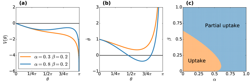
Figure 13: Deterministic uptake dynamics of spherical particles with the phenomenological contribution of the free membrane. (a) Uptake potential, leading to uptake (orange) and partial uptake (blue). (b) Phase portrait ($\dot{\theta}$ vs. $\theta$) for different parameter values corresponding to uptake (orange) and partial uptake (blue). Parameters as in (a). (c) Dynamical state diagram of the final uptake states as a function of $\beta$ vs. $\alpha$. Full uptake is achieved in the orange region and partial uptake in the blue region.

Interestingly, a moderate reduced line tension $\beta$ is productive as it increases the range of reduced membrane tension $\alpha$ for which full uptake occurs. This effect however saturates at $\beta=1$. Stronger values of $\beta$ are counter-productive as they transform partial uptake into no uptake. We note that for typical parameter values (using $\zeta=\sqrt{\kappa\sigma}$, i.e. assuming that the line tension is a result of the free membrane effects) one estimates $\alpha=0.5$ and $\beta=0.5$, for which one would expect uptake.

In general, since the uptake dynamics depends on four parameters ($R$, $W$, $\kappa$ and $\sigma$) and $\alpha$ and $\beta$ are combinations of those, one would not move along horizontal or vertical lines in an experiment, where typically only one parameter is varied. However, since $\beta/\alpha=\lambda/R$ one could move on straight lines through the origin in the phase diagram when changing $W$ while keeping $\lambda/R$ constant.

V.2 Phenomenological description

We now discuss the case when the simple line tension, Eq. (7), is replaced by the phenomenological description, Eq. (9), distilled out from the shape equations. The additional factor of $\theta^{2}/2$ in Eq. (9) versus Eq. (7) results in the dynamical equation

$$\frac{\mathrm{d}\theta}{\mathrm{d}\tau}=1-\alpha(1-\cos\theta)-\beta\theta\left(1+\frac{1}{2}\theta\cot{\theta}\right)\,,$$ (42)

with the same reduced membrane tension $\alpha$ and reduced line tension $\beta$ as before. Now the last term cannot be integrated in closed analytical form as before. The potential can be, however, easily obtained numerically as displayed in Fig. 13(a). One clearly sees that the divergence at $\theta=0$, as occurring for the line tension, is now absent while the speed-up of uptake for large angle persists. Now only full uptake (orange) and partial uptake (blue) can be observed. However, we note that a trivial no uptake state occurs for insufficient adhesion energy. Fig. 13(b) shows the phase portrait and (c) the dynamical state diagram for the uptake in the $\beta$-$\alpha$-plane. Interestingly, the latter displays a re-entrance phenomenon at $\alpha$-values slightly above $1/2$, meaning that upon increasing $\beta$ the system can display partial uptake, full uptake and again partial uptake. We note that the re-entrance phenomenon could be potentially observed when changing R while keeping $W$, $\sigma$ and $\kappa$ constant.

Let us now compare and discuss the cases of no line tension vs. line tension vs. the phenomenological treatment of the free membrane. We will take a dynamical systems point of view, which turns out to be especially instructive. Fig. 14 shows the steady states as a function of the reduced membrane tension $\alpha$, for the three cases. As shown in Fig. 14(a), without line tension ($\beta=0$) the dynamics is quite simple: for $\alpha<1/2$ (i.e. small reduced membrane tension), full uptake is achieved as $\theta=\pi$ is the only attractor. As soon as $\alpha>1/2$ (i.e. intermediate reduced membrane tension), this only attractor moves to finite angles $\theta_{ss}<\pi$, corresponding to partial uptake, decreasing further with increasing $\alpha$. The arrows mark the flow of the system, towards the stable attractors. Starting from the first adhesion formed, corresponding to $\theta=0$, the system hence always evolves towards full or partial uptake, depending on reduced membrane tension $\alpha$.

The reduced line tension, as visible in Fig. 14(b), has two main effects: first, $\theta=0$ becomes a steady state, due to the divergence of the potential. Second, another steady state emerges at intermediate angle, which has unstable (dashed) parts, but also a stable (solid) region corresponding to partial uptake. The bifurcation structure is the one of a pair of saddle-nodes. While one assumes that the unstable branch for low reduced membrane tension $\alpha$ can be overcome by the inherent fluctuations in receptor-ligand bond formation, hence still leading to full uptake, the unstable branch for large reduced membrane tension $\alpha$ is at such a large angle that it should be interpreted as no possible uptake. Finally, the stable branch in between the two saddle-nodes corresponds to the attractor of partial uptake.

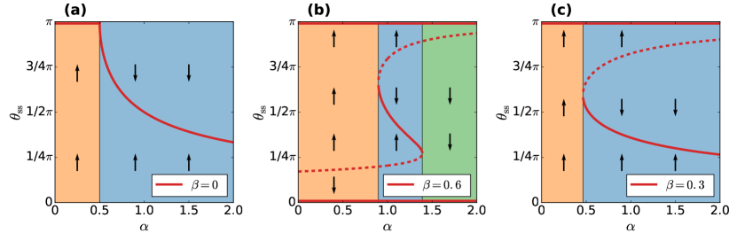
Figure 14: Steady states as a function of the reduced membrane tension $\alpha$, in case of (a) no line tension ($\beta=0$), (b) for a line tension with $\beta=0.6$ and (c) including the phenomenological description of the free membrane, Eq. (9), for $\beta=0.3$. Stable steady states are marked in solid, unstable ones as dashed. The arrows display the flow of the system. As usual, regions of full uptake are marked in orange, partial uptake in blue and no uptake in green. Note that for (a) there is only one stable steady state and the dynamics is simple. Line tension (b) and the free membrane effects (c) introduce new steady states undergoing saddle-node bifurcations (see text).

Figure 15: Steady states for line tension/free membrane effects as a function of reduced line tension $\beta$. Stable steady states are marked in solid, unstable ones as dashed. The arrows display the flow of the system. As usual, regions of full uptake are marked in orange and partial uptake in blue. (a) Case of line tension and $\alpha=0.8$. The partial uptake for small $\beta$ is due to the saddle-node, whose stable branch prevents the system from reaching full uptake. Increasing $\beta$ (and assuming the unstable branch can be overcome by fluctuations) induces full uptake. (b) Phenomenological treatment for the free membrane with $\alpha=0.6$. Here, the system displays partial uptake, full uptake and again partial uptake, i.e. a “re-entrance” of partial uptake occurs. (c) Same as (b) but for $\alpha=0.8$ showing only partial uptake for increasing $\beta$.

Using the phenomenological description of the free membrane effects leads to the scenario shown in Fig. 14(c). Here, the ambiguity of overcoming a barrier at small angle is absent, as $\theta=0$ is not a steady state anymore and no other branch prevents the flow from reaching $\theta=\pi$. Only a single saddle-node emerges for larger reduced membrane tension $\alpha$, separating uptake from partial uptake. In a certain sense, the phenomenological description is an intermediate case between having no line tension and a simple line tension.

Fig. 15 shows the dynamics and the dependence of the steady states on the reduced line tension $\beta$, describing the strength of the line tension (a) or free membrane effects (b), (c), respectively. One can clearly see that the emergence of saddle-nodes (one of whose branches has to be stable) directly corresponds to the regions of partial uptake. Fig. 15(b) shows an example of the re-entrance phenomenon, i.e. where partial uptake emerges twice when varying the parameter $\beta$, cf. also Fig. 13(c).

To conclude, both a line tension and the approximated free membrane effects considerably enrich the uptake dynamics. They share similarities, for instance they accelerate uptake as soon as the circumference of the membrane edge decreases, i.e. in the second half of uptake ($\theta>\pi/2)$. Although a partial uptake state can exist alone due to the interplay of adhesion energy and membrane tension that can generate a boundary minimum of the potential for spherical particles, here another partial uptake state can emerge. This partial uptake state is caused by a non-boundary minimum of the potential due to the saddle-node structures of the new steady states that is generated either by line tension or approximated free membrane effects. While the line tension can introduce no uptake states that are caused if a repellor at large angle values emerges, no uptake states only emerge in the phenomenological description in the trivial case of insufficient adhesion energy. The main difference between them, however, is that the line tension introduces an energy barrier at small angles, that has to be overcome by fluctuations. Therefore a line tension is not an adequate description for the free membrane, which does not show this effect. We stress that this conclusion remains true beyond the approximation used in Eq. (9): Eq. (53) leads to $E_{\mathrm{free}}^{\mathrm{tot}}\propto\sin^{4}\theta$ for small angles, displaying the same behavior, i.e. no barrier.

VI Stochastic dynamics

VI.1 General approach

For the uptake of both nanoparticles or viruses, fluctuations are expected to be important since the particles are small and typically only covered by few tens of ligands, rendering ligand-receptor binding a discrete stochastic process. Based on the continuous deterministic modeling approach, we now explicitly model the discrete stochastic dynamics of receptor-ligand binding as sketched schematically in Fig. 16. Our stochastic model is defined from the deterministic one via two steps. First, the system is discretized by mapping the continuous deterministic equation onto a discretized version. Secondly, this equation is interpreted as a stochastic rate equation. The considered stochastic process is designed to obtain the deterministic result in the limit of small noise, i.e. in the continuous deterministic limit. However, we do not introduce temperature and our stochastic model is not designed to obtain the deterministic result in the limit of vanishing temperature. The underlying reason is that we do not want to make assumptions about the processes that drive the membrane forward and backward. Modelling the growth of adhered membrane patches based on receptor-ligand binding is a mature and challenging field by itself Reister-Gottfried et al. (2008); Weikl et al. (2009) and might even include active processes Turlier et al. (2016). Therefore we do not anchor our model in an equilibrium model, but derive our stochastic rates from the deterministic theory without enforcing detailed balance, similar to stochastic processes used in population or evolutionary dynamics Cremer et al. (2012); Melbinger et al. (2010).

In detail, we first map the adhered membrane area onto the number of bound ligands $N$, in order to deduce a discrete differential equation $\mathrm{d}N/\mathrm{d}t=\mathrm{d}N/\mathrm{d}x\cdot\mathrm{d}x/\mathrm{d}t$, where $x=\{z,\theta\}$ corresponds to the uptake variable (height $z$ for the cylinder in normal orientation and invagination angle $\theta$ for the parallel cylinder and the sphere) Frey et al. (2019). From the deterministic framework, $\mathrm{d}x/\mathrm{d}t$ is known from Eq. (13), Eq. (16) and Eq. (25) for normal cylinders, parallel cylinders and spheres, respectively. The next step is to deduce the corresponding one-step Master equation (ME) Van Kampen (1992) for the probability $p_{N}$ to have $N$ ligands bound to receptors,

$$\frac{\mathrm{d}p_{N}}{\mathrm{d}\tau}=g_{N-1}p_{N-1}+r_{N+1}p_{N+1}-(g_{N}+r_{N})p_{N}.$$ (43)

Here $g_{N}$ is the forwards and $r_{N}$ the backwards rate by which ligands bind (unbind) from state $N$. While complete probability distributions can be calculated analytically only for some special cases, the stochastic uptake times $T_{\mathrm{sto}}$ for a reflecting boundary at the unwrapped state and an absorbing boundary at the fully wrapped state can be calculated analytically as Van Kampen (1992)

$$T_{\mathrm{sto}}=\sum_{\nu=1}^{N_{\mathrm{max}}-1}\sum_{\mu=1}^{\nu}\frac{r_{\nu}r_{\nu-1}\cdot\cdot\cdot r_{\mu+1}}{g_{\nu}g_{\nu-1}\cdot\cdot\cdot g_{\mu}}\,.$$ (44)

Alternatively, one can use the Gillespie algorithm Gillespie (1977) to simulate both the probability distributions and the uptake times.

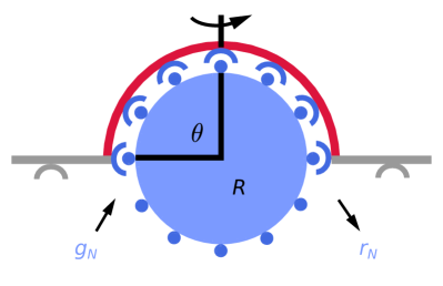
Figure 16: Modeling particle uptake as a discrete stochastic process. The particle (blue) is covered with ligands (small discs) that stochastically bind to cell surface receptors (half-circles) with rate $g_{N}$, leading to an advancement of the adhered membrane area, or unbind with rate $r_{N}$. Note that axial symmetry is assumed.

VI.2 Cylinder with normal orientation $(\bot)$

For a cylinder oriented perpendicularly to the membrane, the membrane covered area $A_{\mathrm{ad}}^{\bot}=A(z)$ is mapped onto the number of bound receptors $N^{\bot}(z)$ by using

$$A(z)/A_{\mathrm{max}}^{\bot}=(N^{\bot}(z)-1)/(N_{\mathrm{max}}-1).$$ (45)

Here we assumed that initially, the particle is already bound to the membrane by one ligand, yielding $N^{\bot}(z)=(N_{\mathrm{max}}-1)z/L+1$. The corresponding discrete equation then reads

$$\frac{\mathrm{d}N^{\bot}}{\mathrm{d}t}=\frac{N_{\mathrm{max}}-1}{L}\left(\nu_{\mathrm{w}}^{\bot}-\nu_{\mathrm{\kappa}}^{\bot}-\nu_{\mathrm{\sigma}}^{\bot}\right)\,,$$ (46)

and the corresponding rates of the ME are hence easily deduced by $g_{N}=(N_{\mathrm{max}}-1)\nu_{\mathrm{w}}^{\bot}/L$ and $r_{N}=(N_{\mathrm{max}}-1)(\nu_{\mathrm{\kappa}}^{\bot}+\nu_{\mathrm{\sigma}}^{\bot})/L$. Finally, to implement a reflecting boundary condition at $N=1$, we put $r_{1}$=0.

VI.3 Cylinder with parallel orientation $(\parallel)$

In this case we proceed similarly and map the membrane covered area $A_{\mathrm{ad}}^{\parallel}=A(\theta)$ onto the number of bound receptors $N^{\parallel}(\theta)$ via $A(\theta)/A_{\mathrm{max}}^{\parallel}=(N^{\parallel}(\theta)-1)/(N_{\mathrm{max}}-1)$. One intitially bound ligand implies $N^{\parallel}(\theta)=(N_{\mathrm{max}}-1)\theta/\pi+1$. The corresponding discrete equation reads

$$\frac{\mathrm{d}N^{\parallel}}{\mathrm{d}t}=\frac{N_{\mathrm{max}}-1}{\pi}\left(\nu_{\mathrm{w}}^{\parallel}-\nu_{\mathrm{\kappa}}^{\parallel}-\nu_{\mathrm{\sigma}}^{\parallel}(1-\cos\theta)\right)\,,$$ (47)

and hence the corresponding rates of the ME amount to $g_{N}=(N_{\mathrm{max}}-1)\nu_{\mathrm{w}}^{\parallel}/\pi$ and $r_{N}=(N_{\mathrm{max}}-1)(\nu_{\mathrm{\kappa}}^{\parallel}+\nu_{\mathrm{\sigma}}^{\parallel}(1-\cos\theta))/\pi$. Finally, to implement a reflecting boundary condition at $N=1$, we again put $r_{1}$=0.

VI.4 Sphere $(\circ)$

Finally, for a spherical particle we map $A_{\mathrm{ad}}^{\circ}=A(z)$ onto $N^{\circ}(\theta)$ by

$$A(\theta)/A_{\mathrm{max}}^{\circ}=(N^{\circ}(\theta)-1)/(N_{\mathrm{max}}-1)\,,$$ (48)

and one initially bound ligand implies $N^{\circ}=(N_{\mathrm{max}}-1)(1-\cos(\theta))/2+1$. The discrete equation reads

$$\frac{\mathrm{d}N^{\circ}}{\mathrm{d}t}=\left(\nu_{\mathrm{w}}^{\circ}-\nu_{\kappa}^{\circ}-\nu_{\sigma}^{\circ}(1-\cos\theta)-\nu_{\zeta}^{\circ}\cot{\theta}\right)N_{\mathcal{E}}(N).$$ (49)

Here $N_{\mathcal{E}}(N)=\sqrt{(N-1)((N_{\mathrm{max}}-1)-(N-1))}$ is the number of receptors at the advancing edge. The corresponding rates of the ME are given by $g_{N}=\nu_{\mathrm{w}}^{\circ}N_{\mathcal{E}}(N)$ and $r_{N}=(\nu_{\kappa}^{\circ}+\nu_{\sigma}^{\circ}(1-\cos\theta)+\nu_{\zeta}^{\circ}\cot{\theta})N_{\mathcal{E}}(N)$ for $\theta<\pi/2$ and $g_{N}=(\nu_{\mathrm{w}}^{\circ}-\nu_{\zeta}^{\circ}\cot{\theta})N_{\mathcal{E}}(N)$ and $r_{N}=\left(\nu_{\kappa}^{\circ}+\nu_{\sigma}^{\circ}(1-\cos\theta)\right)N_{\mathcal{E}}(N)$ for $\theta\geq\pi/2$ in order to ensure that the rates stay positive. In case of the phenomenological treatment of the free membrane parts, the last term in the bracket of $r_{N}$ and $g_{N}$ is replaced by $\nu_{\zeta}^{\circ}\,\theta(1+\theta/2\cot{\theta})$ in the intervals $\theta<2.289$ and $\theta\geq 2.289$, accordingly.

Finally, note that in case of the sphere one has to make additional assumptions for the rate $g_{1}$, which otherwise would be zero. We here choose $g_{1}=\nu_{\mathrm{w}}^{\circ}\sqrt{N_{\mathrm{max}}}$, since (i) it should be proportional to $\nu_{w}$ and (ii) the transition time from state $N=1$ to state $N=2$ should vanish for large $N_{\mathrm{max}}$. Since $r_{1}=0$, $N=1$ is a reflecting pure boundary, i.e. a particle always stays attached to the membrane.

Table 1: Simulation parameters.

Parameter	Used value	Ref.
Bending rigidity	$\kappa=25\,\mathrm{k_{B}}T$	Kumar and Sain (2016)
Membrane tension	$\sigma=1\cdot 10^{-5}\,\rm N/m$	Foret (2014)
Energy density	$W=0.04\,\rm{mJ/m^{2}}$	Agudo-Canalejo and Lipowsky (2015)
Membrane microviscosity	$\eta=1\,\rm Pa\;s$	Agudo-Canalejo and Lipowsky (2015)
Line tension	$\zeta=\sqrt{\kappa\sigma}$
Receptor-ligand pairs	$N_{\mathrm{max}}=20$

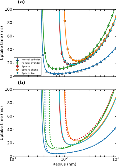
Figure 17: (a) Simulated mean uptake times (symbols) for a normally oriented cylinder (blue triangles), a parallelly oriented cylinder (green lozenges), a sphere (red circles), a sphere including the phenomenological approximation for the free membrane (orange pentagons) and a sphere with line tension (cyan stars) as function of radius at equal volume and radius for the parameter values in Table 1. In addition, the numerically computed mean uptake times calculated by Eq. (44) are shown as solid lines for the different shapes in the corresponding colors. (b) For the normal cylinder, the parallel cylinder and the sphere the deterministic uptake times are shown as dashed lines in corresponding colors (for vanishing line tension/free membrane) and compared to the numerically calculated mean uptake times (solid lines).

VI.5 Stochastic uptake times

We numerically solve the MEs corresponding to the different particle shapes and orientations by means of the Gillespie algorithm Gillespie (1977). The used parameter values are summarized in Table 1. For the number of ligands we chose a typical value of $N_{\mathrm{max}}=20$. Stochastic effects further increase upon decreasing $N_{\mathrm{max}}$, and they prevail for $N_{\mathrm{max}}$ of the order of one hundred Frey et al. (2019), depending on parameters.

In order to obtain the stochastic uptake times, we introduce an absorbing boundary at full coverage. Fig. 17(a) shows the uptake time as a function of the radius of the particle. The results of our simulations (symbols), averaged over $10^{4}$ trajectories each, perfectly agree with the results of the numerical calculations by means of Eq. (44) (solid lines), which verifies our simulations. To compare cylinders to spheres, their radius were fixed to the one of the respective sphere and the length $L$ was adjusted to obtain equal volume. Shown in the figure are the mean uptake times obtained by stochastic simulations (averaged over $10^{4}$ trajectories each) for the normally oriented cylinder (blue triangles), the parallelly oriented cylinder (green lozenges), the sphere (red circles), the sphere including the phenomenological treatment of the free membrane, according to Eq. (8) and Eq. (9) (orange pentagons) and the sphere including a line tension (cyan stars), according to Eq. (7) and Eq. (8).

In Fig. 17(b) the mean uptake times obtained by numerical calculations for the different particle shapes are compared to the deterministic results (without line tension or free membrane effects), which are shown as the dashed curves in the corresponding colors. We see that for all considered particle shapes both the deterministic and the stochastic dynamics show similar behavior. First, a critical radius exists below which uptake is not possible anymore (cf. the analytical results in section III B,C,D) Lipowsky and Döbereiner (1998). Second, for larger radii the uptake time increases with increasing particle size. And third, in between an optimal radius exists, having minimal uptake time Osaki et al. (2004); Gao et al. (2005); Zhang et al. (2009); Huang et al. (2013). The underlying reason for this behavior is that the bending energy is independent of particle size, while the energy contributions for adhesion and tension increase with size Lipowsky and Döbereiner (1998).

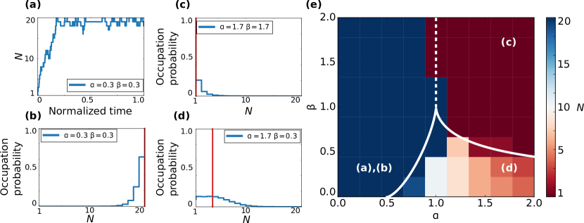
Figure 18: Stochastic uptake dynamics of spherical particles with line tension. (a) Uptake trajectory of a spherical particle with $\alpha=0.3$ and $\beta=0.3$ for $N=10^{2}$ time steps. (b)-(d) Occupation probability during uptake with $N_{\mathrm{max}}=20$ receptors for different parameter combinations for an uptake trajectory of $N=10^{6}$ time steps. The receptor with largest occupation probability is shown in red. (b) Uptake. (c) No uptake. (d) Partial uptake. (e) Dynamical state diagram of stochastic uptake showing the maximum occupation probability of a trajectory of $N=10^{6}$ time steps. The white lines correspond to the state boundaries of the deterministic model, cf. Fig. 12(c).

From Fig. 17 we further see that stochastic uptake is always faster than deterministic uptake. In addition, stochasticity extends uptake towards regions beyond the critical radius of deterministic uptake. This is due to fluctuations being able to drive particles above energy barriers during uptake. Another interesting observation is that in the deterministic description, cylinders in the parallel orientation are taken up faster than (or at least equally fast as) spherical particles for all radii. In contrast, the stochastic description states that parallelly oriented cylinders are only faster than spheres below a certain radius: for the given parameters, at around $R=150\,{\rm nm}$, the situation reverses and spheres are taken up faster Frey et al. (2019). In addition, we note that the typical time scale for uptake is between a few ms to a few tens of ms, which is in agreement with previous simulation results Huang et al. (2013).

We now discuss the effects of the line tension and the free membrane. As can be judged from Fig. 17(a) when comparing red circles, orange pentagons and cyan stars, when a line tension is used to model the free membrane parts Lipowsky and Döbereiner (1998), suggesting the scaling $\zeta=\sqrt{\kappa\sigma}$ Deserno (2004), or when incorporating the phenomenological approximation given by Eq. (8) and Eq. (9), the effects are relatively modest in regard to the uptake times. One nevertheless can see that the line tension slightly hinders uptake, while the phenomenological treatment slows down the uptake of small particles even more. For increasing particle sizes the effect vanishes as $\nu_{\zeta}\sim 1/R^{2}$. Furthermore, as the effect of the free membrane only slightly affects uptake times and contributes up to $20\%$ to the total deformation energy of the membrane, neglecting the free membrane as done in Ref. Frey et al. (2019) is justified in regard to uptake times and for typical parameters for nanoparticle and virus uptake. However, a line tension can also originate from a localization of lipids or curvature generating proteins at the border between adhered and free membrane Lipowsky (1992). Then $\zeta$ can possibly be larger and hence the effect of the slowing down of the uptake would be more pronounced.

VI.6 Stochastic state diagrams

We finally make contact between our stochastic model and the state diagrams for the deterministic dynamics presented above. Fig. 18 shows the stochastic uptake dynamics of spherical particles with line tension with $N_{\mathrm{max}}=20$ ligand-receptor pairs. As we here simulated the non-dimensionalized Eq. (38) we use the following rates $g_{N}=N_{\mathcal{E}}$ and $r_{N}=(\alpha(1-\cos\theta)+\beta\cot\theta)N_{\mathcal{E}}$ for $\theta<\pi/2$ and $g_{N}=(1-\beta\cot\theta)N_{\mathcal{E}}$ and $r_{N}=\alpha(1-\cos\theta)N_{\mathcal{E}}$ for $\theta\geq\pi/2$. In addition, we now implement reflecting boundary conditions both for $\theta=0$ by $g_{1}=\sqrt{N_{\mathrm{max}}}$, $r_{1}=0$, and $\theta=\pi$ by $g_{\mathrm{max}}=0$, $r_{\mathrm{max}}=\alpha(1-\cos\theta)\sqrt{N_{\mathrm{max}}}$ to study the occupation probabilities of different states for long times.

Fig. 18(a) shows an example of an uptake trajectory for $N=10^{2}$ time steps. The parameters are chosen such that uptake is expected. From uptake trajectories of $N=10^{6}$ time steps the occupation probabilities of the different states are computed (b)-(d). To classify the uptake state we calculate the state of the largest occupation probability which is shown by the red vertical line. We have uptake when the $N=20$ state has the largest probability (b). Similarly, we find no uptake if the N = 1 state has the largest occupation probability (c). Highest probability for any other state corresponds to partial uptake (d). Using this classification we calculated the dynamical state diagram of stochastic uptake of trajectories of $N=10^{6}$ time steps in the $\beta$-$\alpha$-plane (e). The white lines correspond to the state boundaries of Fig. 12(c) and we see surprisingly similar behaviour. Compared to Fig. 12(c), we find that the parameter region where uptake is possible is slightly extended to the partial uptake region. In addition, we confirmed that, as assumed above, fluctuations allow the system to cross the initial barrier caused by the line tension as discussed in section V. In order to determine the maximum angle which can be overcome by fluctuations we used the fact that uptake is possible in Fig. 18(a) as long as $\alpha\leq 1$. For $\alpha=1$ the root of Eq. (38) is given by $\pi/2$ that is the maximum angle, independent of $\beta$.

Finally, we study stochastic uptake where we include the free membrane effects by our phenomenological description. We now analyze the non-dimensionalized Eq. (42). In this case the forward and backward rate change to $g_{N}=N_{\mathcal{E}}$, $r_{N}=(\alpha(1-\cos\theta)+\beta\theta(1+\theta/2\cot\theta))N_{\mathcal{E}}$ for $\theta<2.289$ and $g_{N}=(1-\beta\theta(1+\theta/2\cot\theta))N_{\mathcal{E}}$, $r_{N}=\alpha(1-\cos\theta)N_{\mathcal{E}}$ for $\theta\geq 2.289$, whereas all other rates stay identical. In Fig. 19 we calculated the dynamical state diagram of stochastic uptake of trajectories of $N=10^{6}$ time steps in the $\beta$-$\alpha$-plane using the same classification procedure as before. Compared to Fig. 13(c) we find that now uptake also extends beyond the state boundaries of the deterministic calculation (white line), because fluctuations drive the system above the intermediate barrier, corresponding to a partial uptake state. Without fluctuations the partial uptake state could not be overcome in this parameter region. In addition, we find that similar to Fig. 13(c) either uptake or partial uptake occurs.

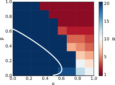
Figure 19: Dynamical state diagram of stochastic uptake of spherical particles using the phenomenological description of free membrane effects showing the maximum occupation probability of a trajectory of $N=10^{6}$ time steps. The white line corresponds to the state boundary of the deterministic model, cf. Fig. 13(c).

VII Conclusion

Here we have studied the uptake dynamics of nanometer-sized particles such as viruses at cell membranes mediated by ligand-receptor binding. The focus was on a simple but complete deterministic model, amenable to analytical insight, complemented by stochastic simulations.

By considering the adhesion, the bending and the tension energies of the cell membrane, including the contributions of the free, i.e. non-adhered membrane parts and calculating minimal energy membrane shapes numerically, we found that in the parameter regime which is typically relevant for biological systems, the free membrane contributes up to $20\%$ to the total energy during uptake. It thus cannot be neglected a priori. We hence incorporated the free membrane effects within a simple dynamical model for uptake by either a line tension or by an effective phenomenological description. This allowed us to study the deterministic uptake dynamics for spherical, cylindrical and spherocylindrical particles (both oriented either perpendicular or parallel to the membrane).

Similar to Huang et al. (2013); Dasgupta et al. (2014), where the uptake of spherocylindrical particles was studied, we find that the aspect ratio of cylindrical particles dictates the uptake pathway. While short cylinders are taken up fastest in normal mode, long cylinders are taken up fastest in parallel mode. For long cylinders at large reduced membrane tension one could speculate that they are taken up initially in parallel mode but might reorient driven by fluctuations to the perpendicular position in order to complete the uptake process Huang et al. (2013). Calculating the uptake times, spherical particles were found to be always taken up slower than cylinders. For spherocylindrical particles we found that they are always taken up fastest in parallel mode at equal volume and aspect ratio. When comparing them to spheres we found that while normal spherocylinders are taken up slower, for parallel spherocylinder the result depends on aspect ratio at equal volume. Our results regarding cylinders might change if one would include detailed models for adhesion and membrane shapes at the bottom and top faces. Here these effects are neglected to keep the model transparent.

For spherical particles, the free membrane effects influence the dynamics. In accordance with earlier work Deserno and Gelbart (2002); Deserno (2004); Vácha et al. (2011); Yi et al. (2011); Dasgupta et al. (2014), we could identify in the analytical model three scenarios for both the line tension and the phenomenological description of the free membrane: full uptake, partial uptake and no uptake, dictated by membrane elasticity, adhesion energy and the free membrane. There are, however, differences: the line tension induces an energy barrier (when considering the total energy) for small uptake angles for all parameters, hence uptake is only possible if assisted by fluctuations. In contrast, for the phenomenological description, the existence of this barrier depends on the parameters $\alpha$ and $\beta$. This is similar to the earlier work by Deserno and Gelbart Deserno and Gelbart (2002), where the shape of the free membrane shape is represented by a torus, that prevents uptake depending on particle size and the elasticity of the membrane. Considering the uptake speed, both the line tension and the phenomenological description speed up the process when passing over the equator. Overall we conclude that a line tension is not the best approach to describe the effects of the free membrane in the intermediate regime between tense and loose membranes. The phenomenological approach suggested here is clearly a better approximation. We presented a complete analysis of this case, focusing on steady states and dynamical state diagrams as a function of a reduced membrane tension ($\alpha$) and a reduced line tension ($\beta$). The occurrence of parameter regions of partial/no uptake could be traced back to new steady states emerging via saddle-node bifurcations.

Finally, we included stochasticity into the model as receptor-ligand binding is a discrete process in a small system such that fluctuations are expected to be important. This was achieved by mapping the deterministic models onto one-step master equations. In a first step, we used these to simulate and calculate uptake times. We could show that the effect of spheres profiting from noise and getting taken up faster than parallel cylinders, as described recently Frey et al. (2019), survives when free membrane effects are included. In a second step, we calculated stochastic state diagrams and again found surprisingly good agreement with the deterministic results. In both cases, it became clear that stochasticity enlarges the parameter region in which uptake is possible. Thus, fluctuations are expected to help the system to transverse barriers, corresponding to no uptake or partial uptake states, which could not be overcome in a deterministic model. In the future, our model could be extended by more detailed assumptions regarding the way the membrane moves forward and backward at the contact line. Such a description then could also describe the effect of temperature, which is not treated here, and of active membrane fluctuations, which would break detailed balance again.

Our uptake times are a lower bound to experimentally measured uptake times because we only consider the dissipative forces resulting from membrane microviscosity. Other mechanisms that might be rate-limiting include receptor diffusion within the plasma membrane, yielding uptake times in the few seconds range Gao et al. (2005), the assembly of clathrin lattices, with typical uptake times of the order of 60 seconds Kaksonen and Roux (2018), dissection of the cytoskeleton beneath the plasma membrane Stolp and Fackler (2011), and scission, with a timescale of minutes Shlomovitz et al. (2011). However, there is an increasing amount of experimental results showing that uptake times can indeed occur on the timescale of tens of milliseconds, including 250 ms for human enterovirus 71 Pan et al. (2017), around $80\,\mathrm{ms}$ for gold nanoparticles ($20\,\mathrm{nm}$) Ding et al. (2015), below $40\,\mathrm{ms}$ for the uptake of micrometer-sized latex beads by GUVs Dietrich et al. (1997) and even below 20 ms for silicon nanoparticles of ($4\,\mathrm{nm}$) diameter Wang et al. (2019). More importantly, however, is that our theory predicts very interesting effects regarding relative uptake times for different shapes. Our predictions in regard to the relative sequence of uptake and the phase diagrams do not depend on the absolute scale of the uptake time. They would only change if the dissipative uptake dynamics were not dominated by one single local time scale, for example if the advancement of the adhesion front was strongly limited by receptor diffusion Gao et al. (2005); Boulbitch et al. (2001). Finally our work suggests that both during biological evolution and for particle design in materials science, stochasticity might play an important role for optimal performance, which here is identified with fast uptake.

Appendix A Details on solving the shape equations

To numerically solve the boundary value problem given by Eq. (4), we rewrite it as a system of four first order ordinary differential equations. Three boundary conditions in Eq. (5) are given for $s\rightarrow\infty$. We hence use the asymptotic solution to shift the boundary conditions for the numerical problem to a finite arc length $s_{\mathrm{max}}$. For weak membrane deformations ($\psi\ll 1$) the linearized shape equations are solved by Foret (2014)

$$r(s)=s\,,\;\;\;\psi(s)=\beta K_{1}(s/\lambda)\,,\;\;\;z(s)=\beta\lambda K_{0}(s/\lambda)\,,$$ (50)

where $\beta=\theta/K_{1}(R/\lambda\sin\theta)$ is a parameter and $K_{n}$ are the modified Bessel functions of the second kind. Then the numerical boundary conditions using matched asymptotics read

$$r(0) =R\sin(\theta),$$

$$\psi(0) =\theta,$$

$$\psi(s_{\mathrm{max}}) =\beta{K_{1}(s_{\mathrm{max}}/\lambda)},$$

$$\dot{\psi}(s_{\mathrm{max}}) =-\frac{\beta}{2\lambda}\left(K_{0}(s_{\mathrm{max}}/\lambda)+K_{2}(s_{\mathrm{max}}/\lambda)\right),$$

$$z(s_{\mathrm{max}}) =\beta\lambda K_{0}(s_{\mathrm{max}}/\lambda).$$ (51)

The matching point $s_{\mathrm{max}}$ is then varied such that the computed solution fulfills $\psi(s_{\mathrm{max}})\ll 1$ and matching the numerical and asymptotic solution.

For comparison we also give the approximate asymptotic analytical solution for the energy of the free membrane as calculated in Foret (2014): in the limit of a tense membrane ($R\gg\lambda$) one has

$$\frac{E_{\mathrm{Foret}}^{\mathrm{tense}}}{\kappa}=4\pi\bigg{\{}\frac{4R}{\lambda}\sqrt{x(1-x)}(1-\sqrt{1-x})$$

$$-x-2\ln\left(\frac{1+\sqrt{1-x}}{2}\right)-2(1-\sqrt{1-x})^{2}\bigg{\}},$$ (52)

and for a loose membrane ($R\ll\lambda$)

$$\frac{E_{\mathrm{Foret}}^{\mathrm{loose}}}{\kappa}=4\pi\bigg{(}\frac{2R}{\lambda}x(1-x)\bigg{)}^{2}\times$$

$$\times\bigg{\{}-\gamma+\frac{x}{2(1-x)}-\ln\bigg{(}\frac{R}{\lambda}\sqrt{x(1-x)}(1-x)\bigg{)}\bigg{\}},$$ (53)

where $x=(1-\cos\theta)/2$ and the Euler constant $\gamma\approx 0.577$.

Appendix B Shape equations and energy of the free membrane for cylindrical particles with parallel orientation

For the parallel spherical particle the energy of the free membrane compared to the flat case can be written as

$$\frac{E_{\mathrm{free}}^{\mathrm{tot}}}{\kappa}=\int_{0}^{\infty}\left(\frac{\dot{\psi}^{2}}{2}+\frac{1-\cos\psi}{\lambda^{2}}\right)\,L\,\mathrm{d}s\,.$$ (54)

where we use a similar parametrisation and the same geometric relations as for the sphere

$$\dot{r}-\cos\psi =0,$$

$$\dot{z}+\sin\psi =0\,.$$ (55)

We construct a Lagrangian

$$\mathcal{L}=\dot{\psi}^{2}\frac{L}{2}+\frac{L}{\lambda^{2}}(1-\cos\psi)\,,$$ (56)

and find the Euler-Lagrange equations to equal

$$L\ddot{\psi}-\frac{L}{\lambda^{2}}\sin\psi=0$$

From Eq. (56) we construct a Hamiltonian by

$$\mathcal{H}=\dot{r}\partial_{\dot{r}}\mathcal{L}+\dot{\psi}\partial_{\dot{\psi}}\mathcal{L}-\mathcal{L}=\dot{\psi}^{2}\frac{L}{2}-\frac{L}{\lambda^{2}}(1-\cos\psi)\,.$$ (58)

Since $\mathcal{L}$ does not depend on $s$, $\mathcal{H}$ is conserved. Since the membrane is asymptotically flat $\mathcal{H}(s\rightarrow\infty)=0$ and thus $\mathcal{H}=0$ Foret (2018). Then,

$$\dot{\psi}=\pm\sqrt{\frac{2}{\lambda^{2}}(1-\cos\psi)}\,.$$ (59)

Using Eq. (59) in Eq. (54) we find

$$\frac{E_{\mathrm{free}}^{\mathrm{tot}}}{\kappa} =2\int_{0}^{\infty}\left(\frac{2}{\lambda^{2}}(1-\cos\psi)\right)\,L\,\mathrm{d}s\,,$$

$$=2L\sqrt{\frac{2}{\lambda^{2}}}\int_{0}^{\theta}\,\sqrt{(1-\cos\psi)}\mathrm{d}\psi\,,$$

$$=\frac{8L}{\lambda}\left(1-\cos\frac{\theta}{2}\right)\,,$$ (60)

where the factor 2 correspond to the left and right side of the membrane relative to the cylindrical particle. The same calculation and result can be found in Mkrtchyan et al. (2010).

References

- Auth et al. (2018) T. Auth, S. Dasgupta, and G. Gompper, in Physics of Biological Membranes (Springer, 2018) pp. 471–498.
- Zhang et al. (2015) S. Zhang, H. Gao, and G. Bao, ACS Nano 9, 8655 (2015).
- Alberts et al. (2017) B. Alberts, D. Bray, J. Watson, J. H. Lewis, and M. Raff, Molecular biology of the cell (Garland Science, 2017).
- Kumberger et al. (2016) P. Kumberger, F. Frey, U. S. Schwarz, and F. Graw, FEBS letters 590, 1972 (2016).
- Panyam and Labhasetwar (2003) J. Panyam and V. Labhasetwar, Adv. Drug Deliv. Rev. 55, 329 (2003).
- von Moos et al. (2012) N. von Moos, P. Burkhardt-Holm, and A. Köhler, Environ. Sci. Technol. 46, 11327 (2012).
- Gao et al. (2005) H. Gao, W. Shi, and L. B. Freund, Proc. Natl. Acad. Sci. (U.S.A.) 102, 9469 (2005).
- Barton et al. (2001) E. S. Barton, J. C. Forrest, J. L. Connolly, J. D. Chappell, Y. Liu, F. J. Schnell, A. Nusrat, C. A. Parkos, and T. S. Dermody, Cell 104, 441 (2001).
- Feldmann et al. (2003) H. Feldmann, S. Jones, H.-D. Klenk, and H.-J. Schnittler, Nat. Rev. Immunol. 3, 677 (2003).
- Matsumoto (1963) S. Matsumoto, J. Cell Biol. 19, 565 (1963).
- Lipowsky and Döbereiner (1998) R. Lipowsky and H.-G. Döbereiner, Europhys. Lett. 43, 219 (1998).
- Deserno (2004) M. Deserno, Phys. Rev. E 69, 031903 (2004).
- Agudo-Canalejo and Lipowsky (2015) J. Agudo-Canalejo and R. Lipowsky, ACS Nano 9, 3704 (2015).
- Decuzzi and Ferrari (2007) P. Decuzzi and M. Ferrari, Biomaterials 28, 2915 (2007).
- Yi et al. (2011) X. Yi, X. Shi, and H. Gao, Phys. Rev. Lett. 107, 098101 (2011).
- Zeng et al. (2017) C. Zeng, M. Hernando-Pérez, B. Dragnea, X. Ma, P. Van Der Schoot, and R. Zandi, Phys. Rev. Lett. 119, 038102 (2017).
- Sun and Wirtz (2006) S. X. Sun and D. Wirtz, Biophys. J. 90, L10 (2006).
- Yi and Gao (2017) X. Yi and H. Gao, Nanoscale 9, 454 (2017).
- Vácha et al. (2011) R. Vácha, F. J. Martinez-Veracoechea, and D. Frenkel, Nano Lett. 11, 5391 (2011).
- Huang et al. (2013) C. Huang, Y. Zhang, H. Yuan, H. Gao, and S. Zhang, Nano Lett. 13, 4546 (2013).
- Dasgupta et al. (2014) S. Dasgupta, T. Auth, and G. Gompper, Nano Lett. 14, 687 (2014).
- Bahrami et al. (2014) A. H. Bahrami, M. Raatz, J. Agudo-Canalejo, R. Michel, E. M. Curtis, C. K. Hall, M. Gradzielski, R. Lipowsky, and T. R. Weikl, Adv. Coll. Interf. Sci. 208, 214 (2014).
- Deng et al. (2019) H. Deng, P. Dutta, and J. Liu, Soft matter (2019).
- McDargh et al. (2016) Z. A. McDargh, P. Vázquez-Montejo, J. Guven, and M. Deserno, Biophys. J. 111, 2470 (2016).
- Frey et al. (2019) F. Frey, F. Ziebert, and U. S. Schwarz, Phys. Rev. Lett. 122, 088102 (2019).
- Foret (2014) L. Foret, Eur. Phys. J. E 37, 42 (2014).
- Helfrich (1973) W. Helfrich, Z. Naturforsch. C 28, 693 (1973).
- Kumar and Sain (2016) G. Kumar and A. Sain, Phys. Rev. E 94, 062404 (2016).
- Lipowsky (1992) R. Lipowsky, J. Phys. II (Paris) 2, 1825 (1992).
- Foret (2018) L. Foret, in Physics of Biological Membranes (Springer, 2018) pp. 385–419.
- Seifert et al. (1991) U. Seifert, K. Berndl, and R. Lipowsky, Phys. Rev. A 44, 1182 (1991).
- Jülicher and Seifert (1994) F. Jülicher and U. Seifert, Phys. Rev. E 49, 4728 (1994).
- (33) Using the function: ‘scipy integrate solve bvp’ from Jones et al. (01) .
- Mkrtchyan et al. (2010) S. Mkrtchyan, C. Ing, and J. Z. Chen, Phys. Rev. E 81, 011904 (2010).
- Reister-Gottfried et al. (2008) E. Reister-Gottfried, K. Sengupta, B. Lorz, E. Sackmann, U. Seifert, and A.-S. Smith, Phys. Rev. Lett. 101, 208103 (2008).
- Weikl et al. (2009) T. R. Weikl, M. Asfaw, H. Krobath, B. Różycki, and R. Lipowsky, Soft Matter 5, 3213 (2009).
- Turlier et al. (2016) H. Turlier, D. A. Fedosov, B. Audoly, T. Auth, N. S. Gov, C. Sykes, J.-F. Joanny, G. Gompper, and T. Betz, Nat. Phys. 12, 513 (2016).
- Cremer et al. (2012) J. Cremer, A. Melbinger, and E. Frey, Sci. Rep. 2, 281 (2012).
- Melbinger et al. (2010) A. Melbinger, J. Cremer, and E. Frey, Phys. Rev. Lett. 105, 178101 (2010).
- Van Kampen (1992) N. G. Van Kampen, Stochastic processes in physics and chemistry, Vol. 1 (Elsevier, 1992).
- Gillespie (1977) D. T. Gillespie, J. Phys. Chem. 81, 2340 (1977).
- Osaki et al. (2004) F. Osaki, T. Kanamori, S. Sando, T. Sera, and Y. Aoyama, J. Am. Chem. Soc. 126, 6520 (2004).
- Zhang et al. (2009) S. Zhang, J. Li, G. Lykotrafitis, G. Bao, and S. Suresh, Adv. Mater. 21, 419 (2009).
- Deserno and Gelbart (2002) M. Deserno and W. M. Gelbart, J. Phys. Chem. B 106, 5543 (2002).
- Kaksonen and Roux (2018) M. Kaksonen and A. Roux, Nat. Rev. Mol. Cell Bio. 19, 313 (2018).
- Stolp and Fackler (2011) B. Stolp and O. T. Fackler, Viruses 3, 293 (2011).
- Shlomovitz et al. (2011) R. Shlomovitz, N. Gov, and A. Roux, New J. Phys. 13, 065008 (2011).
- Pan et al. (2017) Y. Pan, F. Zhang, L. Zhang, S. Liu, M. Cai, Y. Shan, X. Wang, H. Wang, and H. Wang, Adv. Sci 4, 1600489 (2017).
- Ding et al. (2015) B. Ding, Y. Tian, Y. Pan, Y. Shan, M. Cai, H. Xu, Y. Sun, and H. Wang, Nanoscale 7, 7545 (2015).
- Dietrich et al. (1997) C. Dietrich, M. Angelova, and B. Pouligny, J. Phys. II 7, 1651 (1997).
- Wang et al. (2019) R. Wang, X. Yang, D. Leng, Q. Zhang, D. Lu, S. Zhou, Y. Yang, G. Yang, and Y. Shan, Anal. Methods (2019).
- Boulbitch et al. (2001) A. Boulbitch, Z. Guttenberg, and E. Sackmann, Biophys. J. 81, 2743 (2001).
- Jones et al. (01 ) E. Jones, T. Oliphant, P. Peterson, et al., “SciPy: Open source scientific tools for Python,” (2001–).