Twenty Hopf-like bifurcations in piecewise-smooth dynamical systems.

Abstract

For many physical systems the transition from a stationary solution to sustained small amplitude oscillations corresponds to a Hopf bifurcation. For systems involving impacts, thresholds, switches, or other abrupt events, however, this transition can be achieved in fundamentally different ways. This paper reviews 20 such ‘Hopf-like’ bifurcations for two-dimensional ODE systems with state-dependent switching rules. The bifurcations include boundary equilibrium bifurcations, the collision or change of stability of equilibria or folds on switching manifolds, and limit cycle creation via hysteresis or time delay. In each case a stationary solution changes stability and possibly form, and emits one limit cycle. Each bifurcation is analysed quantitatively in a general setting: we identify quantities that govern the onset, criticality, and genericity of the bifurcation, and determine scaling laws for the period and amplitude of the resulting limit cycle. Complete derivations based on asymptotic expansions of Poincaré maps are provided. Many of these are new, done previously only for piecewise-linear systems. The bifurcations are collated and compared so that dynamical observations can be matched to geometric mechanisms responsible for the creation of a limit cycle. The results are illustrated with impact oscillators, relay control, automated balancing control, predator-prey systems, ocean circulation, and the McKean and Wilson-Cowan neuron models.

 

1 Introduction

Sustained oscillations are central to many dynamical systems. Ocean and atmospheric oscillations drive global weather patterns, and seasonal variations direct annual cycles such as the Arctic sea ice extent Di13 ; KaEn13 . An understanding of these oscillations may lead to better predictions regarding anthropogenic climate change. Biological systems involve oscillations on diverse scales, from circadian rhythms and day/night cycles to intra-cellular processes and neural firing Fo17 ; KeSn98 ; Wi01 . Detailed knowledge of such oscillations is crucial to preventing and treating improper functioning such as cardiac arrhythmia. Also mechanical systems oscillate both by design and as unwanted vibrations Di10 ; DuSr12 .

Mathematically an oscillation is a loop in phase space: the abstract space representing all possible states of a system. The loop is traced by the state of the system as time evolves. For systems of ODEs (ordinary differential equations) the loop is a periodic orbit and called a limit cycle if it is isolated from other periodic orbits.

For many systems limit cycles only exist over some range of parameter values. At the endpoints of the parameter range the limit cycle is created or destroyed in a bifurcation, the simplest of which is a Hopf bifurcation. At a Hopf bifurcation an equilibrium loses stability (more generally its stable and unstable manifolds change dimension) and a small amplitude limit cycle is created. The bifurcation occurs when a complex conjugate pair of eigenvalues associated with the equilibrium crosses the imaginary axis in the complex plane. Hopf bifurcations are important in fluid dynamics MaTu95 , laser physics NiHa90 , and ecology FuEl00 ; for further examples refer to the classic texts HaKa81 ; MaMc76 .

This paper concerns piecewise-smooth systems for which phase space contains one or more switching manifolds where a map is applied or the functional form of the equations of motion changes (as in Fig. 1.1). Piecewise-smooth ODEs form natural mathematical models of relay control systems BaVe01 ; Jo03 ; ZhMo03 , mechanical systems with impacts AwLa03 ; Br99 ; WiDe00 , and phenomena in other areas including climate science Wi13 , neuroscience KeHo81 , and ecology DeGr07 .

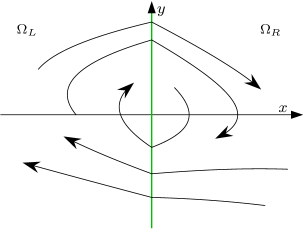
Figure 1.1: A sketch of the phase space of a two-dimensional piecewise-smooth ODE system with switching manifold, $x=0$. The switching manifold divides phase space into two regions, $\Omega_{L}$ and $\Omega_{R}$, where the ODEs are smooth. Parts of typical orbits are shown.

#	description	bifurcation onset	non-degeneracy coefficient, $\alpha$	amplitude exponent, $a$	period exponent, $b$	key ,reference(s),
-	Hopf	$\omega=0$	(2.5)	$1/2$	$0$	AnWi30 ; Ho42 ; Po92
$1$	focus/focus BEB	BEB	$\frac{\lambda_{L}}{\omega_{L}}+\frac{\lambda_{R}}{\omega_{R}}$	$1$	$0$	FrPo97 ; SiMe07
$2$	focus/node BEB	BEB	-	$1$	$0$	FrPo98
$3$	generic BEB	BEB	-	$1$	$0$	Fi88 ; KuRi03
$4$	degenerate BEB	BEB	$\frac{\lambda_{L}}{\omega_{L}}+\frac{\lambda_{R}}{\omega_{R}}$	$1$	$0$	Si18f
$5$	slipping foci	collision	$\frac{\lambda_{L}}{\omega_{L}}+\frac{\lambda_{R}}{\omega_{R}}$	$1$	$0$	CaLl17
$6$	slipping focus/fold	collision	$\lambda_{L}$	$1$	$0$	CaLl17
$7$	slipping folds	collision	$\sigma_{{\rm fold},L}-\sigma_{{\rm fold},R}$	$1/2$	$1/2$	CaLl17 ; KuRi03
$8$	fixed foci	$\frac{\lambda_{L}}{\omega_{L}}+\frac{\lambda_{R}}{\omega_{R}}=0$	$\chi_{{\rm focus},L}-\chi_{{\rm focus},R}$	$1$	$0$	CoGa01 ; ZoKu06
$9$	fixed focus/fold	$\lambda_{L}=0$	$\chi_{{\rm focus},L}-\frac{\sigma_{{\rm fold},R}}{3}$	$1$	$0$	CoGa01
$10$	fixed folds	$\sigma_{{\rm fold},L}=\sigma_{{\rm fold},R}$	$\chi_{{\rm fold},L}-\chi_{{\rm fold},R}$	$1/2$	$1/2$	LiHu14
$11$	impacting admissible focus	BEB	(9.9)	$1$	$0$	DiNo08
$12$	impacting virtual focus	BEB	(9.9)	$1$	$0$	DiNo08
$13$	impacting virtual node	BEB	-	$1$	$0$	DiNo08
$14$	impulsive	(9.20)	(9.25)	$1$	$0$	Ak05
$15$	hysteretic pseudo-eq.	hysteresis	(10.7)	$1$	$1$	MaHa17
$16$	time delayed pseudo-eq.	time delay	(10.7)	$1$	$1$	LiYu08
$17$	hysteretic two-fold	hysteresis	$\sigma_{{\rm fold},L}-\sigma_{{\rm fold},R}$	$1/3$	$1/3$	Ma17
$18$	time delayed two-fold	time delay	$\sigma_{{\rm fold},L}-\sigma_{{\rm fold},R}$	$1/2$	$1/2$	Ko17 ; LiYu13
$19$	intersecting sw. manifolds	(11.3)	(11.7)	$1$	$1$	HaEr15
$20$	square-root singularity	BEB	-	$1$	$0$	NiCa16

Table 1.1: Attributes of Hopf bifurcations and $20$ Hopf-like bifurcations (HLBs). The HLBs are numbered 1–20, as indicated in the first column; the second column gives a brief description (BEB abbreviates boundary equilibrium bifurcation). The exponents $a$ and $b$ refer to the scaling laws (1.1) and for most HLBs the stability of the limit cycle (i.e. the criticality of the bifurcation) is determined by the sign of $\alpha$. Full details including formulas for $\alpha$ and additional references are provided in later sections. Note, $\alpha$ is not specified for four HLBs where criticality is governed a combination of algebraic constraints.

Piecewise-smooth systems admit several types of stationary solutions (where the state of the system is constant in time). These include regular equilibria (a zero of a smooth component of the vector field) and certain points on switching manifolds. Interactions between stationary solutions and switching manifolds induce a wide variety of bifurcations that are unique to piecewise-smooth systems DiBu08 . This paper concerns such bifurcations that are ‘Hopf-like’ in the sense that an isolated stationary solution changes stability and possibly form and emits one limit cycle locally OlAn04 . While there have been numerous studies of Hopf-like bifurcations (HLBs), many focus on one particular scenario, consider only piecewise-linear systems, or provide only qualitative results. The purpose of this paper is provide general quantitative results and compare different HLBs. This extends the summary presented in Si18c ; below we provide formal statements for each HLB in a general setting.

So that the geometric mechanisms underpinning the HLBs can be realised with minimal complexity, only two-dimensional systems are treated. In more than two dimensions HLBs can occur in an essentially two-dimensional fashion KuHo13 ; SiKo09 , but other dynamics (including chaos) may be involved Gl18 ; Si16c ; Si18d . HLBs have been described in three-dimensional systems CaFe11 ; CaFe12 ; CaFr05b ; FrPo05 ; FrPo07 ; HuYa16 and some limited forms of dimension reduction have been achieved KoGl11 ; Ku08 ; KuHo13 ; PrTe16 ; WeKu12 , but in general higher dimensions cannot be accommodated via a centre manifold analysis (the standard approach used for smooth systems Ku04 ; Me07 ) because a centre manifold simply may not exist. Much of the bifurcation theory of piecewise-smooth systems is dimension specific. In $n$ dimensions bifurcations can be inextricably $n$-dimensional GlJe15 .

The HLBs are labelled $1$–$20$ and summarised by Table 1.1. The first two columns provide the number and a brief description. The next two columns indicate the cause or onset of the bifurcation and give a formula for the non-degeneracy coefficient $\alpha$. In most cases a stable limit cycle is created if $\alpha<0$ and unstable limit cycle is created if $\alpha>0$. For example, a (classical) Hopf bifurcation occurs when the imaginary part $\omega$ of the associated eigenvalues is zero, and $\alpha$ is a combination of quadratic and cubic terms in a Taylor expansion of the ODEs, see (2.5). Several HLBs are boundary equilibrium bifurcations (BEBs) that occur when a regular equilibrium collides with a switching manifold.

The next two columns provide scaling laws for the amplitude of the limit cycle (as measured by its diameter in phase space) and its period. If a HLB occurs at $\mu=0$, where $\mu\in\mathbb{R}$ is a parameter, then the limit cycle exists for small $\mu<0$ or small $\mu>0$ and satisfies

$$\begin{split}\text{amplitude}&\sim k_{1}|\mu|^{a},\\ \text{period}&\sim k_{2}|\mu|^{b}.\end{split}$$ (1.1)

The exponents $a>0$ and $b\geq 0$ are determined by the type of HLB; the coefficients $k_{1}>0$ and $k_{2}>0$ are system specific. For Hopf bifurcations, $a=\frac{1}{2}$ (square-root growth) and $b=0$ (the period limits to $\frac{2\pi}{\omega}$ at the bifurcation). For a physical system, $a$ and $b$ could be estimated experimentally in which case the results here could assist model selection in that models involving HLBs with incorrect values of $a$ and $b$ would be discarded.

The HLBs described here are local bifurcations. For piecewise-smooth systems, limit cycles can be created in global bifurcations such as ‘canard super-explosions’ where an equilibrium transitions instantaneously to a large amplitude limit cycle DeFr13 ; RoGl14 ; RoCo12 ; WaWi16 , For piecewise-linear systems, a limit cycle may be created at infinity LlPo99 , and if there are two switching manifolds a limit cycle intersecting both manifolds may appear suddenly LlOr13 ; LlPo15 ; PoRo15 ; ToGe03 .

Other bifurcations not considered here include those at which two equilibria and a local limit cycle emanate from a single point on a switching manifold. Such bifurcations combine the characteristic features of saddle-node and Hopf bifurcations and arise in continuous systems SiMe12 , discontinuous systems KuRi03 ; PoRo18 , and impacting systems DiNo08 . The bifurcation of an equilibrium into two limit cycles has been described in switched control systems SiKu12b , impacting systems MoBu14 , and abstract piecewise-linear systems ArLl14 ; DiEl14 . Remarkably, the bifurcation of an equilibrium into three limit cycles is possible for two-dimensional piecewise-linear discontinuous systems, see BrMe13 ; FrPo14 ; HuYa12b ; Li14 ; LlNo15 . For codimension-two HLBs refer to DeDe11 ; DiPa08 ; GiPl01 ; GuSe11 ; SiMe08 and for non-autonomous perturbations (e.g. periodic forcing) see FePo16 .

The remainder of this paper is organised as follows. We begin in §2 by reviewing Hopf bifurcations and stating the Hopf bifurcation theorem in a way that is later mimicked, as much as possible, with the HLBs. In §3 we review geometric aspects of piecewise-smooth systems (particularly Filippov systems) such as folds, pseudo-equilibria, and sliding motion. Section 4 provides some technical results to support the proofs of the main theorems. Each proof is based on the construction and analysis of a locally valid Poincaré map. An isolated fixed point of a Poincaré map corresponds to limit cycle. Most of the Poincaré maps are constructed by combining two maps, one for the system on each side of a switching manifold. These two maps are return maps, capturing the effect of evolution from, and back to, a switching manifold. In §4 we provide asymptotic expansions for return maps about an invisible fold, a boundary focus, and a regular focus in an affine system (Lemmas 4.4–4.6). We also review our key analytical tool: the implicit function theorem (IFT), and discuss the degree of smoothness of orbits and Poincaré maps.

The HLBs are examined in Sections 5–11 in order. For each HLB we provide a theorem, an example, and a proof (given in an appendix). Most theorems have the following features. There exists an isolated stationary solution for all values of $\mu$ in a neighbourhood of $0$. There is a transversality condition $\beta\neq 0$ (to ensure that $\mu$ unfolds the bifurcation in a generic fashion). Where appropriate $\beta$ is defined so that $\beta>0$ (chosen without loss of generality in view of the substitution $\mu\mapsto-\mu$) implies the stationary solution is stable for $\mu<0$ and unstable for $\mu>0$. When $\mu=0$ the stationary solution is stable if $\alpha<0$ and unstable if $\alpha>0$. If $\alpha<0$ then the bifurcation is supercritical (a stable limit cycle exists for small $\mu>0$), while if $\alpha>0$ then the bifurcation is subcritical (an unstable limit cycle exists for small $\mu<0$). Then §12 provides concluding remarks.

The theorems are proved in appendices by identifying a unique fixed point of a Poincaré map $P$ via the IFT (an alternative is to use the intermediate value theorem for monotone functions). Many of these involve a spatial scaling to ‘blow up’ the dynamics about the origin, or a brute-force evaluation of terms (using Lemmas 4.4 and 4.5), but several have unique technical complexities. For instance, HLB 4 requires a careful analysis of nonlinear functions, HLB 17 uses a non-constructive derivation, and HLB 20 requires a multiple time-scales analysis. The IFT is usually applied to a displacement function $D(r;\mu)$ whose zeros correspond to fixed points of $P(r;\mu)$. For example, for HLBs $8$, $9$, $14$, and $19$ we use $D(r;\mu)=\frac{1}{r}\mathopen{}\mathclose{{}\left(P(r;\mu)-r}\right)$ so that the $r=0$ fixed point (corresponding to a stationary solution at the origin) is removed. Typically $D$ is only defined for, say, $r>0$, so $D$ must be smoothly extended to a neighbourhood of $(r;\mu)=(0;0)$ before the IFT is applied.

2 Hopf bifurcations

The mathematicians most closely affiliated with Hopf bifurcations are Poincaré, Andronov, and Hopf. Poincaré studied Hopf bifurcations in the late $19^{\rm th}$ century Po92 , Andronov and coworkers later proved the Hopf bifurcation theorem for two-dimensional systems of ODEs AnWi30 , and this was extended by Hopf to systems of arbitrary dimension in Ho42 . Hopf bifurcations generalise to other equations, such as partial differential equations HaKa81 ; MaMc76 ; Se94 , delay differential equations Er09 ; HaLu93 , and stochastic differential equations ArSr96 .

Here we state the Hopf bifurcation theorem, following Gl99 , for a two-dimensional system,

$$\begin{bmatrix}\dot{x}\\ \dot{y}\end{bmatrix}=F(x,y;\mu)=\begin{bmatrix}f(x,y;\mu)\\ g(x,y;\mu)\end{bmatrix},$$ (2.1)

where $\mu\in\mathbb{R}$ is a parameter. Throughout this paper dots represents differentiation with respect to time, $t$. We first make two assumptions that allow us to state the theorem concisely. For a general system these assumptions can be imposed by performing an appropriate change of variables.

We first assume that the origin is an equilibrium for all values of $\mu$ in a neighbourhood of $0$ (this simplifies the formula for $\beta$ given below). That is,

$$f(0,0;\mu)=g(0,0;\mu)=0,$$ (2.2)

for small $\mu\in\mathbb{R}$. Second we assume

$${\rm D}F(0,0;0)=\begin{bmatrix}0&-\omega\\ \omega&0\end{bmatrix},$$ (2.3)

for some $\omega\neq 0$. That is, when $\mu=0$ the eigenvalues associated with the origin are $\pm{\rm i}\omega$, and the Jacobian matrix is in real Jordan form.

In order for $\mu$ to unfold the Hopf bifurcation in a generic fashion, the real part of the eigenvalues associated with the equilibrium must change linearly, to leading order, with respect to $\mu$. A simple calculation reveals that the real part of the eigenvalues is $\frac{\beta\mu}{2}+O\mathopen{}\mathclose{{}\left(\mu^{2}}\right)$, where

$$\beta=\mathopen{}\mathclose{{}\left(\frac{\partial^{2}f}{\partial\mu\partial x}+\frac{\partial^{2}g}{\partial\mu\partial y}}\right)\bigg{|}_{x=y=\mu=0}.$$ (2.4)

Consequently, $\beta\neq 0$ is the transversality condition for the Hopf bifurcation theorem.

We also require the quadratic and cubic terms in the Taylor expansion of $F(x,y;0)$ (centred about the origin) to be such that a limit cycle is created in a non-degenerate fashion. To this end, we define

$$\alpha =\mathopen{}\mathclose{{}\left(\frac{\partial^{3}f}{\partial x^{3}}+\frac{\partial^{3}g}{\partial x^{2}\partial y}+\frac{\partial^{3}f}{\partial x\partial y^{2}}+\frac{\partial^{3}g}{\partial y^{3}}}\right)\bigg{|}_{x=y=\mu=0}$$

$$\quad+\frac{1}{\omega}\bigg{[}\frac{\partial^{2}f}{\partial x\partial y}\mathopen{}\mathclose{{}\left(\frac{\partial^{2}f}{\partial x^{2}}+\frac{\partial^{2}f}{\partial y^{2}}}\right)-\frac{\partial^{2}f}{\partial x^{2}}\frac{\partial^{2}g}{\partial x^{2}}$$

$$\quad-\frac{\partial^{2}g}{\partial x\partial y}\mathopen{}\mathclose{{}\left(\frac{\partial^{2}g}{\partial x^{2}}+\frac{\partial^{2}g}{\partial y^{2}}}\right)+\frac{\partial^{2}f}{\partial y^{2}}\frac{\partial^{2}g}{\partial y^{2}}\bigg{]}\bigg{|}_{x=y=\mu=0}.$$ (2.5)

At the bifurcation (i.e. with $\mu=0$), nearby orbits converge to the origin as $t\to\infty$ if $\alpha<0$, and as $t\to-\infty$ if $\alpha>0$. For this reason, $\alpha\neq 0$ is the non-degeneracy condition for the Hopf bifurcation theorem.

Theorem 2.1 (Hopf bifurcation theorem).

Consider (2.1) where $F$ is $C^{3}$. Suppose (2.2) and (2.3) are satisfied and $\beta>0$. In a neighbourhood of $(x,y;\mu)=(0,0;0)$,

1. the origin is the unique equilibrium and is stable for $\mu<0$ and unstable for $\mu>0$,

2. if $\alpha<0$ [$\alpha>0$] there exists a unique stable [unstable] limit cycle for $\mu>0$ [$\mu<0$], and no limit cycle for $\mu<0$ [$\mu>0$].

The minimum and maximum $x$ and $y$-values of the limit cycle are asymptotically proportional to $\sqrt{|\mu|}$, and its period is $T=\frac{2\pi}{|\omega|}+O(\mu)$.

The Hopf bifurcation theorem can be proved by performing a sequence of near-identity transformations so that in polar coordinates, or with a single complex-valued variable, the ODEs take a simple form. The proof can then be completed by using the Poincaré-Bendixson theorem, as in Gl99 , or applying the implicit function theorem to a Poincaré map, as in HaKa81 ; MaMc76 .

Figure 2.1: An illustration of the Hopf bifurcation for the van der Pol oscillator (2.6) with $k_{2}=1$. The bifurcation diagram shows the equilibrium and the maximum and minimum $x$-values of the limit cycle. Stable solutions are coloured blue; unstable solutions are coloured red. These conventions are used in all subsequent bifurcation diagrams.

The Hopf bifurcation theorem can be illustrated with the van der Pol oscillator Va26 . Following Me07 , we consider

$$\begin{split}\frac{dv}{dt}&=i,\\ \frac{di}{dt}&=-v+k_{1}i-k_{2}i^{3},\end{split}$$ (2.6)

where $i(t)$ represents the non-dimensionalised current in a circuit with a capacitor, an inductor, and an additional element (vacuum tube or tunnel diode) with voltage drop $-k_{1}i+k_{2}i^{3}$, and $v(t)$ represents the non-dimensionalised voltage at a particular location in the circuit.

The origin, $(v,i)=(0,0)$, is an equilibrium of (2.6) and has purely imaginary eigenvalues when $k_{1}=0$. Indeed the Hopf bifurcation theorem, as stated above, can be applied directly using $(x,y;\mu)=(v,i;k_{1})$. The transversality coefficient is $\beta=1$ and the non-degeneracy coefficient is $\alpha=-6k_{2}$. Fig. 2.1 shows a bifurcation diagram and representative phase portraits using $k_{2}=1$. Here $\alpha<0$, thus a stable limit cycle exists for $k_{1}>0$ as shown. Notice the amplitude of the limit cycle is proportional to $\sqrt{k_{1}}$, to leading order.

3 Fundamentals of Filippov systems

Filippov systems are discontinuous, piecewise-smooth ODE systems with an additional rule defining evolution on switching manifolds, known as sliding motion. Here we review the basic principles of Filippov systems for two-dimensional systems with a single switching manifold. More general expositions can be found in CoDi12 ; DiBu08 ; Fi88 ; Je18b .

We consider ODE systems on $\mathbb{R}^{2}$ of the form

$$\begin{bmatrix}\dot{x}\\ \dot{y}\end{bmatrix}=\begin{cases}F_{L}(x,y),&x<0,\\ F_{R}(x,y),&x>0.\end{cases}$$ (3.1)

Here the switching manifold is $x=0$. For systems with a more general switching manifold, say $H(x,y)=0$, the idea is that one may perform a change of variables to put the system in the form (3.1). The change of variables may only be valid locally, but this is sufficient for the local bifurcation theory of this paper.

We let

$$\begin{split}\Omega_{L}&=\mathopen{}\mathclose{{}\left\{(x,y)\,\middle|\,x<0,y\in\mathbb{R}}\right\},\\ \Omega_{R}&=\mathopen{}\mathclose{{}\left\{(x,y)\,\middle|\,x>0,y\in\mathbb{R}}\right\},\end{split}$$ (3.2)

denote the left and right half-planes. We refer to $(\dot{x},\dot{y})=F_{L}(x,y)$ and $(\dot{x},\dot{y})=F_{R}(x,y)$ as the left and right half-systems of (3.1), respectively. Orbits of (3.1) are governed by the left half-system while in $\Omega_{L}$, and by the right half-system while in $\Omega_{R}$. Orbits may also slide on $x=0$, as defined below.

To ensure sliding motion is well-defined, we assume $F_{J}$ is $C^{1}$ on the closure of $\Omega_{J}$, for each $J\in\{L,R\}$. In mathematical models each $F_{J}$ is often well-defined (or extends analytically) beyond $\Omega_{J}$, in which case we can consider the dynamics of $(\dot{x},\dot{y})=F_{J}(x,y)$ outside $\Omega_{J}$ — such dynamics is termed virtual. Virtual dynamics is not exhibited by (3.1), but sometimes helps us understand the behaviour of (3.1). We use the term admissible to describe dynamics of $(\dot{x},\dot{y})=F_{J}(x,y)$ in $\Omega_{J}$.

Definition 3.1.

A regular equilibrium of (3.1) is a point $(x,y)$ for which $F_{L}(x,y)=(0,0)$ or $F_{R}(x,y)=(0,0)$.

If $F_{L}(x,y)=(0,0)$, then the equilibrium is admissible if $x<0$ and virtual if $x>0$ (and vice-versa if $F_{R}(x,y)=(0,0)$). As parameters are varied, an admissible equilibrium becomes virtual when it collides with $x=0$, where it is termed a boundary equilibrium. This is known as a boundary equilibrium bifurcation (BEB) DiBu08 . Many of the HLBs below are BEBs.

Next we distinguish different parts of the switching manifold, and to do this write

$$F_{J}(x,y)=\begin{bmatrix}f_{J}(x,y)\\ g_{J}(x,y)\end{bmatrix},$$ (3.3)

for each $J\in\{L,R\}$.

Definition 3.2.

A subset $\mathopen{}\mathclose{{}\left\{(0,y)\,\middle|\,y\in(a,b)}\right\}$ of $\Sigma$ is said to be

1. a crossing region if $f_{L}(0,y)f_{R}(0,y)>0$ for all $y\in(a,b)$,

2. an attracting sliding region if $f_{L}(0,y)>0$ and $f_{R}(0,y)<0$ for all $y\in(a,b)$,

3. and a repelling sliding region if $f_{L}(0,y)<0$ and $f_{R}(0,y)>0$ for all $y\in(a,b)$.

Orbits of (3.1) are directed into attracting sliding regions, away from repelling sliding regions, and through crossing regions (see already Fig. 3.1). At endpoints of these regions we have $f_{J}(0,y)=0$, for some $J\in\{L,R\}$. If $f_{J}(0,y)=0$ and $g_{J}(0,y)\neq 0$, then $F_{J}(0,y)$ is tangent to $x=0$. If also $\frac{\partial f_{J}}{\partial y}(0,y)\neq 0$, then the orbit of the associated half-system that passes through $(0,y)$ has a quadratic tangency with $x=0$ at this point. In this case the tangent point is called a fold, and said to be visible if the orbit is admissible and invisible if it is virtual:

Definition 3.3.

A point $(0,y)$ for which $f_{L}(0,y)=0$ [$f_{R}(0,y)=0$] is said to be

1. a visible fold if $\frac{\partial f_{L}}{\partial y}(0,y)g_{L}(0,y)<0$
   $\mathopen{}\mathclose{{}\left[\frac{\partial f_{R}}{\partial y}(0,y)g_{R}(0,y)>0}\right]$,

2. and an invisible fold if $\frac{\partial f_{L}}{\partial y}(0,y)g_{L}(0,y)>0$
   $\mathopen{}\mathclose{{}\left[\frac{\partial f_{R}}{\partial y}(0,y)g_{R}(0,y)<0}\right]$.

For example, the system

$$\begin{bmatrix}\dot{x}\\ \dot{y}\end{bmatrix}=\begin{cases}\begin{bmatrix}y\\ 1\end{bmatrix},&x<0,\\ \begin{bmatrix}-2(y-1)\\ -1\end{bmatrix},&x>0,\end{cases}$$ (3.4)

depicted in Fig. 3.1, has a visible fold at $(0,1)$ and an invisible fold at $(0,0)$.

Two-folds are points at which $f_{L}(0,y)=f_{R}(0,y)=0$, and are naturally classified as visible-visible, visible-invisible, invisible-invisible, or degenerate. For the two-dimensional system (3.1), two-folds are codimension-one phenomena and can correspond to the creation of a limit cycle (HLB 7). In three-dimensional systems, two-folds occur generically and may serve as a hub for important dynamics CoJe11 ; CrCa17 ; DiCo11 ; Te90 .

On sliding regions (both attracting and repelling) we can define orbits by introducing a one-dimensional vector field:

$$\dot{y}=g_{\rm slide}(y).$$ (3.5)

To motivate the definition of $g_{\rm slide}$ we first present the general notion of a Filippov solution.

Definition 3.4.

An absolutely continuous function $\phi_{t}:(a,b)\to\mathbb{R}^{2}$ is said to be a Filippov solution to (3.1) if it satisfies $\dot{\phi}_{t}\in\mathcal{F}(\phi_{t})$ for almost all $t\in(a,b)$, where $\mathcal{F}$ is the set-valued function

$$\mathcal{F}(x,y)=\begin{cases}\{F_{L}(x,y)\},&x<0,\\ \mathopen{}\mathclose{{}\left\{(1-s)F_{L}(0,y)+sF_{R}(0,y)\,\big{|}\,s\in[0,1]}\right\},&x=0,\\ \{F_{R}(x,y)\},&x>0.\end{cases}$$ (3.6)

The system (3.1) is a Filippov system if we equate orbits to Filippov solutions. Notice $\mathcal{F}(0,y)$ is defined as the convex hull of $F_{L}(0,y)$ and $F_{R}(0,y)$. For more general systems $\mathcal{F}$ is defined as the convex hull of all smooth components of the system associated with each point.

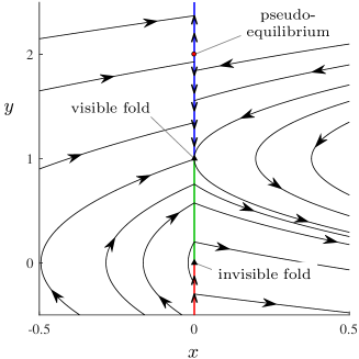
Figure 3.1: A phase portrait of the Filippov system (3.4). The switching manifold $x=0$ is a crossing region for $0<y<1$ (green), an attracting sliding region for $y>1$ (blue), and a repelling sliding region for $y<0$ (red). On the sliding regions arrows indicate the direction of sliding motion.

Now consider a Filippov solution $\phi_{t}$ that is constrained to a sliding region for some interval of time. In order to express the $y$-component of $\phi_{t}$ as a solution to (3.5), we use Definition 3.6 to construct $g_{\rm slide}$. The condition $\dot{\phi}_{t}\in\mathcal{F}(\phi_{t})$ implies that the $x$-component of $(1-s)F_{L}(0,y)+sF_{R}(0,y)=0$ is zero. Thus $s=\frac{f_{L}}{f_{L}-f_{R}}\big{|}_{x=0}$ and notice $s\in(0,1)$ because we are considering a sliding region. By then defining $g_{\rm slide}$ as the $y$-component of $(1-s)F_{L}(0,y)+sF_{R}(0,y)$:

$$g_{\rm slide}=\mathopen{}\mathclose{{}\left.\frac{f_{L}g_{R}-f_{R}g_{L}}{f_{L}-f_{R}}}\right|_{x=0}\,,$$ (3.7)

the $y$-component of $\phi_{t}$ is a solution to (3.5) as desired.

Definition 3.5.

A point $(0,y)$ is said to be a pseudo-equilibrium of (3.1) if $g_{\rm slide}(y)=0$.

The pseudo-equilibrium is admissible if $f_{L}(0,y)f_{R}(0,y)<0$ (i.e. it belongs to a sliding region) and virtual if $f_{L}(0,y)f_{R}(0,y)>0$. As an example, again consider (3.4). Here $g_{\rm slide}(y)=\frac{y-2}{3y-2}$, thus there is a unique pseudo-equilibrium at $(0,2)$. This pseudo-equilibrium is unstable because $\frac{dg_{\rm slide}}{dy}\big{|}_{y=2}>0$.

To summarise, orbits of the Filippov system (3.1) are piecewise: governed by the left half-system in $\Omega_{L}$, by the right half-system in $\Omega_{R}$, and by (3.5) with (3.7) on sliding regions. The forward orbit of a point can be non-unique. For instance, the forward orbit of a point on a repelling sliding region can immediately enter $\Omega_{L}$, immediately enter $\Omega_{R}$, or slide along $x=0$ for some time before entering $\Omega_{L}$ or $\Omega_{R}$.

4 Return maps and smoothness

To study limit cycles in systems of the form (3.1) we construct Poincaré maps by using the switching manifold $x=0$ as a Poincaré section. Each Poincaré map is a composition $P=P_{L}\circ P_{R}$, where $P_{R}$ is the return map on $x=0$ for orbits of the right half-system, and $P_{L}$ is the return map on $x=0$ for orbits of the left half-system, see Fig. 4.1. In this section we first clarify the smoothness of orbits and return maps, §4.1. We then derive three return maps on $x=0$ for evolution in $x>0$ for a smooth system

$$\begin{bmatrix}\dot{x}\\ \dot{y}\end{bmatrix}=F(x,y)=\begin{bmatrix}f(x,y)\\ g(x,y)\end{bmatrix}.$$ (4.1)

These maps are used below for $P_{R}$ and also $P_{L}$ through a change of variables such as $(x,y)\mapsto(-x,-y)$. For the first map the origin is a focus, §4.2; for the second map the origin is an invisible fold (treating (4.1) as the right half-system of (3.1)), §4.3. For these two maps we derive the first few terms in a series expansion about the origin. For the third map the ODE system is affine and we provide an exact solution, §4.4.

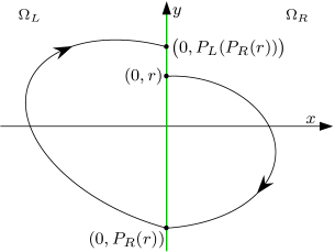
Figure 4.1: An illustration of the Poincaré map $P=P_{L}\circ P_{R}$ (defined more precisely in later sections subject to different assumptions) for a Filippov system of the form (3.1).

4.1 Key principles from analysis

The Picard-Lindelöf theorem Me07 tells us that if $F$ is Lipschitz then for any initial point $(x,y)$, (4.1) has a unique solution $\phi_{t}(x,y)$ on some time interval $(a,b)$ containing $0$. That is, $\phi_{0}(x,y)=(x,y)$ and $\dot{\phi}_{t}(x,y)=F(\phi_{t}(x,y))$ for all $t\in(a,b)$. If $F$ is $C^{k}$ then this smoothness is exhibited by $\phi_{t}$ Ha02 :

Lemma 4.1.

If $F$ is a $C^{k}$ ($k\geq 1$) function of $x$ and $y$, then $\phi_{t}(x,y)$ is a $C^{k}$ function of $x$, $y$, and $t$.

Actually an extra time derivative is available because $\phi_{t}$ can be written as an integral of $F$ over time, but we do not utilise this here. Return maps share the same degree of differentiability as $\phi_{t}$, as long as orbits intersect the Poincaré section transversally. This is a simple consequence of the implicit function theorem, here stated for a real-valued function $h(u,v)$.

Theorem 4.2 (Implicit function theorem (IFT)).

Suppose $h:\mathbb{R}\times\mathbb{R}^{m}\to\mathbb{R}$ is $C^{k}$, with $h(0,0)=0$ and $\frac{\partial h}{\partial u}(0,0)\neq 0$. Then there exists a neighbourhood $V\subset\mathbb{R}^{m}$ of $0$ and a unique $C^{k}$ function $\xi:V\to\mathbb{R}$ such that $h(\xi(v),v)=0$ for all $v\in V$.

The IFT tells us we can solve $h(u,v)=0$ for $u$, the solution being $u=\xi(v)$. As indicated in Fig. 4.1, given $r\in\mathbb{R}$ let $P_{R}(r)$ be the $y$-value of the next intersection of the forward orbit of $(0,r)$ with $x=0$ (if the orbit never returns to $x=0$ leave $P_{R}(r)$ undefined). Also write $\phi_{t}=(\varphi_{t},\psi_{t})$ (so that $\varphi_{t}$ and $\psi_{t}$ denote the $x$ and $y$-components of $\phi_{t}$ respectively). Then $P_{R}(r)=\psi_{t}(0,r)$, where $t>0$ is defined via $\varphi_{t}(0,r)=0$. The following result follows from the smoothness of the flow and the IFT (the conditions $f(0,r)\neq 0$ and $f(0,P_{R}(r))\neq 0$ ensure the orbit intersects $x=0$ transversally).

Lemma 4.3.

Suppose $F$ is $C^{k}$ ($k\geq 1$). If $P_{R}(r)$ is well-defined, $f(0,r)\neq 0$, and $f(0,P_{R}(r))\neq 0$, then $P_{R}(r)$ is $C^{k}$ at $r$.

Throughout this paper we use big-O and little-o notation to describe higher order terms in series expansions De81 . For functions $G,H:\mathbb{R}^{m}\to\mathbb{R}$ these are defined as follows: if ${\displaystyle\limsup_{z\to 0}\mathopen{}\mathclose{{}\left|\tfrac{G(z)}{H(z)}}\right|}$ is bounded then $G(z)=O(H(z))$, and if ${\displaystyle\lim_{z\to 0}\tfrac{G(z)}{H(z)}=0}$ then $G(z)=o(H(z))$. For example,

$${\rm e}^{z}=1+z+\tfrac{1}{2}z^{2}+O\mathopen{}\mathclose{{}\left(z^{3}}\right)=1+z+\tfrac{1}{2}z^{2}+o\mathopen{}\mathclose{{}\left(z^{2}}\right).$$

For multi-variable series ($m\geq 2$) we usually use some power of the $1$-norm of $z$ for the function $H$.

4.2 The return map about a focus

Here we consider (4.1) assuming

$$f(0,0)=g(0,0)=0,$$ (4.2)

so that the origin is an equilibrium. We suppose that the eigenvalues associated with the origin are complex:

$${\rm eig}({\rm D}F(0,0))=\lambda\pm{\rm i}\omega,\quad{\rm with~{}}\lambda\in\mathbb{R},\omega>0.$$ (4.3)

If $\lambda\neq 0$ then the origin is a focus, but here we also allow $\lambda=0$.

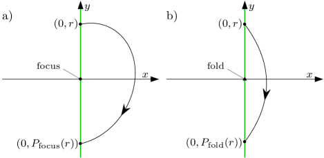
Figure 4.2: Typical orbits associated with the return maps $P_{\rm focus}$ (4.7) (where the origin is a focus) and $P_{\rm fold}$ (4.14) (where the origin is an invisible fold).

For any $r>0$, let $P_{\rm focus}(r)$ be the $y$-value of the next intersection of the forward orbit of $(0,r)$ with $x=0$, see Fig. 4.2-a. This is well-defined for small values of $r$. Also let $T_{\rm focus}(r)$ denote the corresponding evolution time. Thus the flow $\phi_{t}(x,y)$ satisfies

$$\phi_{T_{\rm focus}(r)}(0,r)=\mathopen{}\mathclose{{}\left(0,P_{\rm focus}(r)}\right).$$

We could assume orbits rotate clockwise, so that the corresponding orbits evolve in $x>0$ as discussed above, but this assumption is not required here. To state $P_{\rm focus}$ to second order we write

$${\rm D}F(0,0)=\begin{bmatrix}a_{1}&a_{2}\\ b_{1}&b_{2}\end{bmatrix},$$ (4.4)

and let

$$\chi_{\rm focus} =\frac{1}{\mathopen{}\mathclose{{}\left(\lambda^{2}+\omega^{2}}\right)\mathopen{}\mathclose{{}\left(\lambda^{2}+9\omega^{2}}\right)}\bigg{(}k_{1}\frac{\partial^{2}f}{\partial x^{2}}+k_{2}\frac{\partial^{2}f}{\partial x\partial y}$$

$$\quad+k_{3}\frac{\partial^{2}f}{\partial y^{2}}+\ell_{1}\frac{\partial^{2}g}{\partial x^{2}}+\ell_{2}\frac{\partial^{2}g}{\partial x\partial y}+\ell_{3}\frac{\partial^{2}g}{\partial y^{2}}\bigg{)}\bigg{|}_{x=y=0}\,,$$ (4.5)

where

$$\begin{split}k_{1}&=-a_{2}\mathopen{}\mathclose{{}\left(2a_{1}b_{2}-3a_{2}b_{1}-b_{2}^{2}}\right),\\ k_{2}&=-a_{2}b_{1}(4a_{1}+b_{2})+a_{1}b_{2}(2a_{1}-b_{2}),\\ k_{3}&=\frac{b_{1}(2a_{1}^{2}+7a_{1}b_{2}-3a_{2}b_{1})}{2}-\frac{b_{2}^{2}(2a_{1}^{2}-a_{1}b_{2}+a_{2}b_{1})}{2a_{2}},\\ \ell_{1}&=-a_{2}^{2}(a_{1}+b_{2}),\\ \ell_{2}&=a_{2}(2a_{1}^{2}-a_{1}b_{2}+3a_{2}b_{1}),\\ \ell_{3}&=-\frac{a_{1}\mathopen{}\mathclose{{}\left(2a_{1}^{2}-3a_{1}b_{2}+b_{2}^{2}}\right)}{2}-\frac{a_{2}b_{1}\mathopen{}\mathclose{{}\left(5a_{1}-b_{2}}\right)}{2}.\end{split}$$ (4.6)

Lemma 4.4.

Consider (4.1) where $F$ is $C^{2}$. Suppose (4.2) and (4.3) are satisfied. Then

$$P_{\rm focus}(r) =-{\rm e}^{\frac{\lambda\pi}{\omega}}r+{\rm e}^{\frac{\lambda\pi}{\omega}}\mathopen{}\mathclose{{}\left({\rm e}^{\frac{\lambda\pi}{\omega}}+1}\right)\chi_{\rm focus}r^{2}$$

$$\quad+o\mathopen{}\mathclose{{}\left(r^{2}}\right),$$ (4.7)

$$T_{\rm focus}(r) =\frac{\pi}{\omega}+O(r).$$ (4.8)

Lemma 4.4 is proved in Appendix A via brute-force asymptotic expansions of the flow. The result is used in many places later in the paper, but the $r^{2}$-term in (4.7) is only required for HLBs 8 and 9.

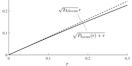
Figure 4.3: A numerical verification of Lemma 4.4 for the system (4.9).

As a simple demonstration of Lemma 4.4, consider the system

$$\begin{split}\dot{x}&=y-y^{2},\\ \dot{y}&=-x,\end{split}$$ (4.9)

for which $\lambda=0$ and $\omega=1$. Here $\chi_{\rm focus}=-\frac{2k_{3}}{9}$, where $k_{3}=-\frac{3}{2}$. By Lemma 4.5, $P_{\rm focus}(r)=-r+2\chi_{\rm focus}r^{2}+o\mathopen{}\mathclose{{}\left(r^{2}}\right)$. Fig. 4.3 shows $\sqrt{P_{\rm focus}(r)+r}$ (computed by numerically simulating (4.9)) and we observe that its slope at $r=0$ indeed appears to be $\sqrt{2\chi_{\rm focus}}$.

4.3 The return map about an invisible fold

Here we suppose

$$f(0,0) =0, \frac{\partial f}{\partial y}(0,0) >0, g(0,0) <0.$$ (4.10)

If we consider (4.1) only in $x>0$ and treat $x=0$ as a switching manifold, then the origin is an invisible fold (see Definition 3.3) about which orbits rotate clockwise.

For any $r>0$, let $P_{\rm fold}(r)$ be the $y$-value of the next intersection of the forward orbit of $(0,r)$ with $x=0$, see Fig. 4.2-b, and let $T_{\rm fold}(r)$ denote the corresponding evolution time. These are well-defined for sufficiently small values of $r>0$. A brief calculation reveals that maximum $x$-value attained by the orbit travelling from $(0,r)$ to $\mathopen{}\mathclose{{}\left(0,P_{\rm fold}(r)}\right)$ is $\frac{\frac{\partial f}{\partial y}(0,0)}{2|g(0,0)|}\,y^{2}+O\mathopen{}\mathclose{{}\left(y^{3}}\right)$. For this reason it is helpful to perform asymptotic expansions in $\sqrt{x}$ and $y$, and so we write

$$\begin{split}f(x,y)&=a_{1}x+a_{2}y+a_{5}y^{2}+O\mathopen{}\mathclose{{}\left(\mathopen{}\mathclose{{}\left(\sqrt{x}+|y|}\right)^{3}}\right),\\ g(x,y)&=b_{0}+b_{2}y+O\mathopen{}\mathclose{{}\left(\mathopen{}\mathclose{{}\left(\sqrt{x}+|y|}\right)^{2}}\right),\end{split}$$ (4.11)

where the coefficients have been labelled in a way that is consistent with other expressions in this paper. Notice $a_{2}>0$ and $b_{0}<0$ by (4.10). Let

$$\sigma_{\rm fold}=\frac{a_{1}}{b_{0}}+\frac{b_{2}}{b_{0}}-\frac{a_{5}}{a_{2}},$$ (4.12)

and

$$\chi_{\rm fold} =-\frac{a_{1}(a_{1}+b_{2})(a_{1}+2b_{2})}{b_{0}^{3}}+\frac{(a_{1}+b_{2})(4a_{1}+3b_{2})}{b_{0}^{2}}\,\sigma_{\rm fold}-\frac{5(a_{1}+b_{2})}{b_{0}}\,\sigma_{\rm fold}^{2}+\frac{40}{9}\,\sigma_{\rm fold}^{3}$$

$$\quad+\bigg{[}\frac{1}{b_{0}}\mathopen{}\mathclose{{}\left(\frac{a_{1}}{b_{0}}-\frac{a_{5}}{a_{2}}}\right)\frac{\partial^{2}f}{\partial x\partial y}-\frac{1}{6a_{2}}\mathopen{}\mathclose{{}\left(\frac{2a_{1}}{b_{0}}+\frac{2b_{2}}{b_{0}}-\frac{5a_{5}}{a_{2}}}\right)\frac{\partial^{3}f}{\partial y^{3}}+\frac{a_{2}}{b_{0}^{2}}\mathopen{}\mathclose{{}\left(\frac{a_{1}}{b_{0}}+\frac{b_{2}}{b_{0}}}\right)\frac{\partial g}{\partial x}$$

$$\quad+\frac{1}{2b_{0}}\mathopen{}\mathclose{{}\left(\frac{a_{1}}{b_{0}}-\frac{b_{2}}{b_{0}}-\frac{2a_{5}}{a_{2}}}\right)\frac{\partial^{2}g}{\partial y^{2}}-\frac{a_{2}}{b_{0}^{2}}\,\frac{\partial^{2}f}{\partial x^{2}}+\frac{1}{2b_{0}}\,\frac{\partial^{3}f}{\partial x\partial y^{2}}-\frac{1}{8a_{2}}\,\frac{\partial^{4}f}{\partial y^{4}}-\frac{a_{2}}{b_{0}^{2}}\,\frac{\partial^{2}g}{\partial x\partial y}+\frac{1}{2b_{0}}\,\frac{\partial^{3}g}{\partial y^{3}}\bigg{]}\bigg{|}_{x=y=0}\,.$$ (4.13)

Lemma 4.5.

Consider (4.1) where $F$ is $C^{5}$ and suppose (4.10) is satisfied. Then

$$P_{\rm fold}(r) =-r+\frac{2\sigma_{\rm fold}}{3}\,r^{2}-\frac{4\sigma_{\rm fold}^{2}}{9}\,r^{3}+\frac{2\chi_{\rm fold}}{15}\,r^{4}$$

$$\quad+o\mathopen{}\mathclose{{}\left(r^{4}}\right),$$ (4.14)

$$T_{\rm fold}(r) =\frac{-2}{b_{0}}\,r+O\mathopen{}\mathclose{{}\left(r^{2}}\right).$$ (4.15)

Lemma 4.5 is proved in Appendix A via brute-force asymptotic expansions, except, for brevity, we have only stated enough terms to obtain $P_{\rm fold}$ to second order. The full expression (4.14) is obtained by simply including more terms in the expansions. Indeed, while Lemma 4.5 is used below in several places, the $r^{4}$-term in (4.14) is only required for HLB 10.

It is interesting to note that quantity $\frac{P_{\rm fold}(r)+r}{r}$ has the same form as the Poincaré map associated with a Hopf bifurcation, or a perturbed centre more generally AnLe71 ; DuLl06 . For (4.14) the $O\mathopen{}\mathclose{{}\left(\mathopen{}\mathclose{{}\left(\sqrt{x}+|y|}\right)^{2}}\right)$ terms in $f$ and $O\mathopen{}\mathclose{{}\left(\mathopen{}\mathclose{{}\left(\sqrt{x}+|y|}\right)^{1}}\right)$ terms in $g$ behave like linear terms and determine the value of $\sigma_{\rm fold}$. If $\sigma_{\rm fold}=0$, then the $r^{2}$ and $r^{3}$ terms of (4.14) are both zero in the same way that the first non-zero Lyapunov constant of a perturbed centre corresponds to an odd power of $r$. For this reason the next two orders of terms contribute to the value of $\chi_{\rm fold}$, and so, in particular, both $\frac{\partial g}{\partial x}$ and $\frac{\partial^{4}f}{\partial y^{4}}$ appear in (4.13).

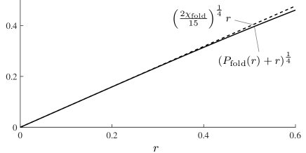
Figure 4.4: A numerical verification of Lemma 4.5 for the system (4.16).

As a minimal example, consider

$$\begin{split}\dot{x}&=y-y^{4},\\ \dot{y}&=-1,\end{split}$$ (4.16)

for which $\sigma_{\rm fold}=0$ and $\chi_{\rm fold}=3$. By Lemma 4.5, $P_{\rm fold}(r)=-r+\frac{2\chi_{\rm fold}}{15}\,r^{4}+o\mathopen{}\mathclose{{}\left(r^{4}}\right)$. Fig. 4.4 shows $\mathopen{}\mathclose{{}\left(P_{\rm fold}(r)+r}\right)^{\frac{1}{4}}$ (obtained by numerical simulation) and its linear appromixation.

4.4 The return map for an affine system

Here we suppose (4.1) has the form

$$\begin{bmatrix}\dot{x}\\ \dot{y}\end{bmatrix}=\begin{bmatrix}a_{1}x+a_{2}y\\ b_{0}+b_{1}x+b_{2}y\end{bmatrix},$$ (4.17)

and derive a return map on $x=0$ assuming that the Jacobian matrix

$$A=\begin{bmatrix}a_{1}&a_{2}\\ b_{1}&b_{2}\end{bmatrix},$$ (4.18)

has complex eigenvalues:

$${\rm eig}(A)=\lambda\pm{\rm i}\omega,\quad{\rm with~{}}\lambda\in\mathbb{R},\omega>0.$$ (4.19)

The formulas obtained here are used in several places below. This is because the dynamics near a BEB are well-approximated by a piecewise-linear system, meaning each smooth component is affine (linear plus a constant term). For the affine systems below, we are always able to find a coordinate change that removes the constant term in the $\dot{x}$ equation, as in (4.17). For HLBs 2 and 13 we require the eigenvalues of $A$ to be real-valued. This is remedied by using a purely imaginary value for $\omega$, but here we assume $\omega>0$.

The assumption $\omega>0$ ensures $A$ is invertible, and so (4.17) has the unique equilibrium

$$\begin{bmatrix}x^{*}\\ y^{*}\end{bmatrix}=\frac{\kappa}{\omega}\begin{bmatrix}a_{2}\\ -a_{1}\end{bmatrix},$$ (4.20)

where

$$\kappa=\frac{b_{0}\omega}{\lambda^{2}+\omega^{2}}.$$ (4.21)

Since the $\dot{x}$ equation has no constant term and $a_{2}\neq 0$ (a consequence of $\omega>0$), if $b_{0}\neq 0$ then the system has a unique fold at the origin (treating $x=0$ as a switching manifold).

We now assume $a_{2}>0$, so that for any $r>0$ the forward orbit of $(0,r)$ immediately enters $x>0$. For any $r>0$, we let $P_{\rm affine}(r)$ be the $y$-value of the next intersection of the forward orbit of $(0,r)$ with $x=0$. If this orbit does not reintersect $x=0$ we say $P_{\rm affine}(r)$ is undefined. Also we let $T_{\rm affine}(r)$ denote the corresponding evolution time. The functions $P_{\rm affine}$ and $T_{\rm affine}$ depend on $a_{1}$, $a_{2}$, $b_{0}$, $b_{1}$, and $b_{2}$, but, as we will see, they are completely determined by the values of $\lambda$, $\omega$, and $b_{0}$. Accordingly we write $P_{\rm affine}(r;\lambda,\omega,b_{0})$ and $T_{\rm affine}(r;\lambda,\omega,b_{0})$.

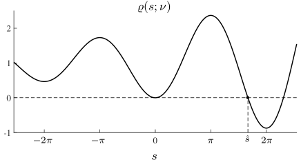
Figure 4.5: The auxiliary function (4.22) with $\nu=0.1$.

We cannot obtain an explicit closed form expression for $T_{\rm affine}$, so write $P_{\rm affine}$ and $T_{\rm affine}$ implicitly via the auxiliary function

$$\varrho(s;\nu)=1-{\rm e}^{\nu s}\mathopen{}\mathclose{{}\left(\cos(s)-\nu\sin(s)}\right),$$ (4.22)

which was used effectively in Chapter VIII of AnVi66 . Fig. 4.5 provides a plot of $\varrho(s;\nu)$ for a typical value of $\nu>0$. The function $\varrho$ attains its local maximum and minimum values at integer multiples of $\pi$ because

$$\frac{\partial\varrho}{\partial s}=\mathopen{}\mathclose{{}\left(1+\nu^{2}}\right){\rm e}^{\nu s}\sin(s).$$ (4.23)

For any $\nu>0$, we have $\varrho(s;\nu)>0$ for all nonzero $s\leq\pi$, and there exists unique $\hat{s}=\hat{s}(\nu)\in(\pi,2\pi)$ such that

$$\varrho(\hat{s};\nu)=0.$$ (4.24)

The case $\nu<0$ can be understood through the symmetry relation $\varrho(-s,-\nu)=\varrho(s,\nu)$.

Lemma 4.6.

Consider (4.17) with $a_{2}>0$ and $b_{0}\neq 0$, and suppose (4.19) is satisfied. For all $r>0$, $T=T_{\rm affine}(r;\lambda,\omega,b_{0})$ and $P=P_{\rm affine}(r;\lambda,\omega,b_{0})$ satisfy

$$r =\frac{-\kappa{\rm e}^{-\lambda T}\varrho\mathopen{}\mathclose{{}\left(\omega T;\frac{\lambda}{\omega}}\right)}{\sin(\omega T)},$$ (4.25)

$$P =\frac{\kappa{\rm e}^{\lambda T}\varrho\mathopen{}\mathclose{{}\left(\omega T;-\frac{\lambda}{\omega}}\right)}{\sin(\omega T)}.$$ (4.26)

If $b_{0}<0$ [$b_{0}>0$] then $\frac{dT}{dr}>0$ [$\frac{dT}{dr}<0$] for all $r>0$; also

$$\frac{dP}{dr}=\frac{r}{P}\,{\rm e}^{2\lambda T}.$$ (4.27)

As $r\to\infty$, $T\to\frac{\pi}{\omega}$ and $\frac{P}{r}\to-{\rm e}^{\frac{\lambda\pi}{\omega}}$.

1. If $b_{0}<0$, then as $r\to 0$, $T\to 0$ and $P\to 0$.

2. If $b_{0}>0$ and $\lambda<0$, let $\hat{r}=-\frac{b_{0}}{\omega}\,{\rm e}^{\nu\hat{s}(\nu)}\sin\mathopen{}\mathclose{{}\left(\hat{s}(\nu)}\right)$, where $\nu=-\frac{\lambda}{\omega}$. Then $T(\hat{r})=\frac{\hat{s}(\nu)}{\omega}$, $P(\hat{r})=0$, and $P$ is undefined for $r\in(0,\hat{r})$ ($P$ is defined in all other cases).

3. If $b_{0}>0$ and $\lambda>0$, then as $r\to 0$, $T\to\frac{\hat{s}(\nu)}{\omega}$ and $P\to\frac{b_{0}}{\omega}\,{\rm e}^{\nu\hat{s}(\nu)}\sin\mathopen{}\mathclose{{}\left(\hat{s}(\nu)}\right)$, where $\nu=\frac{\lambda}{\omega}$.

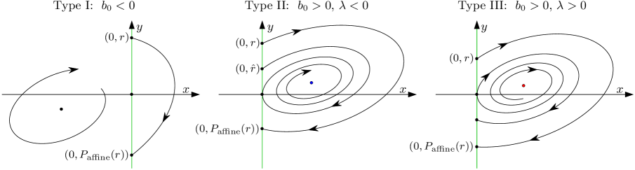
Figure 4.6: Phase portraits of the affine system (4.17). The return map $P_{\rm affine}$ conforms to one of three types, see Lemma 4.6.

Lemma 4.6 is proved in Appendix A via direct calculations. There are three cases for the qualitative nature of $T_{\rm affine}$ and $P_{\rm affine}$, see Fig. 4.6 (this ignores the special case $\lambda=0$). If $b_{0}<0$, we say $T_{\rm affine}$ and $P_{\rm affine}$ are of Type I. The equilibrium $(x^{*},y^{*})$ lies in $x<0$, so $(x^{*},y^{*})$ is virtual and the origin is an invisible fold (in the context of the Filippov system (3.1)). If $b_{0}>0$ and $\lambda<0$, we say $T_{\rm affine}$ and $P_{\rm affine}$ are of Type II. Here $(x^{*},y^{*})$ is an admissible stable focus and the origin is a visible fold. For all $r\in(0,\hat{r})$, $P_{\rm affine}$ is undefined because the forward orbit of $(0,r)$ converges to $(x^{*},y^{*})$ without reintersecting $x=0$. Finally if $b_{0}>0$ and $\lambda>0$, we say $T_{\rm affine}$ and $P_{\rm affine}$ are of Type III. Here $(x^{*},y^{*})$ is an admissible unstable focus and the origin is a visible fold.

Lemma 4.6 assumes $b_{0}\neq 0$. If $b_{0}=0$, then $P_{\rm affine}$ and $T_{\rm affine}$ are well-defined, but the formulas (4.25) and (4.26) are ill-posed because they are of the form $\frac{0}{0}$. In this case we can use Lemma 4.4. Taking $r\to\infty$ is analogous to taking $b_{0}\to 0$, and for this reason the $r\to\infty$ asymptotics in Lemma 4.6 match the leading order terms of (4.7) and (4.8).

5 Boundary equilibrium bifurcations in continuous systems

Here we consider piecewise-smooth systems of the form

$$\begin{bmatrix}\dot{x}\\ \dot{y}\end{bmatrix}=\begin{cases}F_{L}(x,y;\mu),&x\leq 0,\\ F_{R}(x,y;\mu),&x\geq 0.\end{cases}$$ (5.1)

The non-strict inequalities mean that $F_{L}(0,y;\mu)=F_{R}(0,y;\mu)$, for all values of $y$ and $\mu$. That is (5.1) is continuous on $x=0$ and does not exhibit sliding motion.

As the value of $\mu$ is varied, a BEB (boundary equilibrium bifurcation) occurs when a regular equilibrium collides with $x=0$. For clarity, let us suppose the bifurcation occurs at the origin when $\mu=0$. For the continuous system (5.1), at $\mu=0$ the origin is a regular equilibrium of both left and right half-systems. Assuming certain genericity conditions are satisfied, each half-system has a unique regular equilibrium locally. Each equilibrium is admissible for either small $\mu<0$ or small $\mu>0$ (we say the equilibrium is admissible for ‘one sign of $\mu$’). Consequently there are two cases: the equilibria may be admissible for different signs of $\mu$ (called persistence because a single equilibrium appears to persist) or the same sign of $\mu$ (called a nonsmooth-fold as it resembles a saddle-node bifurcation) DiBu08 ; Si10 . The distance of each equilibrium from $x=0$ is asymptotically proportional to $|\mu|$.

Other invariant sets can be created in BEBs Le06 ; LeNi04 . These include limit cycles (as discussed below) and, for systems of three or more dimensions, chaotic sets DiNo08 ; Si16c . The diameter of all bounded invariant sets (except equilibria) is asymptotically proportional to $|\mu|$.

For two-dimensional systems, equilibria and limit cycles are the only possible bounded invariant sets and there are ten topologically distinct BEBs (assuming genericity). These can be grouped into the following five scenarios: (i) persistence with the equilibria being of the same stability, (ii) persistence with different stability, (iii) persistence with different stability and a limit cycle, (iv) nonsmooth-fold, and (v) nonsmooth-fold with a limit cycle, see Si10 ; SiMe12 . We view scenario (iii) as Hopf-like, for which there are two topologically distinct cases. Either both equilibria are foci, HLB 1, or one is a focus and the other is a node, HLB 2. In both cases one equilibrium is attracting and the other is repelling. For HLB 1, the stability of the limit cycle is determined by the sign of $\frac{\lambda_{L}}{\omega_{L}}+\frac{\lambda_{R}}{\omega_{R}}$, where the eigenvalues associated with the equilibria are $\lambda_{L}\pm{\rm i}\omega_{L}$ and $\lambda_{R}\pm{\rm i}\omega_{R}$. For HLB 2, the stability of the limit cycle is the same as that of the node. In both cases the stability of the limit cycle is the same as the stability of the origin when $\mu=0$ (an important stability problem for many switched control systems CaHe03 ; DiCa05 ).

In a neighbourhood of a BEB, the system is approximately piecewise-linear. The local behaviour of the BEB is in part governed by global properties of the piecewise-linear approximation. As a result, in the limit $\mu\to 0$ the limit cycle for HLBs 1 and 2 is a rather irregular union of orbit segments of the left and right half-systems. Also the formula for the period of the limit cycle is not simple and can only be stated implicitly, see (5.7).

The earliest rigorous analyses of HLBs appear to be for piecewise-linear systems. In Chapter VIII of AnVi66 a limit cycle is identified in a piecewise-linear model of a valve generator by constructing a Poincaré map (there called a point transformation) and using the auxiliary function $\varrho$ (4.22). This model is actually Filippov; it is given below as an example in §6.2 and described also in Ye86 .

Motivated by circuit systems Ch94 ; ChDe86 , Lum and Chua LuCh91 performed an extensive analysis of two-dimensional piecewise-linear continuous ODE systems. For certain scenarios they were able to prove the existence of an attracting annulus and conjectured that within the annulus there exists a unique stable limit cycle. This was subsequently proved by Friere and coworkers in FrPo98 by reducing the number of parameters in the equations, using the function $\varrho$, and meticulously considering all possible cases for the nature of the equilibria. For piecewise-linear systems they established HLB 1 in FrPo97 and HLB 2 in FrPo98 .

If (5.1) is not piecewise-linear, then robust dynamics of its piecewise-linear approximation are exhibited by (5.1) near the BEB DiBu08 ; Si10 . Intuitively, hyperbolic limit cycles are robust phenomena, but this needs to be proved. This was achieved in SiMe07 by demonstrating that the limit cycle can be expressed as a hyperbolic fixed point of a smooth Poincaré map, except their proof lacks the necessary scaling to apply the IFT correctly (this is fixed in the proof in Appendix B).

5.1 The focus/focus case — HLB 1

For each $J\in\{L,R\}$, we write

$$F_{J}(x,y;\mu)=\begin{bmatrix}f_{J}(x,y;\mu)\\ g_{J}(x,y;\mu)\end{bmatrix},$$ (5.2)

and suppose

$$f_{J}(0,0;0)=g_{J}(0,0;0)=0,$$ (5.3)

so that the origin is a boundary equilibrium when $\mu=0$. We suppose the origin is an unstable focus of the left half-system and a stable focus of the right half-system, that is

$$\begin{split}{\rm eig}({\rm D}F_{L}(0,0;0))&=\lambda_{L}\pm{\rm i}\omega_{L}\,,\quad{\rm with~{}}\lambda_{L}>0,\omega_{L}>0,\\ {\rm eig}({\rm D}F_{R}(0,0;0))&=\lambda_{R}\pm{\rm i}\omega_{R}\,,\quad{\rm with~{}}\lambda_{R}<0,\omega_{R}>0.\\ \end{split}$$ (5.4)

Locally each half-system has a unique equilibrium with an $x$-value equal to $\frac{-\beta\mu}{\lambda_{J}^{2}+\omega_{J}^{2}}+O\mathopen{}\mathclose{{}\left(\mu^{2}}\right)$, where

$$\beta=\mathopen{}\mathclose{{}\left(\frac{\partial f_{L}}{\partial\mu}\frac{\partial g_{L}}{\partial y}-\frac{\partial g_{L}}{\partial\mu}\frac{\partial f_{L}}{\partial y}}\right)\bigg{|}_{x=y=\mu=0}.$$ (5.5)

Here we have used the continuity of (5.1) (the derivatives of $F_{L}$ in (5.5) are the same for $F_{R}$). Consequently $\beta\neq 0$ is the transversality condition for HLB 1. Below we assume $\beta>0$ without loss of generality. As mentioned above the stability of the limit cycle emanating from the origin is determined by the sign of

$$\alpha=\frac{\lambda_{L}}{\omega_{L}}+\frac{\lambda_{R}}{\omega_{R}}.$$ (5.6)

Recall $\Omega_{L}$ and $\Omega_{R}$ denote the left and right half-planes, see (3.2).

Theorem 5.1 (HLB 1).

Consider (5.1) where $F_{L}$ and $F_{R}$ are $C^{2}$. Suppose (5.3) and (5.4) are satisfied and $\beta>0$. In a neighbourhood of $(x,y;\mu)=(0,0;0)$,

1. there exists a unique stationary solution: a stable focus in $\Omega_{R}$ for $\mu<0$, and an unstable focus in $\Omega_{L}$ for $\mu>0$,

2. if $\alpha<0$ [$\alpha>0$] there exists a unique stable [unstable] limit cycle for $\mu>0$ [$\mu<0$], and no limit cycle for $\mu<0$ [$\mu>0$].

The minimum and maximum $x$ and $y$-values of the limit cycle are asymptotically proportional to $|\mu|$, and its period is $T=T_{L}+T_{R}+O(\mu)$ where $T_{L}$ and $T_{R}$ satisfy

$$\begin{split}\frac{\omega_{L}G\mathopen{}\mathclose{{}\left(\omega_{L}T_{L};-\frac{\lambda_{L}}{\omega_{L}}}\right)}{\lambda_{L}^{2}+\omega_{L}^{2}}+\frac{\omega_{R}G\mathopen{}\mathclose{{}\left(\omega_{R}T_{R};\frac{\lambda_{R}}{\omega_{R}}}\right)}{\lambda_{R}^{2}+\omega_{R}^{2}}&=0,\\ \frac{\omega_{L}G\mathopen{}\mathclose{{}\left(\omega_{L}T_{L};\frac{\lambda_{L}}{\omega_{L}}}\right)}{\lambda_{L}^{2}+\omega_{L}^{2}}+\frac{\omega_{R}G\mathopen{}\mathclose{{}\left(\omega_{R}T_{R};-\frac{\lambda_{R}}{\omega_{R}}}\right)}{\lambda_{R}^{2}+\omega_{R}^{2}}&=0,\end{split}$$ (5.7)

and $G(s;\nu)=\frac{{\rm e}^{-\nu s}\varrho(s;\nu)}{\sin(s)}$, where $\varrho$ is the auxiliary function (4.22).

HLB 1 is exhibited by the McKean neuron model: a piecewise-linear version of the Fitzhugh-Nagumo model for an excitable neuron Mc70 . Following Co08 we write the model as

$$\begin{split}\dot{v}&=q(v)-w+I,\\ \dot{w}&=b(v-cw),\end{split}$$ (5.8)

where $v$ represents membrane voltage, $w$ is an effective gating variable, and

$$q(v)=\begin{cases}-v,&v\leq\frac{a}{2},\\ v-a,&\frac{a}{2}\leq v\leq\frac{a+1}{2},\\ 1-v,&v\geq\frac{a+1}{2}.\end{cases}$$ (5.9)

The function $q$ mimics the cubic caricature of the Fitzhugh-Nagumo model. The McKean model is one of many piecewise-linear models of neuron dynamics. As a general rule the dynamics of these models may not match experimentally observed dynamics with as much quantitative accuracy as more sophisticated high-dimensional models, but they often fit qualitatively and are amenable to an exact analysis DeGu16 ; RoCo12 ; ToGe03 . This is particularly helpful for understanding neural networks Co08 ; CoLa18 ; CoTh16 .

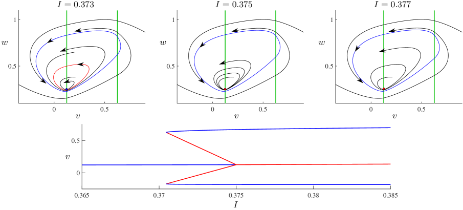
Figure 5.1: An illustration of HLB 1 for the McKean neuron model (5.8) with (5.10). By decreasing the value of $I$ an unstable focus collides with the switching manifold $v=\frac{a}{2}$ when $I=0.375$ where it turns into a stable focus and emits an unstable limit cycle. The limit cycle subsequently undergoes a saddle-node bifurcation and becomes a stable relaxation oscillation.

Here we treat the external stimulus $I$ as a bifurcation parameter. With the remaining parameter values fixed at

$$a=0.25,\qquad b=0.5,\qquad c=0.5,$$ (5.10)

a subcritical HLB 1 occurs at $I=0.375$, see Fig. 5.1. As the value of $I$ is decreased through $I=0.375$ an unstable focus in $\frac{a}{2}<v<\frac{a+1}{2}$ collides with the switching manifold $v=\frac{a}{2}$ when $I=0.375$ and transitions to a stable focus in $v<\frac{a}{2}$. The eigenvalues associated with the foci are $0.3750\pm 0.3307{\rm i}$ and $-0.6250\pm 0.5995{\rm i}$ (to four decimal places). Thus $\alpha\approx 0.0913>0$ and so an unstable limit cycle is created. As the value of $I$ is decreased further, the unstable limit cycle undergoes a grazing bifurcation with the other switching manifold, $v=\frac{a+1}{2}$, and is very shortly followed by a saddle-node bifurcation at which the limit cycle collides and annihilates with a coexisting stable limit cycle. In summary, a subcritical HLB 1 and a saddle-node bifurcation of limit cycles bound a small interval of bistability. With smaller values of $b$ the McKean model exhibits HLB 2.

5.2 The focus/node case — HLB 2

We now suppose that the origin is a stable node of the right half-system when $\mu=0$. We write the eigenvalues as

$$\begin{split}{\rm eig}({\rm D}F_{L}(0,0;0))&=\lambda_{L}\pm{\rm i}\omega_{L}\,,\quad{\rm with~{}}\lambda_{L}>0,\omega_{L}>0,\\ {\rm eig}({\rm D}F_{R}(0,0;0))&=\lambda_{R}\pm\eta_{R}\,,\quad{\rm with~{}}0<\eta_{R}<-\lambda_{R}\,.\end{split}$$ (5.11)

Theorem 5.2 (HLB 2).

Consider (5.1) where $F_{L}$ and $F_{R}$ are $C^{2}$. Suppose (5.3) and (5.11) are satisfied and $\beta>0$. In a neighbourhood of $(x,y;\mu)=(0,0;0)$,

1. there exists a unique stationary solution: a stable node in $\Omega_{R}$ for $\mu<0$, and an unstable focus in $\Omega_{L}$ for $\mu>0$,

2. there exists a unique stable limit cycle for $\mu>0$, and no limit cycle for $\mu<0$.

The minimum and maximum $x$ and $y$-values of the limit cycle are asymptotically proportional to $\mu$, and its period is $T=T_{L}+T_{R}+O(\mu)$ where $T_{L}$ and $T_{R}$ satisfy (5.7) using $\omega_{R}={\rm i}\eta_{R}$.

Notice how Theorem 5.2 contains no criticality constant $\alpha$. The stability of the limit cycle is determined from our assumption that the focus is unstable and the node is stable. The case of a stable focus and an unstable node (giving an unstable limit cycle) can be treated via time-reversal.

To illustrate HLB 2 we consider the reduced ocean circulation model of RoSa17 :

$$\begin{split}\dot{\bar{y}}&=\bar{\mu}-\bar{y}-A\bar{y}|\bar{y}-1|,\\ \dot{\bar{\mu}}&=\delta_{0}(\lambda-\bar{y}).\end{split}$$ (5.12)

This is equation (18) of RoSa17 except bars have been added to the variables to avoid confusion with the present notation. The variable $\bar{y}$ represents the difference in the salinity of the ocean near the equator from that near the poles, and $\bar{\mu}$ is a forcing ratio. The parameters $\lambda$, $A$, and $\delta_{0}$ each take positive real values.

The model is a reduced version of a box model of ocean circulation developed by Stommel St61 . The circulation is assumed to occur between two regions (boxes): one equatorial and one polar. The regions are assumed to be well-mixed, so the dynamics in the regions is assumed to depend on the magnitude of the circulation, but not its direction. This manifests as $|\bar{y}-1|$ in (5.12) making the model piecewise-smooth.

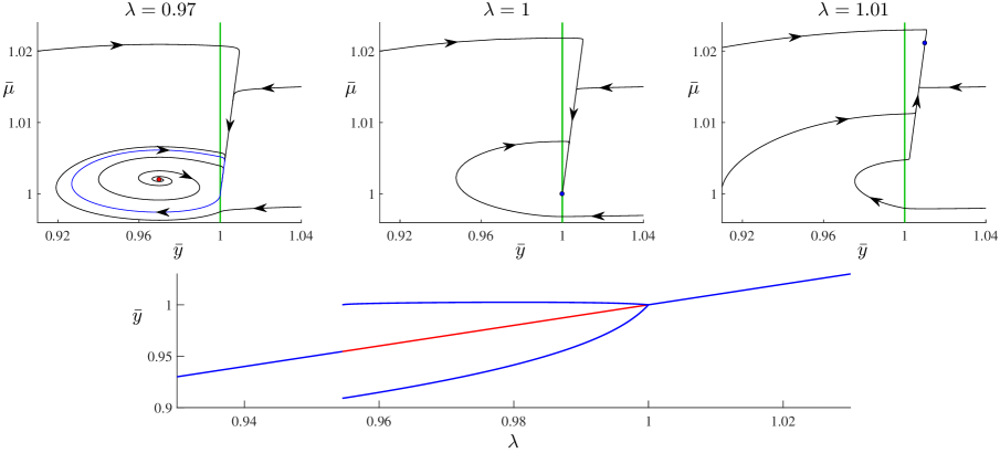
Figure 5.2: An illustration of HLB 2 for ocean circulation model (5.12) with $A=1.1$ and $\delta_{0}=0.01$. By decreasing the value of $\lambda$ a stable node collides with the switching manifold $\bar{y}=1$ when $\lambda=1$ where it turns into an unstable focus and emits a stable limit cycle.

The system exhibits a BEB when $\lambda=1$, see Fig. 5.2. With $\lambda>1$ there is a stable node in $\bar{y}>1$, and if $1<A<1+2\sqrt{\delta_{0}}$, then with $\lambda<1$ there is an unstable focus in $\bar{y}<1$. In this case an instance of HLB 2 occurs at $\lambda=1$ and so a stable limit cycle is created. For the parameter values of Fig. 5.2, the focus subsequently changes stability at $\lambda=\frac{21}{22}\approx 0.9545$. Here the limit cycle is destroyed in a degenerate fashion (at $\lambda=\frac{21}{22}$ there exists an uncountable family of periodic orbits). If the value of $A$ is increased past $1+2\sqrt{\delta_{0}}$ the unstable focus changes to an unstable node and a large amplitude limit cycle is created in the BEB at $\lambda=1$. Related to this, HLB 2 has been well-documented in PWL systems in the context of canards DeFr13 ; FeDe16 ; PoRo15 ; SiKu11 .

6 Boundary equilibrium bifurcations in Filippov systems

Here we consider Filippov systems of the form

$$\begin{bmatrix}\dot{x}\\ \dot{y}\end{bmatrix}=\begin{cases}F_{L}(x,y;\mu),&x<0,\\ F_{R}(x,y;\mu),&x>0,\end{cases}$$ (6.1)

and write

$$F_{J}(x,y;\mu)=\begin{bmatrix}f_{J}(x,y;\mu)\\ g_{J}(x,y;\mu)\end{bmatrix},$$ (6.2)

for each $J\in\{L,R\}$.

Let us suppose an equilibrium of the left half-system collides with $x=0$ at the origin when $\mu=0$. Since $F_{L}$ and $F_{R}$ are essentially independent, we would expect that the origin is not an equilibrium of the right half-system when $\mu=0$. In this way, generic BEBs of Filippov systems are different to those of continuous systems (described in §5). But as with continuous systems locally there are exactly two equilibria: the regular equilibrium and a pseudo-equilibrium, and these coincide at the bifurcation. The equilibria are either admissible for different signs of $\mu$ (persistence) or the same sign of $\mu$ (nonsmooth-fold) DiBu08 ; Si18d . The distance of each equilibrium from the origin, and the diameter of any other bounded invariant set created in the bifurcation, is asymptotically proportional to $|\mu|$.

For two-dimensional systems there are $12$ topologically distinct BEBs (assuming genericity) Gl16d ; HoHo16 . Of these, only one is Hopf-like in that it corresponds to persistence and creates a local limit cycle. This is HLB 3, called ${\rm BF}_{3}$ in KuRi03 , see §6.1. In §6.2 we consider the degenerate case that the origin is also an equilibrium of the right half-system at $\mu=0$ (HLB 4) as this occurs in some applications.

6.1 The generic case — HLB 3

We suppose that the origin is an unstable focus of the left half-system of (6.1) when $\mu=0$, that is

$$f_{L}(0,0;0)=g_{L}(0,0;0)=0,$$ (6.3)

and

$${\rm eig}({\rm D}F_{L}(0,0;0))=\lambda_{L}\pm{\rm i}\omega_{L}\,,\quad{\rm with~{}}\lambda_{L}>0,\omega_{L}>0.$$ (6.4)

Locally the left half-system has a unique equilibrium with an $x$-value of $\frac{-\beta\mu}{\lambda_{L}^{2}+\omega_{L}^{2}}+O\mathopen{}\mathclose{{}\left(\mu^{2}}\right)$, where

$$\beta=\mathopen{}\mathclose{{}\left(\frac{\partial f_{L}}{\partial\mu}\frac{\partial g_{L}}{\partial y}-\frac{\partial g_{L}}{\partial\mu}\frac{\partial f_{L}}{\partial y}}\right)\bigg{|}_{x=y=\mu=0},$$ (6.5)

which is identical to (5.5).

Since $\lambda_{L}>0$, for a limit cycle to be created at $\mu=0$ we require $a_{0R}<0$ where

$$a_{0R}=f_{R}(0,0;0).$$ (6.6)

Then, near the origin, the switching manifold is the union of an attracting sliding region, a crossing region, and a fold (or boundary focus when $\mu=0$). By evaluating the sliding vector field (3.7) when $\mu=0$, we obtain $g_{\rm slide}(y;0)=\frac{\gamma}{-a_{0R}}\,y+O\mathopen{}\mathclose{{}\left(y^{2}}\right)$, where

$$\gamma=\mathopen{}\mathclose{{}\left(\frac{\partial f_{L}}{\partial y}g_{R}-\frac{\partial g_{L}}{\partial y}f_{R}}\right)\bigg{|}_{x=y=\mu=0}.$$ (6.7)

In the following theorem we assume $\gamma<0$ so that the BEB corresponds to persistence. If instead $\gamma>0$ then the BEB is a nonsmooth-fold and a limit cycle may be created, this is ${\rm BF}_{1}$ in KuRi03 . In some sense the case $\gamma>0$ occurs more naturally: if ${\rm D}F_{L}(0,0;0)$ is in real Jordan form and orbits in $\Omega_{R}$ approach $x=0$ at right angles to $x=0$, then $\gamma>0$. To have $\gamma<0$ the vector field $F_{R}$ needs to be directed so that it overcomes the instability produced by the unstable focus.

Theorem 6.1 (HLB 3).

Consider (6.1) where $F_{L}$ and $F_{R}$ are $C^{2}$. Suppose (6.3) and (6.4) are satisfied, $\beta>0$, $f_{R}(0,0;0)<0$, and $\gamma<0$. In a neighbourhood of $(x,y;\mu)=(0,0;0)$,

1. there exists a unique stationary solution: a stable pseudo-equilibrium for $\mu<0$, and an unstable focus in $\Omega_{L}$ for $\mu>0$,

2. there exists a unique stable limit cycle for $\mu>0$, and no limit cycle for $\mu<0$.

The minimum $x$-value and minimum and maximum $y$-values of the limit cycle are asymptotically proportional to $\mu$, and its period is $T=T_{L}+T_{\rm slide}+O(\mu)$ where

$$\begin{split}T_{L}&=\frac{1}{\omega_{L}}\,\hat{s}\mathopen{}\mathclose{{}\left(\frac{\lambda_{L}}{\omega_{L}}}\right),\\ T_{\rm slide}&=\frac{a_{0R}}{\gamma}\,\ln\mathopen{}\mathclose{{}\left(1-\frac{\gamma}{a_{0R}\omega_{L}}\,{\rm e}^{\frac{\lambda_{L}}{\omega_{L}}\,\hat{s}\mathopen{}\mathclose{{}\left(\frac{\lambda_{L}}{\omega_{L}}}\right)}\sin\mathopen{}\mathclose{{}\left(\hat{s}\mathopen{}\mathclose{{}\left(\frac{\lambda_{L}}{\omega_{L}}}\right)}\right)}\right),\end{split}$$ (6.8)

and $\hat{s}$ is defined in §4.4.

While HLB 3 has been well understood for some time through qualitative studies such as KuRi03 , the proof in Appendix B is possibly the first quantitative analysis of HLB 3 that accommodates nonlinear terms in $F_{L}$ and $F_{R}$. The limit cycle involves motion in $\Omega_{L}$ of duration $t_{L}(\mu)=T_{L}+O(\mu)$ and a segment of sliding motion of duration $t_{\rm slide}(\mu)=T_{\rm slide}+O(\mu)$. If (6.1) is piecewise-linear then $t_{L}(\mu)$ is independent of $\mu$ but $t_{\rm slide}(\mu)$ is, in general, not. This is because the sliding vector field (3.7) is nonlinear.

To illustrate HLB 3, we consider the predator-prey model of YaTa13 :

$$\begin{split}\dot{x}&=rx\mathopen{}\mathclose{{}\left(1-\frac{x}{K}}\right)-q(x)y,\\ \dot{y}&=\mathopen{}\mathclose{{}\left(kq(x)-\delta}\right)y,\end{split}$$ (6.9)

where $x(t)$ and $y(t)$ denote the prey and predator populations respectively. Also

$$q(x)=\begin{cases}0,&x<R_{c}\,,\\ \frac{bx}{1+bhx},&x>R_{c}\,,\end{cases}$$ (6.10)

and all other quantities are positive constants. In the limit $K\to\infty$ ($K$ is the carrying capacity of the prey) the system reduces to the Gause predator-prey model GaSm36 for which the prey is a yeast and the predator is a certain single-celled organism. The Gause model is Lotka-Volterra with a Holling type II functional response BrCa01 . It assumes that when the yeast population is below a threshold $R_{c}$ the yeast forms a sediment and cannot be consumed by the organisms. For this reason the model is Filippov. Interestingly its conception and initial study predates the fundamental work of Filippov Fi60 . For modern studies of the Gause model refer to Kr11 ; TaLi13 .

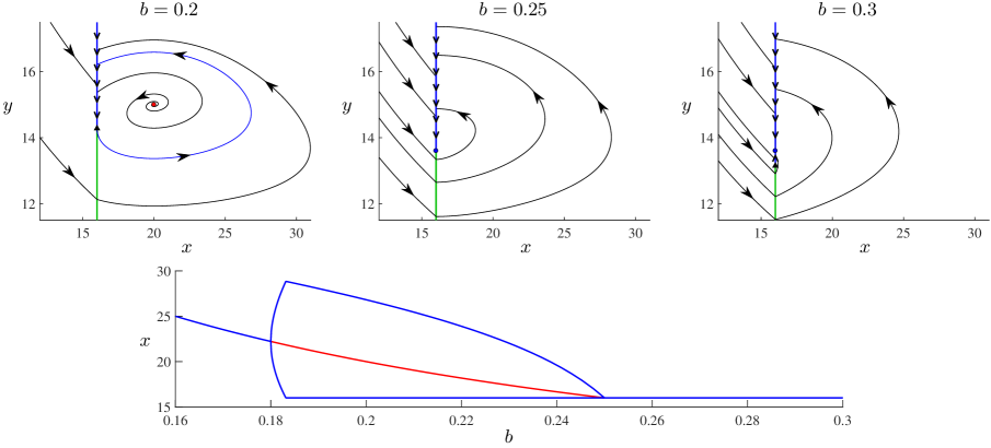
Figure 6.1: An illustration of HLB 3 for the Gause predator-prey model with finite prey carrying capacity, (6.9)–(6.11). By decreasing the value of $b$ a stable pseudo-equilibrium reaches a boundary of its sliding region when $b=0.25$ where it turns into an unstable focus and emits a stable limit cycle involving one sliding segment.

Fig. 6.1 illustrates the dynamics of (6.9) using

$$R_{c} =16, r =1, h =1,$$ (6.11)

$$k =0.45, \delta =0.36, K =50,$$

and $b$ as a bifurcation parameter. As the value of $b$ is decreased, a stable pseudo-equilibrium turns into an unstable focus at $b=0.25$ (an instance of HLB 3). The resulting limit cycle involves one segment of sliding motion until a grazing-sliding bifurcation DiKo02 ; DiKo03 ; JeHo11 occurs at $b\approx 0.1831$. The limit cycle is subsequently destroyed in a supercritical Hopf bifurcation at $b=0.18$.

6.2 A degenerate case — HLB 4

For (6.1) with $\mu=0$, we now suppose the origin is an unstable focus for the left half-system and a stable focus for the right half-system, that is

$$f_{L}(0,0;0)=g_{L}(0,0;0)=f_{R}(0,0;0)=g_{R}(0,0;0)=0,$$ (6.12)

and

$$\begin{split}{\rm eig}({\rm D}F_{L}(0,0;0))&=\lambda_{L}\pm{\rm i}\omega_{L}\,,\quad{\rm with~{}}\lambda_{L}>0,\omega_{L}>0,\\ {\rm eig}({\rm D}F_{R}(0,0;0))&=\lambda_{R}\pm{\rm i}\omega_{R}\,,\quad{\rm with~{}}\lambda_{R}<0,\omega_{R}>0.\end{split}$$ (6.13)

Locally, each half-system has a unique equilibrium (a focus) and its direction of rotation is determined by the sign of

$$a_{2J}=\frac{\partial f_{J}}{\partial y}(0,0;0).$$ (6.14)

If $a_{2J}>0$, rotation is clockwise; if $a_{2J}<0$, rotation is anticlockwise. Note that $a_{2J}\neq 0$ is a consequence of (6.13) and has the opposite sign to $\frac{\partial g_{J}}{\partial x}(0,0;0)$ (which could instead be used to characterise the direction of rotation). In order to have a Hopf-like bifurcation we assume $a_{2L}a_{2R}>0$ so that the foci have the same direction of rotation (for HLB 1 this property follows automatically from the continuity of the system on the switching manifold).

As in §5.1, let

$$\alpha=\frac{\lambda_{L}}{\omega_{L}}+\frac{\lambda_{R}}{\omega_{R}}.$$ (6.15)

Here we show that if $\alpha<0$ (so that the origin is stable when $\mu=0$) and, locally, there is no attracting sliding region when the unstable focus is admissible, then a unique stable limit cycle is created. We call this HLB 4; it generalises HLB 1 to Filippov systems. The analogous creation of an unstable limit cycle can be understood by reversing time. The assumption of no attracting sliding region is sufficient, but not necessary, to ensure uniqueness of the limit cycle. Without this assumption up to three limit cycles can be created simultaneously BrMe13 ; FrPo14 ; HuYa12b , see also HaZh10 ; HuYa13 ; HuYa14 .

The $x$-values of the foci are $\frac{-\beta_{J}\mu}{\lambda_{J}^{2}+\omega_{J}^{2}}+O\mathopen{}\mathclose{{}\left(\mu^{2}}\right)$, where

$$\beta_{J}=\mathopen{}\mathclose{{}\left(\frac{\partial f_{J}}{\partial\mu}\frac{\partial g_{J}}{\partial y}-\frac{\partial g_{J}}{\partial\mu}\frac{\partial f_{J}}{\partial y}}\right)\bigg{|}_{x=y=\mu=0}.$$ (6.16)

Thus the condition $\beta_{L}\beta_{R}>0$ ensures the foci are admissible for different signs of $\mu$. In view of the replacement $\mu\mapsto-\mu$, we assume $\beta_{L}>0$ and $\beta_{R}>0$. Then the unstable focus is admissible (in $\Omega_{L}$) when $\mu>0$.

Locally the left half-system has a unique visible fold when $\mu>0$. At this fold $f_{R}(0,y;\mu)=\frac{\gamma}{a_{2L}}\,\mu+O\mathopen{}\mathclose{{}\left(\mu^{2}}\right)$, where

$$\gamma=\mathopen{}\mathclose{{}\left(\frac{\partial f_{L}}{\partial y}\frac{\partial f_{R}}{\partial\mu}-\frac{\partial f_{L}}{\partial\mu}\frac{\partial f_{R}}{\partial y}}\right)\bigg{|}_{x=y=\mu=0}.$$ (6.17)

Hence if $a_{2L}\gamma>0$ then the fold bounds a crossing region and a repelling sliding region. Thus $a_{2L}\gamma>0$ produces the desired assumption for the absence of an attracting sliding region. This condition also accommodates the case $\alpha>0$ and below we also allow $\gamma=0$.

Theorem 6.2 (HLB 4).

Consider (6.1) where $F_{L}$ and $F_{R}$ are $C^{2}$. Suppose (6.12) and (6.13) are satisfied, $a_{2L}a_{2R}>0$, $\beta_{L}>0$, $\beta_{R}>0$, and $a_{2L}\gamma\geq 0$. In a neighbourhood of $(x,y;\mu)=(0,0;0)$,

1. there exists a stable focus in $\Omega_{R}$ for $\mu<0$, and an unstable focus in $\Omega_{L}$ for $\mu>0$,

2. if $\alpha<0$ [$\alpha>0$] there exists a unique stable [unstable] limit cycle for $\mu>0$ [$\mu<0$], and no limit cycle for $\mu<0$ [$\mu>0$].

The minimum and maximum $x$ and $y$-values of the limit cycle are asymptotically proportional to $|\mu|$, and its period is $T=T_{L}+T_{R}+O(\mu)$ where $T_{L}$ and $T_{R}$ satisfy

$$\begin{split}\frac{\gamma}{a_{2L}a_{2R}}&=\frac{\beta_{L}\omega_{L}}{a_{2L}\mathopen{}\mathclose{{}\left(\lambda_{L}^{2}+\omega_{L}^{2}}\right)}\,G\mathopen{}\mathclose{{}\left(\omega_{L}T_{L};-\frac{\lambda_{L}}{\omega_{L}}}\right)\\ &\quad+\frac{\beta_{R}\omega_{R}}{a_{2R}\mathopen{}\mathclose{{}\left(\lambda_{R}^{2}+\omega_{R}^{2}}\right)}\,G\mathopen{}\mathclose{{}\left(\omega_{R}T_{R};\frac{\lambda_{R}}{\omega_{R}}}\right),\\ \frac{-\gamma}{a_{2L}a_{2R}}&=\frac{\beta_{L}\omega_{L}}{a_{2L}\mathopen{}\mathclose{{}\left(\lambda_{L}^{2}+\omega_{L}^{2}}\right)}\,G\mathopen{}\mathclose{{}\left(\omega_{L}T_{L};\frac{\lambda_{L}}{\omega_{L}}}\right)\\ &\quad+\frac{\beta_{R}\omega_{R}}{a_{2R}\mathopen{}\mathclose{{}\left(\lambda_{R}^{2}+\omega_{R}^{2}}\right)}\,G\mathopen{}\mathclose{{}\left(\omega_{R}T_{R};-\frac{\lambda_{R}}{\omega_{R}}}\right),\end{split}$$ (6.18)

where $G(s;\nu)=\frac{{\rm e}^{-\nu s}\varrho(s;\nu)}{\sin(s)}$, and $\varrho$ is the auxiliary function (4.22).

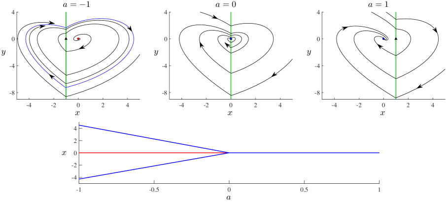
Figure 6.2: An illustration of HLB 4 for the valve generator model (6.19) with $h_{1}=0.6$ and $h_{2}=0.3$. By decreasing the value of $a$, a stable focus collides with the switching manifold $x=a$ when $a=0$ where it turns into an unstable focus and emits a stable limit cycle.

Theorem 6.2 is proved for piecewise-linear systems in Si18f and in general in Appendix B. As shown in Si18f , there can exist pseudo-equilibria but this only seems to occur over a relatively small fraction of parameter space.

The following equations model a valve generator (a simple electrical circuit):

$$\begin{split}\dot{x}&=y,\\ \dot{y}&=\begin{cases}-x-2h_{1}y,&x<a,\\ -x+2h_{2}y,&x>a.\end{cases}\end{split}$$ (6.19)

With $a=-1$ this is equation (8.5) of AnVi66 (a similar example is presented in Section 2.1 of MaLa12 ). The equations (6.19) are non-dimensionalised, where $x(t)$ represents voltage, and $h_{1}$ and $h_{2}$ are combinations of certain circuit parameters. In AnVi66 it is shown that (6.19) has a unique stable limit cycle when $a=-1$, $h_{1}>h_{2}$, and $0<h_{2}<1$. Here we allow $a$ to vary so that we can observe the limit cycle being created in an instance of HLB 4, see Fig. 6.2.

Assuming $0<h_{1}<1$ and $0<h_{2}<1$ (so that the equilibria are foci of opposite stability), (6.19) has a BEB in accordance with Theorem 6.2 when $a=0$. Here $\alpha=\frac{h_{2}}{\sqrt{1-h_{2}^{2}}}-\frac{h_{1}}{\sqrt{1-h_{1}^{2}}}$, thus $h_{1}>h_{2}$ implies $\alpha<0$ and hence a stable limit cycle. Also $\gamma=0$ because (6.19) has no sliding regions.

7 Slipping foci and folds in Filippov systems

In this section we suppose that each half-system of (6.1) has either a focus or an invisible fold on $x=0$ for all values of $\mu$ in a neighbourhood of $0$ (see already Fig. 7.1). So that a limit cycle may be created, we suppose that orbits near these points involve the same direction of rotation. We further suppose that these points ‘slip’ along $x=0$ as $\mu$ is varied and collide when $\mu=0$. There are three cases: both points are foci, HLB 5, one point is a focus and the other is a fold, HLB 6, and both points are folds, HLB 7. The third case (called ${\rm II}_{2}$ in KuRi03 ) is a generic codimension-one bifurcation for two-dimensional Filippov systems. It occurs, for instance, with on/off PD control of an inverted pendulum Ko17 (see §7.3), a similar automatic pilot model AnVi66 , and Welander’s ocean convection model Le16 .

In each case, a sliding region shrinks to a point (at $\mu=0$) and changes from attracting to repelling. The creation of a limit cycle in this fashion is called a pseudo-Hopf bifurcation in KuRi03 . Transversality and non-degeneracy conditions for these bifurcations were derived in CaLl17 for piecewise-linear systems. Here we generalise these results to allow nonlinear terms in $F_{L}$ and $F_{R}$. These terms only affect the qualitative behaviour of the bifurcation in the two-fold case. For analogous bifurcations involving visible folds, see KuRi03 ; TaLi12 .

7.1 The focus/focus case — HLB 5

Figure 7.1: A typical phase portrait of the Filippov system (6.1) subject to the assumptions of Theorem 7.1 with small $\mu>0$. The points $(0,\xi_{L})$ and $(0,\xi_{R})$ are boundary foci. The direction of sliding motion on $\Gamma$ is governed by the sign of $\gamma$, (7.6).

Figure 7.2: An illustration of HLB 5 for (7.7) with $\lambda_{L}=0.1$ and $\lambda_{R}=-0.5$. By increasing the value of $\mu$ two boundary foci collide causing an attracting sliding region to shrink to a point and reappear as a repelling sliding region and producing a stable limit cycle.

Here we suppose that for all values of $\mu$ in a neighbourhood of $0$, the left and right half-systems of (6.1) have equilibria at $(x,y)=(0,\xi_{L}(\mu))$ and $(x,y)=(0,\xi_{R}(\mu))$, respectively. That is,

$$f_{L}(0,\xi_{L}(\mu);\mu) =0, f_{R}(0,\xi_{R}(\mu);\mu) =0,$$ (7.1)

$$g_{L}(0,\xi_{L}(\mu);\mu) =0, g_{R}(0,\xi_{R}(\mu);\mu) =0,$$

for all sufficiently small $\mu\in\mathbb{R}$. We suppose that the equilibria coincide at the origin when $\mu=0$, that is

$$\xi_{L}(0)=\xi_{R}(0)=0.$$ (7.2)

We suppose $(0,\xi_{L}(\mu))$ is an unstable focus and $(0,\xi_{R}(\mu))$ is a stable focus, that is

$$\begin{split}{\rm eig}({\rm D}F_{L}(0,0;0))&=\lambda_{L}\pm{\rm i}\omega_{L}\,,\quad{\rm with~{}}\lambda_{L}>0,\omega_{L}>0,\\ {\rm eig}({\rm D}F_{R}(0,0;0))&=\lambda_{R}\pm{\rm i}\omega_{R}\,,\quad{\rm with~{}}\lambda_{R}<0,\omega_{R}>0,\end{split}$$ (7.3)

and that the foci have the same direction of rotation. To simplify the $\mu$-dependence we assume (without loss of generality) that both foci have clockwise rotation, Fig. 7.1. That is, $\frac{\partial f_{L}}{\partial y}(0,0;0)>0$ and $\frac{\partial f_{R}}{\partial y}(0,0;0)>0$. As with HLBs 1 and 4, the sign of

$$\alpha=\frac{\lambda_{L}}{\omega_{L}}+\frac{\lambda_{R}}{\omega_{R}},$$ (7.4)

governs the stability of the origin when $\mu=0$.

The distance between the foci is $|\beta\mu|+O\mathopen{}\mathclose{{}\left(\mu^{2}}\right)$, where

$$\beta=\mathopen{}\mathclose{{}\left(\frac{d\xi_{L}}{d\mu}-\frac{d\xi_{R}}{d\mu}\middle)}\right|_{\mu=0},$$ (7.5)

thus $\beta\neq 0$ is the transversality condition for HLB 5. Let $\Gamma\subset\mathbb{R}^{2}$ be the subset of the switching manifold bounded by the foci, see Fig. 7.1. Notice $\Gamma$ is a sliding region on which motion is governed by (3.7). With the above assumptions the numerator of (3.7) is $\gamma\mathopen{}\mathclose{{}\left(y-\xi_{L}(\mu)}\right)\mathopen{}\mathclose{{}\left(y-\xi_{R}(\mu)}\right)$, plus higher order terms, where

$$\gamma=\mathopen{}\mathclose{{}\left(\frac{\partial f_{L}}{\partial y}\frac{\partial g_{R}}{\partial y}-\frac{\partial f_{R}}{\partial y}\frac{\partial g_{L}}{\partial y}\middle)}\right|_{x=y=\mu=0}.$$ (7.6)

Theorem 7.1 (HLB 5).

Consider (6.1) where $F_{L}$ and $F_{R}$ are $C^{1}$. Suppose (7.1) and (7.2) are satisfied, where $\xi_{L}$ and $\xi_{R}$ are $C^{1}$. Suppose (7.3) is satisfied, $\frac{\partial f_{L}}{\partial y}(0,0;0)>0$, $\frac{\partial f_{R}}{\partial y}(0,0;0)>0$, and $\beta>0$. In a neighbourhood of $(x,y;\mu)=(0,0;0)$,

1. $\Gamma$ is an attracting sliding region for $\mu<0$ (and if $\gamma<0$ [$\gamma>0$] then $(0,\xi_{R}(\mu))$ [$(0,\xi_{L}(\mu))$] is stable while $(0,\xi_{L}(\mu))$ [$(0,\xi_{R}(\mu))$] is unstable) and a repelling sliding region for $\mu>0$,

2. if $\alpha<0$ [$\alpha>0$] there exists a unique stable [unstable] limit cycle for $\mu>0$ [$\mu<0$], and no limit cycle for $\mu<0$ [$\mu>0$].

The minimum and maximum $x$ and $y$-values of the limit cycle are asymptotically proportional to $|\mu|$, and the period limits to $\frac{\pi}{\omega_{L}}+\frac{\pi}{\omega_{R}}$ as $\mu\to 0$.

As an example consider

$$\begin{bmatrix}\dot{x}\\ \dot{y}\end{bmatrix}=\begin{cases}\begin{bmatrix}\lambda_{L}x+y\\ -x+\lambda_{L}y\end{bmatrix},&x<0,\\ \begin{bmatrix}\lambda_{R}x+y+\mu\\ -x+\lambda_{R}(y+\mu)\end{bmatrix},&x>0.\end{cases}$$ (7.7)

which satisfies the conditions of Theorem 7.1 when $\lambda_{L}>0$ and $\lambda_{R}<0$. Specifically we have $\xi_{L}(\mu)=0$ and $\xi_{R}(\mu)=-\mu$, thus $\beta=1$. Also $\alpha=\lambda_{L}+\lambda_{R}$ and $\gamma=\lambda_{R}-\lambda_{L}<0$. Fig. 7.2 shows a bifurcation diagram and representative phase portraits using values of $\lambda_{L}$ and $\lambda_{R}$ for which $\alpha<0$.

7.2 The focus/fold case — HLB 6

Figure 7.3: An illustration of HLB 6 for (7.14) with $\lambda_{L}=1$. By decreasing the value of $\mu$ a boundary focus and invisible fold collide causing an repelling sliding region to shrink to a point and reappear as an attracting sliding region and producing an unstable limit cycle.

Now suppose that for all values of $\mu$ in a neighbourhood of $0$ the left half-system has a focus at the origin. That is,

$$f_{L}(0,0;\mu) =0, g_{L}(0,0;\mu) =0,$$ (7.8)

and

$${\rm eig}({\rm D}F_{L}(0,0;0))=\lambda_{L}\pm{\rm i}\omega_{L}\,,\quad{\rm with~{}}\lambda_{L}\in\mathbb{R},\omega_{L}>0.$$ (7.9)

In order for the right half-system to have a fold at the origin when $\mu=0$ we suppose

$$f_{R}(0,0;0)=0.$$ (7.10)

As with HLB 5 we suppose $\frac{\partial f_{L}}{\partial y}(0,0;0)>0$ and $\frac{\partial f_{R}}{\partial y}(0,0;0)>0$ so that both half-systems involve clockwise rotation. Then $g_{R}(0,0;0)<0$ ensures the fold is invisible. Locally the right half-system has a unique fold at $(x,y)=(0,\zeta_{R}(\mu))$, where

$$\frac{d\zeta_{R}}{d\mu}(0)=-\frac{\frac{\partial f_{R}}{\partial\mu}(0,0;0)}{\frac{\partial f_{R}}{\partial y}(0,0;0)}.$$ (7.11)

It follows that the transversality condition for HLB 6 is $\beta\neq 0$, where

$$\beta=\frac{\partial f_{R}}{\partial\mu}(0,0;0).$$ (7.12)

Let $\Gamma\subset\mathbb{R}^{2}$ be the subset of the switching manifold bounded by the focus $(0,0)$ and the fold $(0,\zeta_{R}(\mu))$. When $\mu=0$ the stability of the origin is governed by the sign of

$$\alpha=\lambda_{L}\,,$$ (7.13)

as can be seen by composing the return maps (4.7) and (4.14).

Theorem 7.2 (HLB 6).

Consider (6.1) where $F_{L}$ and $F_{R}$ are $C^{1}$. Suppose (7.8), (7.9), and (7.10) are satisfied, $\frac{\partial f_{L}}{\partial y}(0,0;0)>0$, $\frac{\partial f_{R}}{\partial y}(0,0;0)>0$, $g_{R}(0,0;0)<0$, and $\beta>0$. In a neighbourhood of $(x,y;\mu)=(0,0;0)$,

1. the origin is the unique stationary solution and is stable for $\mu<0$ and unstable for $\mu>0$ ($\Gamma$ is an attracting sliding region for $\mu<0$ and a repelling sliding region for $\mu>0$),

2. if $\alpha<0$ [$\alpha>0$] there exists a unique stable [unstable] limit cycle for $\mu>0$ [$\mu<0$], and no limit cycle for $\mu<0$ [$\mu>0$].

The maximum $x$-value of limit cycle is asymptotically proportional to $\mu^{2}$, the minimum $x$-value and minimum and maximum $y$-values of the limit cycle are asymptotically proportional to $|\mu|$, and the period limits to $\frac{\pi}{\omega_{L}}$ as $\mu\to 0$.

As a minimal example consider

$$\begin{bmatrix}\dot{x}\\ \dot{y}\end{bmatrix}=\begin{cases}\begin{bmatrix}\lambda_{L}x+y\\ -x+\lambda_{L}y\end{bmatrix},&x<0,\\ \begin{bmatrix}y+\mu\\ -1\end{bmatrix},&x>0,\end{cases}$$ (7.14)

which satisfies the conditions of Theorem 7.2. Fig. 7.3 shows representative phase portraits and a bifurcation diagram using $\lambda_{L}=1$ (here $\alpha>0$ so an unstable limit cycle is created).

7.3 The two-fold case — HLB 7

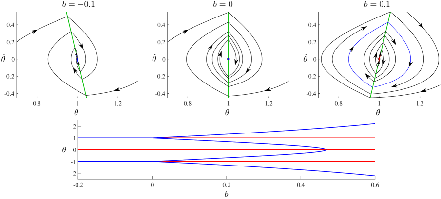
Figure 7.4: Phase portraits and a bifurcation diagram of the controlled pendulum model (7.19) with (7.20). The system is symmetric and exhibits two instances of HLB 7 at $b=0$. For each instance, by increasing the value of $b$ two invisible folds collide causing an attracting sliding region to shrink to a point and reappear as a repelling sliding region and producing a stable limit cycle.

Here we suppose both half systems of (6.1) have a clockwise-rotating invisible fold at the origin when $\mu=0$. That is,

$$f_{L}(0,0;0)=f_{R}(0,0;0)=0,$$ (7.15)

and $\frac{\partial f_{L}}{\partial y}(0,0;0)>0$, $\frac{\partial f_{R}}{\partial y}(0,0;0)>0$, $g_{L}(0,0;0)>0$ and $g_{R}(0,0;0)<0$. The folds persist for small $\mu\neq 0$ and the distance between them is $|\beta\mu|+O\mathopen{}\mathclose{{}\left(\mu^{2}}\right)$, where

$$\beta=\mathopen{}\mathclose{{}\left(\frac{\frac{\partial f_{R}}{\partial\mu}}{\frac{\partial f_{R}}{\partial y}}-\frac{\frac{\partial f_{L}}{\partial\mu}}{\frac{\partial f_{L}}{\partial y}}}\right)\bigg{|}_{x=y=\mu=0}.$$ (7.16)

Let $\Gamma$ be the subset of $x=0$ bounded by the two folds. Also let

$$\alpha=\mathopen{}\mathclose{{}\left(\sigma_{{\rm fold},L}-\sigma_{{\rm fold},R}\middle)}\right|_{\mu=0}\,,$$ (7.17)

where (4.12) is evaluated for both left and right half-systems as indicated in (7.17) with subscripts.

Theorem 7.3 (HLB 7).

Consider (6.1) where $F_{L}$ and $F_{R}$ are $C^{2}$. Suppose (7.15) is satisfied, $\frac{\partial f_{L}}{\partial y}(0,0;0)>0$, $\frac{\partial f_{R}}{\partial y}(0,0;0)>0$, $g_{L}(0,0;0)>0$, $g_{R}(0,0;0)<0$, and $\beta>0$. In a neighbourhood of $(x,y;\mu)=(0,0;0)$,

1. there exists a unique stationary solution: a pseudo-equilibrium in $\Gamma$ that is stable for $\mu<0$ and unstable for $\mu>0$ ($\Gamma$ is an attracting sliding region for $\mu<0$ and a repelling sliding region for $\mu>0$),

2. if $\alpha<0$ [$\alpha>0$] there exists a unique stable [unstable] limit cycle for $\mu>0$ [$\mu<0$], and no limit cycle for $\mu<0$ [$\mu>0$].

The minimum and maximum $x$-values of the limit cycle are asymptotically proportional to $|\mu|$, and the minimum and maximum $y$-values of the limit cycle are asymptotically proportional to $\sqrt{|\mu|}$, and its period is

$$T=\mathopen{}\mathclose{{}\left(\frac{2}{g_{L}(0,0;0)}-\frac{2}{g_{R}(0,0;0)}}\right)\sqrt{\frac{-3\beta\mu}{\alpha}}+o\mathopen{}\mathclose{{}\left(\sqrt{\mu}}\right).$$ (7.18)

To illustrate HLB 7 we consider an inverted pendulum subject to on/off control. There have been many studies of inverted pendulums with a control law that seeks to maintain the pendulum in a roughly vertical position, with applications to robotics BaMi10 and human postural sway MiCa09 . On/off control strategies are popular as they are simple, easy to implement, and can be highly effective AsTa09 ; MiTo09 ; StIn06 . Typically the time lag between when the controller makes measurements and is able to implement control is an important factor, but this is not considered here, see §10.

Specifically we consider the model studied in Ko17 :

$$\ddot{\theta}=\begin{cases}a\theta,&|\theta-b\dot{\theta}|<\theta^{*},\\ (a-K_{p})\theta-K_{d}\dot{\theta},&|\theta-b\dot{\theta}|>\theta^{*}.\end{cases}$$ (7.19)

Here $\theta(t)$ represents the angular displacement of the pendulum from vertical. In the absence of control, $\theta(t)$ is assumed to vary according to $\ddot{\theta}=a\theta$ for some constant $a>0$ (a reasonable assumption for small angles). The applied control force is a linear combination of $\theta$ and $\dot{\theta}$ (PD control). With $b=0$, the control is applied when $|\theta|$ exceeds a threshold angle $\theta^{*}$, and $b\neq 0$ incorporates dependency on $\dot{\theta}$.

Fig. 7.4 shows the dynamics near the switching manifold $\theta=\theta^{*}+b\dot{\theta}$ using parameter values given in Ko17 :

$$a =0.5, K_{p} =1, K_{d} =1, \theta^{*} =1.$$ (7.20)

Two invisible folds collide at $(\theta,\dot{\theta})=(\theta^{*},0)$ when $b=0$, and a stable limit cycle exists for $b>0$. The system is symmetric and exhibits the same dynamics near the other switching manifold $\theta=-\theta^{*}+b\dot{\theta}$. Thus two stable limit cycles are created at $b=0$ in symmetric instances of HLB 7. At $b\approx 0.47$ the limit cycles become homoclinic to the origin and merge into a single symmetric limit cycle.

Theorem 7.18 can be applied to this system via the coordinate change

$$\begin{split}x&=\theta-(\theta^{*}+b\dot{\theta}),\\ y&=\dot{\theta}.\end{split}$$

It is a simple exercise to show that, with the parameter values (7.20), the conditions of Theorem 7.18 are met with $\alpha=\frac{-K_{p}}{(K_{p}-a)\theta^{*}}<0$, hence a stable limit cycle is created as described above.

8 Fixed foci and folds in Filippov systems

In this section we suppose that each half-system of (6.1) has either a focus or an invisible fold at the origin for all values of $\mu$ in a neighbourhood of $0$. We also suppose the direction of rotation is the same on both sides. With these assumptions no sliding motion occurs locally. The origin is a stationary solution and we suppose its stability changes at $\mu=0$. Generically a limit cycle is created and, as in the previous section, there are three cases: (i) focus/focus, HLB 8, (ii) focus/fold, HLB 9, (iii) two-fold, HLB 10.

The focus/focus case occurs in a simple braking model for a car or bike and called a generalised Hopf bifurcation in KuMo01 ; ZoKu06 , see also ChZo10 ; LlPo08 . For physical reasons the nonlinear terms in this model are cubic; consequently the amplitude of the limit cycle is asymptotically proportional to $\sqrt{|\mu|}$. The absence of quadratic terms is a degeneracy in the context of general Filippov systems. Below we show that non-degenerate quadratic terms produce asymptotically linear growth for the amplitude. For the more general situation that switching manifolds emanate from the origin at arbitrary angles and the origin is a focus in each region bounded by these manifolds, see AkKa17 ; AkAr09 ; ZoKu05 .

The two-fold case was described briefly by Filippov (see page 238 of Fi88 ), is analysed for piecewise-quadratic systems in LiHu14 , and occurs for a buck converter (a type of DC/DC power converter) with idealised switching FrPo12 , although here the model lacks nonlinear terms necessary for a limit cycle.

To analyse the HLB in each case we use a Poincaré map: given $r>0$ let $P(r)$ denote the $y$-value at which the forward orbit of $(x,y)=(0,r)$ next intersects the positive $y$-axis. If there exists $n\geq 1$ such that

$$P(r)=r+V_{n}r^{n}+O\mathopen{}\mathclose{{}\left(r^{n+1}}\right),$$

where $V_{n}\neq 0$, then $V_{n}$ is called the $n^{\rm th}$ Lyapunov constant Ku00 . For the three scenarios considered here, the bifurcation occurs when $V_{n}=0$ (with $n=1$ for the focus/focus and focus/fold cases, and $n=2$ for the two-fold case). The criticality of the bifurcation is determined by the sign of the next generically non-zero Lyapunov exponent $V_{m}$ (with $m=2$ for the focus/focus and focus/fold cases, and $m=4$ for the two-fold case). For the focus/focus and focus/fold cases, Lyapunov constants were obtained in CoGa01 by using differential equations with a single complex variable. Higher order scenarios are described in GaTo03 ; LiHa09 (for the focus/focus case) and in LiHa12 (for the focus/fold and two-fold cases); see also YaHa11 for piecewise-Hamiltonian systems.

8.1 The focus/focus case — HLB 8

Here we suppose

$$f_{L}(0,0;\mu) =0, f_{R}(0,0;\mu) =0,$$ (8.1)

$$g_{L}(0,0;\mu) =0, g_{R}(0,0;\mu) =0,$$

for all values of $\mu$ in a neighbourhood of $0$, and

$$\begin{split}{\rm eig}({\rm D}F_{L}(0,0;\mu))&=\lambda_{L}(\mu)\pm{\rm i}\omega_{L}(\mu),\\ &\quad~{}{\rm with~{}}\lambda_{L}(\mu)>0,\omega_{L}(\mu)>0,\\ {\rm eig}({\rm D}F_{R}(0,0;\mu))&=\lambda_{R}(\mu)\pm{\rm i}\omega_{R}(\mu),\\ &\quad~{}{\rm with~{}}\lambda_{R}(\mu)<0,\omega_{R}(\mu)>0.\end{split}$$ (8.2)

Suppose the two foci involve the same direction of rotation and let $P(r;\mu)$ denote the $y$-value of the next intersection of the forward orbit of $(x,y)=(0,r)$ with the positive $y$-axis. By applying Lemma 4.4 to both left and right half-systems, we obtain $P(r;\mu)={\rm e}^{\Lambda(\mu)\pi}r+O\mathopen{}\mathclose{{}\left(r^{2}}\right)$, where

$$\Lambda(\mu)=\frac{\lambda_{L}(\mu)}{\omega_{L}(\mu)}+\frac{\lambda_{R}(\mu)}{\omega_{R}(\mu)}.$$ (8.3)

Thus the stability of the origin is determined by the sign of $\Lambda$. For HLB 8 we suppose $\Lambda(0)=0$ and $\beta\neq 0$ where

$$\beta=\frac{d\Lambda}{d\mu}(0).$$ (8.4)

The $r^{2}$-term in $P(r;0)$ governs the criticality of the bifurcation. In Appendix D we show that

$$\alpha=\mathopen{}\mathclose{{}\left(\chi_{{\rm focus},L}-\chi_{{\rm focus},R}\middle)}\right|_{\mu=0}\,,$$ (8.5)

is a factor in the coefficient of the $r^{2}$-term, where (4.5) is evaluated for both left and right half-systems as indicated with subscripts.

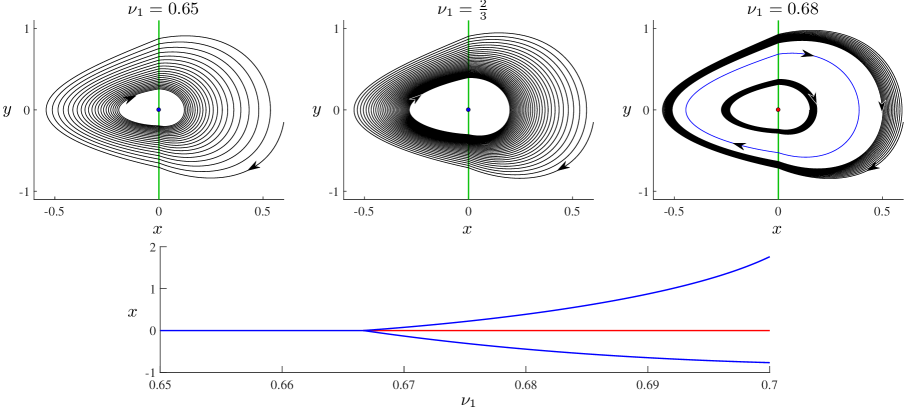
Figure 8.1: An illustration of HLB 8 for the bilinear oscillator (8.7) with (8.10), $b=0.5$, $\nu_{2}=1$, and $\hat{x}=0$. By increasing the value of $\nu_{1}$ the origin (a ‘merged focus’) loses stability when $\nu_{1}=\frac{4b}{3}$ and emits a stable limit cycle.

Theorem 8.1 (HLB 8).

Consider (6.1) where $F_{L}$ and $F_{R}$ are $C^{2}$. Suppose (8.1) and (8.2) are satisfied, $\frac{\partial f_{L}}{\partial y}(0,0;0)\frac{\partial f_{R}}{\partial y}(0,0;0)>0$, $\Lambda(0)=0$, and $\beta>0$. In a neighbourhood of $(x,y;\mu)=(0,0;0)$,

1. the origin is the unique stationary solution and is stable for $\mu<0$ and unstable for $\mu>0$,

2. if $\alpha<0$ [$\alpha>0$] there exists a unique stable [unstable] limit cycle for $\mu>0$ [$\mu<0$], and no limit cycle for $\mu<0$ [$\mu>0$].

The minimum and maximum $x$ and $y$-values of the limit cycle are asymptotically proportional to $|\mu|$, and its period is

$$T=\frac{\pi}{\omega_{L}(0)}+\frac{\pi}{\omega_{R}(0)}+O(\mu).$$ (8.6)

As an example consider the bilinear oscillator:

$$\begin{split}\dot{x}&=y,\\ \dot{y}&=\begin{cases}-k_{L}x-b_{L}y+F_{\rm apply}(y),&x<0,\\ -k_{L}x-k_{R}(x+\hat{x})-(b_{L}+b_{R})y+F_{\rm apply}(y),&x>0.\end{cases}\end{split}$$ (8.7)

where

$$F_{\rm apply}(y)=\nu_{1}y+\nu_{2}y^{2},$$ (8.8)

represents an applied force. The variables $x(t)$ and $y(t)$ can be interpreted as the position and velocity of an oscillator that undergoes compliant impacts at $x=0$. All parameters in (8.7) are non-negative constants (in particular $\hat{x}>0$ is a prestress distance, see SiHo13 ). This model is motivated by experimental studies, particularly InPa08b ; MaIn08 , but the parameter values used here are purely chosen to illustrate the HLBs. For other studies of bilinear oscillators refer to DiBu08 ; PaYa08 ; ShHo83b .

With $\hat{x}=0$ the origin is an equilibrium of both half-systems. By writing the associated eigenvalues in the form (8.2) we obtain

$$\lambda_{L} =\frac{\nu_{1}-b_{L}}{2},$$ (8.9)

$$\lambda_{R} =\frac{\nu_{1}-b_{L}-b_{R}}{2},$$

$$\omega_{L} =\sqrt{k_{L}-\frac{(\nu_{1}-b_{L})^{2}}{4}},$$

$$\omega_{R} =\sqrt{k_{L}+k_{R}-\frac{(\nu_{1}-b_{L}-b_{R})^{2}}{4}}.$$

Let us fix

$$k_{L} =1, k_{R} =3,$$ (8.10)

$$b_{L} =b, b_{R} =b,$$

for some $b>0$. Then $\Lambda$ is zero when $\nu_{1}=\frac{4b}{3}$, thus to apply Theorem 8.6 we define $\mu=\nu_{1}-\frac{4b}{3}$. This gives $\beta=\frac{d\Lambda}{d\nu_{1}}\big{|}_{\nu_{1}=\frac{4b}{3}}=\frac{162}{\mathopen{}\mathclose{{}\left(36-b^{2}}\right)^{\frac{3}{2}}}$ and $\alpha=\frac{-9b\nu_{2}}{2\mathopen{}\mathclose{{}\left(81-2b^{2}}\right)}$.

Fig. 8.1 shows a bifurcation diagram using $b=0.5$ and $\nu_{2}=1$. Since $\beta>0$ and $\alpha<0$, a stable limit cycle is created at $\nu_{1}=\frac{4b}{3}$. The limit cycle grows quite quickly because $|\alpha|$ is relatively small ($\alpha\approx-0.0280$) and the amplitude of the limit cycle is inversely proportional to $|\alpha|$, see (D.2). For the same reason the rate at which orbits converge to the limit cycle is relatively slow.

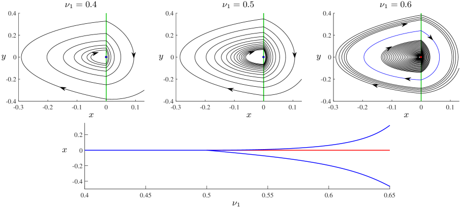
Figure 8.2: An illustration of HLB 9 for the bilinear oscillator (8.7) with (8.10), $b=0.5$, $\nu_{2}=1$, and $\hat{x}=0.1$. By increasing the value of $\nu_{1}$ the origin (a focus for the left half-system and an invisible fold for the right half-system) loses stability when $\nu_{1}=b$ and emits a limit cycle. The limit cycle is stable because $\alpha=\frac{-b_{R}}{3k_{R}\hat{x}}=-\frac{5}{9}<0$.

8.2 The focus/fold case — HLB 9

Here we suppose the left half-system has a focus at the origin, i.e.

$$f_{L}(0,0;\mu) =0, g_{L}(0,0;\mu) =0,$$ (8.11)

and

$$\begin{split}{\rm eig}({\rm D}F_{L}(0,0;\mu))&=\lambda_{L}(\mu)\pm{\rm i}\omega_{L}(\mu),\\ &\quad~{}{\rm with~{}}\lambda_{L}(\mu)\in\mathbb{R},\omega_{L}(\mu)>0,\end{split}$$ (8.12)

for all values of $\mu$ in a neighbourhood of $0$. We suppose the right half-system has an invisible fold at the origin, thus

$$f_{R}(0,0;\mu)=0,$$ (8.13)

and $\gamma<0$ where

$$\gamma=\mathopen{}\mathclose{{}\left(\frac{\partial f_{R}}{\partial y}\,g_{R}\middle)}\right|_{x=y=\mu=0}.$$ (8.14)

Also suppose both half-systems involve the same direction of rotation.

In this situation the stability of the origin is simply determined by the sign of $\lambda_{L}(\mu)$. Thus for HLB 9 we assume $\lambda_{L}(0)=0$ and let

$$\beta=\frac{d\lambda_{L}}{d\mu}(0).$$ (8.15)

As shown below the criticality of the bifurcation is determined by the sign of

$$\alpha=\mathopen{}\mathclose{{}\left(\chi_{{\rm focus},L}-\frac{\sigma_{{\rm fold},R}}{3}\middle)}\right|_{\mu=0},$$ (8.16)

where (4.5) is evaluated for the left half-system and (4.12) is evaluated for the right half-system.

Theorem 8.2 (HLB 9).

Consider (6.1) where $F_{L}$ and $F_{R}$ are $C^{2}$. Suppose (8.11), (8.12), and (8.13) are satisfied, $\frac{\partial f_{L}}{\partial y}(0,0;0)\frac{\partial f_{R}}{\partial y}(0,0;0)>0$, $\lambda_{L}(0)=0$, $\beta>0$, and $\gamma<0$. In a neighbourhood of $(x,y;\mu)=(0,0;0)$,

1. the origin is the unique stationary solution and is stable for $\mu<0$ and unstable for $\mu>0$,

2. if $\alpha<0$ [$\alpha>0$] there exists a unique stable [unstable] limit cycle for $\mu>0$ [$\mu<0$], and no limit cycle for $\mu<0$ [$\mu>0$].

The maximum $x$-value of the limit cycle is asymptotically proportional to $\mu^{2}$, its minimum $x$-value and minimum and maximum $y$-values are asymptotically proportional to $|\mu|$, and its period is

$$T=\frac{\pi}{\omega_{L}(0)}+O(\mu).$$ (8.17)

To illustrate Theorem (8.17) we consider (8.7) with $\hat{x}>0$. Again $\lambda_{L}$ and $\omega_{L}$ are given by (8.9). The bifurcation occurs when $\lambda_{L}=0$, thus here we use $\mu=\nu_{1}-b_{L}$ for which $\beta=\frac{1}{2}$.

To evaluate $\alpha$ we first observe that the $\ell_{3}\frac{\partial^{2}g_{L}}{\partial y^{2}}$-term is only potential contribution to $\chi_{{\rm focus},L}$, see (4.5), but $\ell_{3}=\frac{k_{L}(\nu_{1}-b_{L})}{2}$ is zero at the bifurcation hence $\chi_{{\rm focus},L}=0$. From (4.12) we obtain $\sigma_{{\rm fold},R}=\frac{\nu_{1}-b_{L}-b_{R}}{-k_{R}\hat{x}}$ and so $\alpha=\frac{-b_{R}}{3k_{R}\hat{x}}$. Fig. 8.2 illustrates the dynamics near the bifurcation with typical parameter values.

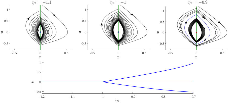
Figure 8.3: An illustration of HLB 10 for (8.24) with $\eta_{1}=1$. By increasing the value of $\eta_{2}$, the origin (an invisible-invisible two-fold) loses stability when $\nu_{2}=-1$ and emits a stable limit cycle. Take care to note that the bifurcation diagram only shows the asymptotically linear growth of the minimum and maximum $x$-values of the limit cycle; the amplitude (or diameter) of the limit cycle is asymptotically proportional to $\sqrt{\eta_{2}+1}$ (see Theorem 8.23).

8.3 The two-fold case — HLB 10

We now suppose that for all values of $\mu$ in a neighbourhood of $0$, the origin is an invisible fold for both half-systems of (6.1). Thus

$$f_{L}(0,0;\mu) =0, f_{R}(0,0;\mu) =0,$$ (8.18)

and $\gamma_{L}>0$ and $\gamma_{R}<0$ where

$$\gamma_{J}=\mathopen{}\mathclose{{}\left(\frac{\partial f_{J}}{\partial y}\,g_{J}\middle)}\right|_{x=y=\mu=0},$$ (8.19)

for each $J\in\{L,R\}$. Again suppose both half-systems involve the same direction of rotation.

Let $\sigma_{{\rm fold},J}(\mu)$ and $\chi_{{\rm fold},J}(\mu)$ be the result of evaluating (4.12) and (4.13) with the vector field $F=F_{J}$. As shown in Appendix D, the stability of the origin is governed by the sign of

$$\Lambda(\mu)=\sigma_{{\rm fold},L}(\mu)-\sigma_{{\rm fold},R}(\mu).$$ (8.20)

Thus for HLB 10 we assume $\Lambda(0)=0$ and let

$$\beta=\frac{d\Lambda}{d\mu}(0).$$ (8.21)

We also let

$$\alpha=\chi_{{\rm fold},L}(0)-\chi_{{\rm fold},R}(0).$$ (8.22)

Theorem 8.3 (HLB 10).

Consider (6.1) where $F_{L}$ and $F_{R}$ are $C^{4}$. Suppose (8.18) is satisfied, $\frac{\partial f_{L}}{\partial y}(0,0;0)\frac{\partial f_{R}}{\partial y}(0,0;0)>0$, $\Lambda(0)=0$, $\beta>0$, $\gamma_{L}>0$, and $\gamma_{R}<0$. In a neighbourhood of $(x,y;\mu)=(0,0;0)$,

1. the origin is the unique stationary solution and is stable for $\mu<0$ and unstable for $\mu>0$,

2. if $\alpha<0$ [$\alpha>0$] there exists a unique stable [unstable] limit cycle for $\mu>0$ [$\mu<0$], and no limit cycle for $\mu<0$ [$\mu>0$].

The minimum and maximum $x$-values of the limit cycle are asymptotically proportional to $|\mu|$, and the minimum and maximum $y$-values of the limit cycle are asymptotically proportional to $\sqrt{|\mu|}$, and the period is

$$T=\mathopen{}\mathclose{{}\left(\frac{2}{g_{L}(0,0;0)}-\frac{2}{g_{R}(0,0;0)}}\right)\sqrt{\frac{-5\beta\mu}{\alpha}}+o\mathopen{}\mathclose{{}\left(\sqrt{|\mu|}}\right).$$ (8.23)

As an abstract example consider

$$\begin{bmatrix}\dot{x}\\ \dot{y}\end{bmatrix}=\begin{cases}\begin{bmatrix}x+y\\ 1\end{bmatrix},&x<0,\\ \begin{bmatrix}y\\ -1+\eta_{1}x+\eta_{2}y\end{bmatrix},&x>0,\end{cases}$$ (8.24)

where $\eta_{1},\eta_{2}\in\mathbb{R}$ are parameters. Here $\sigma_{{\rm fold},L}=1$ and $\sigma_{{\rm fold},R}=-\eta_{2}$, so in Theorem 8.23 we use $\mu=\eta_{2}+1$, for which $\beta=1$. Also $\chi_{{\rm fold},L}=\frac{22}{9}$ and $\chi_{{\rm fold},R}=\frac{22}{9}+\eta_{1}$, thus $\alpha=-\eta_{1}$. Fig. 8.3 shows phase portraits and a bifurcation diagram using $\eta_{1}=1$.

9 Hybrid systems

State variables of hybrid systems experience jumps between periods of continuous evolution. The continuous evolution is governed by differential equations, the jumps are defined by maps, and the maps are applied when certain time-dependent or state-dependent conditions are met. Hybrid systems naturally model mechanical systems with hard impacts, ecological systems with periodic culling or addition of population, and many control systems. A smooth dynamical system becomes hybrid when it is combined with control law that gives an occasional kick to the state of the system. Such control laws are often both highly effective and efficient ChEl05 .

Hybrid systems are broad and this is reflected in the theory that has been developed for them HaCh06 ; LeNi10 ; Pl10 ; VaSc00 . Limit cycles involving jumps are often large amplitude, and multi-jump limit cycles are often best analysed via graph-theoretic techniques MaSa00 . This paper concerns small-amplitude limit cycles for which a local analysis is appropriate.

In §9.1 we study BEBs in hybrid systems involving a single map that leaves one variable unchanged. Such systems arise when impacts are modelled as instantaneous events (velocity is reversed but position is unchanged). In §9.2 we study hybrid systems with a single map (most naturally interpreted as an impulse) where the domain and range of the map intersect at a regular equilibrium. Proofs are provided in Appendices E and F.

9.1 Impacting systems — HLBs 11–13

Here we study systems of the form

$$\begin{split}\begin{bmatrix}\dot{x}\\ \dot{y}\end{bmatrix}&=F(x,y;\mu),{\rm~{}for~{}}x<0,\\ y&\mapsto\phi(y;\mu),{\rm~{}when~{}}x=0,\end{split}$$ (9.1)

and write

$$F(x,y;\mu)=\begin{bmatrix}f(x,y;\mu)\\ g(x,y;\mu)\end{bmatrix},$$

where $f$, $g$, and $\phi$ are smooth functions. Orbits evolve in $\Omega_{L}=\mathopen{}\mathclose{{}\left\{(x,y)\,\middle|\,x<0,y\in\mathbb{R}}\right\}$ following the vector field $F$ until reaching $x=0$ at which time the map $\phi$ is applied. The variables $x(t)$ and $y(t)$ may be interpreted as the position and velocity of an object that undergoes instantaneous impacts at $x=0$, where $\phi$ is the impact law. Define

$${\rm sgn}(a)=\begin{cases}-1,&a<0,\\ 0,&a=0,\\ 1,&a>0.\end{cases}$$ (9.2)

We assume

$${\rm sgn}\mathopen{}\mathclose{{}\left(f(0,y;\mu)}\right)={\rm sgn}(y),\quad\text{for all}~{}y,\mu\in\mathbb{R},$$ (9.3)

so that orbits following $F$ depart the negative $y$-axis and arrive at the positive $y$-axis, see Fig. 9.1. We also assume

$${\rm sgn}\mathopen{}\mathclose{{}\left(\phi(y;\mu)}\right)=-{\rm sgn}(y),\quad\text{for all}~{}y\geq 0,\,\text{and all}~{}\mu\in\mathbb{R}.$$ (9.4)

This ensures that for any positive impact velocity $y$, the rebound velocity $\phi(y;\mu)$ is negative and that impacts impart no change when $y=0$.

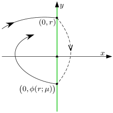
Figure 9.1: Part of a typical orbit of the impacting system (9.1).

The system (9.1) experiences a BEB when a regular equilibrium collides with $x=0$. At the bifurcation the equilibrium is necessarily located at $(x,y)=(0,0)$ by (9.3). As detailed in Section 5.1.3 of DiNo08 , there are four generic topologically distinct scenarios in which a local limit cycle is created in this type of BEB. If the equilibrium is a focus, a limit cycle may exist when the equilibrium is admissible (HLB 11) or when the equilibrium is virtual (HLB 12). If the equilibrium is a node, a limit cycle may exist when the node is virtual (HLB 13). If the equilibrium is a saddle, a limit cycle may be created but the BEB is of nonsmooth-fold type (thus here it is not treated as Hopf-like). As with HLBs 1–4, in generic situations the local dynamics are determined by linear terms MaWa18 .

In DiNo08 this class of BEBs is analysed by introducing a flow in $x>0$ that simulates the action of the map $\phi$ and then applying known results for piecewise-smooth continuous systems (such as Theorems 5.1–5.2). This approach involves little work although corrections are needed near $x=0$ because the vector field cannot be made to be continuous here for all values of $\mu$. The theorems presented below are instead proved by directly analysing a Poincaré map because the computationally intensive calculations are already covered by Lemma 4.6.

We suppose the BEB occurs when $\mu=0$, thus

$$g(0,0;0)=0.$$ (9.5)

Notice $f(0,0;0)=0$ is already implied by (9.3). If the Jacobian matrix ${\rm D}F(0,0;0)$ is invertible then, locally, (9.1) has a unique regular equilibrium with an $x$-value of $\frac{-\beta\mu}{\det\mathopen{}\mathclose{{}\left({\rm D}F(0,0;0)}\right)}+o(\mu)$, where

$$\beta=-\mathopen{}\mathclose{{}\left(\frac{\partial g}{\partial\mu}\frac{\partial f}{\partial y}\middle)}\right|_{x=y=\mu=0}.$$ (9.6)

Folds, sliding motion, and pseudo-equilibria defined above for Filippov systems admit analogous definitions for impacting systems. For details the reader is referred to DiBu08 ; DiNo08 . Since $f(0,0;\mu)=0$ by (9.3), if $g(0,0;\mu)\neq 0$ then the origin is a visible fold if $\beta\mu>0$ and an invisible fold if $\beta\mu<0$ (compare Definition 3.3). If the fold is visible, the orbit through the fold simply follows the tangent trajectory. If the fold is invisible, it is a stationary solution that may be viewed as a pseudo-equilibrium. If it is stable nearby orbits typically arrive at the pseudo-equilibrium in finite time via an infinite sequence of impacts — this is the Zeno phenomenon JoEg99 ; ZhJo01 . If it is unstable this occurs in backwards time NoDa11 .

The following lemma (proved in Appendix E) clarifies the existence and stability of the regular equilibrium and the pseudo-equilibrium (which is the origin when $\beta\mu<0$). Here we assume $\det({\rm D}F(0,0;0))>0$ so that these equilibria are admissible on different sides of the BEB (i.e. the bifurcation corresponds to persistence not a nonsmooth-fold). This assumption also implies that the regular equilibrium is not a saddle. Also we let

$$\gamma=-\frac{\partial\phi}{\partial y}(0;0),$$ (9.7)

and notice $\gamma\geq 0$ by (9.4).

Lemma 9.1.

Consider (9.1) where $F$ and $\phi$ are $C^{1}$. Suppose (9.3), (9.4), and (9.5) are satisfied, $\beta>0$, and $\det({\rm D}F(0,0;0))>0$. Let $\lambda=\frac{1}{2}\,{\rm trace}({\rm D}F(0,0;0))$. In a neighbourhood of $(x,y;\mu)=(0,0;0)$ there exists a unique stationary solution:

1. a stable [unstable] regular equilibrium in $\Omega_{L}$ if $\lambda<0$ [$\lambda>0$] for $\mu>0$,

2. and a stable [unstable] pseudo-equilibrium if $\gamma<1$ [$\gamma>1$] at the origin for $\mu<0$.

Now suppose

$${\rm eig}({\rm D}F(0,0;0))=\lambda\pm{\rm i}\omega,\quad{\rm with~{}}\lambda\in\mathbb{R},\omega>0,$$ (9.8)

so that the regular equilibrium is a focus. Consider the forward orbit of a point $(0,r)$, with $r>0$, when $\mu=0$. This point is mapped to $\mathopen{}\mathclose{{}\left(0,-\gamma r+o(r)}\right)$, then revolves to $\mathopen{}\mathclose{{}\left(0,\gamma{\rm e}^{\frac{\lambda\pi}{\omega}}r+o(r)}\right)$ by Lemma 4.4. For this reason the sign of

$$\alpha=\ln(\gamma)+\frac{\lambda\pi}{\omega},$$ (9.9)

determines the stability of the origin when $\mu=0$ (assuming $\gamma>0$).

In order for a limit cycle to be created at $\mu=0$ there needs to be competing actions of attraction and repulsion. Specifically we require $\lambda\ln(\gamma)<0$ so that (by Lemma 9.1) the regular equilibrium and pseudo-equilibrium are of opposite stability. There are two cases: If $\lambda\alpha<0$ then the stability of the regular equilibrium differs from the stability of the origin when $\mu=0$ (HLB 11). Here a limit cycle exists when the regular equilibrium is admissible. Notice the limit cycle completes more than half a revolution about the equilibrium so its period $T$ satisfies $\frac{\pi}{\omega}<T<\frac{2\pi}{\omega}$. If $\lambda\alpha>0$ then the stability of the regular equilibrium is the same as the stability of the origin when $\mu=0$ (HLB 12). Here a limit cycle exists when the regular equilibrium is virtual (and so $0<T<\frac{\pi}{\omega}$). In both cases the stability of the limit cycle is the same as the stability of the origin when $\mu=0$.

Theorem 9.2 (HLB 11).

Consider (9.1) where $F$ and $\phi$ are $C^{2}$. Suppose (9.3), (9.4), (9.5), (9.8) are satisfied, $\beta>0$, $\lambda\ln(\gamma)<0$, and $\lambda\alpha<0$. In a neighbourhood of $(x,y;\mu)=(0,0;0)$, if $\alpha<0$ [$\alpha>0$] then there exists a unique stable [unstable] limit cycle for $\mu>0$, and no limit cycle for $\mu<0$. The minimum $x$-value and the minimum and maximum $y$-values of the limit cycle are asymptotically proportional to $\mu$, and its period is $T=T_{0}+O(\mu)$, where $T_{0}$ satisfies

$$\gamma{\rm e}^{2\lambda T_{0}}=\frac{\varrho\mathopen{}\mathclose{{}\left(\omega T_{0};\frac{\lambda}{\omega}}\right)}{\varrho\mathopen{}\mathclose{{}\left(\omega T_{0};-\frac{\lambda}{\omega}}\right)},$$ (9.10)

and $\varrho$ is defined by (4.22).

Theorem 9.3 (HLB 12).

Consider (9.1) where $F$ and $\phi$ are $C^{2}$. Suppose (9.3), (9.4), (9.5), (9.8) are satisfied, $\beta>0$, $\lambda\ln(\gamma)<0$, and $\lambda\alpha>0$. In a neighbourhood of $(x,y;\mu)=(0,0;0)$, if $\alpha<0$ [$\alpha>0$] then there exists a unique stable [unstable] limit cycle for $\mu<0$, and no limit cycle for $\mu>0$. The minimum $x$-value and the minimum and maximum $y$-values of the limit cycle are asymptotically proportional to $\mu$, and its period is $T=T_{0}+O(\mu)$, where $T_{0}$ satisfies (9.10).

Now suppose the regular equilibrium is a node and write

$${\rm eig}({\rm D}F(0,0;0))=\lambda\pm\eta,\quad{\rm with~{}}0<\eta<|\lambda|.$$ (9.11)

In this case a local limit cycle cannot exist when the regular equilibrium is admissible.

Theorem 9.4 (HLB 13).

Consider (9.1) where $F$ and $\phi$ are $C^{2}$. Suppose (9.3), (9.4), (9.5), (9.11) are satisfied, $\beta>0$, and $\lambda\ln(\gamma)<0$. In a neighbourhood of $(x,y;\mu)=(0,0;0)$, if $\lambda<0$ [$\lambda>0$] there exists an asymptotically stable [unstable] limit cycle for small $\mu<0$, and no limit cycle for small $\mu>0$. The minimum $x$-value and the minimum and maximum $y$-values of the limit cycle are asymptotically proportional to $\mu$, and its period is $T=T_{0}+O(\mu)$, where $T_{0}$ satisfies (9.10) with $\omega={\rm i}\eta$.

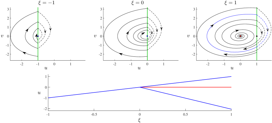
Figure 9.2: An illustration of HLB 11 for the impacting system (9.12) with $(\tau,\delta,r)=(0.2,1,0.5)$. By increasing the value of $\xi$ a virtual unstable focus becomes admissible and a stable limit cycle is created.

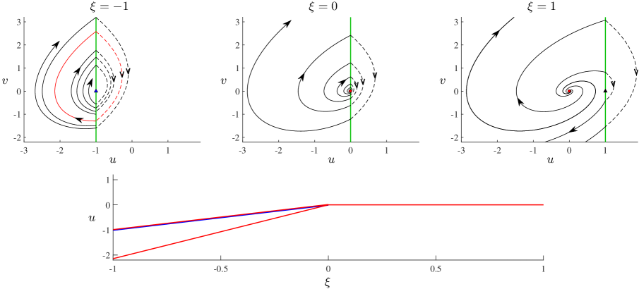
Figure 9.3: An illustration of HLB 12 for the impacting system (9.12) with $(\tau,\delta,r)=(0.8,1,0.5)$. By decreasing the value of $\xi$ an admissible unstable focus undergoes a BEB with the impacting surface and an unstable limit cycle is created.

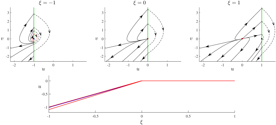
Figure 9.4: An illustration of HLB 13 for the impacting system (9.12) with $(\tau,\delta,r)=(2.5,1,0.5)$. By decreasing the value of $\xi$ an admissible unstable node undergoes a BEB with the impacting surface and an unstable limit cycle is created.

As an example we consider the linear impact oscillator

$$\begin{split}\dot{u}&=v,\\ \dot{v}&=-\delta u+\tau v,\\ v&\mapsto-rv,{\rm~{}when~{}}u=\xi.\end{split}$$ (9.12)

where $\tau,\delta,\xi\in\mathbb{R}$ and $r\geq 0$ are constants. Here $u(t)$ represents the displacement of the oscillator from its equilibrium position. The oscillator undergoes instantaneous impacts with restitution coefficient $r$ whenever $u(t)=\xi$.

We treat $\xi$ as the main bifurcation parameter and apply Theorems 9.2–9.4 via the substitution $(x,y;\mu)=(u-\xi,v;\xi)$. Notice $\tau$ and $\delta$ are the trace and determinant of ${\rm D}F(0,0;0)$. Also

$$\alpha =\ln{r}+\frac{\pi\tau}{\sqrt{4\delta-\tau^{2}}}, \beta =\delta, \gamma =r.$$

Here we briefly consider parameter values that illustrate HLBs 11–13. Specifically we fix

$$\delta =1, r=0.5,$$

and consider different values of $\tau$. We study the change in the dynamics as the value of $\xi$ changes sign, but (9.12) is invariant when $u$, $v$, and $\xi$ are scaled by a positive constant, hence it suffices to consider $\xi\in\{-1,0,1\}$. With $\tau=0.2$ the regular equilibrium is an unstable focus and $\alpha<0$. In accordance with Theorem 9.2, a stable limit cycle exists when the focus is admissible, Fig. 9.2. With $\tau=0.8$, now $\alpha>0$ and by Theorem 9.3 an unstable limit cycle exists when the focus is virtual, Fig. 9.3. Finally with $\tau=2.5$ the regular equilibrium is an unstable node. Again $\alpha>0$ and so by Theorem 9.4 an unstable limit cycle exists when the node is virtual, Fig. 9.4.

9.2 Impulsive systems — HLB 14

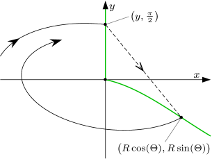
Figure 9.5: Part of a typical orbit of the impulsive system (9.13) with (9.16).

Here we consider ODEs combined with an impulse law (defined below) that is applied when orbits reach the positive $y$-axis, see Fig. 9.5. We suppose the origin is a focus equilibrium of the ODEs and that here the impulse is zero. The origin is a stationary solution that may change stability and emit a limit cycle under parameter variation; this is HLB 14. The bifurcation can be generalised to allow several independent vector fields and impulse laws each acting in regions that share a vertex at the origin, AkKa17 ; Ak05 ; HuYa12 .

If the impulse law maps points to the negative $y$-axis we recover the impacting scenario of §9.1, although here the regular equilibrium is fixed at the origin whereas for HLBs 11–13 the bifurcation is triggered by the collision of a regular equilibrium with $x=0$ (i.e. a BEB). HLB 14 was described in HeMo17 for an abstract impacting system although there the nonlinearity in the ODEs is cubic, not quadratic, and consequently the amplitude of the limit cycle is asymptotically proportional to square-root of the parameter change.

Let us clarify the class of impulsive systems under consideration. We write the ODEs as

$$\begin{bmatrix}\dot{x}\\ \dot{y}\end{bmatrix}=F(x,y;\mu),{\rm~{}until~{}}x=0,\,y>0,$$ (9.13)

with

$$F(x,y;\mu)=\begin{bmatrix}f(x,y;\mu)\\ g(x,y;\mu)\end{bmatrix},$$

where $f$ and $g$ are smooth functions. We assume

$$f(0,0;\mu)=g(0,0;\mu),$$ (9.14)

for all values of $\mu$ in a neighbourhood $0$ so that (9.13) has a regular equilibrium fixed at the origin. We assume this equilibrium is a focus and that its associated Jacobian matrix is in real-Jordan form:

$${\rm D}F(0,0;\mu)=\begin{bmatrix}\lambda(\mu)&\omega(\mu)\\ -\omega(\mu)&\lambda(\mu)\end{bmatrix},$$ (9.15)

where $\lambda(\mu)\in\mathbb{R}$ and $\omega(\mu)>0$. This assumption is included so that Theorem 9.26, given below, is reasonably succinct. As with other results in this paper, in order to apply Theorem 9.26 to a particular model one would use a change of variables to satisfy (9.15).

To state Theorem 9.26 we use polar coordinates: $x=r\cos(\theta)$, $y=r\sin(\theta)$. The positive $y$-axis corresponds to $\theta=\frac{\pi}{2}$ and we assume $\theta\in\mathopen{}\mathclose{{}\left(-\frac{3\pi}{2},\frac{\pi}{2}}\right]$. Since $\omega>0$, orbits following the vector field $F$ rotate clockwise (at least near the origin). Thus the value of $\theta$ decreases with time until $\theta=-\frac{3\pi}{2}$ when we reset it to $\theta=\frac{\pi}{2}$ and apply the impulse law. We write the impulse law as

$$\mathopen{}\mathclose{{}\left(y,\frac{\pi}{2}}\right)\mapsto\mathopen{}\mathclose{{}\left(R(y;\mu),\Theta(y;\mu)}\right).$$ (9.16)

where $R$ and $\Theta$ are smooth functions. We assume $R(0;\mu)=0$, for all $\mu$, so that the impulse is zero at the origin, and let

$$\gamma(\mu)=\frac{\partial R}{\partial y}(0;\mu).$$ (9.17)

We also assume $\Theta(y;\mu)\in\mathopen{}\mathclose{{}\left(\frac{-3\pi}{2},\frac{\pi}{2}}\right)$, and let

$$\phi(\mu)=\Theta(0;\mu).$$ (9.18)

Thus the impulse law can be written as

$$\mathopen{}\mathclose{{}\left(y,\frac{\pi}{2}}\right)\mapsto\mathopen{}\mathclose{{}\left(\gamma y+O\mathopen{}\mathclose{{}\left(y^{2}}\right),\phi+O(y)}\right).$$ (9.19)

Upon subsequent evolution via (9.13), the orbit returns to $\theta=\frac{\pi}{2}$ at $r=\gamma y{\rm e}^{\lambda t}+O\mathopen{}\mathclose{{}\left(y^{2}}\right)$, where the evolution time is $t=\frac{1}{\omega}\mathopen{}\mathclose{{}\left(\phi+\frac{3\pi}{2}}\right)+O(y)$. Thus one revolution corresponds to $y\mapsto{\rm e}^{\Lambda}y+O\mathopen{}\mathclose{{}\left(y^{2}}\right)$, where

$$\Lambda(\mu)=\ln(\gamma(\mu))+\frac{\lambda(\mu)}{\omega(\mu)}\mathopen{}\mathclose{{}\left(\phi(\mu)+\frac{3\pi}{2}}\right).$$ (9.20)

This shows that the stability of the origin is governed by the sign of $\Lambda$. For HLB 14 we assume $\Lambda(0)=0$ and $\beta\neq 0$ where

$$\beta=\frac{d\Lambda}{d\mu}(0).$$ (9.21)

Some work is required to state the non-degeneracy coefficient $\alpha$. First we write

$$\begin{split}f(x,y;\mu)&=\lambda(\mu)x+\omega(\mu)y\\ &\quad+a_{1}x^{2}+a_{2}xy+a_{3}y^{2}+o\mathopen{}\mathclose{{}\left(\mathopen{}\mathclose{{}\left(|x|+|y|+|\mu|}\right)^{2}}\right),\\ g(x,y;\mu)&=-\omega(\mu)x+\lambda(\mu)y\\ &\quad+b_{1}x^{2}+b_{2}xy+b_{3}y^{2}+o\mathopen{}\mathclose{{}\left(\mathopen{}\mathclose{{}\left(|x|+|y|+|\mu|}\right)^{2}}\right),\end{split}$$ (9.22)

for constants $a_{1},\ldots,b_{3}\in\mathbb{R}$. In polar coordinates (9.13) may be written as

$$\begin{split}\dot{r}&=\lambda(\mu)r+r^{2}\mathcal{F}(\theta)+o\mathopen{}\mathclose{{}\left(\mathopen{}\mathclose{{}\left(r+|\mu|}\right)^{2}}\right),\\ \dot{\theta}&=-\omega(\mu)+r\mathcal{G}(\theta)+o\mathopen{}\mathclose{{}\left(r+|\mu|}\right),\end{split}$$ (9.23)

where

$$\begin{split}\mathcal{F}(\theta)&=a_{1}\cos^{3}(\theta)+(a_{2}+b_{1})\cos^{2}(\theta)\sin(\theta)\\ &\quad+(a_{3}+b_{2})\cos(\theta)\sin^{2}(\theta)+b_{3}\sin^{3}(\theta),\\ \mathcal{G}(\theta)&=b_{1}\cos^{3}(\theta)+(b_{2}-a_{1})\cos^{2}(\theta)\sin(\theta)\\ &\quad+(b_{3}-a_{2})\cos(\theta)\sin^{2}(\theta)-a_{3}\sin^{3}(\theta).\end{split}$$ (9.24)

Then

$$\alpha =\frac{\frac{\partial^{2}R}{\partial y^{2}}(0;0)}{2\gamma(0)}+\frac{\lambda}{\omega}\,\frac{\partial\Theta}{\partial y}(0;0)$$

$$\quad+\frac{1}{\omega}\,{\rm e}^{\frac{-3\pi\lambda}{2\omega}}\int_{\frac{-3\pi}{2}}^{\phi(0)}{\rm e}^{\frac{-\lambda\theta}{\omega}}\mathopen{}\mathclose{{}\left(\mathcal{F}(\theta)+\frac{\lambda}{\omega}\,\mathcal{G}(\theta)}\right)\,d\theta.$$ (9.25)

The integral in (9.25) can be evaluated explicitly but we have left it in integral form for brevity.

Theorem 9.5 (HLB 14).

Consider (9.13) with (9.16), where $F$ is $C^{2}$, $R$ is $C^{2}$, and $\Theta$ is $C^{1}$. Suppose (9.14) and (9.15) are satisfied, $\Lambda(0)=0$, and $\beta>0$. In a neighbourhood of $(x,y;\mu)=(0,0;0)$,

1. the origin is the unique stationary solution and is stable for $\mu<0$ and unstable for $\mu>0$,

2. if $\alpha<0$ [$\alpha>0$] there exists a unique stable [unstable] limit cycle for $\mu>0$ [$\mu<0$], and no limit cycle for $\mu<0$ [$\mu>0$].

The amplitude of the limit cycle is asymptotically proportional to $|\mu|$, and its period is

$$T=\frac{1}{\omega(0)}\mathopen{}\mathclose{{}\left(\phi(0)+\frac{3\pi}{2}}\right)+O(\mu).$$ (9.26)

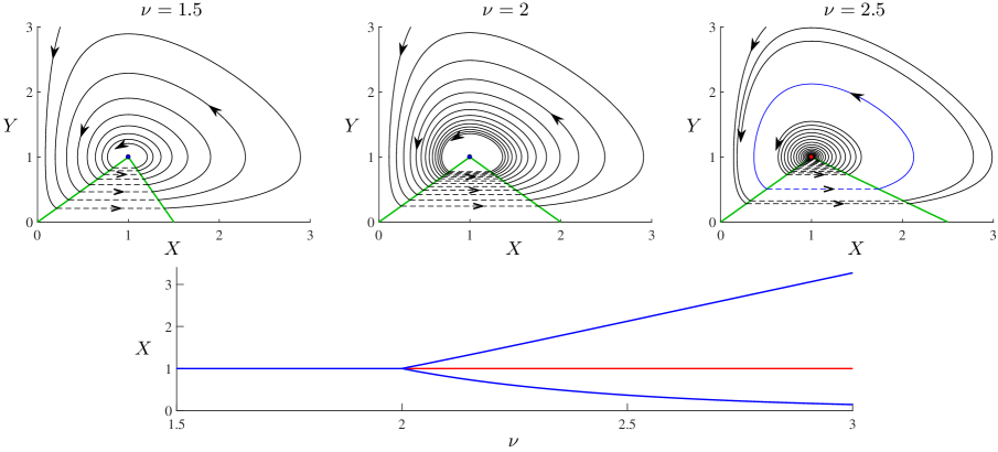
Figure 9.6: An illustration of HLB 14 for the Lotka-Volterra system (9.27) with impulse (9.28) using the parameter values (9.29). By increasing the value of $\nu$ the equilibrium $(X^{*},Y^{*})=\mathopen{}\mathclose{{}\left(\frac{c}{d},\frac{a}{b}}\right)$ loses stability when $\nu=2$ and a stable limit cycle is created.

To illustrate Theorem 9.26 we study a simple Lotka-Volterra system with impulse. Such systems model the populations of competing species where impulses correspond to poison drops, insect outbreaks, or other abrupt events such as the artificial addition of species members for control purposes LiZh05 ; LiCh03 ; LiRo98 ; NiPe09 .

Consider

$$\begin{split}\dot{X}&=aX-bXY,\\ \dot{Y}&=-cY+dXY,\end{split}$$ (9.27)

where $X$ and $Y$ represent prey and predator populations respectively, and $a,b,c,d>0$. This system has a saddle equilibrium at the origin, a centre equilibrium at $(X^{*},Y^{*})=\mathopen{}\mathclose{{}\left(\frac{c}{d},\frac{a}{b}}\right)$, and an uncountable family of periodic orbits encircling $(X^{*},Y^{*})$ throughout the first quadrant, $X,Y>0$.

Now suppose that whenever a forward orbit of (9.27) intersects the line segment connecting the two equilibria, the value $\nu\mathopen{}\mathclose{{}\left(X^{*}-X}\right)$ is added to the prey population, where $\nu>0$ is a constant. That is,

$$(X,Y)\mapsto\mathopen{}\mathclose{{}\left(X+\nu\mathopen{}\mathclose{{}\left(\frac{c}{d}-X}\right),Y}\right),$$ (9.28)

where $X\in\mathopen{}\mathclose{{}\left(0,\frac{c}{d}}\right)$, and $Y=\frac{ad}{bc}X$. This particular impulse law provides a succinct example of HLB 14. Fig. 9.6 shows phase portraits and a bifurcation diagram using

$$a=b=c=d=1,$$ (9.29)

for which HLB 14 occurs at $\nu=2$.

To apply Theorem 9.26 using the particular parameter values (9.29), we perform the coordinate change

$$\begin{split}x&=X-Y,\\ y&=-X-Y+2.\end{split}$$

Then (9.27) with (9.29) becomes

$$\begin{split}\dot{x}&=y+\frac{x^{2}-y^{2}}{2},\\ \dot{y}&=-x,\end{split}$$

and in polar coordinates the impulse law is

$$\begin{split}R(y)&=y\sqrt{1-\nu+\frac{\nu^{2}}{2}},\\ \Theta(y)&=\tan^{-1}\mathopen{}\mathclose{{}\left(\frac{2}{\nu}-1}\right).\end{split}$$

Here $\Lambda=\frac{1}{2}\ln\mathopen{}\mathclose{{}\left(1-\nu+\frac{\nu^{2}}{2}}\right)$ and so $\Lambda=0$ when $\nu=2$. The transversality condition is satisfied because $\beta=\frac{d\Lambda}{d\nu}(2)=\frac{1}{2}$. To evaluate $\alpha$ observe that the first two terms in (9.25) are zero. In the integral we have $\lambda=0$, $\omega=1$, and

$$a_{1} =\frac{1}{2}, a_{2} =0, a_{3} =-\frac{1}{2},$$

$$b_{1} =0, b_{2} =0, b_{3} =0,$$

and so

$$\alpha=\frac{1}{2}\int_{\frac{-3\pi}{2}}^{0}\cos^{3}(\theta)-\cos(\theta)\sin^{2}(\theta)\,d\theta=-\frac{1}{6}.$$

Thus Theorem 9.26 tells us that a stable limit cycle is created at $\nu=2$ and exists for $\nu>2$, as seen in Fig. 9.6.

10 Switching with hysteresis and time delay

Here we suppose the Filippov system

$$\begin{bmatrix}\dot{x}\\ \dot{y}\end{bmatrix}=\begin{cases}F_{L}(x,y),&x<0,\\ F_{R}(x,y),&x>0,\end{cases}$$ (10.1)

has a stable pseudo-equilibrium or invisible-invisible two-fold at the origin. We analyse the limit cycle created by adding hysteresis or time delay to the switching condition (called border-splitting in MaLa12 ). The hysteretic system is

$$\begin{bmatrix}\dot{x}\\ \dot{y}\end{bmatrix}=\begin{cases}F_{L}(x,y),&{\rm until~{}}x=\mu,\\ F_{R}(x,y),&{\rm until~{}}x=-\mu,\end{cases}$$ (10.2)

and the delayed system is

$$\begin{bmatrix}\dot{x}(t)\\ \dot{y}(t)\end{bmatrix}=\begin{cases}F_{L}(x(t),y(t)),&x(t-\mu)<0,\\ F_{R}(x(t),y(t)),&x(t-\mu)>0,\end{cases}$$ (10.3)

where in each case $\mu\geq 0$ is assumed to be small in the analysis below. As usual we write

$$F_{J}(x,y)=\begin{bmatrix}f_{J}(x,y)\\ g_{J}(x,y)\end{bmatrix},$$ (10.4)

for each $J\in\{L,R\}$.

When the origin is a two-fold it must be stable for a limit cycle to be created. This is because hysteresis and delay produce an instability. Similarly when the origin is a pseudo-equilibrium it must belong to an attracting sliding region for a limit cycle to be created. In this case the stability of the limit cycle (with $\mu>0$) matches that of the pseudo-equilibrium (with $\mu=0$).

Such limit cycles are ubiquitous in relay control systems that use switches to affect control tasks Ts84 . Sliding mode control employs rapid switching to maintain the system state near a desired manifold PeBa02 ; UtGu09 ; Ut92 . The rapid switching motion tends to sliding motion as the switching frequency tends to infinity. In reality the switching frequency is finite and the system state ‘chatters’ about the switching manifold. Chattering can be periodic forming a limit cycle of a size that directly correlates to discrepancies of the system from its idealised (infinite frequency) limit Bo09 ; Ja93 . Note that chattering typically causes undue strain and wear on mechanical components so control algorithms that minimise chattering are usually preferred.

A stable pseudo-equilibrium is usually the desired state of a first-order sliding mode control system. Bang-bang controllers use hysteresis (most simply with no backlash or deadzone) resulting in a limit cycle MaHa17 (see LiYu08 ; LoMi88 in the case of delay). Invisible-invisible two-folds correspond to second-order sliding mode control BaPi03 . Calculations of the resulting limit cycle can be found in Ma17 for hysteresis and in Ko17 ; LePu06 ; LiYu13 for delay (see also Si06 for large delay). Below we treat a pseudo-equilibrium in §10.1 and a two-fold in §10.2.

10.1 Perturbing a pseudo-equilibrium — HLBs 15–16

For a system of the form (10.1), let

$$a_{0L} =f_{L}(0,0), a_{0R} =f_{R}(0,0).$$ (10.5)

We suppose $a_{0R}<0<a_{0L}$ so that the origin belongs to an attracting sliding region. We also suppose that the origin is a pseudo-equilibrium, hence

$$\mathopen{}\mathclose{{}\left(f_{L}g_{R}-f_{R}g_{L}\middle)}\right|_{x=y=0}=0.$$ (10.6)

The stability of the origin is governed by the sign of

$$\alpha=\frac{\partial}{\partial y}\mathopen{}\mathclose{{}\left(f_{L}g_{R}-f_{R}g_{L}\middle)}\right|_{x=y=0}\,.$$ (10.7)

The following theorems describe a local limit cycle for the hysteretic and delayed systems (10.2)–(10.3). As with other results in this paper, the results are proved by analysing a Poincaré map. This is sufficient to completely describe the local dynamics of the hysteretic system. The delayed system, however, is infinite dimensional Er09 ; HaLu93 . The limit cycle obtained is only unique among orbits for which the time between any two switches is no less than the delay $\mu$. For Glass networks with delay, Edwards et. al. EdVa07 prove the limit cycle is unique under the assumption that the initial condition history includes no switches.

Theorem 10.1 (HLB 15).

Consider the hysteretic system (10.2) where $F_{L}$ and $F_{R}$ are $C^{2}$. Suppose $a_{0R}<0<a_{0L}$ and (10.6) is satisfied. In a neighbourhood of $(x,y;\mu)=(0,0;0)$, if $\alpha<0$ [$\alpha>0$] there exists a unique stable [unstable] limit cycle for $\mu>0$. The minimum and maximum $x$-values of the limit cycle are $\pm\mu$ and its period is

$$T=\mathopen{}\mathclose{{}\left(\frac{2}{a_{0L}}-\frac{2}{a_{0R}}}\right)\mu+O\mathopen{}\mathclose{{}\left(\mu^{2}}\right).$$ (10.8)

Theorem 10.2 (HLB 16).

Consider the delayed system (10.3) where $F_{L}$ and $F_{R}$ are $C^{2}$. Suppose $a_{0R}<0<a_{0L}$ and (10.6) is satisfied. In a neighbourhood of $(x,y;\mu)=(0,0;0)$, treating only orbits for which times between consecutive switches is not less than $\mu$, if $\alpha<0$ [$\alpha>0$] there exists a unique stable [unstable] limit cycle for $\mu>0$. The minimum and maximum $x$-values of the limit cycle are asymptotically proportional to $\mu$, and its period is

$$T=\mathopen{}\mathclose{{}\left(2-\frac{a_{0L}}{a_{0R}}-\frac{a_{0R}}{a_{0L}}}\right)\mu+O\mathopen{}\mathclose{{}\left(\mu^{2}}\right).$$ (10.9)

As an example we use the observer canonical form for a two-dimensional relay control system Bu01 :

$$\begin{bmatrix}\dot{x}\\ \dot{y}\end{bmatrix}=\begin{bmatrix}\tau&1\\ -\delta&0\end{bmatrix}\begin{bmatrix}x\\ y\end{bmatrix}-{\rm sgn}(x)\begin{bmatrix}b_{1}\\ b_{2}\end{bmatrix}.$$ (10.10)

This system is of the form (10.1). If $b_{1}>0$, then the interval $-b_{1}<y<b_{1}$ is an attracting sliding region and the origin is a pseudo-equilibrium. If also $b_{2}>0$, then the origin is stable. In this case the inclusion of hysteresis or delay generates a stable limit cycle in accordance with Theorems 10.8 and 10.9 as shown in Figs. 10.1 and 10.2 for the parameter values

$$\tau =-0.5, \delta =1, b_{1} =1, b_{2} =1.$$ (10.11)

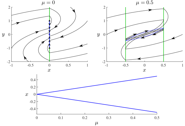
Figure 10.1: An illustration of HLB 15 for the canonical relay control system (10.10) using hysteresis of the form (10.2) and the parameter values (10.11). By increasing the value of $\mu$ from $0$, a stable pseudo-equilibrium is replaced by a limit cycle with period asymptotically proportional to $\mu$.

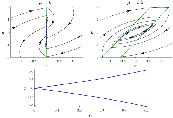
Figure 10.2: An illustration of HLB 16 for the canonical relay control system (10.10) using delay of the form (10.3) and the parameter values (10.11). The green lines indicate where switches occur.

10.2 Perturbing a two-fold — HLBs 17–18

Here we let

$$a_{2J} =\frac{\partial f_{J}}{\partial y}(0,0), b_{0J} =g_{J}(0,0),$$ (10.12)

and

$$\gamma_{J}=a_{2J}b_{0J},$$ (10.13)

for each $J\in\{L,R\}$. We also define

$$\kappa=\frac{b_{0L}}{a_{2L}}-\frac{b_{0R}}{a_{2R}}.$$ (10.14)

We suppose the origin is an invisible fold for both the left and right half-systems of (10.1). That is

$$f_{L}(0,0)=f_{R}(0,0)=0,$$ (10.15)

and $\gamma_{L}>0$ and $\gamma_{R}<0$. We assume $a_{2L}a_{2R}>0$, so that orbits of both half-systems involve the same direction of rotation. Then, as with HLB 7, the stability of the two-fold is governed by the sign of

$$\alpha=\sigma_{{\rm fold},L}-\sigma_{{\rm fold},R}\,,$$ (10.16)

using the formula (4.12).

Theorem 10.3 (HLB 17).

Consider the hysteretic system (10.2) where $F_{L}$ and $F_{R}$ are $C^{3}$. Suppose (10.15) is satisfied, $\gamma_{L}>0$, $\gamma_{R}<0$, and $a_{2L}a_{2R}>0$. In a neighbourhood of $(x,y;\mu)=(0,0;0)$, if $\alpha<0$ [$\alpha>0$] there exists a unique stable limit cycle [no limit cycle] for $\mu>0$. The minimum and maximum $x$-values of the limit cycle are asymptotically proportional to $\mu^{\frac{2}{3}}$, the minimum and maximum $y$-values are asymptotically proportional to $\mu^{\frac{1}{3}}$, and its period is

$$T=\mathopen{}\mathclose{{}\left|\frac{2}{b_{0L}}-\frac{2}{b_{0R}}}\right|\mathopen{}\mathclose{{}\left(\frac{3\kappa\mu}{|\alpha|}}\right)^{\frac{1}{3}}+o\mathopen{}\mathclose{{}\left(\mu^{\frac{1}{3}}}\right).$$ (10.17)

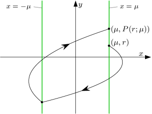
Figure 10.3: An illustration of the Poincaré map $P$ associated with HLB 17.

The interesting cube-root asymptotics are explained by a Poincaré map. Given $r\in\mathbb{R}$, suppose the forward orbit of $(x,y)=(\mu,r)$ undergoes a switch on $x=-\mu$, then a switch on $x=\mu$, as in Fig. 10.3. Let $P(r;\mu)$ denote the $y$-value of the second switch. In Appendix G we show that

$$P(r;\mu)=\sqrt{r^{2}+4\kappa\mu+\frac{4\alpha}{3}\,r^{3}+E},$$ (10.18)

where $E$ is an error term. By solving the fixed point equation $P(r;\mu)=r$ we obtain $r=\sqrt{\frac{3\kappa}{|\alpha|}}\,\mu^{\frac{1}{3}}$, to leading order. To deal with the unique technical difficulties that arise in deriving (10.18), this equation is obtained in Appendix G by non-constructive means. A different form for $P(r;\mu)$ is obtained in Ma17 by assuming a priori that the value of $r$ is not too small relative to $\mu$. This form can be obtained from (10.18) as follows. Assume $r>0$ and $r=O\big{(}\mu^{\frac{1}{3}}\big{)}$ (this sufficient to obtain the limit cycle). Then a linear approximation to the square-root produces

$$P(r;\mu)=r+\frac{2\kappa\mu}{r}+\frac{2\alpha}{3}r^{2}+o\mathopen{}\mathclose{{}\left(r^{2}}\right),$$

which is the form obtained in Ma17 .

Theorem 10.4 (HLB 18).

Consider the delayed system (10.3) where $F_{L}$ and $F_{R}$ are $C^{3}$. Suppose (10.15), $\gamma_{L}>0$, $\gamma_{R}<0$, and $a_{2L}a_{2R}>0$. In a neighbourhood of $(x,y;\mu)=(0,0;0)$, treating only orbits for which times between consecutive switches is not less than $\mu$, if $\alpha<0$ [$\alpha>0$] there exists a unique stable limit cycle [no limit cycle] for $\mu>0$. The minimum and maximum $x$-values of the limit cycle are asymptotically proportional to $\mu$, the minimum and maximum $y$-values are asymptotically proportional to $\sqrt{\mu}$, and its period is

$$T=\mathopen{}\mathclose{{}\left|\frac{2}{b_{0L}}-\frac{2}{b_{0R}}}\right|\sqrt{\frac{3\mathopen{}\mathclose{{}\left(a_{2L}+a_{2R}}\right)\kappa}{2|\alpha|}}\,\sqrt{\mu}+o\mathopen{}\mathclose{{}\left(\sqrt{\mu}}\right).$$ (10.19)

To illustrate Theorems 10.17 and 10.19 we consider a linear oscillator with discontinuous forcing:

$$m\ddot{x}+b\dot{x}+kx=F_{\rm apply}\,.$$ (10.20)

Let $F>0$ be a constant and suppose the applied force is given by $F_{\rm apply}=F$ until $x=\mu$, and $F_{\rm apply}=-F$ until $x=-\mu$. By writing the system as

$$\begin{split}\dot{x}&=y,\\ \dot{y}&=\begin{cases}-\frac{k}{m}\,x-\frac{b}{m}\,y+\frac{F}{m},&{\rm until~{}}x=\mu,\\ -\frac{k}{m}\,x-\frac{b}{m}\,y-\frac{F}{m},&{\rm until~{}}x=-\mu,\end{cases}\end{split}$$ (10.21)

we can apply Theorem 10.17 directly. Here the non-degeneracy coefficient is $\alpha=\frac{-2b}{F}$, so a positive damping coefficient $b$ guarantees the creation of a stable limit cycle. Fig. 10.4 shows a bifurcation diagram and phase portraits using

$$m =1, b =0.5, k =1, F =1.$$ (10.22)

Fig. 10.5 shows a bifurcation diagram and phase portraits for the analogous delayed system

$$\begin{split}\dot{x}(t)&=y(t),\\ \dot{y}(t)&=\begin{cases}-\frac{k}{m}\,x(t)-\frac{b}{m}\,y(t)+\frac{F}{m},&x(t-\mu)<0,\\ -\frac{k}{m}\,x(t)-\frac{b}{m}\,y(t)-\frac{F}{m},&x(t-\mu)>0.\end{cases}\end{split}$$ (10.23)

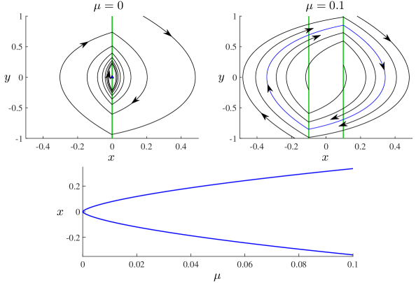
Figure 10.4: An illustration of HLB 17 for a linear oscillator with hysteretic discontinuous forcing, (10.21) with (10.22). By increasing the value of $\mu$ from $0$, a stable invisible-invisible two-fold is replaced by a limit cycle with period asymptotically proportional to $\mu^{\frac{1}{3}}$.

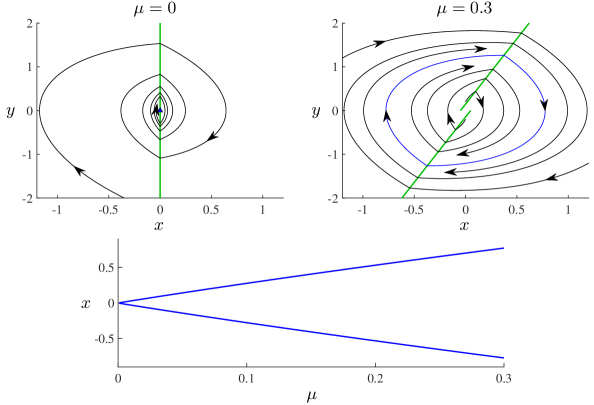
Figure 10.5: An illustration of HLB 18 for a linear oscillator with delayed discontinuous forcing, (10.23) with (10.22).

11 Other mechanisms for limit cycle creation

11.1 Intersecting switching manifolds — HLB 19

Many systems involve multiple switches; examples include gene networks EdGl14 ; GoSa02 and relay control systems Ut92 . In phase space, two switching manifolds generically intersect on a codimension-two surface. Determining an appropriate sliding vector field on such a surface is surprisingly difficult in a general setting, see DiDi17 ; Je14c ; JeKa18 for recent developments, however here we are only concerned with two-dimensional systems for which two switching manifolds can be expected to intersect at a point. The dynamics near two transversally intersecting switching manifolds, depends on the direction of the vector field in each of the four regions bounded by the switching manifolds GuHa15 ; Je16f . Here we suppose orbits spiral around the intersection point, as in Fig. 11.1. Then the intersection point is a stationary solution and it may emit a limit cycle when its stability changes under parameter variation.

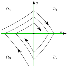
Figure 11.1: Parts of typical orbits of (11.1) subject to (11.2).

We assume the switching manifolds coincide with the coordinate axes, and define

$$\begin{split}\Omega_{1}&=\{(x,y)\,|\,x>0,\,y>0\},\\ \Omega_{2}&=\{(x,y)\,|\,x>0,\,y<0\},\\ \Omega_{3}&=\{(x,y)\,|\,x<0,\,y<0\},\\ \Omega_{4}&=\{(x,y)\,|\,x<0,\,y>0\}.\end{split}$$

We write the system as

$$\begin{bmatrix}\dot{x}\\ \dot{y}\end{bmatrix}=\begin{cases}F_{1}(x,y;\mu),&(x,y)\in\Omega_{1}\,,\\[-3.69885pt] \hskip 22.76219pt\vdots&\hskip 27.0301pt\vdots\\[-3.69885pt] F_{4}(x,y;\mu),&(x,y)\in\Omega_{4}\,,\end{cases}$$ (11.1)

where

$$F_{j}(x,y;\mu)=\begin{bmatrix}f_{j}(x,y;\mu)\\ g_{j}(x,y;\mu)\end{bmatrix},$$

is smooth for each $j=1,\ldots,4$. We suppose

$$f_{1}(0,0;0) >0, g_{1}(0,0;0) <0,$$ (11.2)

$$f_{2}(0,0;0) <0, g_{2}(0,0;0) <0,$$

$$f_{3}(0,0;0) <0, g_{3}(0,0;0) >0,$$

$$f_{4}(0,0;0) >0, g_{4}(0,0;0) >0,$$

so that nearby orbits spiral clockwise around the origin.

Suppose the forward orbit of $(x,y)=(0,r)$, with $r>0$, next intersects the positive $y$-axis at some point $(0,P(r;\mu))$. It is a simple exercise to show that $P(r;\mu)=\Lambda(\mu)r+O\mathopen{}\mathclose{{}\left(r^{2}}\right)$, where

$$\Lambda(\mu)=\frac{m_{2}(\mu)m_{4}(\mu)}{m_{1}(\mu)m_{3}(\mu)},$$ (11.3)

and

$$m_{j}(\mu)=\frac{g_{j}(0,0;\mu)}{f_{j}(0,0;\mu)},$$ (11.4)

represents the slope $\frac{dy}{dx}$ of $F_{j}$ evaluated at the origin. Thus the stability of the origin is governed by the sign of $\ln(\Lambda)$. In order for HLB 19 to occur at $\mu=0$ we assume $\Lambda(0)=1$. The transversality condition is $\beta\neq 0$, where

$$\beta=\frac{d\Lambda}{d\mu}(0).$$ (11.5)

Also let

$$\xi_{j}(\mu)=\frac{1}{f_{j}}\mathopen{}\mathclose{{}\left(\frac{g_{j}}{f_{j}}\frac{\partial f_{j}}{\partial y}-\mathopen{}\mathclose{{}\left(\frac{\partial f_{j}}{\partial x}+\frac{\partial g_{j}}{\partial y}}\right)+\frac{f_{j}}{g_{j}}\frac{\partial g_{j}}{\partial x}\middle)}\right|_{x=y=0},\\$$ (11.6)

for each $j$, and

$$\alpha=\mathopen{}\mathclose{{}\left(\frac{\xi_{1}-\xi_{2}}{m_{1}}+\frac{\xi_{3}-\xi_{4}}{m_{4}}\middle)}\right|_{\mu=0}\,.$$ (11.7)

Theorem 11.1 (HLB 19).

Consider (11.1) where $F_{j}$ is $C^{2}$ for each $j=1,\ldots,4$. Suppose (11.2) is satisfied, $\Lambda(0)=1$, and $\beta>0$. In a neighbourhood of $(x,y;\mu)=(0,0;0)$,

1. the origin is the unique stationary solution and is stable for $\mu<0$ and unstable for $\mu>0$,

2. if $\alpha<0$ [$\alpha>0$] there exists a unique stable [unstable] limit cycle for $\mu>0$ [$\mu<0$], and no limit cycle for $\mu<0$ [$\mu>0$].

The minimum and maximum $x$ and $y$-values of the limit cycle are asymptotically proportional to $|\mu|$, and its period is

$$T=\frac{2\beta}{|\alpha|}\mathopen{}\mathclose{{}\left(\frac{-1}{g_{1}}+\frac{1}{f_{2}m_{1}}-\frac{1}{f_{3}m_{4}}+\frac{1}{g_{4}}\middle)}\right|_{x=y=\mu=0}|\mu|+o(\mu).$$ (11.8)

HLB 19 occurs in a version of the Wilson-Cowan model for the aggregated dynamics of a large network of excitatory and inhibitory neurons:

$$\begin{split}\dot{u}&=-u+H(u-av-b),\\ \tau\dot{v}&=-v+H(u-cv-d).\end{split}$$ (11.9)

Here $u(t)$ represents the average activity (e.g. voltage) of the neurons, $v(t)$ is a recovery variable, and $a,b,c,d,\tau>0$ are parameters. As in HaEr15 , we take the firing rate function $H$ to be the Heaviside function. This system has two switching manifolds, $u=av+b$ and $u=cv+d$, and for typical parameter values orbits spiral around their unique point of intersection. With $\tau$ as the primary bifurcation parameter, Fig. 11.2 shows a bifurcation diagram and representative phase portraits using

$$a =2, b =0.05, c =0.25, d =0.3,$$ (11.10)

as given in HaEr15 .

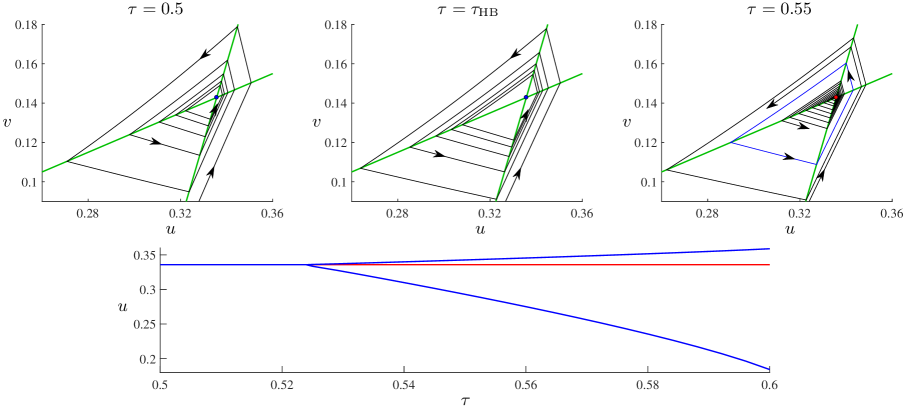
Figure 11.2: An illustration of HLB 19 for the Wilson-Cowan model (11.9) with (11.10). By increasing the value of $\tau$, the stable stationary solution located at the intersection of the two switching manifolds loses stability when $\tau=\tau_{\rm HB}\approx 0.5240$ and emits a stable limit cycle.

In HaEr15 the authors use a Poincaré map to determine when HLB 19 occurs. Here use Theorem 11.8 to obtain the same result and show that the limit cycle is stable by numerically evaluating (11.7). To do this we employ the change of variables

$$\begin{split}x&=u-cv-d,\\ y&=u-av-b.\end{split}$$ (11.11)

and, assuming $a>c$, scale time by

$$t\mapsto\frac{t}{(a-c)\tau},$$

to achieve additional simplification. The system is then given by (11.1) with

$$\begin{split}F_{1}(x,y)&=F_{3}(x,y)+(a-c)\begin{bmatrix}\tau-c\\ \tau-a\end{bmatrix},\\ F_{2}(x,y)&=F_{3}(x,y)-(a-c)\begin{bmatrix}c\\ a\end{bmatrix},\\ F_{3}(x,y)&=\begin{bmatrix}-(a\tau-c)&-c(1-\tau)\\ a(1-\tau)&-(a-c\tau)\end{bmatrix}\begin{bmatrix}x\\ y\end{bmatrix}\\ &\quad-\begin{bmatrix}c(b-d)+(ad-bc)\tau\\ a(b-d)+(ad-bc)\tau\end{bmatrix},\\ F_{4}(x,y)&=F_{3}(x,y)+(a-c)\begin{bmatrix}\tau\\ \tau\end{bmatrix}.\end{split}$$ (11.12)

By numerically evaluating (11.3) we find that $\Lambda=1$ when $\tau=\tau_{\rm HB}\approx 0.5240$ (to four decimal places). Also $\alpha\approx-8.47$ and $\beta\approx 9.53$, using $\mu=\tau-\tau_{\rm HB}$. Since $\alpha<0$ the limit cycle is stable (as shown in Fig. 11.2).

11.2 A square-root singularity — HLB 20

The leading-order dynamics near some grazing bifurcations (where a limit cycle attains a tangential intersection with a switching manifold) are described by piecewise-smooth Poincaré maps involving a square-root singularity ChOt94 ; No91 . In this section we study the analogous class of ODEs. Specifically we consider

$$\begin{bmatrix}\dot{x}\\ \dot{y}\end{bmatrix}=F(x,y;S(x);\mu),$$ (11.13)

where $F$ is a smooth function of its four components, and

$$S(x)=\begin{cases}0,&x\leq 0,\\ \sqrt{x},&x\geq 0.\end{cases}$$ (11.14)

This is motivated by the work NiCa16 where an ODE system with a square-root singularity is introduced to model the averaged behaviour of a large number of coupled neurons.

We suppose (11.13) exhibits a BEB at the origin when $\mu=0$. Thus

$$f(0,0;0;0)=g(0,0;0;0)=0,$$ (11.15)

where

$$F(x,y;z;\mu)=\begin{bmatrix}f(x,y;z;\mu)\\ g(x,y;z;\mu)\end{bmatrix}.$$ (11.16)

Since (11.13) is continuous on the switching manifold $x=0$, both half-systems generically have a unique equilibrium (located at the origin when $\mu=0$) that is admissible for one sign of $\mu$. We let $(x_{L}^{*}(\mu),y_{L}^{*}(\mu))$ and $(x_{R}^{*}(\mu),y_{R}^{*}(\mu))$ denote these equilibria. As in the usual continuous scenario (HLBs 1–2) a local limit cycle can only encircle an admissible focus. But due to the square-root singularity, in generic situations $(x_{R}^{*}(\mu),y_{R}^{*}(\mu))$ is always a node. Since this was stated incorrectly in Si18c , let us pause to verify this. We write

$$\begin{split}f(x,y;z;\mu)&=a_{1}x+a_{2}y+a_{3}\mu+a_{4}z\\ &\quad+O\mathopen{}\mathclose{{}\left(\mathopen{}\mathclose{{}\left(|x|+|y|+|z|+|\mu|}\right)^{2}}\right),\\ g(x,y;z;\mu)&=b_{1}x+b_{2}y+b_{3}\mu+b_{4}z\\ &\quad+O\mathopen{}\mathclose{{}\left(\mathopen{}\mathclose{{}\left(|x|+|y|+|z|+|\mu|}\right)^{2}}\right),\end{split}$$ (11.17)

where $a_{1},\ldots,b_{4}\in\mathbb{R}$. The Jacobian matrix of the right half-system is

$$\begin{bmatrix}\frac{\partial}{\partial x}\,f(x,y;\sqrt{x};\mu)&\frac{\partial}{\partial y}\,f(x,y;\sqrt{x};\mu)\\ \frac{\partial}{\partial x}\,g(x,y;\sqrt{x};\mu)&\frac{\partial}{\partial y}\,g(x,y;\sqrt{x};\mu)\end{bmatrix}$$

$$=\begin{bmatrix}\frac{a_{4}}{2\sqrt{x}}+\cdots&a_{2}+\cdots\\ \frac{b_{4}}{2\sqrt{x}}+\cdots&b_{2}+\cdots\end{bmatrix},$$ (11.18)

where we have only retained the leading order terms. Let $\tau$ and $\delta$ denote the trace and determinant of (11.18), respectively. Then $\delta-\frac{\tau^{2}}{4}=-\frac{a_{4}^{2}}{16x}+\cdots$ is negative, assuming $a_{4}\neq 0$ and $x>0$ is sufficiently small, in which case the eigenvalues of (11.18) are real-valued.

It follows that to have a local limit cycle $(x_{L}^{*}(\mu),y_{L}^{*}(\mu))$ must be a focus. For the system in NiCa16 , both equilibria are nodes and for some parameter values a large amplitude limit cycle is created in a BEB due to global features of the system. A complete catagorisation of BEBs of (11.13), analogous to FrPo98 ; SiMe12 in the usual continuous setting, remains for future work.

For clarity we assume $(x_{L}^{*}(0),y_{L}^{*}(0))$ is an unstable focus, i.e.

$${\rm eig}({\rm D}F(0,0;0;0))=\lambda\pm{\rm i}\omega,\quad{\rm with~{}}\lambda>0,\omega>0,$$ (11.19)

and that $(x_{R}^{*}(0),y_{R}^{*}(0))$ is stable, thus $a_{4}<0$. Let

$$\beta =a_{3}b_{2}-a_{2}b_{3}\,,$$ (11.20)

$$\gamma =a_{4}b_{2}-a_{2}b_{4}\,.$$ (11.21)

As with HLBs 1–2, we have $x_{L}^{*}(\mu)=\frac{-\beta\mu}{\lambda^{2}+\omega^{2}}+O\mathopen{}\mathclose{{}\left(\mu^{2}}\right)$, so $\beta\neq 0$ is the transversality condition for the BEB. Also $\sqrt{x_{R}^{*}(\mu)}=-\frac{\beta\mu}{\gamma}+O\mathopen{}\mathclose{{}\left(\mu^{2}}\right)$, assuming $\frac{\beta\mu}{\gamma}\leq 0$. In Theorem 11.2 we assume $\beta>0$ (as usual) and $\gamma>0$ so that $(x_{L}^{*}(\mu),y_{L}^{*}(\mu))$ and $(x_{R}^{*}(\mu),y_{R}^{*}(\mu))$ are admissible for different signs of $\mu$.

Theorem 11.2 (HLB 20).

Consider (11.13) where $F$ is $C^{2}$. Suppose (11.15) and (11.19) are satisfied, $a_{4}<0$, $\beta>0$, and $\gamma>0$. In a neighbourhood of $(x,y;\mu)=(0,0;0)$,

1. there exists a unique stationary solution: a stable node in $\Omega_{R}$ for $\mu<0$, and an unstable focus in $\Omega_{L}$ for $\mu>0$,

2. there exists a unique stable limit cycle for $\mu>0$, and no limit cycle for $\mu<0$.

The maximum $x$-value of the limit cycle is asymptotically proportional to $\mu^{2}$, the minimum $x$-value and minimum and maximum $y$-values are asymptotically proportional to $\mu$, and its period is $T=T_{L}+T_{R}+O(\mu)$ where

$$\begin{split}T_{L}&=\frac{1}{\omega}\,\hat{s}\mathopen{}\mathclose{{}\left(\frac{\lambda}{\omega}}\right),\\ T_{R}&=\kappa\ln\mathopen{}\mathclose{{}\left(1+\frac{1}{\kappa\omega}\,{\rm e}^{\frac{\lambda}{\omega}\,\hat{s}\mathopen{}\mathclose{{}\left(\frac{\lambda}{\omega}}\right)}\sin\mathopen{}\mathclose{{}\left(\hat{s}\mathopen{}\mathclose{{}\left(\frac{\lambda}{\omega}}\right)}\right)}\right),\end{split}$$ (11.22)

where $\kappa=\frac{|a_{4}|}{\gamma}$ and $\hat{s}$ is defined in §4.4.

HLB 20 resembles HLB 2 (as it involves a focus and a node). However the maximum $x$-value of the limit cycle is much smaller than its amplitude, so it also resembles HLB 3 where the limit cycle involves a segment of sliding motion. Indeed (11.13) may be viewed as a regularisation of a Filippov system BuDa06 ; Je18b ; SoTe96 . HLB 20 has attributes of both HLB 2 and HLB 3 and so is perhaps best viewed as an intermediary of these two bifurcations.

As an example consider

$$\begin{bmatrix}\dot{x}\\ \dot{y}\end{bmatrix}=\begin{bmatrix}\lambda x+y+\eta S(x)\\ -x+\lambda y-\mu+\nu S(x)\end{bmatrix}.$$ (11.23)

Here $\beta=1$, $\gamma=\lambda\eta-\nu$, and $a_{4}=\eta$. Fig. 11.3 shows a bifurcation diagram and phase portraits using

$$\lambda =0.5, \eta =-1, \nu =-1.$$ (11.24)

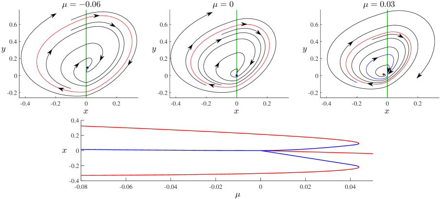
Figure 11.3: An illustration of HLB 20 for (11.23) with (11.24). By increasing the value of $\mu$ a stable node collides with the switching manifold when $\mu=0$ at which it turns into an unstable focus and emits a stable limit cycle. The limit cycle subsequently undergoes a saddle-node bifurcation and becomes unstable.

12 Discussion

In this paper we have detailed $20$ HLBs by which a steady-state solution can transition to sustained small amplitude oscillations in systems for which the equations of motion are piecewise-smooth. In most cases an isolated steady-state solution changes stability at $\mu=0$ and we identified a scalar quantity $\beta$ so that the steady-state solution is stable if $\beta\mu<0$ and unstable if $\beta\mu>0$. We identified a second scalar quantity $\alpha$ so that when $\mu=0$ the steady-state solution is stable if $\alpha<0$ and unstable if $\alpha>0$. If $\alpha<0$ and $\beta\mu>0$, then the competing effects of attraction and repulsion produce a stable limit cycle. With these inequalities reversed the limit cycle is unstable.

For each HLB we have provided formulas for $\beta$ and $\alpha$ in terms of the coefficients of a (sometimes piecewise) power series of the ODEs centred at $(x,y)=(0,0)$. For a Hopf bifurcation, $\beta$ is determined by linear terms in the series while $\alpha$ is determined by higher-order terms. The same is true for some HLBs, but for HLBs 1–6, 11–13, 15, 16 and 19, linear terms fully determine $\beta$ and $\alpha$. It is not surprising then that these HLBs produce a limit cycle whose amplitude is proportional to $|\mu|$, to leading order, see Table 1.1. In order to have square-root growth (like a Hopf bifurcation) the bifurcation must either involve a two-fold or have degenerate higher-order terms (as in ZoKu06 , for example).

Nonlinear terms influence the value of $\alpha$ for each of the other HLBs, although it is only for HLBs 8 and 19 that nonlinear terms are necessary to construct an instance of the bifurcation that is generic. For example, quartic terms affect the value of $\alpha$ for HLB 10, yet the piecewise-linear system (8.24) exhibits HLB 10 in a generic fashion.

Naturally we would like to extend the results to higher dimensions (i.e. systems with more than two variables). This is possible for the Hopf bifurcation theorem due to the presence of a two-dimensional centre manifold on which all the relevant dynamics occurs Ku04 . The majority of the HLBs presented here will not generate a centre manifold. For BEBs and other discontinuity induced bifurcations of piecewise-smooth systems the possible complexity of the local dynamics increases rapidly with dimension GlJe15 . This suggests that statements regarding limit cycles in higher dimensions will need to be weaker than those presented here. Attempts to make strong statements may lead to a proliferation of cases Gl17b (if $20$ HLBs are not enough already!). But certainly the basic geometric mechanisms described here for the creation of a limit cycle (e.g. BEBs, loss of stability, inclusion of delay) should be identifiable for higher dimensional systems, if only qualitatively.

Appendix A Derivations of the three return maps

Proof of Lemma 4.4.

Since $f$ and $g$ are $C^{2}$ they may be Taylor expanded to second order; we write

$$\begin{split}f(x,y)&=a_{1}x+a_{2}y+a_{3}x^{2}+a_{4}xy+a_{5}y^{2}+o\mathopen{}\mathclose{{}\left(\mathopen{}\mathclose{{}\left(|x|+|y|}\right)^{2}}\right),\\ g(x,y)&=b_{1}x+b_{2}y+b_{3}x^{2}+b_{4}xy+b_{5}y^{2}+o\mathopen{}\mathclose{{}\left(\mathopen{}\mathclose{{}\left(|x|+|y|}\right)^{2}}\right),\end{split}$$

which is consistent with (4.4). In order to expand asymptotically in $r$, we ‘blow up’ a neighbourhood of the origin via

$$\tilde{x} =\frac{x}{r}, \tilde{y} =\frac{y}{r},$$

where $r>0$. In these coordinates the system is given by

$$\begin{split}\dot{\tilde{x}}&=a_{1}\tilde{x}+a_{2}\tilde{y}+r\mathopen{}\mathclose{{}\left(a_{3}\tilde{x}^{2}+a_{4}\tilde{x}\tilde{y}+a_{5}\tilde{y}^{2}}\right)+o(r),\\ \dot{\tilde{y}}&=b_{1}\tilde{x}+b_{2}\tilde{y}+r\mathopen{}\mathclose{{}\left(b_{3}\tilde{x}^{2}+b_{4}\tilde{x}\tilde{y}+b_{5}\tilde{y}^{2}}\right)+o(r).\end{split}$$ (A.1)

We denote the $\tilde{x}$ and $\tilde{y}$ components of the flow of (A.1) by $\varphi_{t}(\tilde{x},\tilde{y})$ and $\psi_{t}(\tilde{x},\tilde{y})$, respectively. The trajectory associated with $P_{\rm focus}$ is the forward orbit of $(\tilde{x},\tilde{y})=(0,1)$. Thus $P_{\rm focus}$ and $T_{\rm focus}$ satisfy

$$\varphi_{T_{\rm focus}(r)}(0,1) =0,$$ (A.2)

$$\psi_{T_{\rm focus}(r)}(0,1) =\frac{1}{r}\,P_{\rm focus}(r).$$ (A.3)

Notice (A.1) is $C^{1}$ in $r$, thus $T_{\rm focus}(r)$ and $\frac{1}{r}P_{\rm focus}(r)$ are $C^{1}$ by Lemma 4.3, which justifies the error terms in (4.7)–(4.8).

The form (A.1) is a regular expansion in powers of $r$, thus the proof can be completed through direct asymptotic expansions in powers of $r$. We write

$$\begin{split}\varphi_{t}(0,1)&=\Phi^{(0)}_{t}(r)+r\Phi^{(1)}_{t}(r)+o(r),\\ \psi_{t}(0,1)&=\Psi^{(0)}_{t}(r)+r\Psi^{(1)}_{t}(r)+o(r),\end{split}$$

and by substituting these into (A.1) we obtain

$$\begin{split}\dot{\Phi}^{(0)}_{t}+r\dot{\Phi}^{(1)}_{t}&=a_{1}\mathopen{}\mathclose{{}\left(\Phi^{(0)}_{t}+r\Phi^{(1)}_{t}}\right)+a_{2}\mathopen{}\mathclose{{}\left(\Psi^{(0)}_{t}+r\Psi^{(1)}_{t}}\right)+r\mathopen{}\mathclose{{}\left(a_{3}\Phi^{(0)^{\scriptstyle 2}}_{t}+a_{4}\Phi^{(0)}_{t}\Psi^{(0)}_{t}+a_{5}\Psi^{(0)^{\scriptstyle 2}}_{t}}\right)+o(r),\\ \dot{\Psi}^{(0)}_{t}+r\dot{\Psi}^{(1)}_{t}&=b_{1}\mathopen{}\mathclose{{}\left(\Phi^{(0)}_{t}+r\Phi^{(1)}_{t}}\right)+b_{2}\mathopen{}\mathclose{{}\left(\Psi^{(0)}_{t}+r\Psi^{(1)}_{t}}\right)+r\mathopen{}\mathclose{{}\left(b_{3}\Phi^{(0)^{\scriptstyle 2}}_{t}+b_{4}\Phi^{(0)}_{t}\Psi^{(0)}_{t}+b_{5}\Psi^{(0)^{\scriptstyle 2}}_{t}}\right)+o(r),\end{split}$$ (A.4)

with initial condition

$$\begin{split}\Phi^{(0)}_{0}+r\Phi^{(1)}_{0}+o(r)&=0,\\ \Psi^{(0)}_{0}+r\Psi^{(1)}_{0}+o(r)&=1.\end{split}$$ (A.5)

To leading order

$$\begin{bmatrix}\dot{\Phi}^{(0)}_{t}\\ \dot{\Psi}^{(0)}_{t}\end{bmatrix} =A\begin{bmatrix}\Phi^{(0)}_{t}\\ \Psi^{(0)}_{t}\end{bmatrix}, \begin{bmatrix}\Phi^{(0)}_{0}\\ \Psi^{(0)}_{0}\end{bmatrix} =\begin{bmatrix}0\\ 1\end{bmatrix},$$

where $A$ is the Jacobian matrix (4.4). This has the solution

$$\begin{bmatrix}\Phi^{(0)}_{t}\\ \Psi^{(0)}_{t}\end{bmatrix}={\rm e}^{tA}\begin{bmatrix}0\\ 1\end{bmatrix}.$$ (A.6)

The $r$-terms in (A.4)–(A.5) give

$$\begin{bmatrix}\dot{\Phi}^{(1)}_{t}\\ \dot{\Psi}^{(1)}_{t}\end{bmatrix} =A\begin{bmatrix}\Phi^{(1)}_{t}\\ \Psi^{(1)}_{t}\end{bmatrix}+h(t), \begin{bmatrix}\Phi^{(1)}_{0}\\ \Psi^{(1)}_{0}\end{bmatrix} =\begin{bmatrix}0\\ 0\end{bmatrix},$$

where

$$h(t)=\begin{bmatrix}a_{3}\Phi^{(0)^{\scriptstyle 2}}_{t}+a_{4}\Phi^{(0)}_{t}\Psi^{(0)}_{t}+a_{5}\Psi^{(0)^{\scriptstyle 2}}_{t}\\ b_{3}\Phi^{(0)^{\scriptstyle 2}}_{t}+b_{4}\Phi^{(0)}_{t}\Psi^{(0)}_{t}+b_{5}\Psi^{(0)^{\scriptstyle 2}}_{t}\end{bmatrix}.$$ (A.7)

This has the solution

$$\begin{bmatrix}\Phi^{(1)}_{t}\\ \Psi^{(1)}_{t}\end{bmatrix}={\rm e}^{tA}\int_{0}^{t}{\rm e}^{-sA}\,h(s)\,ds.$$ (A.8)

We now calculate $T_{\rm focus}$. To this end we write

$$T_{\rm focus}(r)=T^{(0)}+rT^{(1)}+o(r),$$

By (A.6) we have $\Phi^{(0)}_{t}=\frac{a_{2}}{\omega}\,{\rm e}^{\lambda t}\sin(\omega t)$, where $\lambda\pm{\rm i}\omega$ are the eigenvalues of $A$ (4.3), and so

$$T^{(0)}=\frac{\pi}{\omega}.$$ (A.9)

This is sufficient to verify (4.8), but to verify (4.7) we require $T^{(1)}$. Equation (A.9) implies $\Phi^{(0)}_{T_{\rm focus}(r)}=-a_{2}{\rm e}^{\frac{\lambda\pi}{\omega}}T^{(1)}r+o(r)$, and so from the $r$-terms in (A.2) we obtain

$$T^{(1)}=\frac{1}{a_{2}}\,{\rm e}^{\frac{-\lambda\pi}{\omega}}\Phi^{(1)}_{\frac{\pi}{\omega}}.$$ (A.10)

Next we calculate $P_{\rm focus}$ which is determined by (A.3). We write

$$\frac{1}{r}\,P_{\rm focus}(r)=P^{(0)}+rP^{(1)}+o(r),$$ (A.11)

with which (A.3) is

$$\Psi^{(0)}_{T_{\rm focus}(r)}+r\Psi^{(1)}_{T_{\rm focus}(r)}=P^{(0)}+rP^{(1)}+o(r).$$ (A.12)

By (A.6) we have $\Psi^{(0)}_{t}={\rm e}^{\lambda t}\mathopen{}\mathclose{{}\left(\cos(\omega t)-\frac{a_{1}-b_{2}}{2\omega}\,\sin(\omega t)}\right)$, and so by (A.9) we obtain

$$P^{(0)}=-{\rm e}^{\frac{\lambda\pi}{\omega}}.$$ (A.13)

From the $r$-terms in (A.12) we obtain (after simplification using $\lambda=\frac{a_{1}+b_{2}}{2}$)

$$P^{(1)}=-\frac{b_{2}}{a_{2}}\,\Phi^{(1)}_{\frac{\pi}{\omega}}+\Psi^{(1)}_{\frac{\pi}{\omega}}.$$ (A.14)

To complete the proof it remains for us to evaluate (A.8) at $t=\frac{\pi}{\omega}$. Observe ${\rm e}^{\frac{\pi A}{\omega}}=-{\rm e}^{\frac{\lambda\pi}{\omega}}I$, thus

$$\begin{bmatrix}\Phi^{(1)}_{\frac{\pi}{\omega}}\\ \Psi^{(1)}_{\frac{\pi}{\omega}}\end{bmatrix}=-{\rm e}^{\frac{\lambda\pi}{\omega}}\int_{0}^{\frac{\pi}{\omega}}{\rm e}^{-sA}\,h(s)\,ds.$$ (A.15)

By the laborious task of expanding and grouping terms using (A.6) and (A.7), we obtain

$${\rm e}^{-sA}\,h(s)={\rm e}^{\lambda s}\begin{bmatrix}\sum\limits_{n=0}^{3}\frac{c_{n}}{\omega^{n}}\,\cos^{3-n}(\omega s)\sin^{n}(\omega s)\\ \sum\limits_{n=0}^{3}\frac{d_{n}}{\omega^{n}}\,\cos^{3-n}(\omega s)\sin^{n}(\omega s)\end{bmatrix},$$ (A.16)

where

$$\begin{split}c_{0}&=a_{5}\,,\\ c_{1}&=a_{2}(a_{4}-b_{5})-\frac{3(a_{1}-b_{2})a_{5}}{2},\\ c_{2}&=a_{2}^{2}(a_{3}-b_{4})-a_{2}(a_{1}-b_{2})(a_{4}-b_{5})+\frac{3a_{5}(a_{1}-b_{2})^{2}}{4},\\ c_{3}&=-a_{2}^{3}b_{3}-\frac{a_{2}^{2}(a_{1}-b_{2})(a_{3}-b_{4})}{2}\\ &\quad+\frac{a_{2}(a_{1}-b_{2})^{2}(a_{4}-b_{5})}{4}-\frac{a_{5}(a_{1}-b_{2})^{3}}{8},\\ d_{0}&=b_{5}\,,\\ d_{1}&=a_{2}b_{4}-a_{5}b_{1}-\frac{(a_{1}-b_{2})b_{5}}{2},\\ d_{2}&=a_{2}^{2}b_{3}-a_{2}a_{4}b_{1}+(a_{1}-b_{2})a_{5}b_{1}-\frac{(a_{1}-b_{2})^{2}b_{5}}{4},\\ d_{3}&=-a_{2}^{2}a_{3}b_{1}+\frac{a_{2}^{2}(a_{1}-b_{2})b_{3}}{2}+\frac{a_{2}(a_{1}-b_{2})a_{4}b_{1}}{2}\\ &\quad-\frac{a_{2}(a_{1}-b_{2})^{2}b_{4}}{4}-\frac{(a_{1}-b_{2})^{2}a_{5}b_{1}}{4}+\frac{(a_{1}-b_{2})^{3}b_{5}}{8}.\end{split}$$ (A.17)

Direct evaluation of

$$I_{n}=\int_{0}^{\frac{\pi}{\omega}}{\rm e}^{\lambda s}\cos^{3-n}(\omega s)\sin^{n}(\omega s)\,ds,$$ (A.18)

where $n=0,\ldots,3$, yields

$$I_{n}=\frac{\mathopen{}\mathclose{{}\left({\rm e}^{\frac{\lambda\pi}{\omega}}+1}\right)q_{n}}{\mathopen{}\mathclose{{}\left(\lambda^{2}+\omega^{2}}\right)\mathopen{}\mathclose{{}\left(\lambda^{2}+9\omega^{2}}\right)},$$ (A.19)

where

$$\begin{split}q_{0}&=-\lambda\mathopen{}\mathclose{{}\left(\lambda^{2}+7\omega^{2}}\right),\\ q_{1}&=\omega\mathopen{}\mathclose{{}\left(\lambda^{2}+3\omega^{2}}\right),\\ q_{2}&=-2\lambda\omega^{2},\\ q_{3}&=6\omega^{3}.\end{split}$$ (A.20)

Combining (A.14), (A.15), (A.16), (A.18), and (A.19) produces

$$P^{(1)}=\frac{{\rm e}^{\frac{\lambda\pi}{\omega}}\mathopen{}\mathclose{{}\left({\rm e}^{\frac{\lambda\pi}{\omega}}+1}\right)}{\mathopen{}\mathclose{{}\left(\lambda^{2}+\omega^{2}}\right)\mathopen{}\mathclose{{}\left(\lambda^{2}+9\omega^{2}}\right)}\sum_{n=0}^{3}\mathopen{}\mathclose{{}\left(\frac{b_{2}c_{n}}{a_{2}}-d_{n}}\right)\frac{q_{n}}{\omega^{n}}.$$

Finally from (A.17) and (A.20) we obtain

$$\sum_{n=0}^{3}\mathopen{}\mathclose{{}\left(\frac{b_{2}c_{n}}{a_{2}}-d_{n}}\right)\frac{q_{n}}{\omega^{n}} =2a_{3}k_{1}+a_{4}k_{2}+2a_{5}k_{3}$$

$$\quad+2b_{3}\ell_{1}+b_{4}\ell_{2}+2b_{5}\ell_{3}\,,$$

hence $P^{(1)}={\rm e}^{\frac{\lambda\pi}{\omega}}\mathopen{}\mathclose{{}\left({\rm e}^{\frac{\lambda\pi}{\omega}}+1}\right)\chi_{\rm focus}$, as required. ∎

Proof of Lemma 4.5.

Here we perform direct asymptotic expansions, but, for brevity, only include terms sufficient to obtain $P_{\rm fold}$ and $T_{\rm fold}$ to second order. One simply includes more terms to obtain (4.14) to fourth order.

We denote the $x$ and $y$ components of the flow by $\varphi_{t}(x,y)$ and $\psi_{t}(x,y)$, respectively. By substituting Taylor expansions for $\varphi_{t}(0,r)$ and $\psi_{t}(0,r)$ into the ODEs and matching terms using (4.11) we obtain

$$\varphi_{t}(0,r) =a_{2}rt+\frac{a_{2}b_{0}}{2}\,t^{2}+a_{5}r^{2}t$$

$$\quad+\mathopen{}\mathclose{{}\left(\frac{a_{1}a_{2}}{2}+\frac{a_{2}b_{2}}{2}+a_{5}b_{0}}\right)rt^{2}$$

$$\quad+\mathopen{}\mathclose{{}\left(\frac{a_{1}a_{2}b_{0}}{6}+\frac{a_{2}b_{0}b_{2}}{6}+\frac{a_{5}b_{0}^{2}}{3}}\right)t^{3}+O\mathopen{}\mathclose{{}\left((r+t)^{4}}\right),$$

$$\psi_{t}(0,r) =r+b_{0}t+b_{2}rt+\frac{b_{0}b_{2}}{2}\,t^{2}+O\mathopen{}\mathclose{{}\left((r+t)^{3}}\right).$$

We then solve $\varphi_{t}(0,r)=0$ for $t=T_{\rm fold}(r)$. Since $t=0$ is a solution to $\varphi_{t}(0,r)=0$, we use the IFT to solve $\frac{1}{t}\,\varphi_{t}(0,r)=0$. This is possible because $a_{2}b_{0}\neq 0$ and implies $T_{\rm fold}(r)$ is $C^{4}$ at $r=0$. By matching terms we obtain

$$T_{\rm fold}(r)=\frac{-2}{b_{0}}\,r+\frac{2\sigma_{\rm fold}}{3b_{0}}\,r^{2}+O\mathopen{}\mathclose{{}\left(r^{3}}\right),$$

where $\sigma_{\rm fold}$ is given by (4.12). Then

$$P_{\rm fold}(r) =\psi_{T_{\rm fold}}(0,r)$$

$$=-r+\frac{2\sigma_{\rm fold}}{3}\,r^{2}+O\mathopen{}\mathclose{{}\left(r^{3}}\right),$$

and has the same degree of differentiability at $r=0$ as $T_{\rm fold}$. ∎

Proof of Lemma 4.6.

First we derive (4.25)–(4.26). Since (4.17) is affine, it admits the analytical solution

$$\begin{bmatrix}\varphi_{t}(x,y)\\ \psi_{t}(x,y)\end{bmatrix}={\rm e}^{tA}\mathopen{}\mathclose{{}\left(\begin{bmatrix}x\\ y\end{bmatrix}-\begin{bmatrix}x^{*}\\ y^{*}\end{bmatrix}}\right)+\begin{bmatrix}x^{*}\\ y^{*}\end{bmatrix},$$ (A.21)

where

$${\rm e}^{tA}={\rm e}^{\lambda t}\begin{bmatrix}\cos(\omega t)+\frac{a_{1}-b_{2}}{2\omega}\,\sin(\omega t)&\frac{a_{2}}{\omega}\,\sin(\omega t)\\ \frac{b_{1}}{\omega}\,\sin(\omega t)&\cos(\omega t)-\frac{a_{1}-b_{2}}{2\omega}\,\sin(\omega t)\end{bmatrix},$$ (A.22)

and the equilibrium $(x^{*},y^{*})$ is given by (4.20). Also

$$\lambda =\frac{a_{1}+b_{2}}{2}, \omega =\sqrt{-a_{2}b_{1}-\frac{(a_{1}-b_{2})^{2}}{4}}.$$

Upon substituting $(x,y)=(0,r)$ into (A.21), we obtain, after much simplification,

$$\varphi_{t}(0,r) =\frac{a_{2}}{\omega}\,{\rm e}^{\lambda t}\sin(\omega t)r+\frac{a_{2}\kappa}{\omega}\,\varrho\mathopen{}\mathclose{{}\left(\omega t;\tfrac{\lambda}{\omega}}\right),$$ (A.23)

$$\psi_{t}(0,r) =\mathopen{}\mathclose{{}\left(\cos(\omega t)-\frac{a_{1}-b_{2}}{2\omega}\,\sin(\omega t)}\right)\mathopen{}\mathclose{{}\left({\rm e}^{\lambda t}r+\frac{\kappa\varrho\mathopen{}\mathclose{{}\left(\omega t;\frac{\lambda}{\omega}}\right)}{\sin(\omega t)}}\right)$$

$$\quad+\frac{\kappa{\rm e}^{\lambda t}\varrho\mathopen{}\mathclose{{}\left(\omega t;-\frac{\lambda}{\omega}}\right)}{\sin(\omega t)},$$ (A.24)

where $\kappa=\frac{b_{0}\omega}{\lambda^{2}+\omega^{2}}$, see (4.21), and $\varrho$ is the auxiliary function (4.22). The evolution time $T$ is defined by $\varphi_{T}(0,r)=0$, and through (A.23) we obtain (4.25). To evaluate $P=\psi_{T}(0,r)$, we substitute (4.25) into (A.24), with which the first part of (A.24) vanishes leaving (4.26).

Next we analyse the evolution time $T$. If $b_{0}<0$, then $x^{*}<0$, and so as the orbit travels from $(0,r)$ to $(0,P)$ it completes less than half a revolution around $(x^{*},y^{*})$, Fig. 4.6. The time taken to complete half a revolution is $\frac{\pi}{\omega}$, thus $\omega T\in(0,\pi)$ and $\sin(\omega T)>0$. If instead $b_{0}>0$, then $\omega T\in(\pi,2\pi)$ and $\sin(\omega T)<0$. By using the identity

$$\frac{\partial}{\partial s}\frac{{\rm e}^{-\nu s}\varrho(s;\nu)}{\sin(s)}=\frac{\varrho(s;-\nu)}{\sin^{2}(s)}$$ (A.25)

to differentiate (4.25), we obtain

$$\frac{dT}{dr}=-\frac{{\rm e}^{\lambda T}\sin(\omega T)}{\omega P}.$$ (A.26)

Since $\omega>0$ and $P<0$, we conclude that $\frac{dT}{dr}>0$ if $b_{0}<0$ (here $\sin(\omega T)>0$) and $\frac{dT}{dr}<0$ if $b_{0}>0$ (here $\sin(\omega T)<0$). Moreover by (4.25) we have $\lim_{r\to\infty}T=\frac{\pi}{\omega}$ (here $\sin(\omega T)\to 0$).

Now we analyse $P$. By (4.25)–(4.26), $\frac{P}{r}=\frac{-{\rm e}^{2\lambda T}\varrho\mathopen{}\mathclose{{}\left(\omega T;-\frac{\lambda}{\omega}}\right)}{\varrho\mathopen{}\mathclose{{}\left(\omega T;\frac{\lambda}{\omega}}\right)}$. Substituting $T=\frac{\pi}{\omega}$ gives $\frac{P}{r}=-{\rm e}^{\frac{\lambda\pi}{\omega}}$. Thus $P\sim-r\,{\rm e}^{\frac{\lambda\pi}{\omega}}$ as $r\to\infty$. By applying (A.25) to (4.25)–(4.26) we obtain

$$\frac{dP}{dr}=-\frac{\varrho\mathopen{}\mathclose{{}\left(\omega T;\frac{\lambda}{\omega}}\right)}{\varrho\mathopen{}\mathclose{{}\left(\omega T;-\frac{\lambda}{\omega}}\right)},$$ (A.27)

and a further application of (4.25)–(4.26) yields (4.27). This implies $\frac{dP}{dr}<0$ (because $r>0$ and $P<0$).

Finally we treat Types I–III in order.

1. By (4.25), as $r\to 0$, $\varrho\mathopen{}\mathclose{{}\left(\omega T;\frac{\lambda}{\omega}}\right)\to 0$. With $b_{0}<0$, $\omega T\in(0,\pi)$, so as $r\to 0$ we must have $T\to 0$ (see Fig. 4.5). Similarly $P\to 0$ by (4.26).

2. If $b_{0}>0$ and $\lambda<0$, then $\omega T\in(\pi,2\pi)$ and so by (4.26) and the definition of $\hat{s}$, see (4.24), we have $P=0$ when $T=\frac{\hat{s}(\nu)}{\omega}$, where $\nu=-\frac{\lambda}{\omega}>0$. To show that this occurs when $r=\hat{r}$, we substitute $T=\frac{\hat{s}(\nu)}{\omega}$ into (4.25) and use the identity

   $$\varrho(\hat{s}(\nu);-\nu)=\mathopen{}\mathclose{{}\left(1+\nu^{2}}\right)\sin^{2}(\hat{s}(\nu)),$$ (A.28)

   to obtain $r=-\kappa(1+\nu^{2})\,{\rm e}^{\nu\hat{s}(\nu)}\sin(\hat{s})=\hat{r}$. Since $P\in(-\infty,0)$ is a decreasing function of $r$, $P$ is undefined for all $r<\hat{r}$.

3. If $b_{0}>0$ and $\lambda>0$, again $\omega T\in(\pi,2\pi)$ and so by (4.25) we have $r=0$ when $T=\frac{\hat{s}(\nu)}{\omega}$, where $\nu=\frac{\lambda}{\omega}>0$. Here $P=\frac{b_{0}}{\omega}\,{\rm e}^{\nu\hat{s}(\nu)}\sin(\hat{s}(\nu))$ by (A.28).

∎

Appendix B Proofs for boundary equilibrium bifurcations

We start by proving the theorem for HLB 4. The theorem for HLB 1 is then a simple corollary. The proof for HLB 4 involves a blow-up of phase space about the origin so that the limit $\mu\to 0^{+}$ produces a piecewise-linear system for which a Poincaré map can be described using Lemma 4.6. The Poincaré map is shown to have a unique fixed point by generalising analytical arguments developed in FrPo98 . After this we prove the theorems for HLBs 2, 3 and 20.

Proof of Theorem 6.2 (HLB 4).

Write

$$\begin{split}f_{J}(x,y;\mu)&=a_{1J}x+a_{2J}y+a_{3J}\mu+O\mathopen{}\mathclose{{}\left(\mathopen{}\mathclose{{}\left(|x|+|y|+|\mu|}\right)^{2}}\right),\\ g_{J}(x,y;\mu)&=b_{1J}x+b_{2J}y+b_{3J}\mu+O\mathopen{}\mathclose{{}\left(\mathopen{}\mathclose{{}\left(|x|+|y|+|\mu|}\right)^{2}}\right),\end{split}$$ (B.1)

for each $J\in\{L,R\}$. Then

$$\beta_{J}=a_{3J}b_{2J}-a_{2J}b_{3J}\,,$$ (B.2)

and

$$\gamma=a_{2L}a_{3R}-a_{3L}a_{2R}\,.$$ (B.3)

In view of the replacement $y\mapsto-y$ it suffices to assume orbits rotate clockwise, that is $a_{2L}>0$ and $a_{2R}>0$.

Locally, the left half-system has a unique equilibrium: an unstable focus with $x$-value $\frac{-\beta_{L}\mu}{\lambda_{L}^{2}+\omega_{L}^{2}}+O\mathopen{}\mathclose{{}\left(\mu^{2}}\right)$. Since $\beta_{L}>0$, this equilibrium is admissible (in $\Omega_{L}$) for $\mu>0$. Similarly, locally, the right half-system has a unique equilibrium: a stable focus with $x$-value $\frac{-\beta_{R}\mu}{\lambda_{R}^{2}+\omega_{R}^{2}}+O\mathopen{}\mathclose{{}\left(\mu^{2}}\right)$. Since $\beta_{R}>0$, this equilibrium is admissible (in $\Omega_{R}$) for $\mu<0$.

For each $J\in\{L,R\}$, $f_{J}$ is $C^{2}$ and $a_{2J}\neq 0$ thus, by the IFT, $f_{J}(0,\zeta_{J}(\mu);\mu)=0$ for a unique $C^{2}$ function

$$\zeta_{J}(\mu)=-\frac{a_{3J}}{a_{2J}}\,\mu+O\mathopen{}\mathclose{{}\left(\mu^{2}}\right),$$ (B.4)

defined in a neighbourhood of $\mu=0$. The points $(0,\zeta_{L}(\mu))$ and $(0,\zeta_{R}(\mu))$ are folds, and observe

$$\zeta_{L}(\mu)-\zeta_{R}(\mu)=\frac{\gamma}{a_{2L}a_{2R}}\,\mu+O\mathopen{}\mathclose{{}\left(\mu^{2}}\right).$$ (B.5)

The folds may be classified by Definition 3.3 (recall $\beta_{L},\beta_{R}>0$). At $(0,\zeta_{L}(\mu))$, $\frac{\partial f_{L}}{\partial y}g_{L}=-\beta_{L}\mu+O\mathopen{}\mathclose{{}\left(\mu^{2}}\right)$, thus $(0,\zeta_{L}(\mu))$ is visible for $\mu>0$ [invisible for $\mu<0$]. Similarly at $(0,\zeta_{R}(\mu))$, $\frac{\partial f_{R}}{\partial y}g_{R}=-\beta_{R}\mu+O\mathopen{}\mathclose{{}\left(\mu^{2}}\right)$, thus $(0,\zeta_{R}(\mu))$ is invisible for $\mu>0$ [visible for $\mu<0$].

For the remainder of the proof we consider $\mu\geq 0$. This is because the result for $\mu<0$ follows from the following symmetry property: flipping the signs of $x$ and $\mu$ and reversing the direction of time transforms (6.1) to another system of this form satisfying the conditions of Theorem 6.2.

In order to accommodate the nonlinear terms in (B.1), we work in scaled coordinates

$$\tilde{x} =\frac{x}{\mu}, \tilde{y} =\frac{y-\zeta_{R}(\mu)}{\mu}.$$ (B.6)

This blow-up shifts the vertical coordinate to put the right fold at the origin. In these coordinates the right half-system is

$$\begin{split}\dot{\tilde{x}}&=a_{1R}\tilde{x}+a_{2R}\tilde{y}+O(\mu),\\ \dot{\tilde{y}}&=-\frac{\beta_{R}}{a_{2R}}+b_{1R}\tilde{x}+b_{2R}\tilde{y}+O(\mu),\end{split}$$ (B.7)

and the left half-system is

$$\begin{split}\dot{\tilde{x}}&=-\frac{\gamma}{a_{2R}}+a_{1L}\tilde{x}+a_{2L}\tilde{y}+O(\mu),\\ \dot{\tilde{y}}&=-\frac{a_{2R}b_{3L}-a_{3R}b_{2L}}{a_{2R}}+b_{1L}\tilde{x}+b_{2L}\tilde{y}+O(\mu).\end{split}$$ (B.8)

Fig. B.1 shows a phase portrait. Since $\gamma\geq 0$ by assumption, $\zeta_{L}(\mu)\geq\zeta_{R}(\mu)$ by (B.5).

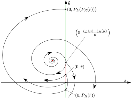
Figure B.1: For HLB 4, a sketch of the local dynamics with $\mu>0$ and using the coordinates (B.6). There exists an admissible unstable focus in $\Omega_{L}$; a visible fold of the left half-system and an invisible fold of the right half-system bound a repelling sliding region. On this region the direction of sliding motion is not indicated because there may be pseudo-equilibria, see Si18f .

Given $\tilde{r}>0$, consider the forward orbit of $(\tilde{x},\tilde{y})=(0,\tilde{r})$ that immediately enters $\tilde{x}>0$. Let $P_{R}(\tilde{r};\mu)$ be the $\tilde{y}$-value of the next intersection of this orbit with $\tilde{x}=0$ (leave $P_{R}$ undefined if this orbit does not return to $\tilde{x}=0$) and let $T_{R}(\tilde{r};\mu)$ be the corresponding evolution time. Similarly for any $\tilde{r}<0$, let $P_{L}(\tilde{r};\mu)$ be the $\tilde{y}$-value of the next intersection of the forward orbit of $(0,\tilde{r})$ with $\tilde{x}=0$ (leave $P_{L}$ undefined if this orbit does not return to $\tilde{x}=0$) and let $T_{L}(\tilde{r};\mu)$ be the corresponding evolution time. Let

$$P(\tilde{r};\mu)=P_{L}\mathopen{}\mathclose{{}\left(P_{R}(\tilde{r};\mu);\mu}\right),$$ (B.9)

be the induced Poincaré map. This corresponds to an evolution time of

$$T(\tilde{r};\mu)=T_{R}(\tilde{r};\mu)+T_{L}\mathopen{}\mathclose{{}\left(P_{R}(\tilde{r};\mu);\mu}\right).$$ (B.10)

Fixed points of $P$ correspond to periodic orbits of (B.7)–(B.8) and thus also of the original system (6.1). Locally, periodic orbits of (6.1) must evolve on both sides of $x=0$, thus the fixed points of $P$ generate all local periodic orbits of (6.1).

Although the scaled system (B.7)–(B.8) was constructed under the assumption $\mu>0$, in (B.7)–(B.8) we may set $\mu=0$. Next we analyse $P$ and $T$ with $\mu=0$ and accommodate $\mu>0$ at the end.

With $\mu=0$, (B.7) is affine and we can apply Lemma 4.6 with $b_{0}=-\frac{\beta_{R}}{a_{2R}}$. Specifically,

$$\begin{split}P_{R}(\tilde{r};0)&=P_{\rm affine}\mathopen{}\mathclose{{}\left(\tilde{r};\lambda_{R},\omega_{R},-\tfrac{\beta_{R}}{a_{2R}}}\right),\\ T_{R}(\tilde{r};0)&=T_{\rm affine}\mathopen{}\mathclose{{}\left(\tilde{r};\lambda_{R},\omega_{R},-\tfrac{\beta_{R}}{a_{2R}}}\right),\end{split}$$ (B.11)

which are of Type I because $b_{0}<0$. In order to apply Lemma 4.6 to (B.7), we rotate coordinates by $180^{\circ}$ and translate so that the fold is at the origin. Specifically, we let

$$\begin{split}\tilde{\tilde{x}}&=-\tilde{x},\\ \tilde{\tilde{y}}&=-\mathopen{}\mathclose{{}\left(\tilde{y}-\tilde{\gamma}}\right),\end{split}$$ (B.12)

where

$$\tilde{\gamma}=\frac{\gamma}{a_{2L}a_{2R}},$$ (B.13)

with which (B.8) with $\mu=0$ becomes

$$\begin{split}\dot{\tilde{\tilde{x}}}&=a_{1L}\tilde{\tilde{x}}+a_{2L}\tilde{\tilde{y}},\\ \dot{\tilde{\tilde{y}}}&=\frac{\beta_{L}}{a_{2L}}+b_{1L}\tilde{\tilde{x}}+b_{2L}\tilde{\tilde{y}}.\end{split}$$ (B.14)

Then Lemma 4.6 with $b_{0}=\frac{\beta_{L}}{a_{2L}}$ gives

$$\begin{split}P_{L}(\tilde{r};0)&=\tilde{\gamma}-P_{\rm affine}\mathopen{}\mathclose{{}\left(\tilde{\gamma}-\tilde{r};\lambda_{L},\omega_{L},\frac{\beta_{L}}{a_{2L}}}\right),\\ T_{L}(\tilde{r};0)&=T_{\rm affine}\mathopen{}\mathclose{{}\left(\tilde{\gamma}-\tilde{r};\lambda_{L},\omega_{L},\frac{\beta_{L}}{a_{2L}}}\right),\end{split}$$ (B.15)

which are of Type III because $b_{0}>0$ and $\lambda_{L}>0$. Notice $P(\tilde{r};0)$ is well-defined for all $\tilde{r}>0$.

By Lemma 4.6, $P_{R}(\tilde{r};0)\sim-\tilde{r}\,{\rm e}^{\frac{\lambda_{R}\pi}{\omega_{R}}}$ as $\tilde{r}\to\infty$, and $P_{L}(\tilde{r};0)\sim-\tilde{r}\,{\rm e}^{\frac{\lambda_{L}\pi}{\omega_{L}}}$ as $\tilde{r}\to-\infty$. Thus

$$P(\tilde{r};0)\sim\tilde{r}\,{\rm e}^{\alpha\pi},$$ (B.16)

as $\tilde{r}\to\infty$, where $\alpha=\frac{\lambda_{L}}{\omega_{L}}+\frac{\lambda_{R}}{\omega_{R}}$, (6.15). By (4.27) we obtain

$$\frac{\partial P}{\partial\tilde{r}}(\tilde{r};0)=\frac{\tilde{r}\mathopen{}\mathclose{{}\left(\tilde{\gamma}-P_{R}}\right)}{P_{R}\mathopen{}\mathclose{{}\left(\tilde{\gamma}-P}\right)}\,{\rm e}^{2h(\tilde{r})},$$ (B.17)

where

$$h(\tilde{r})=\lambda_{R}T_{R}(\tilde{r};0)+\lambda_{L}T_{L}\mathopen{}\mathclose{{}\left(P_{R}(\tilde{r};0);0}\right).$$ (B.18)

Observe $\tilde{r}>0$, and $P_{R}<0<\tilde{\gamma}<P$. For all $\tilde{r}>0$,

$$\frac{dh}{d\tilde{r}}<0,$$ (B.19)

because $\lambda_{R}<0$ and $T_{R}(\tilde{r};0)$ is increasing and $\lambda_{L}>0$ and $T_{L}\mathopen{}\mathclose{{}\left(P_{R}(\tilde{r};0);0}\right)$ is decreasing. The period of the limit cycle corresponding to a fixed point $\tilde{r}^{*}$ is $T=T_{L}+T_{R}$, where $P_{L}=\tilde{r}^{*}$, $P_{R}$, $T_{L}$, and $T_{R}$ satisfy

$$\tilde{r}^{*} =\frac{-\kappa_{R}\,{\rm e}^{-\lambda_{R}T_{R}}\varrho\big{(}\omega_{R}T_{R};\frac{\lambda_{R}}{\omega_{R}}\big{)}}{\sin(\omega_{R}T_{R})},$$

$$P_{R} =\frac{\kappa_{R}\,{\rm e}^{\lambda_{R}T_{R}}\varrho\big{(}\omega_{R}T_{R};-\frac{\lambda_{R}}{\omega_{R}}\big{)}}{\sin(\omega_{R}T_{R})},$$

$$\tilde{\gamma}-P_{R} =\frac{-\kappa_{L}\,{\rm e}^{-\lambda_{L}T_{L}}\varrho\big{(}\omega_{L}T_{L};\frac{\lambda_{L}}{\omega_{L}}\big{)}}{\sin(\omega_{L}T_{L})},$$

$$\tilde{\gamma}-P_{L} =\frac{\kappa_{L}\,{\rm e}^{\lambda_{L}T_{L}}\varrho\big{(}\omega_{L}T_{L};-\frac{\lambda_{L}}{\omega_{L}}\big{)}}{\sin(\omega_{L}T_{L})},$$

where $\kappa_{R}=\frac{-\beta_{R}\omega_{R}}{a_{2R}\mathopen{}\mathclose{{}\left(\lambda_{R}^{2}+\omega_{R}^{2}}\right)}$ and $\kappa_{L}=\frac{\beta_{L}\omega_{L}}{a_{2L}\mathopen{}\mathclose{{}\left(\lambda_{L}^{2}+\omega_{L}^{2}}\right)}$. By eliminating $P_{L}$ and $P_{R}$ in these equations we produce (6.18).

This completes our construction and basic description of the Poincaré map $P$ and the evolution time $T$. We now use a series of analytical arguments to characterise fixed points of $P$ in the limit $\mu\to 0^{+}$. Following the logical steps of FrPo98 , we suppose, for the moment, that $P(\tilde{r};0)$ has a fixed point, and let $\tilde{r}^{*}$ be the smallest such point. Since $P(0;0)>0$, we must have $P(\tilde{r};0)>\tilde{r}$, for all $0\leq\tilde{r}<\tilde{r}^{*}$, and so $\frac{\partial P}{\partial\tilde{r}}\mathopen{}\mathclose{{}\left(\tilde{r}^{*};0}\right)\leq 1$.

Now suppose, for a contradiction, that $\frac{\partial P}{\partial\tilde{r}}\mathopen{}\mathclose{{}\left(\tilde{r}^{*};0}\right)=1$. Then we need $\frac{\partial^{2}P}{\partial\tilde{r}^{2}}\mathopen{}\mathclose{{}\left(\tilde{r}^{*};0}\right)\geq 0$, because $P(\tilde{r};0)>\tilde{r}$ for all $0\leq\tilde{r}<\tilde{r}^{*}$. But by differentiating (B.17) and substituting $\tilde{r}=P=\tilde{r}^{*}$ and $\frac{\partial P}{\partial\tilde{r}}=1$, we get

$$\frac{\partial^{2}P}{\partial\tilde{r}^{2}}\mathopen{}\mathclose{{}\left(\tilde{r}^{*};0}\right)=\frac{\tilde{\gamma}}{\tilde{r}^{*}\mathopen{}\mathclose{{}\left(\tilde{\gamma}-\tilde{r}^{*}}\right)}-\frac{\tilde{\gamma}\,\frac{\partial P_{R}}{\partial\tilde{r}}}{P_{R}\mathopen{}\mathclose{{}\left(\tilde{\gamma}-P_{R}}\right)}+2\frac{dh}{d\tilde{r}}.$$ (B.20)

The first two terms (B.20) are non-positive, and the last term is negative, thus $\frac{\partial^{2}P}{\partial\tilde{r}^{2}}\mathopen{}\mathclose{{}\left(\tilde{r}^{*};0}\right)<0$, which is a contradiction. Hence $\frac{\partial P}{\partial\tilde{r}}\mathopen{}\mathclose{{}\left(\tilde{r}^{*};0}\right)<1$, and so $\tilde{r}^{*}$ is an asymptotically stable fixed point of $P(\tilde{r};0)$.

Next suppose, for a contradiction, that $P(\tilde{r};0)$ has other fixed points, and let $\tilde{r}^{**}$ be the next smallest such point. Then $P(\tilde{r};0)<\tilde{r}$ for all $\tilde{r}^{*}\leq\tilde{r}<\tilde{r}^{**}$ and so $\frac{\partial P}{\partial\tilde{r}}\mathopen{}\mathclose{{}\left(\tilde{r}^{**};0}\right)\geq 1$. At a fixed point, equation (B.17) is satisfied with $P=\tilde{r}$, that is

$$\frac{\partial P}{\partial\tilde{r}}(\tilde{r};0)=G(\tilde{r})\,{\rm e}^{2h(\tilde{r})},$$ (B.21)

where

$$G(\tilde{r})=\frac{\tilde{r}\mathopen{}\mathclose{{}\left(\tilde{\gamma}-P_{R}}\right)}{P_{R}\mathopen{}\mathclose{{}\left(\tilde{\gamma}-\tilde{r}}\right)}.$$

We have

$$\frac{dG}{d\tilde{r}}=\mathopen{}\mathclose{{}\left(\frac{\tilde{\gamma}}{\tilde{r}^{*}\mathopen{}\mathclose{{}\left(\tilde{\gamma}-\tilde{r}^{*}}\right)}-\frac{\tilde{\gamma}\,\frac{\partial P_{R}}{\partial\tilde{r}}}{P_{R}\mathopen{}\mathclose{{}\left(\tilde{\gamma}-P_{R}}\right)}}\right)G(\tilde{r}),$$

so $G$ is a decreasing function because $G$ is positive and, as above, the term in large brackets is negative. Since $h$ is decreasing, we conclude from (B.21) that $\frac{\partial P}{\partial\tilde{r}}(\tilde{r};0)$ is decreasing. But $\frac{\partial P}{\partial\tilde{r}}\mathopen{}\mathclose{{}\left(\tilde{r}^{*};0}\right)<1$, so we cannot have $\frac{\partial P}{\partial\tilde{r}}\mathopen{}\mathclose{{}\left(\tilde{r}^{**};0}\right)\geq 1$. This is contradiction, hence $P(\tilde{r};0)<\tilde{r}$ for all $\tilde{r}>\tilde{r}^{*}$.

By (B.16), this requires $\alpha\leq 0$. Thus $P(\tilde{r};0)$ has no fixed points if $\alpha>0$. If $\alpha<0$, then $P(\tilde{r};0)$ has a fixed point by the intermediate value theorem, and, as we have just shown, this fixed point is unique, call it $\tilde{r}^{*}$. Moreover, as shown above, $\frac{\partial P}{\partial\tilde{r}}\mathopen{}\mathclose{{}\left(\tilde{r}^{*};0}\right)<1$, thus the fixed point is asymptotically stable.

Finally we consider $P(\tilde{r};\mu)$ with $\mu>0$. Notice (B.7) and (B.8) are $C^{1}$ (with respect to both the variables $\tilde{x}$ and $\tilde{y}$ and the parameter $\mu$). Thus the flow of (B.7) and (B.8) are $C^{1}$ functions of the initial condition and of $\mu$. For all $\tilde{r}>0$, $P(\tilde{r};0)$ is well-defined and corresponds to transversal intersections with $\tilde{x}=0$, thus $P(\tilde{r};\mu)$ is well-defined and $C^{1}$, by Lemma 4.3, for sufficiently small $\mu>0$. By the IFT applied to $P$, if $\alpha<0$ then $P$ has a unique stable fixed point $\tilde{r}^{*}(\mu)$. Hence, locally, the scaled system (B.7)–(B.8) has a unique stable limit cycle, and the same is true for the original system (6.1). In view of (B.6), in (6.1) the size of the limit cycle is asymptotically proportional to $\mu$ (for example if $\tilde{x}_{\rm max}$ denotes the maximum $\tilde{x}$-value of the limit cycle in (B.7)–(B.8) with $\mu=0$, then the maximum $x$-value of the limit cycle in (6.1) is $\mu\tilde{x}_{\rm max}+O\mathopen{}\mathclose{{}\left(\mu^{2}}\right)$). If instead $\alpha>0$, then, locally, $P$ has no fixed points and thus (6.1) has no limit cycles. As mentioned above, the dynamics for $\mu<0$ follows by symmetry. ∎

Proof of Theorem 5.1 (HLB 1).

Unlike for Theorem 6.2, locally there must exist a unique stationary solution because (5.1) is continuous; the only stationary solutions are regular equilibria. The left half-system has an unstable focus with $x$-value $\frac{-\beta\mu}{\lambda_{L}^{2}+\omega_{L}^{2}}+O\mathopen{}\mathclose{{}\left(\mu^{2}}\right)$, so is admissible (in $\Omega_{L}$) for $\mu>0$ because $\beta>0$. Similarly the right half-system has admissible stable focus for $\mu<0$.

To complete the proof we apply Theorem 6.2. In (6.16) we have $\beta_{L}=\beta_{R}=\beta>0$. In (6.17) we have $\gamma=0$. Also $a_{2L}a_{2R}=\mathopen{}\mathclose{{}\left(\frac{\partial f_{L}}{\partial y}(0,0;0)}\right)^{2}$ is non-zero (and hence positive) because ${\rm D}F_{L}(0,0;0)$ has complex eigenvalues. This shows that the conditions of Theorem 6.2 are satisfied. The conclusions of Theorem 6.2 reduce to those Theorem 5.1; this completes the proof. ∎

Proof of Theorem 5.2 (HLB 2).

This proof follows that of Theorem 6.2 (given above) except we need to accommodate the real eigenvalues of the stable node and carefully consider the case $\mu<0$ (to show that no limit cycle exists when the node is admissible). Write

$$\begin{split}f_{J}(x,y;\mu)&=a_{1J}x+a_{2}y+a_{3}\mu+O\mathopen{}\mathclose{{}\left(\mathopen{}\mathclose{{}\left(|x|+|y|+|\mu|}\right)^{2}}\right),\\ g_{J}(x,y;\mu)&=b_{1J}x+b_{2}y+b_{3}\mu+O\mathopen{}\mathclose{{}\left(\mathopen{}\mathclose{{}\left(|x|+|y|+|\mu|}\right)^{2}}\right),\end{split}$$ (B.22)

for each $J\in\{L,R\}$. Notice $a_{2}\neq 0$ by the eigenvalue condition (5.11) and we can assume $a_{2}>0$ in view of the replacement $y\mapsto-y$. Also by (5.11), locally the left half-system has a unique equilibrium: an unstable focus with $x$-value $\frac{-\beta\mu}{\lambda_{L}^{2}+\omega_{L}^{2}}+O\mathopen{}\mathclose{{}\left(\mu^{2}}\right)$, that is admissible (in $\Omega_{L}$) for $\mu>0$ (because $\beta>0$). Similarly, locally, the right half-system has a unique equilibrium: a stable node with $x$-value $\frac{-\beta\mu}{\lambda_{R}^{2}-\eta_{R}^{2}}+O\mathopen{}\mathclose{{}\left(\mu^{2}}\right)$, that is admissible (in $\Omega_{R}$) for $\mu<0$. Since $f_{L}$ is $C^{2}$ and $a_{2}\neq 0$, by the IFT we have $f_{L}(0,\zeta(\mu);\mu)=0$ for a unique $C^{2}$ function

$$\zeta(\mu)=-\frac{a_{3}}{a_{2}}\,\mu+O\mathopen{}\mathclose{{}\left(\mu^{2}}\right),$$

defined in a neighbourhood of $\mu=0$. Notice $(x,y)=(0,\zeta(\mu))$ is a fold for both half-systems of (5.1).

First consider $\mu>0$. We introduce the scaled coordinates

$$\tilde{x} =\frac{x}{\mu}, \tilde{y} =\frac{y-\zeta(\mu)}{\mu},$$ (B.23)

with which the system becomes

$$\begin{split}\dot{\tilde{x}}&=a_{1J}\tilde{x}+a_{2}\tilde{y}+O(\mu),\\ \dot{\tilde{y}}&=-\frac{\beta}{a_{2}}+b_{1J}\tilde{x}+b_{2}\tilde{y}+O(\mu),\end{split}$$ (B.24)

with $J=L$ for $\tilde{x}<0$ and $J=R$ for $\tilde{x}>0$. Given $\tilde{r}>0$, let $P_{R}(\tilde{r};\mu)<0$ be the $\tilde{y}$-value of the next intersection of the forward orbit of $(0,\tilde{r})$ with $\tilde{x}=0$, and let $T_{R}(\tilde{r};\mu)$ be the corresponding evolution time. Similarly given $\tilde{r}<0$, let $P_{L}(\tilde{r};\mu)>0$ be the $\tilde{y}$-value of the next intersection of the forward orbit of $(0,\tilde{r})$ with $\tilde{x}=0$, and let $T_{L}(\tilde{r};\mu)$ be the corresponding evolution time. Let

$$P(\tilde{r};\mu)=P_{L}\mathopen{}\mathclose{{}\left(P_{R}(\tilde{r};\mu);\mu}\right),$$ (B.25)

which corresponds to an evolution time of

$$T(\tilde{r};\mu)=T_{R}(\tilde{r};\mu)+T_{L}\mathopen{}\mathclose{{}\left(P_{R}(\tilde{r};\mu);\mu}\right).$$ (B.26)

Locally, limit cycles must enter both $\tilde{x}<0$ and $\tilde{x}>0$, thus all possible limit cycles are generated by the fixed points of $P$.

Next we analyse $P(\tilde{r};0)$ and $T(\tilde{r};0)$ (which are well-defined even though (B.24) was constructed under the assumption $\mu>0$). In the limit $\mu\to 0^{+}$, (B.24) has the affine form (4.17). Thus for (B.24) with $J=R$,

$$\begin{split}P_{R}(\tilde{r};0)&=P_{\rm affine}\mathopen{}\mathclose{{}\left(\tilde{r};\lambda_{R},{\rm i}\eta_{R},-\frac{\beta}{a_{2}}}\right),\\ T_{R}(\tilde{r};0)&=T_{\rm affine}\mathopen{}\mathclose{{}\left(\tilde{r};\lambda_{R},{\rm i}\eta_{R},-\frac{\beta}{a_{2}}}\right),\end{split}$$

where the imaginary argument arises from putting the real eigenvalues $\lambda_{R}\pm\eta_{R}$ (5.11) in the complex form (4.19). Let

$$\varrho_{\rm node}(s;\nu)=1-{\rm e}^{\nu s}\mathopen{}\mathclose{{}\left(\cosh(s)-\nu\sinh(s)}\right).$$ (B.27)

Like $\varrho$ (see Fig. 4.5), the function $\varrho_{\rm node}$ has a double zero at $s=0$, but if $|\nu|>1$ then $\varrho_{\rm node}(s;\nu)>0$ for all $s\neq 0$. Using the identity $\varrho({\rm i}s;-{\rm i}\nu)=\varrho_{\rm node}(s;\nu)$, by Lemma 4.6

$$\tilde{r} =\frac{-{\rm Im}(\kappa_{R})\,{\rm e}^{-\lambda_{R}T_{R}}\varrho_{\rm node}\mathopen{}\mathclose{{}\left(\eta_{R}T_{R};\frac{\lambda_{R}}{\eta_{R}}}\right)}{\sinh\mathopen{}\mathclose{{}\left(\eta_{R}T_{R}}\right)},$$ (B.28)

$$P_{R} =\frac{{\rm Im}(\kappa_{R})\,{\rm e}^{\lambda_{R}T_{R}}\varrho_{\rm node}\mathopen{}\mathclose{{}\left(\eta_{R}T_{R};\frac{-\lambda_{R}}{\eta_{R}}}\right)}{\sinh\mathopen{}\mathclose{{}\left(\eta_{R}T_{R}}\right)},$$ (B.29)

where

$$\kappa_{R}=\frac{-{\rm i}\beta\eta_{R}}{a_{2}\mathopen{}\mathclose{{}\left(\lambda_{R}^{2}-\eta_{R}^{2}}\right)}.$$ (B.30)

Analogous to (A.26),

$$\frac{\partial T_{R}}{\partial\tilde{r}}=-\frac{{\rm e}^{\lambda_{R}T_{R}}\sinh(\eta_{R}T_{R})}{\eta_{R}P_{R}},$$ (B.31)

thus $T_{R}(\tilde{r};0)$ is an increasing function of $\tilde{r}$ (because $\eta_{R}>0$ and $P_{R}<0$). Analogous to (A.27),

$$\frac{\partial P_{R}}{\partial\tilde{r}}=-\frac{\varrho_{\rm node}\mathopen{}\mathclose{{}\left(\eta_{R}T_{R};\frac{\lambda_{R}}{\eta_{R}}}\right)}{\varrho_{\rm node}\mathopen{}\mathclose{{}\left(\eta_{R}T_{R};-\frac{\lambda_{R}}{\eta_{R}}}\right)},$$ (B.32)

thus $P_{R}(\tilde{r};0)$ is a decreasing function of $\tilde{r}$ (because $\big{|}\frac{\lambda_{R}}{\eta_{R}}\big{|}>1$). By (B.28)–(B.29), $T_{R}(\tilde{r};0)\to 0$ and $P_{R}(\tilde{r};0)\to 0$ as $\tilde{r}\to 0$. As $\tilde{r}\to\infty$,

$$\tilde{r}\sim-2{\rm Im}(\kappa_{R})\,{\rm e}^{-(\lambda_{R}+\eta_{R})T_{R}},$$ (B.33)

and

$$P_{R}(\tilde{r};0)\to\frac{-\beta}{a_{2}\mathopen{}\mathclose{{}\left(\eta_{R}-\lambda_{R}}\right)}.$$ (B.34)

Lemma 4.6 can be applied to (B.24) with $J=L$ (still in the limit $\mu\to 0^{+}$) by rotating coordinates by $180^{\circ}$. In this way we obtain

$$\begin{split}P_{L}(\tilde{r};0)&=-P_{\rm affine}\mathopen{}\mathclose{{}\left(-\tilde{r};\lambda_{L},\omega_{L},\frac{\beta}{a_{2}}}\right),\\ T_{L}(\tilde{r};0)&=T_{\rm affine}\mathopen{}\mathclose{{}\left(-\tilde{r};\lambda_{L},\omega_{L},\frac{\beta}{a_{2}}}\right),\end{split}$$ (B.35)

which are of Type III because $\frac{\beta}{a_{2}}>0$ and $\lambda_{L}>0$. It follows that $P(\tilde{r};0)=P_{L}\mathopen{}\mathclose{{}\left(P_{R}(\tilde{r};0);0}\right)$ is an increasing function of $\tilde{r}$ with $\lim_{\tilde{r}\to 0}P(\tilde{r};0)>0$ and $\lim_{\tilde{r}\to\infty}P(\tilde{r};0)<\infty$. By the intermediate value theorem, $P(\tilde{r};0)$ has a fixed point $\tilde{r}^{*}$. It can be shown that $\tilde{r}^{*}$ is asymptotically stable and unique (we omit this step for brevity; it can be achieved by a minor adaptation of arguments that appear in the proof of Theorem 6.2). Also by repeating the arguments at the end of the proof of Theorem 6.2 we conclude that $P(\tilde{r};\mu)$ has a unique stable fixed point $\tilde{r}^{*}(\mu)$ for sufficiently small $\mu>0$ because (B.24) is $C^{1}$. Thus (5.1) has a unique stable limit cycle with amplitude proportional to $\mu$ (due to the scaling (B.23)).

Second consider $\mu<0$. Let $\tilde{x}=\frac{x}{|\mu|}$ and $\tilde{y}=\frac{y-\zeta(\mu)}{|\mu|}$ and take $\mu\to 0^{-}$ with which the right half-system is affine with an admissible stable node $\mathopen{}\mathclose{{}\left(\tilde{x}_{R}^{*},\tilde{y}_{R}^{*}}\right)$, see Fig. B.2. Let $\ell_{1}$ be the line segment connecting $(0,0)$ and $\mathopen{}\mathclose{{}\left(\tilde{x}_{R}^{*},\tilde{y}_{R}^{*}}\right)$. Let $\ell_{2}$ be the linear slow subspace with $\tilde{x}\geq\tilde{x}_{R}^{*}$ (this has slope $\frac{\lambda_{R}+\eta_{R}-a_{1R}}{a_{2}}$). For all $\tilde{r}>0$, the forward orbit of $(0,\tilde{r})$ cannot cross $\ell_{1}$ (here $\dot{\tilde{x}}=0$ and $\dot{\tilde{y}}>0$) or $\ell_{2}$ (because $\ell_{2}$ is an invariant). Thus the orbit converges to $\mathopen{}\mathclose{{}\left(\tilde{x}_{R}^{*},\tilde{y}_{R}^{*}}\right)$ without reintersecting $\tilde{x}=0$. Now choose any $\tilde{r}_{\rm max}>0$. Since (B.24) is $C^{1}$ there exists $\delta>0$ such that for all $-\delta<\mu<0$, $\mathopen{}\mathclose{{}\left(\tilde{x}_{R}^{*},\tilde{y}_{R}^{*}}\right)$ persists as a stable node $\mathopen{}\mathclose{{}\left(\tilde{x}_{R}^{*}(\mu),\tilde{y}_{R}^{*}(\mu)}\right)$, and for all $0<\tilde{r}<\tilde{r}_{\rm max}$ the forward orbit of $(0,\tilde{r})$ converges to $\mathopen{}\mathclose{{}\left(\tilde{x}_{R}^{*}(\mu),\tilde{y}_{R}^{*}(\mu)}\right)$ without reintersecting $\tilde{x}=0$. Thus, locally, (B.24), and hence also (5.1), has no limit cycle for $\mu<0$. ∎

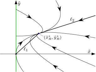
Figure B.2: For HLB 2, a sketch of the local dynamics with $\mu<0$ in scaled coordinates indicating the line segment $\ell_{1}$ and the ray $\ell_{2}$ defined in the text.

Proof of Theorem 6.1 (HLB 3).

Write

$$\begin{split}f_{L}(x,y;\mu)&=a_{1L}x+a_{2L}y+a_{3L}\mu+O\mathopen{}\mathclose{{}\left(\mathopen{}\mathclose{{}\left(|x|+|y|+|\mu|}\right)^{2}}\right),\\ g_{L}(x,y;\mu)&=b_{1L}x+b_{2L}y+b_{3L}\mu+O\mathopen{}\mathclose{{}\left(\mathopen{}\mathclose{{}\left(|x|+|y|+|\mu|}\right)^{2}}\right).\end{split}$$ (B.36)

Then

$$\beta =a_{3L}b_{2L}-a_{2L}b_{3L}\,,$$ (B.37)

$$\gamma =a_{2L}b_{0R}-a_{0R}b_{2L}\,,$$ (B.38)

where $b_{0R}=g_{R}(0,0;0)$. Notice $a_{2L}\neq 0$ by (6.4), and it suffices to assume $a_{2L}>0$ in view of the replacement $y\mapsto-y$. Locally the left half-system has a unique equilibrium: an unstable focus $\mathopen{}\mathclose{{}\left(x_{L}^{*}(\mu),y_{L}^{*}(\mu)}\right)$ with $x_{L}^{*}(\mu)=\frac{-\beta\mu}{\lambda_{L}^{2}+\omega_{L}^{2}}+O\mathopen{}\mathclose{{}\left(\mu^{2}}\right)$. Since $\beta>0$ the equilibrium is admissible (in $\Omega_{L}$) for $\mu>0$.

Since $f_{L}$ is $C^{2}$ and $a_{2L}\neq 0$, by the IFT we have $f_{L}(0,\zeta_{L}(\mu);\mu)=0$ for a unique $C^{2}$ function

$$\zeta_{L}(\mu)=-\frac{a_{3L}}{a_{2L}}\,\mu+O\mathopen{}\mathclose{{}\left(\mu^{2}}\right),$$ (B.39)

defined in a neighbourhood of $\mu=0$. Since $a_{2L}>0$ and $a_{0R}<0$, locally $x=0$ is a crossing region for $y<\zeta_{L}(\mu)$ and an attracting sliding region for $y>\zeta_{L}(\mu)$. On the attracting sliding region orbits evolve according to $\dot{y}=g_{\rm slide}(y;\mu)$, where $g_{\rm slide}$ is given by (3.7). Here

$$g_{\rm slide}(y;\mu)=\frac{-\gamma}{a_{0R}}\mathopen{}\mathclose{{}\left(y-\zeta_{L}(\mu)}\right)-\frac{\beta}{a_{2L}}\,\mu+O\mathopen{}\mathclose{{}\left(\mathopen{}\mathclose{{}\left(|y|+|\mu|}\right)^{2}}\right).$$ (B.40)

Pseudo-equilibria satisfy $g_{\rm slide}(y;\mu)=0$. Since (B.40) is $C^{2}$ and $\gamma\neq 0$, by the IFT there exists a unique pseudo-equilibrium $\mathopen{}\mathclose{{}\left(0,y_{\rm ps}^{*}(\mu)}\right)$ where $y_{\rm ps}^{*}(\mu)=\zeta_{L}(\mu)-\kappa\mu+O\mathopen{}\mathclose{{}\left(\mu^{2}}\right)$ and $\kappa=\frac{a_{0R}\beta}{a_{2L}\gamma}$. The pseudo-equilibrium is admissible if $y_{\rm ps}^{*}(\mu)>\zeta_{L}(\mu)$. Since $\kappa>0$ this is the case when $\mu<0$. The pseudo-equilibrium is stable because it belongs to an attracting sliding region and $\frac{\partial g_{\rm slide}}{\partial y}\mathopen{}\mathclose{{}\left(y_{\rm ps}^{*}(\mu);\mu}\right)=\frac{-\gamma}{a_{0R}}+O(\mu)<0$.

The following is true in a sufficiently small neighbourhood of $(x,y;\mu)=(0,0;0)$. The forward orbit of any point, other than $\mathopen{}\mathclose{{}\left(x_{L}^{*}(\mu),y_{L}^{*}(\mu)}\right)$ in the case $\mu\geq 0$, eventually reaches the attracting sliding region. This is because $a_{0R}<0$, so orbits in $\Omega_{R}$ reach $x=0$, and $\mathopen{}\mathclose{{}\left(x_{L}^{*}(\mu),y_{L}^{*}(\mu)}\right)$ is an unstable focus, so orbits in $\Omega_{L}$ spiral out and must eventually reach the attracting sliding region. With $\mu<0$ orbits on the attracting sliding region approach the pseudo-equilibrium, hence in this case there are no limit cycles. With $\mu>0$ we have $g_{\rm slide}(y;\mu)<0$ on the attracting sliding region. Thus sliding orbits reach $y=\zeta_{L}(\mu)$, then return to the attracting sliding region after an excursion in $\Omega_{L}$ forming a unique stable limit cycle. It remains for us to calculate this limit cycle to ascertain its amplitude and period.

We work in the scaled coordinates

$$\tilde{x} =\frac{x}{\mu}, \tilde{y} =\frac{y-\zeta_{L}(\mu)}{\mu},$$ (B.41)

assuming $\mu>0$, with which the left half-system becomes

$$\begin{split}\dot{\tilde{x}}&=a_{1L}\tilde{x}+a_{2L}\tilde{y}+O(\mu),\\ \dot{\tilde{y}}&=-\frac{\beta}{a_{2L}}+b_{1L}\tilde{x}+b_{2L}\tilde{y}+O(\mu).\end{split}$$ (B.42)

On $\tilde{x}=0$ with $\tilde{y}>0$, orbits slide according to $\dot{\tilde{y}}=\tilde{g}_{\rm slide}(\tilde{y};\mu)$, where

$$\tilde{g}_{\rm slide}(\tilde{y};\mu)=\frac{-\gamma}{a_{0R}}\,\tilde{y}-\frac{\beta}{a_{2L}}+O(\mu),$$ (B.43)

until reaching $\tilde{y}=0$. Let $P_{L}(\mu)$ be the $\tilde{y}$-value of the next intersection of the forward orbit of $(\tilde{x},\tilde{y})=(0,0)$ with $\tilde{x}=0$. That is, $0$ and $P_{L}(\mu)$ are the departure and arrival $\tilde{y}$-values of the limit cycle on $\tilde{x}=0$. Let $T_{L}(\mu)$ and $T_{\rm slide}(\mu)$ be the evolution times in $\Omega_{L}$ and on $\tilde{x}=0$ respectively.

By applying Lemma 4.6 to (B.42) with $\mu=0$ (by rotating coordinates by $180^{\circ}$) we obtain

$$P_{L}(0) =\frac{-\beta}{a_{2L}\omega_{L}}\,{\rm e}^{\lambda_{L}\hat{s}}{\omega_{L}}\sin(\hat{s}),$$ (B.44)

$$T_{L}(0) =\frac{\hat{s}}{\omega_{L}},$$ (B.45)

where $\hat{s}=\hat{s}\mathopen{}\mathclose{{}\left(\frac{\lambda_{L}}{\omega_{L}}}\right)$. To determine $T_{\rm slide}(0)$, observe that when $\mu=0$ equation (B.43) is linear with solution

$$\psi_{t}(\tilde{y})={\rm e}^{\frac{-\gamma t}{a_{0R}}}\mathopen{}\mathclose{{}\left(\tilde{y}+\kappa}\right)-\kappa.$$

By definition, $\psi_{T_{\rm slide}(0)}\mathopen{}\mathclose{{}\left(P_{L}(0)}\right)=0$, thus

$$T_{\rm slide}(0)=\frac{a_{0R}}{\gamma}\,\ln\mathopen{}\mathclose{{}\left(1+\frac{P_{L}(0)}{\kappa}}\right).$$ (B.46)

Equations (B.44)–(B.46) verify (6.8). The period of the limit cycle is an $O(\mu)$ perturbation of (6.8) because (B.42) and (B.43) are $O(\mu)$ perturbations from their values at $\mu=0$. The amplitude of the limit cycle is asymptotically proportional to $\mu$ due to the scaling (B.41). ∎

Proof of Theorem 11.2 (HLB 20).

Without loss of generality assume $a_{2}>0$ (clockwise rotation). By applying the IFT to the equation $F(x,y;0;\mu)=(0,0)$, we find that locally the left half-system has a unique equilibrium: an unstable focus $\mathopen{}\mathclose{{}\left(x_{L}^{*}(\mu),y_{L}^{*}(\mu)}\right)$ with $x_{L}^{*}(\mu)=\frac{-\beta\mu}{\lambda^{2}+\omega^{2}}+O\mathopen{}\mathclose{{}\left(\mu^{2}}\right)$. Since $\beta>0$, the equilibrium is admissible (in $\Omega_{L}$) for $\mu>0$.

By applying the IFT to the equation $F(z^{2},y;z;\mu)=(0,0)$, we find that, since $\gamma\neq 0$, locally the right half-system has a unique equilibrium $\mathopen{}\mathclose{{}\left(x_{R}^{*}(\mu),y_{R}^{*}(\mu)}\right)$ with $\sqrt{x_{R}^{*}(\mu)}=\frac{-\beta\mu}{\gamma}+O\mathopen{}\mathclose{{}\left(\mu^{2}}\right)$, valid for $\mu\leq 0$ (because $\beta>0$ and $\gamma>0$). By evaluating the Jacobian of (11.13) with $x>0$ at $\mathopen{}\mathclose{{}\left(x_{R}^{*}(\mu),y_{R}^{*}(\mu)}\right)$, we find that this equilibrium is a stable node (for sufficiently small $\mu<0$).

Since $f$ is $C^{2}$ and $a_{2}\neq 0$, by the IFT we have $f(0,\zeta(\mu);0;\mu)=0$ for a unique $C^{2}$ function

$$\zeta(\mu)=-\frac{a_{3}}{a_{2}}\,\mu+O\mathopen{}\mathclose{{}\left(\mu^{2}}\right),$$ (B.47)

defined in a neighbourhood of $\mu=0$.

First consider $\mu>0$. As with earlier proofs in this section, to analyse the left half-system we let

$$\tilde{x} =\frac{x}{\mu}, \tilde{y} =\frac{y-\zeta(\mu)}{\mu},$$ (B.48)

with which the left half-system becomes

$$\begin{split}\dot{\tilde{x}}&=a_{1}\tilde{x}+a_{2}\tilde{y}+O(\mu),\\ \dot{\tilde{y}}&=-\frac{\beta}{a_{2}}+b_{1}\tilde{x}+b_{2}\tilde{y}+O(\mu).\end{split}$$ (B.49)

Given $\tilde{r}<0$, let $P_{L}(\tilde{r};\mu)$ be the $\tilde{y}$-value of the next intersection of the forward orbit of $(0,\tilde{r})$ with $\tilde{x}=0$, and let $T_{L}(\tilde{r};\mu)$ be the corresponding evolution time. By Lemma 4.6 with $b_{0}=\frac{\beta}{a_{2}}$,

$$\begin{split}P_{L}(\tilde{r};0)&=-P_{\rm affine}\mathopen{}\mathclose{{}\left(-\tilde{r};\lambda,\omega,\frac{\beta}{a_{2}}}\right),\\ T_{L}(\tilde{r};0)&=T_{\rm affine}\mathopen{}\mathclose{{}\left(-\tilde{r};\lambda,\omega,\frac{\beta}{a_{2}}}\right),\end{split}$$ (B.50)

which are of Type III because $b_{0}>0$ and $\lambda>0$.

To analyse the right half-system we employ the alternate scaling

$$\tilde{x} =\frac{x}{\mu^{2}}, \tilde{y} =\frac{y-\zeta(\mu)}{\mu},$$ (B.51)

with which the right half-system becomes

$$\begin{split}\mu\dot{\tilde{x}}&=a_{4}\sqrt{\tilde{x}}+a_{2}\tilde{y}+O(\mu),\\ \dot{\tilde{y}}&=-\frac{\beta}{a_{2}}+b_{4}\sqrt{\tilde{x}}+b_{2}\tilde{y}+O(\mu),\end{split}$$ (B.52)

Given $\tilde{r}>0$, let $P_{R}(\tilde{r};\mu)$ be the $\tilde{y}$-value of the next intersection of the forward orbit of $(0,\tilde{r})$ with $\tilde{x}=0$, and let $T_{R}(\tilde{r};\mu)$ be the corresponding evolution time. Since $\tilde{y}$ has the same definition in (B.48) and (B.51), we can simply let

$$P(\tilde{y};\mu)=P_{L}\mathopen{}\mathclose{{}\left(P_{R}(\tilde{y};\mu);\mu}\right),$$ (B.53)

be the Poincaré map, which corresponds to an evolution time of

$$T(\tilde{r};\mu)=T_{R}(\tilde{r};\mu)+T_{L}\mathopen{}\mathclose{{}\left(P_{R}(\tilde{r};\mu);\mu}\right).$$ (B.54)

The system (B.52) is slow-fast Fe79 ; Jo95b ; Ku15 ; $\tilde{x}$ is the fast variable, $\tilde{y}$ is the slow variable, and $\mu$ is the time-scale separation parameter. Taking $\mu\to 0$ produces the reduced system

$$\begin{split}0&=a_{4}\sqrt{\tilde{x}}+a_{2}\tilde{y},\\ \dot{\tilde{y}}&=-\frac{\beta}{a_{2}}+b_{4}\sqrt{\tilde{x}}+b_{2}\tilde{y}.\end{split}$$ (B.55)

Alternatively on the fast time-scale $\tau=\frac{t}{\mu}$ the limit $\mu\to 0$ produces the layer equations

$$\begin{split}\frac{d\tilde{x}}{d\tau}&=a_{4}\sqrt{\tilde{x}}+a_{2}\tilde{y},\\ \frac{d\tilde{y}}{d\tau}&=0.\end{split}$$ (B.56)

The algebraic constraint in (B.55) defines the critical manifold $\mathcal{M}_{0}$: $\tilde{y}=-\frac{a_{4}}{a_{2}}\,\sqrt{\tilde{x}}$, which belongs to the first quadrant ($\tilde{x},\tilde{y}>0$) because $a_{4}<0<a_{2}$, see Fig. B.3. By (B.55), on $\mathcal{M}_{0}$ we have

$$\dot{\tilde{y}}=-\frac{\beta}{a_{2}}+\frac{\gamma}{a_{4}}\,\tilde{y},$$ (B.57)

which has the flow

$$\psi_{t}(\tilde{y})={\rm e}^{\frac{\gamma t}{a_{4}}}\mathopen{}\mathclose{{}\left(\tilde{y}-\frac{a_{4}\beta}{a_{2}\gamma}}\right)+\frac{a_{4}\beta}{a_{2}\gamma}.$$ (B.58)

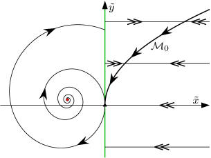
Figure B.3: For HLB 20, a sketch of the local dynamics in the limit $\mu\to 0^{+}$. Note, $\tilde{x}$ is defined by (B.48) for the left half-system and by (B.51) for the right half-system.

With small $\mu>0$ and given $\tilde{r}>0$, the forward orbit of $(0,\tilde{r})$ approaches $\mathcal{M}_{0}$ on the fast time-scale, then evolves near $\mathcal{M}_{0}$ on the slow time-scale until intersecting $\tilde{x}=0$ near the origin. In the limit $\mu\to 0$, the orbit arrives at the origin, thus $\lim_{\mu\to 0}P_{R}(\tilde{r};\mu)=0$, with evolution time $T_{R}$ satisfying $\psi_{T_{R}}(\tilde{r})=0$. From (B.58) we obtain

$$\lim_{\mu\to 0}T_{R}(\tilde{r};\mu)=\kappa\ln\mathopen{}\mathclose{{}\left(1+\frac{a_{2}}{\kappa\beta}\,\tilde{r}}\right).$$ (B.59)

Then

$$\lim_{\mu\to 0}P(\tilde{r};\mu) =P_{L}(0;0)$$

$$=-P_{\rm affine}\mathopen{}\mathclose{{}\left(0;\lambda,\omega,\frac{\beta}{a_{2}}}\right),$$

$$=\frac{\beta}{a_{2}\omega}\,{\rm e}^{\nu\hat{s}(\nu)}\sin\mathopen{}\mathclose{{}\left(\hat{s}(\nu)}\right),$$ (B.60)

where $\nu=\frac{\lambda}{\omega}$, see Lemma 4.6. Also by Lemma 4.6,

$$T_{L}(0;0)=\frac{\hat{s}(\nu)}{\omega}.$$ (B.61)

Thus in this limit $P$ has the unique super-stable fixed point (B.60), and (B.59)–(B.61) explain the limiting period (11.22).

$P_{R}(\tilde{r};\mu)$ is $C^{1}$ because we can perform a multiple time-scale analysis Ku15 on (B.52) to calculate its next order contribution. It follows that $P(\tilde{r};\mu)$ is $C^{1}$ and thus has a unique stable fixed point $\tilde{r}^{*}(\mu)$ (equal to (B.60) in the limit $\mu\to 0$) by the IFT. Hence, in a neighbourhood of the origin, (11.13) has a unique stable limit cycle for sufficiently small $\mu>0$. The order of its minimum and maximum $x$ and $y$-values are explained by the scalings (B.48) and (B.51).

Second consider $\mu<0$. With the scaling

$$\tilde{x} =\frac{x}{\mu^{2}}, \tilde{y} =\frac{y-\zeta(\mu)}{|\mu|},$$ (B.62)

the right half-system becomes

$$\begin{split}|\mu|\dot{\tilde{x}}&=a_{4}\sqrt{\tilde{x}}+a_{2}\tilde{y}+O(\mu),\\ \dot{\tilde{y}}&=\frac{\beta}{a_{2}}+b_{4}\sqrt{\tilde{x}}+b_{2}\tilde{y}+O(\mu).\end{split}$$ (B.63)

The system (B.63) has a unique equilibrium: a stable node $\mathopen{}\mathclose{{}\left(\tilde{x}_{R}^{*},\tilde{y}_{R}^{*}}\right)=\mathopen{}\mathclose{{}\left(\frac{\beta^{2}}{\gamma^{2}},-\frac{a_{4}\beta}{a_{2}\gamma}}\right)+O(\mu)$. It is straight-forward to see that for any $\tilde{r}>0$, the forward orbit of $\mathopen{}\mathclose{{}\left(\tilde{x},\tilde{y}}\right)=\mathopen{}\mathclose{{}\left(0,\tilde{r}}\right)$ rapidly approaches a slow manifold, then slowly approaches $\mathopen{}\mathclose{{}\left(\tilde{x}_{R}^{*},\tilde{y}_{R}^{*}}\right)$. Consequently, locally, (11.13) has no limit cycle when $\mu<0$. ∎

Appendix C Proofs for slipping foci and folds

Proof of Theorem 7.1 (HLB 5).

We first compute regular equilibria and sliding motion to verify part (i) of Theorem 7.1, and then construct and analyse a Poincaré map to verify part (ii).

Write

$$\begin{split}f_{J}(x,y;\mu)&=a_{1J}x+a_{2J}y+a_{3J}\mu+o\mathopen{}\mathclose{{}\left(|x|+|y|+|\mu|}\right),\\ g_{J}(x,y;\mu)&=b_{1J}x+b_{2J}y+b_{3J}\mu+o\mathopen{}\mathclose{{}\left(|x|+|y|+|\mu|}\right),\end{split}$$ (C.1)

for each $J\in\{L,R\}$. Notice $a_{2L}>0$, $a_{2R}>0$, and

$$\gamma=a_{2L}b_{2R}-a_{2R}b_{2L}\,.$$ (C.2)

The boundary equilibria $(0,\xi_{L}(\mu))$ and $(0,\xi_{R}(\mu))$ are clockwise-rotating foci because $a_{2L}>0$ and $a_{2R}>0$. Thus when $\xi_{L}(\mu)<\xi_{R}(\mu)$, as is the case for $\mu<0$ because $\beta>0$ by assumption, $\Gamma$ is an attracting sliding region, see Fig. 7.1. Conversely when $\xi_{L}(\mu)<\xi_{R}(\mu)$, as is the case for $\mu>0$, $\Gamma$ is a repelling sliding region. By evaluating (3.7) we find we can write the sliding vector field as

$$g_{\rm slide}(y;\mu)=\frac{\mathopen{}\mathclose{{}\left(y-\xi_{L}(\mu)}\right)\mathopen{}\mathclose{{}\left(y-\xi_{R}(\mu)}\right)h(y;\mu)}{f_{L}(0,y;\mu)-f_{R}(0,y;\mu)},$$ (C.3)

where $\lim_{(y;\mu)\to(0,0)}h(y;\mu)=\gamma$. With $\mu<0$, in $\Gamma$ we have $f_{L}>0$, $f_{R}<0$, and $\xi_{L}<y<\xi_{R}$. Thus for sufficiently small values of $y$ and $\mu$, if $\gamma<0$ then $g_{\rm slide}>0$ and so $(0,\xi_{R}(\mu))$ is stable, while if $\gamma>0$ then $g_{\rm slide}<0$ and $(0,\xi_{L}(\mu))$ is stable. This verifies part (i).

Now given $r>\xi_{R}(\mu)$, consider the forward orbit of $(x,y)=(0,r)$ that immediately enters $x>0$. Let $P_{R}(r;\mu)$ be the $y$-value of the next intersection of this orbit with $x=0$, and let $T_{R}(r;\mu)$ be the corresponding evolution time. Similarly given $r<\xi_{L}(\mu)$, consider the forward orbit of $(x,y)=(0,r)$ that immediately enters $x<0$. Let $P_{L}(r;\mu)$ be the $y$-value of the next intersection of this orbit with $x=0$, and let $T_{L}(r;\mu)$ be the corresponding evolution time.

Via a change of coordinates that translates $(0,\xi_{R}(\mu))$ to the origin, Lemma 4.4 gives

$$P_{R}(r;\mu)=\xi_{R}(\mu)-{\rm e}^{\frac{\lambda_{R}\pi}{\omega_{R}}}\mathopen{}\mathclose{{}\left(r-\xi_{R}(\mu)}\right)+o\mathopen{}\mathclose{{}\left(|r|+|\mu|}\right),$$ (C.4)

and $T_{R}(r;\mu)\to\frac{\pi}{\omega_{R}}$ as $r\to 0$ (here the ODEs are only $C^{1}$ so we only get the leading order terms of (4.7)–(4.8)). Similarly

$$P_{L}(r;\mu)=\xi_{L}(\mu)-{\rm e}^{\frac{\lambda_{L}\pi}{\omega_{L}}}\mathopen{}\mathclose{{}\left(r-\xi_{L}(\mu)}\right)+o\mathopen{}\mathclose{{}\left(|r|+|\mu|}\right),$$ (C.5)

and $T_{L}(r;\mu)\to\frac{\pi}{\omega_{L}}$ as $r\to 0$.

To accommodate the case $\mu<0$, let $\check{r}(\mu)=P_{R}^{-1}(\xi_{L}(\mu);\mu)=\xi_{R}(\mu)-\beta\,{\rm e}^{\frac{-\lambda_{R}\pi}{\omega_{R}}}\mu+o(\mu)$. Then $P=P_{L}\circ P_{R}$ is well-defined and $C^{1}$ (by Lemma 4.3) for small $r>\check{r}(\mu)$ in the case $\mu<0$, and small $r>\xi_{R}(\mu)$ in the case $\mu>0$. By composing (C.4) and (C.5) we obtain

$$P(r;\mu) =\xi_{R}(\mu)+\mathopen{}\mathclose{{}\left(1+{\rm e}^{\frac{\lambda_{L}\pi}{\omega_{L}}}}\right)\beta\mu$$

$$\quad+{\rm e}^{\alpha\pi}\mathopen{}\mathclose{{}\left(r-\xi_{R}(\mu)}\right)+o\mathopen{}\mathclose{{}\left(|r|+|\mu|}\right).$$ (C.6)

The Poincaré map $P$ is not defined for all $(r;\mu)$ near $(0;0)$, but in view of (C.6) we can extend $P$ so that it is $C^{1}$ throughout a neighbourhood of $(r;\mu)=(0;0)$. This allows to formally apply the IFT to solve $P(r;\mu)=r$, and from this we obtain the unique fixed point

$$r^{*}(\mu)=\xi_{R}(\mu)+\frac{\Big{(}1+{\rm e}^{\frac{\lambda_{L}\pi}{\omega_{L}}}\Big{)}\beta}{1-{\rm e}^{\alpha\pi}}\,\mu+o(\mu),$$ (C.7)

assuming $\alpha\neq 0$.

First suppose $\alpha<0$. If $\mu<0$ then $r^{*}(\mu)<\xi_{R}(\mu)$, which is outside the domain of $P$. Hence $P$ has no fixed points and, locally, (6.1) has no limit cycle. If instead $\mu>0$ then $r^{*}(\mu)>\xi_{R}(\mu)$, so $P$ has a unique fixed point and (6.1) has a unique limit cycle. The limit cycle is stable because $\lim_{\mu\to 0}\frac{\partial P}{\partial r}\mathopen{}\mathclose{{}\left(r^{*}(\mu);\mu}\right)={\rm e}^{\alpha\pi}\in(0,1)$. The limit cycle intersects $x=0$ at $r^{*}(\mu)$ and

$$P_{R}\mathopen{}\mathclose{{}\left(r^{*}(\mu);\mu}\right)=\xi_{L}(\mu)-\frac{\Big{(}1+{\rm e}^{\frac{\lambda_{R}\pi}{\omega_{R}}}\Big{)}\beta}{1-{\rm e}^{\alpha\pi}}\,\mu+o(\mu),$$

and consequently its minimum and maximum $x$ and $y$-values are asymptotically proportional to $|\mu|$. Its period is $T_{L}\mathopen{}\mathclose{{}\left(P_{R}\mathopen{}\mathclose{{}\left(r^{*}(\mu);\mu}\right);\mu}\right)+T_{R}\mathopen{}\mathclose{{}\left(r^{*}(\mu);\mu}\right)$ which limits to $\frac{\pi}{\omega_{L}}+\frac{\pi}{\omega_{R}}$ as $\mu\to 0$.

Finally suppose $\alpha>0$. If $\mu<0$ then (C.7) implies $r^{*}(\mu)>\check{r}(\mu)$. Thus $P$ has a unique fixed point and (6.1) has a unique limit cycle. This limit cycle is unstable because ${\rm e}^{\alpha\pi}>1$ and the above properties hold for its amplitude and period. If instead $\mu>0$ then $r^{*}(\mu)<\xi_{R}(\mu)$ and so (6.1) has no limit cycle. ∎

Proof of Theorem 7.2 (HLB 6).

Here we write

$$\begin{split}f_{L}(x,y;\mu)&=a_{1L}x+a_{2L}y+o\mathopen{}\mathclose{{}\left(|x|+|y|+|\mu|}\right),\\ g_{L}(x,y;\mu)&=b_{1L}x+b_{2L}y+o\mathopen{}\mathclose{{}\left(|x|+|y|+|\mu|}\right),\end{split}$$ (C.8)

where $a_{2L}>0$, and

$$\begin{split}f_{R}(x,y;\mu)&=a_{1R}x+a_{2R}y+a_{3R}\mu\\ &\quad+o\mathopen{}\mathclose{{}\left(|x|+|y|+|\mu|}\right),\\ g_{R}(x,y;\mu)&=b_{0R}+b_{1R}x+b_{2R}y+b_{3R}\mu\\ &\quad+o\mathopen{}\mathclose{{}\left(|x|+|y|+|\mu|}\right),\end{split}$$ (C.9)

where $a_{2R}>0$, $a_{3R}=\beta$, and $b_{0R}<0$.

The $y$-value of the fold is $\zeta_{R}(\mu)=-\frac{\beta}{a_{2R}}\,\mu+o(\mu)$. Since $\beta>0$, for $\mu<0$ we have $\zeta_{R}(\mu)>0$ and consequently $\Gamma$ is an attracting sliding region. Conversely for $\mu>0$ we have $\zeta_{R}(\mu)<0$ and $\Gamma$ is a repelling sliding region. Through (3.7) we obtain

$$g_{\rm slide}(y;\mu)=\frac{yh(y;\mu)}{f_{L}(0,y;\mu)-f_{R}(0,y;\mu)},$$ (C.10)

where $\lim_{(y;\mu)\to(0,0)}h(y;\mu)=a_{2L}b_{0R}$. Thus with $\mu<0$, on $\Gamma$ we have $y>0$ and so $g_{\rm slide}(y;\mu)<0$ (because $a_{2L}b_{0R}<0$). Therefore sliding orbits approach the origin and so the origin is a stable stationary solution. With instead $\mu>0$ the origin is unstable because $f_{R}(0,0;\mu)>0$.

Define the return maps $P_{R}$ and $P_{L}$ and return times $T_{R}$ and $T_{L}$ as in the proof of Theorem 7.1, see Fig. C.1. Via a change of coordinates that translates $(0,\zeta_{R}(\mu))$ to the origin, Lemma 4.5 gives

$$P_{R}(r;\mu)=2\zeta_{R}(\mu)-r+o\mathopen{}\mathclose{{}\left(|r|+|\mu|}\right),$$ (C.11)

and $T_{R}(r;\mu)=O(1)$. Also Lemma 4.4 gives

$$P_{L}(r;\mu)=-{\rm e}^{\frac{\lambda_{L}\pi}{\omega_{L}}}\,r+o\mathopen{}\mathclose{{}\left(|r|+|\mu|}\right),$$ (C.12)

and $T_{L}(r;\mu)\to\frac{\pi}{\omega_{L}}$ as $r\to 0$.

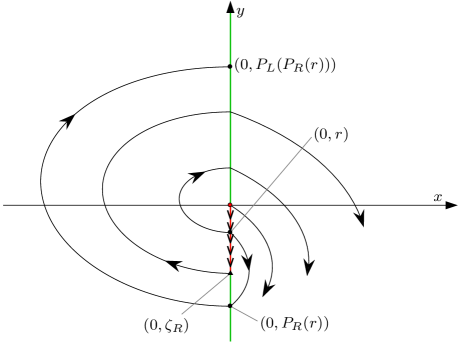
Figure C.1: A phase portrait illustrating the Poincaré map $P=P_{L}\circ P_{R}$ for HLB 6.

Let $\check{r}(\mu)=P_{R}^{-1}(0;\mu)=2\zeta_{R}(\mu)+o(\mu)$. The Poincaré map $P=P_{L}\circ P_{R}$ is well-defined and $C^{1}$ for $r>\check{r}(\mu)$ in the case $\mu<0$, and for $r>\zeta_{R}(\mu)$ in the case $\mu>0$. By composing (C.11) and (C.12) we obtain

$$P(r;\mu)={\rm e}^{\frac{\alpha\pi}{\omega_{L}}}\mathopen{}\mathclose{{}\left(r+\frac{2\beta}{a_{2R}}\,\mu}\right)+o\mathopen{}\mathclose{{}\left(|r|+|\mu|}\right).$$ (C.13)

By using the IFT to solve for fixed points of $P$ (as in the proof of Theorem 7.1) we obtain the locally unique value

$$r^{*}(\mu)=\frac{2\beta}{a_{2R}\mathopen{}\mathclose{{}\left({\rm e}^{\frac{-\alpha\pi}{\omega_{L}}}-1}\right)}\,\mu+o(\mu),$$ (C.14)

assuming $\alpha\neq 0$. The proof is completed by determining the admissibility and stability $r^{*}(\mu)$ as in the proof of Theorem 7.1 (we omit these details for brevity). Note that the maximum $x$-value attained by the orbit segment associated with $P_{R}(r;\mu)$ is asymptotically proportional to $\mathopen{}\mathclose{{}\left(r-\zeta_{R}(\mu)}\right)^{2}$ and for this reason the maximum $x$-value of the limit cycle is asymptotically proportional to $\mu^{2}$. ∎

Proof of Theorem 7.18 (HLB 7).

We write

$$\begin{split}f_{J}(x,y;\mu)&=a_{1J}x+a_{2J}y+a_{3J}\mu\\ &\quad+O\mathopen{}\mathclose{{}\left(\mathopen{}\mathclose{{}\left(|x|+|y|+|\mu|}\right)^{2}}\right),\\ g_{J}(x,y;\mu)&=b_{0J}+b_{1J}x+b_{2J}y+b_{3J}\mu\\ &\quad+O\mathopen{}\mathclose{{}\left(\mathopen{}\mathclose{{}\left(|x|+|y|+|\mu|}\right)^{2}}\right),\end{split}$$ (C.15)

where

$$a_{2L} >0, a_{2R} >0, b_{0L} >0, b_{0R} <0.$$ (C.16)

By the IFT, locally we have $f_{J}(0,\zeta_{J}(\mu);\mu)=0$ for a unique $C^{2}$ function $\zeta_{J}(\mu)=-\frac{a_{3J}}{a_{2J}}\,\mu+O\mathopen{}\mathclose{{}\left(\mu^{2}}\right)$. The folds $(0,\zeta_{L}(\mu))$ and $(0,\zeta_{R}(\mu))$ are the endpoints of $\Gamma$. Notice

$$\zeta_{L}(\mu)-\zeta_{R}(\mu)=\beta\mu+O\mathopen{}\mathclose{{}\left(\mu^{2}}\right).$$ (C.17)

Since $\beta>0$, for $\mu<0$ we have $\zeta_{L}(\mu)<\zeta_{R}(\mu)$ and so $\Gamma$ is an attracting sliding region. With instead $\mu>0$ we have $\zeta_{L}(\mu)>\zeta_{R}(\mu)$ and $\Gamma$ is a repelling sliding region.

From (3.7) we obtain

$$g_{\rm slide}(y;\mu)=\frac{-\mathopen{}\mathclose{{}\left(a_{2R}b_{0L}-a_{2L}b_{0R}}\right)y+\mathopen{}\mathclose{{}\left(a_{3L}b_{0R}-a_{3R}b_{0L}}\right)\mu+O\mathopen{}\mathclose{{}\left(\mathopen{}\mathclose{{}\left(|y|+|\mu|}\right)^{2}}\right)}{f_{L}(0,y;\mu)-f_{R}(0,y;\mu)}.$$ (C.18)

Solving $\dot{y}_{\rm slide}(y;\mu)=0$ reveals (by the IFT) a unique pseudo-equilibrium at $\mathopen{}\mathclose{{}\left(0,y_{\rm eq}(\mu)}\right)$ where

$$y_{\rm eq}(\mu)=\frac{a_{3L}b_{0R}-a_{3R}b_{0L}}{a_{2R}b_{0L}-a_{2L}b_{0R}}\,\mu+O\mathopen{}\mathclose{{}\left(\mu^{2}}\right).$$ (C.19)

We can write (C.19) as the convex combination

$$y_{\rm eq}(\mu)=\mathopen{}\mathclose{{}\left(1-s(\mu)}\right)\zeta_{L}(\mu)+s(\mu)\zeta_{R}(\mu),$$

where

$$s(\mu)=\frac{a_{2R}b_{0L}}{a_{2R}b_{0L}-a_{2L}b_{0R}}.$$

Notice (C.16) implies $s(\mu)\in(0,1)$, thus $\mathopen{}\mathclose{{}\left(0,y_{\rm eq}(\mu)}\right)$ lies within the sliding region $\Gamma$. Therefore $\mathopen{}\mathclose{{}\left(0,y_{\rm eq}(\mu)}\right)$ is admissible and is the unique stationary solution of (6.1). The pseudo-equilibrium $\mathopen{}\mathclose{{}\left(0,y_{\rm eq}(\mu)}\right)$ is unstable when $\mu>0$ because here $\Gamma$ is repelling; it is stable when $\mu<0$ because here $\Gamma$ is attracting and

$$\frac{\partial g_{\rm slide}}{\partial y}\mathopen{}\mathclose{{}\left(y_{\rm eq}(\mu);\mu}\right)=-\frac{a_{2R}b_{0L}-a_{2L}b_{0R}}{f_{L}\mathopen{}\mathclose{{}\left(0,y_{\rm eq}(\mu);\mu}\right)-f_{R}\mathopen{}\mathclose{{}\left(0,y_{\rm eq}(\mu);\mu}\right)}$$

is negative.

Define the return maps $P_{R}$ and $P_{L}$ and return times $T_{R}$ and $T_{L}$ as in the proof of Theorem 7.1. Via a change of coordinates that translates $(0,\zeta_{R}(\mu))$ to the origin, Lemma 4.5 gives

$$P_{R}(r;\mu)=2\zeta_{R}(\mu)-r+\frac{2\sigma_{R}}{3}\mathopen{}\mathclose{{}\left(r-\zeta_{R}(\mu)}\right)^{2}+o\mathopen{}\mathclose{{}\left(\mathopen{}\mathclose{{}\left(|r|+|\mu|}\right)^{2}}\right),$$ (C.20)

where $\sigma_{R}=\sigma_{\rm fold}[f_{R}(x,y;0),g_{R}(x,y;0)]$ (here we are evaluating (4.12) using $f_{R}(x,y;0)$ and $g_{R}(x,y;0)$ in place of the functions $f(x,y)$ and $g(x,y)$ of §4). Also $T_{R}(r;\mu)=\frac{-2}{b_{0R}}\,r+O(2)$. Similarly

$$P_{L}(r;\mu)=2\zeta_{L}(\mu)-r+\frac{2\sigma_{L}}{3}\mathopen{}\mathclose{{}\left(r-\zeta_{L}(\mu)}\right)^{2}+o\mathopen{}\mathclose{{}\left(\mathopen{}\mathclose{{}\left(|r|+|\mu|}\right)^{2}}\right),$$ (C.21)

where $\sigma_{L}=\sigma_{\rm fold}[f_{L}(x,y;0),g_{L}(x,y;0)]$ and $T_{L}(r;\mu)=\frac{-2}{b_{0L}}\,r+O(2)$.

Locally the Poincaré map $P=P_{L}\circ P_{R}$ is well-defined and $C^{2}$ for $r>\check{r}(\mu)=P_{R}^{-1}(\zeta_{L}(\mu);\mu)$ in the case $\mu<0$ and for $r>\zeta_{R}(\mu)$ in the case $\mu>0$. By composing (C.20) and (C.21) we obtain

$$P(r;\mu)=r+2\beta\mu+\frac{2\alpha}{3}\,r^{2}+\kappa_{1}\mu r+\kappa_{2}\mu^{2}+o\mathopen{}\mathclose{{}\left(\mathopen{}\mathclose{{}\left(|r|+|\mu|}\right)^{2}}\right),$$ (C.22)

where we have substituted (C.17) and $\alpha=\sigma_{L}-\sigma_{R}$. Formulas for $\kappa_{1},\kappa_{2}\in\mathbb{R}$ will not be needed. We can extend $P$ so that it is $C^{2}$ throughout a neighbourhood of $(r;\mu)=(0;0)$, then apply the IFT to solve $P(r;\mu)=r$, not for $r$, but for $\mu$ (this is possible because $\frac{\partial P}{\partial\mu}(0;0)=2\beta\neq 0$). This yields a unique $C^{2}$ function $\mu=h(r)=-\frac{\alpha}{3\beta}\,r^{2}+o\mathopen{}\mathclose{{}\left(r^{2}}\right)$.

Now suppose $\alpha<0$. Then $h(r)\geq 0$, so if $\mu<0$ then $P$ has no fixed point and (6.1) has no limit cycle, while if $\mu>0$ then $P$ has a unique fixed point

$$r^{*}(\mu)=\sqrt{\frac{-3\beta\mu}{\alpha}}+o\mathopen{}\mathclose{{}\left(\sqrt{\mu}}\right),$$ (C.23)

and (6.1) has a unique limit cycle. This limit cycle is stable because $\frac{\partial P}{\partial r}\mathopen{}\mathclose{{}\left(r^{*}(\mu);\mu}\right)=1+\frac{2\alpha r^{*}(\mu)}{3}+O(\mu)$ has modulus less than $1$. Its maximum $y$-value is $r^{*}(\mu)$, while its maximum $x$-value is asymptotically proportional to $\mu$ because the maximum $x$-value attained by the orbit segment associated with $P_{R}(r;\mu)$ is asymptotically proportional to $\mathopen{}\mathclose{{}\left(r-\zeta_{R}(\mu)}\right)^{2}$. The minimum $x$ and $y$-values of the limit cycle evidently have the same asymptotic behaviour. The period of the limit cycle is $T_{L}\mathopen{}\mathclose{{}\left(P_{R}\mathopen{}\mathclose{{}\left(r^{*}(\mu);\mu}\right);\mu}\right)+T_{R}\mathopen{}\mathclose{{}\left(r^{*}(\mu);\mu}\right)=\mathopen{}\mathclose{{}\left(\frac{2}{b_{0L}}-\frac{2}{b_{0R}}}\right)r^{*}(\mu)+O(\mu)$ which verifies (7.18). The result in the case $\alpha>0$ follows similarly. ∎

Appendix D Proofs for fixed foci and folds

For the proofs of Theorems 8.6–8.23 we can assume without loss of generality that both half-systems involve clockwise rotation and use the following definition for the components of the Poincaré map $P=P_{L}\circ P_{R}$, see Fig. 4.1. Given $r>0$, let $P_{R}(r;\mu)$ denote the $y$-value at which the forward orbit of $(x,y)=(0,r)$ next intersects $x=0$, and let $T_{R}(r;\mu)$ be the corresponding evolution time. Similarly given $r<0$, let $P_{L}(r;\mu)$ denote the $y$-value at which the forward orbit of $(x,y)=(0,r)$ next intersects $x=0$, and let $T_{L}(r;\mu)$ be the corresponding evolution time.

Proof of Theorem 8.6 (HLB 8).

From Lemma 4.4 we obtain

$$P_{R}(r;\mu) =-{\rm e}^{\frac{\lambda_{R}\pi}{\omega_{R}}}r+{\rm e}^{\frac{\lambda_{R}\pi}{\omega_{R}}}\mathopen{}\mathclose{{}\left({\rm e}^{\frac{\lambda_{R}\pi}{\omega_{R}}}+1}\right)\chi_{R}r^{2}+o\mathopen{}\mathclose{{}\left(r^{2}}\right),$$

$$P_{L}(r;\mu) =-{\rm e}^{\frac{\lambda_{L}\pi}{\omega_{L}}}r+{\rm e}^{\frac{\lambda_{L}\pi}{\omega_{L}}}\mathopen{}\mathclose{{}\left({\rm e}^{\frac{\lambda_{L}\pi}{\omega_{L}}}+1}\right)\chi_{L}r^{2}+o\mathopen{}\mathclose{{}\left(r^{2}}\right),$$

where we have omitted ‘focus’ from the subscripts of $\chi$ for brevity. By composing these and substituting $\Lambda(\mu)=\beta\mu+O\mathopen{}\mathclose{{}\left(\mu^{2}}\right)$ and $\chi_{L}(0)-\chi_{R}(0)=\alpha$, we obtain

$$P(r;\mu)=r+\beta\pi\mu r+\alpha\mathopen{}\mathclose{{}\left({\rm e}^{\frac{\lambda_{R}\pi}{\omega_{R}}}+1}\right)r^{2}+o\mathopen{}\mathclose{{}\left(\mathopen{}\mathclose{{}\left(|r|+|\mu|}\right)^{2}}\right).$$ (D.1)

By construction, $r=0$ is a fixed point of $P$ for all sufficiently small values of $\mu$. This corresponds to the boundary equilibrium at the origin. We have $\frac{\partial P}{\partial r}(0;\mu)=1+\beta\pi\mu+o(\mu)$, thus if $\mu<0$ then $\frac{\partial P}{\partial r}(0;\mu)<1$ in a neighbourhood of $r=0$ and so the origin is stable, while if $\mu>0$ then $\frac{\partial P}{\partial r}(0;\mu)>1$ in a neighbourhood of $r=0$ and the origin is unstable.

Since $P$ is $C^{2}$ and $P(0;\mu)=0$ for all $\mu$, the function $D(r;\mu)=\frac{1}{r}\mathopen{}\mathclose{{}\left(P(r;\mu)-r}\right)$ is $C^{1}$. Moreover we can extend its domain to a neighbourhood of $(r;\mu)=(0;0)$. This allows us to use the IFT to solve $D(r;\mu)=0$ for $r$ (because $\frac{\partial D}{\partial r}(0;0)\neq 0$ assuming $\alpha\neq 0$) to obtain

$$r^{*}(\mu)=\frac{-\beta\pi}{\alpha\Big{(}{\rm e}^{\frac{\lambda_{R}\pi}{\omega_{R}}}+1\Big{)}}\,\mu+o(\mu).$$ (D.2)

This is valid (i.e. $r^{*}(\mu)>0$) when $\alpha\mu<0$ and corresponds to a limit cycle of (6.1). Thus, locally, (6.1) has no limit cycle if $\alpha\mu>0$ and a unique limit cycle if $\alpha\mu<0$. Since $\frac{\partial P}{\partial r}\mathopen{}\mathclose{{}\left(r^{*}(\mu);\mu}\right)=1-\beta\pi\mu+o(\mu)$, the stability of the limit cycle is opposite to that of the origin. The statements regarding the size of the limit cycle follow from (D.2). Finally, Lemma 4.4 also gives $T_{R}(r;\mu)=\frac{\pi}{\omega_{R}(\mu)}+O(r)$ and $T_{L}(r;\mu)=\frac{\pi}{\omega_{L}(\mu)}+O(r)$ which explain (8.6). ∎

Proof of Theorem 8.17 (HLB 9).

From Lemmas 4.4 and 4.5 we obtain

$$P_{R}(r;\mu) =-r+\frac{2\sigma_{{\rm fold},R}}{3}\,r^{2}+o\mathopen{}\mathclose{{}\left(r^{2}}\right),$$ (D.3)

$$P_{L}(r;\mu) =-{\rm e}^{\frac{\lambda_{L}\pi}{\omega_{L}}}r+{\rm e}^{\frac{\lambda_{L}\pi}{\omega_{L}}}\mathopen{}\mathclose{{}\left({\rm e}^{\frac{\lambda_{L}\pi}{\omega_{L}}}+1}\right)\chi_{{\rm focus},L}\,r^{2}+o\mathopen{}\mathclose{{}\left(r^{2}}\right),$$ (D.4)

Since $\lambda_{L}(\mu)=\beta\mu+o(\mu)$, we can replace each instance of ${\rm e}^{\frac{\lambda_{L}\pi}{\omega_{L}}}$ in (D.4) with $1+\frac{\beta\pi}{\omega_{L}(0)}\,\mu+o(\mu)$. Then by composing (D.3) and (D.4) we obtain

$$P(r;\mu)=r+\frac{\beta\pi}{\omega_{L}(0)}\,\mu r+2\alpha r^{2}+o\mathopen{}\mathclose{{}\left(\mathopen{}\mathclose{{}\left(|r|+|\mu|}\right)^{2}}\right),$$ (D.5)

where we have also used $\chi_{{\rm focus},L}(0)-\frac{\sigma_{{\rm fold},R}(0)}{3}=\alpha$.

As in the proof of Theorem 8.6, $P$ has at most two fixed points: $r=0$, corresponding to the origin, and

$$r^{*}(\mu)=\frac{-\beta\pi}{2\alpha\omega_{L}(0)}\,\mu+o(\mu),$$ (D.6)

which is valid when $\alpha\mu<0$ and corresponds to a limit cycle. The stability of the origin and limit cycle can be determined from the sign of $\frac{\partial P}{\partial r}-1$, as in the previous proof. The extremal $x$ and $y$ values of the limit cycle are asymptotically proportional to $|\mu|$ by (D.6), except the maximum $x$-value is asymptotically proportional to $\mu^{2}$ due to the fold of the right half-system. Finally, Lemmas 4.4 and 4.5 also give $T_{R}(r;\mu)=\frac{-2}{g_{R}(0,0;\mu)}\,r+O\mathopen{}\mathclose{{}\left(r^{2}}\right)$ and $T_{L}(r;\mu)=\frac{\pi}{\omega_{L}(\mu)}+O(r)$, and the sum of these produces (8.17). ∎

Proof of Theorem 8.23 (HLB 10).

Lemma 4.5 gives

$$P_{R}(r;\mu) =-r+\frac{2\sigma_{R}}{3}\,r^{2}-\frac{4\sigma_{R}^{2}}{9}r^{3}+\frac{2\chi_{R}}{15}r^{4}+o\mathopen{}\mathclose{{}\left(r^{4}}\right),$$

$$P_{L}(r;\mu) =-r+\frac{2\sigma_{L}}{3}\,r^{2}-\frac{4\sigma_{L}^{2}}{9}r^{3}+\frac{2\chi_{L}}{15}r^{4}+o\mathopen{}\mathclose{{}\left(r^{4}}\right),$$

where we have omitted ‘fold’ from the subscripts of $\sigma$ and $\chi$ for brevity. By composing these we obtain

$$P(r;\mu)=r+\frac{2}{3}(\sigma_{L}-\sigma_{R})r^{2}+\frac{4}{9}(\sigma_{L}-\sigma_{R})^{2}r^{3}+\mathopen{}\mathclose{{}\left(\frac{2}{15}(\chi_{L}-\chi_{R})-\frac{8}{9}\sigma_{L}\sigma_{R}(\sigma_{L}-\sigma_{R})}\right)r^{4}+o\mathopen{}\mathclose{{}\left(r^{4}}\right).$$ (D.7)

By then substituting $\sigma_{L}(\mu)-\sigma_{R}(\mu)=\beta\mu+O\mathopen{}\mathclose{{}\left(\mu^{2}}\right)$ and $\chi_{L}(0)-\chi_{R}(0)=\alpha$ we arrive at

$$P(r;\mu)=r+\mathopen{}\mathclose{{}\left(\frac{2\beta\mu}{3}+O\mathopen{}\mathclose{{}\left(\mu^{2}}\right)}\right)r^{2}+\frac{2\alpha}{15}r^{4}+o\mathopen{}\mathclose{{}\left(\mathopen{}\mathclose{{}\left(|r|+|\mu|}\right)^{4}}\right).$$ (D.8)

This map has the fixed point $r=0$ (corresponding to the two-fold at the origin) which from $\frac{\partial P}{\partial r}$ we see is stable for $\mu<0$ and unstable for $\mu>0$ (because $\beta>0$). To formally obtain a second fixed point we first observe that $P$ is $C^{4}$ for small $r>0$ because $F_{L}$ and $F_{R}$ are $C^{4}$ (see Lemma 4.3). It is a simple exercise to show that $D(r;\mu)=\frac{1}{r^{2}}\mathopen{}\mathclose{{}\left(P(r;\mu)-r}\right)$ is $C^{2}$. Moreover, $D$ can be extended in a $C^{2}$ fashion to a neighbourhood of $(r;\mu)=(0,0)$. We can then use the IFT to solve $D(r;\mu)=0$ for $\mu$ (possible because $\frac{\partial D}{\partial\mu}=\frac{2\beta}{3}\neq 0$), and by inverting the result we obtain the fixed point

$$r^{*}(\mu)=\sqrt{\frac{-5\beta\mu}{\alpha}}+o\mathopen{}\mathclose{{}\left(\sqrt{|\mu|}}\right).$$ (D.9)

Under the restriction $r>0$, this point exists and is unique when $\alpha\mu<0$ and corresponds to a limit cycle of (6.1). The period of the limit cycle is $T_{L}\mathopen{}\mathclose{{}\left(P_{R}\mathopen{}\mathclose{{}\left(r^{*}(\mu);\mu}\right);\mu}\right)+T_{R}\mathopen{}\mathclose{{}\left(r^{*}(\mu);\mu}\right)$, where $T_{R}(r;\mu)=\frac{-2}{g_{R}(0,0;\mu)}\,r+O\mathopen{}\mathclose{{}\left(r^{2}}\right)$ and $T_{L}(r;\mu)=\frac{-2}{g_{L}(0,0;\mu)}\,r+O\mathopen{}\mathclose{{}\left(r^{2}}\right)$ by Lemma 4.5, and these combine to produce (8.23). ∎

Appendix E Proofs for impacting systems

We may write the vector field of (9.1) subject to (9.3) and (9.5) as

$$\begin{split}f(x,y;\mu)&=a_{1}x+a_{2}y+o\mathopen{}\mathclose{{}\left(|x|+|y|+|\mu|}\right),\\ g(x,y;\mu)&=b_{1}x+b_{2}y+b_{3}\mu+o\mathopen{}\mathclose{{}\left(|x|+|y|+|\mu|}\right).\end{split}$$ (E.1)

Notice $a_{2}>0$ and $\beta=-a_{2}b_{3}$. Thus $\beta>0$ implies $b_{3}<0$. Let

$$A={\rm D}F(0,0;0)=\begin{bmatrix}a_{1}&a_{2}\\ b_{1}&b_{2}\end{bmatrix}.$$

Assuming $\det(A)\neq 0$, locally there exists a unique regular equilibrium $\mathopen{}\mathclose{{}\left(x^{*}(\mu),y^{*}(\mu)}\right)$ with

$$x^{*}(\mu)=\frac{-\beta}{\det(A)}\,\mu+o(\mu).$$ (E.2)

Proof of Lemma 9.1.

By (E.2) we have $\mathopen{}\mathclose{{}\left(x^{*}(\mu),y^{*}(\mu)}\right)\in\Omega_{L}$ when $\mu>0$. Since $\det(A)>0$, if $\lambda<0$ then $\mathopen{}\mathclose{{}\left(x^{*}(\mu),y^{*}(\mu)}\right)$ is a stable node or focus, while if $\lambda>0$ then $\mathopen{}\mathclose{{}\left(x^{*}(\mu),y^{*}(\mu)}\right)$ is a unstable node or focus.

Now suppose $\mu<0$ and the consider the forward orbit of $(x,y)=(0,r)$ where $r>0$. This point is mapped to $(0,-\gamma r+o(r))$, then, since the origin is an invisible fold, evolves in $\Omega_{L}$ and next intersects $x=0$ at $y=\gamma r+o(r)$ by Lemma 4.5. Thus the sign of $\ln(\gamma)$ determines the stability of the pseudo-equilibrium. ∎

Proof of Theorems 9.2–9.4 (HLBs 11–13).

Here we derive and analyse two Poincaré maps, one for $\mu<0$ and one for $\mu>0$, assuming $\beta>0$ and $\lambda\ln(\gamma)<0$. From the fixed points of these maps, subject to different assumptions on the values of $\alpha$ and $\omega$, we are able to verify all statements in Theorems 9.2–9.4. In view of the substitution $(x,y,t)\mapsto(x,-y,-t)$, we assume $\lambda>0$ which implies $\gamma<1$.

First suppose $\mu>0$. By Lemma 9.1 the system has an unstable regular equilibrium in $\Omega_{L}$. Let

$$\tilde{x} =\frac{x}{\mu}, \tilde{y} =\frac{y}{\mu},$$ (E.3)

with which the ODEs become

$$\begin{split}\dot{\tilde{x}}&=a_{1}\tilde{x}+a_{2}\tilde{y}+O(\mu),\\ \dot{\tilde{y}}&=b_{3}+b_{1}\tilde{x}+b_{2}\tilde{y}+O(\mu).\end{split}$$ (E.4)

The impact law becomes $\tilde{y}\mapsto\tilde{\phi}(\tilde{y})=\frac{1}{\mu}\phi\mathopen{}\mathclose{{}\left(\mu\tilde{y}}\right)$ and observe

$$\tilde{\phi}(\tilde{y})=-\gamma\tilde{y}+O(\mu).$$ (E.5)

For any $\tilde{r}<0$, let $P_{L}(\tilde{r};\mu)$ be the $\tilde{y}$-component of the next intersection of the forward orbit of $(0,\tilde{r})$ with $\tilde{x}=0$ (leave $P_{L}(\tilde{r};\mu)$ undefined if this orbit does not return to $\tilde{x}=0$). Also let $T_{L}(\tilde{r};\mu)$ be the corresponding evolution time. Then, given $\tilde{r}>0$, our Poincaré map is

$$P(\tilde{r};\mu)=P_{L}\big{(}\tilde{\phi}(\tilde{r});\mu\big{)},$$ (E.6)

see Fig. E.1, corresponding to an evolution time of

$$T(\tilde{r};\mu)=T_{L}\big{(}\tilde{\phi}(\tilde{r});\mu\big{)},$$ (E.7)

because the impact law is assumed to be instantaneous.

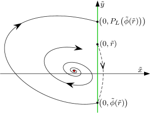
Figure E.1: An illustration of the Poincaré map (E.6) for HLBs 11–12 with $\mu>0$.

As in the proof of Theorem 6.2, we now study the scaled system in the limit $\mu\to 0$. With $\mu=0$ the ODEs (E.4) are affine and the impact law (E.5) is linear. In the case that the regular equilibrium is a node (HLB 13), as in the proof of Theorem 5.2 we can use the slow invariant subspace of the node to demonstrate that the system has no limit cycle (we omit these arguments for brevity). Now suppose the regular equilibrium is a focus (HLBs 11–12). By Lemma 4.6,

$$\begin{split}P_{L}(\tilde{r};0)&=-P_{\rm affine}\mathopen{}\mathclose{{}\left(-\tilde{r};\lambda,\omega,-b_{3}}\right),\\ T_{L}(\tilde{r};0)&=T_{\rm affine}\mathopen{}\mathclose{{}\left(-\tilde{r};\lambda,\omega,-b_{3}}\right),\end{split}$$ (E.8)

which are of Type III because $\lambda>0$ and $b_{3}<0$.

By (4.25)–(4.26), any fixed point of $P(\tilde{r};0)$, call it $\tilde{r}^{*}$, satisfies

$$\begin{split}\gamma\tilde{r}^{*}&=\frac{-\kappa{\rm e}^{-\lambda T_{0}}\varrho\mathopen{}\mathclose{{}\left(\omega T_{0};\frac{\lambda}{\omega}}\right)}{\sin(\omega T_{0})},\\ -\tilde{r}^{*}&=\frac{\kappa{\rm e}^{\lambda T_{0}}\varrho\mathopen{}\mathclose{{}\left(\omega T_{0};-\frac{\lambda}{\omega}}\right)}{\sin(\omega T_{0})}\end{split}$$ (E.9)

where $T_{0}=T_{L}(\tilde{r}^{*};0)$ and $\kappa=\frac{-b_{3}\omega}{\lambda^{2}+\omega^{2}}$. Note that these combine to produce the desired formula (9.10). Using (4.27) we obtain

$$\frac{\partial P}{\partial\tilde{r}}(\tilde{r};0)=\frac{\gamma^{2}\tilde{r}}{P_{L}(-\gamma\tilde{r};0)}\,{\rm e}^{2\lambda T_{L}(-\gamma\tilde{r};0)},$$ (E.10)

and with $\tilde{r}=\tilde{r}^{*}$ this simplifies to

$$\frac{\partial P}{\partial\tilde{r}}(\tilde{r}^{*};0)=\gamma^{2}{\rm e}^{2\lambda T_{L}(-\gamma\tilde{r}^{*};0)}.$$ (E.11)

In the next few steps we use the fact that $T_{L}(-\gamma\tilde{r};0)$ is a decreasing function of $\tilde{r}$ (by Lemma 4.6).

As in the proof of Theorem 6.2, suppose for the moment that $P(\tilde{r};0)$ has a fixed point and let $\tilde{r}^{*}$ be the smallest such point. Since $P(0;0)>0$, we must have $P(\tilde{r};0)>\tilde{r}$ for all $0\leq\tilde{r}<\tilde{r}^{*}$, and so $\frac{\partial P}{\partial\tilde{r}}(\tilde{r}^{*};0)\leq 1$. Actually $\frac{\partial P}{\partial\tilde{r}}(\tilde{r}^{*};0)<1$ because $\frac{\partial P}{\partial\tilde{r}}\mathopen{}\mathclose{{}\left(\tilde{r}^{*};0}\right)=1$ implies $\frac{\partial^{2}P}{\partial\tilde{r}^{2}}\mathopen{}\mathclose{{}\left(\tilde{r}^{*};0}\right)=2\lambda\frac{d}{d\tilde{r}}T_{L}(-\gamma\tilde{r}^{*};0)<0$ which is not possible. Since $\tilde{r}^{*}$ is the smallest fixed point, by (E.11) we must have $\frac{\partial P}{\partial\tilde{r}}<1$ at every fixed point. Hence $P(\tilde{r};0)$ has no other fixed points and so $P(\tilde{r};0)<\tilde{r}$ for all $\tilde{r}>\tilde{r}^{*}$.

This situation requires $\alpha\leq 0$ because as $\tilde{r}\to\infty$ we have $P(\tilde{r};0)\sim\gamma\,{\rm e}^{\frac{\lambda\pi}{\omega}}\tilde{r}={\rm e}^{\alpha}\tilde{r}$ (see Lemma 4.6). Thus in the case $\alpha>0$ (HLB 12), $P(\tilde{r};0)$ has no fixed points (and thus (9.1) has no limit cycle), while if $\alpha<0$ (HLB 11) then $P(\tilde{r};0)$ has a fixed point by the intermediate value theorem and, as we have just shown, this point is unique and asymptotically stable. Since $P$ is $C^{1}$ the fixed point persists for small $\mu>0$ and corresponds to a stable limit cycle of (9.1) of size asymptotically proportional to $\mu$ (see the final part of the proof of Theorem 6.2 for details).

Second suppose $\mu<0$. Let

$$\tilde{x} =-\frac{x}{\mu}, \tilde{y} =-\frac{y}{\mu},$$ (E.12)

with which the ODEs become

$$\begin{split}\dot{\tilde{x}}&=a_{1}\tilde{x}+a_{2}\tilde{y}+O(\mu),\\ \dot{\tilde{y}}&=-b_{3}+b_{1}\tilde{x}+b_{2}\tilde{y}+O(\mu)\end{split}$$ (E.13)

We define $P_{L}$ and $T_{L}$ as above but now have

$$\begin{split}P_{L}(\tilde{r};0)&=-P_{\rm affine}\mathopen{}\mathclose{{}\left(-\tilde{r};\lambda,\omega,b_{3}}\right),\\ T_{L}(\tilde{r};0)&=T_{\rm affine}\mathopen{}\mathclose{{}\left(-\tilde{r};\lambda,\omega,b_{3}}\right),\end{split}$$ (E.14)

which are of Type I because $b_{3}<0$ and $\omega={\rm i}\eta$ in the case of HLB 13. Again any fixed point $\tilde{r}^{*}$ of $P(\tilde{r};0)$, defined by (E.6), satisfies (E.9) where $T_{0}=T_{L}(\tilde{r}^{*};0)$, but now $\kappa=\frac{b_{3}\omega}{\lambda^{2}+\omega^{2}}$. Thus again we have (9.10).

Since $P_{\rm affine}$ is of Type I we have $P(\tilde{r};0)\to 0$ as $\tilde{r}\to 0$. Moreover $\frac{\partial P}{\partial\tilde{r}}(\tilde{r};0)\to\gamma$ as $\tilde{r}\to 0$ (as in the proof of Lemma 9.1). Thus if $\tilde{r}^{*}$ is the smallest positive fixed point of $P(\tilde{r};0)$ then $\frac{\partial P}{\partial\tilde{r}}(\tilde{r}^{*};0)\geq 1$. By repeating the above arguments we can show that $\frac{\partial P}{\partial\tilde{r}}(\tilde{r}^{*};0)<1$ and, if it exists, $\tilde{r}^{*}$ is the only positive fixed point of $P(\tilde{r};0)$.

If the regular equilibrium is a focus (HLBs 11–12) then again $P(\tilde{r};0)\sim{\rm e}^{\alpha}\tilde{r}$ as $\tilde{r}\to\infty$. Thus if $\alpha<0$ (HLB 11), $P(\tilde{r};0)$ has no fixed points (and thus (9.1) has no limit cycle), while if $\alpha>0$ (HLB 12) then $P(\tilde{r};0)$ has a fixed point by the intermediate value theorem and this point is unique and unstable. Since $P$ is $C^{1}$ it persists for small $\mu<0$ and corresponds to an unstable limit cycle of (9.1).

If the regular equilibrium is a node (HLB 13) then $P(\tilde{r};0)\to\infty$ as $\tilde{r}\to\frac{-b_{3}}{\lambda+\eta}$, thus $P(\tilde{r};0)$ has a fixed point by the intermediate value theorem. As above this point is unique, unstable, persists for small $\mu<0$, and corresponds to an unstable limit cycle of (9.1). ∎

Appendix F Proof for impulsive systems (HLB 14)

For sufficiently small $y>0$, the forward orbit of $(r,\theta)=\mathopen{}\mathclose{{}\left(y,\frac{\pi}{2}}\right)$ undergoes an impulse then evolves via (9.23) until $\theta=-\frac{3\pi}{2}\mapsto\frac{\pi}{2}$ at some $r=P(y;\mu)$ (at which point another impulse is applied). Let $T(y;\mu)$ denote the corresponding evolution time. In order to ’blow up’ the dynamics about the origin we write

$$\tilde{r}=\frac{r}{y},$$

with which

$$\begin{split}\dot{\tilde{r}}&=\lambda\tilde{r}+y\tilde{r}^{2}\mathcal{F}(\theta)+o(y),\\ \dot{\theta}&=-\omega+y\tilde{r}\mathcal{G}(\theta)+o(y).\end{split}$$ (F.1)

Let $\varphi_{t}(\tilde{r},\theta)$ and $\psi_{t}(\tilde{r},\theta)$, respectively, denote the $r$ and $\theta$-components of the flow of (F.1). Then $P(y;\mu)$ and $T(y;\mu)$ satisfy

$$\begin{split}\varphi_{T(y;\mu)}\mathopen{}\mathclose{{}\left(\tfrac{1}{y}R(y;\mu),\Theta(y;\mu)}\right)&=\frac{1}{y}\,P(y;\mu),\\ \psi_{T(y;\mu)}\mathopen{}\mathclose{{}\left(\tfrac{1}{y}R(y;\mu),\Theta(y;\mu)}\right)&=-\frac{3\pi}{2},\end{split}$$ (F.2)

and are $C^{2}$ because the flow intersects the positive $y$-axis transversally.

We write the flow as a series expansion in $y$:

$$\begin{split}\varphi_{t}\mathopen{}\mathclose{{}\left(\tfrac{1}{y}R(y;\mu),\Theta(y;\mu)}\right)&=\Phi^{(0)}_{t}(y;\mu)+y\Phi^{(1)}_{t}(y;\mu)+o(y),\\ \psi_{t}\mathopen{}\mathclose{{}\left(\tfrac{1}{y}R(y;\mu),\Theta(y;\mu)}\right)&=\Psi^{(0)}_{t}(y;\mu)+y\Psi^{(1)}_{t}(y;\mu)+o(y).\end{split}$$ (F.3)

We also write

$$\begin{split}R(y;\mu)&=\gamma y+\zeta y^{2}+o\mathopen{}\mathclose{{}\left(y^{2}}\right),\\ \Theta(y;\mu)&=\phi+\xi y+o(y),\end{split}$$ (F.4)

for some constants $\zeta,\xi\in\mathbb{R}$ and we have neglected the $\mu$-dependency for brevity. By substituting (F.3) into the first equation of (F.1) we obtain

$$\dot{\Phi}^{(0)}_{t}+y\dot{\Phi}^{(1)}_{t}=\lambda\Phi^{(0)}_{t}+y\Big{(}\lambda\Phi^{(1)}_{t}+\Phi^{(0)^{\scriptstyle 2}}_{t}\mathcal{F}\mathopen{}\mathclose{{}\left(\Psi^{(0)}_{t}}\right)\Big{)}+o(y),$$ (F.5)

with initial condition

$$\Phi^{(0)}_{0}+y\Phi^{(1)}_{0}=\gamma+\zeta y+o(y).$$

To first order, $\dot{\Phi}^{(0)}_{t}=\lambda\Phi^{(0)}_{t}$ and $\Phi^{(0)}_{0}=\gamma$, thus

$$\Phi^{(0)}_{t}={\rm e}^{\lambda t}\gamma.$$ (F.6)

Similarly the second equation in (F.1) gives

$$\dot{\Psi}^{(0)}_{t}+y\dot{\Psi}^{(1)}_{t}=-\omega+y\Phi^{(0)}_{t}\mathcal{G}\mathopen{}\mathclose{{}\left(\Psi^{(0)}_{t}}\right)+o(y),$$ (F.7)

with initial condition

$$\Psi^{(0)}_{0}+y\Psi^{(1)}_{0}=\phi+\xi y+o(y).$$

To first order, $\dot{\Psi}^{(0)}_{t}=-\omega$ and $\Psi^{(0)}_{0}=\phi$, thus

$$\Psi^{(0)}_{t}=\phi-\omega t.$$ (F.8)

Next we write $T$ and $P$ as series expansions in $y$:

$$\begin{split}T&=T^{(0)}+yT^{(1)}+o(y),\\ P&=yP^{(0)}+y^{2}P^{(1)}+o\mathopen{}\mathclose{{}\left(y^{2}}\right).\end{split}$$ (F.9)

By substituting (F.8) and (F.9) into the second equation of (F.2) we obtain

$$\phi-\omega T^{(0)}-y\omega T^{(1)}+y\Psi^{(1)}_{T^{(0)}}=-\frac{3\pi}{2}+o(y),$$ (F.10)

and from the constant terms in (F.10) we obtain

$$T^{(0)}=\frac{1}{\omega}\mathopen{}\mathclose{{}\left(\phi+\frac{3\pi}{2}}\right).$$ (F.11)

By similarly substituting (F.6) and (F.9) into the first equation of (F.2) we obtain

$${\rm e}^{\lambda T^{(0)}}\,\gamma+y\lambda T^{(1)}{\rm e}^{\lambda T^{(0)}}\,\gamma+y\Phi^{(1)}_{T^{(0)}}=P^{(0)}+yP^{(1)}+o(y),$$ (F.12)

and from the constant terms in (F.12) we obtain

$$P^{(0)}=\gamma{\rm e}^{\lambda T^{(0)}}={\rm e}^{\Lambda}.$$

Thus

$$P^{(0)}(\mu)=1+\beta\mu+o(\mu).$$ (F.13)

In order to complete the proof it suffices to evaluate $P^{(1)}$ at $\mu=0$. Thus we now set $\mu=0$ with which $\Lambda=0$. Then the $y$-terms in (F.10) and (F.12) imply

$$T^{(1)} =\frac{1}{\omega}\,\Psi^{(1)}_{T^{(0)}},$$

$$P^{(1)} =\Phi^{(1)}_{T^{(0)}}+\frac{\lambda}{\omega}\,\Psi^{(1)}_{T^{(0)}}.$$ (F.14)

Next we show that $P^{(1)}(0)=\alpha$ (9.25).

The $y$-terms in (F.5) give $\dot{\Phi}^{(1)}_{t}=\lambda\Phi^{(1)}_{t}+{\rm e}^{2\lambda t}\,\gamma^{2}\mathcal{F}(\phi-\omega t)$ and $\Phi^{(1)}_{0}=\zeta$, thus

$$\Phi^{(1)}_{t}={\rm e}^{\lambda t}\mathopen{}\mathclose{{}\left(\zeta+\gamma^{2}\int_{0}^{t}{\rm e}^{\lambda s}\,\mathcal{F}(\phi-\omega s)\,ds}\right).$$

By substituting (F.11) (and using $\Lambda=0$ and $\theta=\phi-\omega s$) we obtain

$$\Phi^{(1)}_{T^{(0)}}=\frac{\zeta}{\gamma}+\frac{1}{\omega}\,{\rm e}^{\frac{-3\pi\lambda}{2\omega}}\int_{\frac{-3\pi}{2}}^{\phi}{\rm e}^{\frac{-\lambda\theta}{\omega}}\,\mathcal{F}(\theta)\,d\theta.$$ (F.15)

Similarly the $y$-terms in (F.7) give $\dot{\Psi}^{(1)}_{t}={\rm e}^{\lambda t}\,\gamma\mathcal{G}(\phi-\omega t)$ and $\Psi^{(1)}_{0}=\xi$, thus

$$\Psi^{(1)}_{t}=\xi+\int_{0}^{t}{\rm e}^{\lambda s}\,\gamma\mathcal{G}(\phi-\omega s)\,ds,$$

and by substituting (F.11) we arrive at

$$\Psi^{(1)}_{T^{(0)}}=\xi+\frac{1}{\omega}\,{\rm e}^{\frac{-3\pi\lambda}{2\omega}}\int_{\frac{-3\pi}{2}}^{\phi}{\rm e}^{\frac{-\lambda\theta}{\omega}}\,\mathcal{G}(\theta)\,d\theta.$$ (F.16)

In summary we have shown

$$P(y;\mu)=y+\beta\mu y+\alpha y^{2}+o\mathopen{}\mathclose{{}\left(\mathopen{}\mathclose{{}\left(|y|+|\mu|}\right)^{2}}\right),$$ (F.17)

for sufficiently small values of $y\geq 0$ and $\mu\in\mathbb{R}$. Locally $P$ has at most two fixed points: $y=0$, corresponding to the boundary equilibrium at the origin, and

$$y^{*}(\mu)=-\frac{\beta}{\alpha}\,\mu+o(\mu),$$ (F.18)

which is valid when $y^{*}(\mu)>0$ and corresponds to a limit cycle (formally (F.18) can be obtained via the IFT by solving for zeros of $\frac{1}{y}\mathopen{}\mathclose{{}\left(P(y;\mu)-y}\right)$ as in the proof of Theorem 8.6). Since $\beta>0$, the system has a unique limit cycle if $\alpha\mu<0$ and no limit cycle if $\alpha\mu>0$. The limit cycle intersects the positive $y$-axis at $y^{*}(\mu)$, thus has amplitude asymptotically proportional to $|\mu|$. Its period is given by (F.11), to leading order.

Stability is determined from

$$\frac{\partial P}{\partial y}(y;\mu)=1+\beta\mu+2\alpha y+o\mathopen{}\mathclose{{}\left(|y|+|\mu|}\right).$$

Observe $\frac{\partial P}{\partial y}(0;\mu)=1+\beta\mu+o(\mu)$, thus the origin is stable if $\mu<0$ and is unstable if $\mu>0$. Also $\frac{\partial P}{\partial y}\mathopen{}\mathclose{{}\left(y^{*}(\mu);\mu}\right)=1-\beta\mu+o(\mu)$, thus the stability of the limit cycle is opposite to that of the origin. $\Box$

Appendix G Proofs for hysteresis

Proof of Theorem 10.8 (HLB 15).

For each $J\in\{L,R\}$, write

$$\begin{split}f_{J}(x,y)&=a_{0J}+a_{1J}x+a_{2J}y+O\mathopen{}\mathclose{{}\left(\mathopen{}\mathclose{{}\left(|x|+|y|}\right)^{2}}\right),\\ g_{J}(x,y)&=b_{0J}+b_{1J}x+b_{2J}y+O\mathopen{}\mathclose{{}\left(\mathopen{}\mathclose{{}\left(|x|+|y|}\right)^{2}}\right),\end{split}$$ (G.1)

where $a_{0R}<0<a_{0L}$. The assumption (10.6) implies

$$\frac{b_{0L}}{a_{0L}}=\frac{b_{0R}}{a_{0R}}.$$ (G.2)

Also

$$\alpha=a_{0L}b_{2R}+a_{2L}b_{0R}-a_{0R}b_{2L}-a_{2R}b_{0L}\,.$$ (G.3)

Let $\varphi^{R}_{t}(x,y)$ and $\psi^{R}_{t}(x,y)$, respectively, denote the $x$ and $y$-components of the flow of $F_{R}$. By asymptotic matching we obtain

$$\begin{split}\varphi^{R}_{t}(\mu,y)&=\mu+a_{0R}t+a_{1R}\mu t+a_{2R}yt\\ &\quad+\frac{a_{0R}a_{1R}+a_{2R}b_{0R}}{2}\,t^{2}+o\mathopen{}\mathclose{{}\left(\mathopen{}\mathclose{{}\left(|y|+|\mu|+|t|}\right)^{2}}\right),\\ \psi^{R}_{t}(\mu,y)&=y+b_{0R}t+b_{1R}\mu t+b_{2R}yt\\ &\quad+\frac{a_{0R}b_{1R}+b_{0R}b_{2R}}{2}\,t^{2}+o\mathopen{}\mathclose{{}\left(\mathopen{}\mathclose{{}\left(|y|+|\mu|+|t|}\right)^{2}}\right).\end{split}$$ (G.4)

Define $P_{R}(r;\mu)$ and $T_{R}(r;\mu)$ by

$$\varphi^{R}_{T_{R}(r;\mu)}\mathopen{}\mathclose{{}\left(\mu,r}\right) =-\mu$$ (G.5)

$$\psi^{R}_{T_{R}(r;\mu)}\mathopen{}\mathclose{{}\left(\mu,r}\right) =P_{R}(r;\mu),$$ (G.6)

see Fig. G.1. Using (G.4) we obtain

$$T_{R}(r;\mu) =\frac{-2}{a_{0R}}\,\mu+\frac{2a_{2R}}{a_{0R}^{2}}\,\mu r-\frac{2a_{2R}b_{0R}}{a_{0R}^{3}}\,\mu^{2}$$

$$\quad+o\mathopen{}\mathclose{{}\left(\mathopen{}\mathclose{{}\left(|r|+|\mu|}\right)^{2}}\right),$$ (G.7)

$$P_{R}(r;\mu) =r-\frac{2b_{0R}}{a_{0R}}\,\mu+c_{1R}\mu r+c_{2R}\mu^{2}$$

$$\quad+o\mathopen{}\mathclose{{}\left(\mathopen{}\mathclose{{}\left(|r|+|\mu|}\right)^{2}}\right),$$ (G.8)

where we define

$$c_{1J}=\frac{2\mathopen{}\mathclose{{}\left(a_{2J}b_{0J}-a_{0J}b_{2J}}\right)}{a_{0J}^{2}},$$ (G.9)

for each $J\in\{L,R\}$ (a formula for $c_{2R}$ will not be needed).

Define $P_{L}(r;\mu)$ and $T_{L}(r;\mu)$ analogously, Fig. G.1. Via the replacement $(R,\mu)\mapsto(L,-\mu)$ in (G.7)–(G.8) we obtain

$$T_{L}(r;\mu) =\frac{2}{a_{0L}}\,\mu-\frac{2a_{2L}}{a_{0L}^{2}}\,\mu r-\frac{2a_{2L}b_{0L}}{a_{0L}^{3}}\,\mu^{2}$$

$$\quad+o\mathopen{}\mathclose{{}\left(\mathopen{}\mathclose{{}\left(|r|+|\mu|}\right)^{2}}\right),$$ (G.10)

$$P_{L}(r;\mu) =r+\frac{2b_{0L}}{a_{0L}}\,\mu-c_{1L}\mu r+c_{2L}\mu^{2}$$

$$\quad+o\mathopen{}\mathclose{{}\left(\mathopen{}\mathclose{{}\left(|r|+|\mu|}\right)^{2}}\right),$$ (G.11)

where $c_{2L}\in\mathbb{R}$.

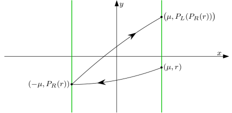
Figure G.1: An illustration of the Poincaré map $P=P_{L}\circ P_{R}$ for HLB 15.

Let $P=P_{L}\circ P_{R}$ be our Poincaré map. This corresponds to an evolution time of

$$T(r;\mu)=T_{R}(r;\mu)+T_{L}\mathopen{}\mathclose{{}\left(P_{R}(r;\mu);\mu}\right).$$ (G.12)

By composing (G.8) and (G.11) we obtain

$$P(r;\mu) =r+2\mathopen{}\mathclose{{}\left(\frac{b_{0L}}{a_{0L}}-\frac{b_{0R}}{a_{0R}}}\right)\mu-\mathopen{}\mathclose{{}\left(c_{1L}-c_{1R}}\right)\mu r$$

$$\quad+\mathopen{}\mathclose{{}\left(c_{2L}+c_{2R}}\right)\mu^{2}+o\mathopen{}\mathclose{{}\left(\mathopen{}\mathclose{{}\left(|r|+|\mu|}\right)^{2}}\right),$$

and via careful use of (G.2), (G.3), and (G.9) we find this reduces to

$$P(r;\mu)=r+\frac{2\alpha}{a_{0L}a_{0R}}\,\mu r+\mathopen{}\mathclose{{}\left(c_{2L}+c_{2R}}\right)\mu^{2}+o\mathopen{}\mathclose{{}\left(\mathopen{}\mathclose{{}\left(|r|+|\mu|}\right)^{2}}\right).$$ (G.13)

Since $P$ is $C^{2}$ and $P(r;0)=r$ for all $r$, the function $D(r;\mu)=\frac{1}{\mu}\mathopen{}\mathclose{{}\left(P(r;\mu)-r}\right)$ is $C^{1}$. Its domain can be extended so that it is $C^{1}$ throughout a neighbourhood of $(r;\mu)=(0;0)$. If $\alpha\neq 0$ the IFT then implies the existence of a unique $C^{1}$ function $r^{*}(\mu)$ such that $D\mathopen{}\mathclose{{}\left(r^{*}(\mu);\mu}\right)=0$ for all values of $\mu$ in a neighbourhood of $0$, and

$$r^{*}(\mu)=\frac{a_{0L}a_{0R}\mathopen{}\mathclose{{}\left(c_{2L}+c_{2R}}\right)}{2\alpha}\,\mu+o\mathopen{}\mathclose{{}\left(\mu}\right).$$ (G.14)

Notice $r^{*}(\mu)$ is a fixed point of $P(r;\mu)$ and corresponds to a limit cycle of (10.2). Since $\frac{\partial P}{\partial r}(r;\mu)=1-\frac{2\alpha\mu}{a_{0L}a_{0R}}+o\mathopen{}\mathclose{{}\left(|r|+|\mu|}\right)$, the limit cycle is stable if $\alpha<0$ and unstable if $\alpha>0$. From (G.7), (G.10), and (G.12) we see that its period is given by (10.8). ∎

Proof of Theorem 10.17 (HLB 17).

For each $J\in\{L,R\}$, write

$$\begin{split}f_{J}(x,y)&=a_{1J}x+a_{2J}y+a_{3J}x^{2}+a_{4J}xy+a_{5J}y^{2}\\ &\quad+O\mathopen{}\mathclose{{}\left(\mathopen{}\mathclose{{}\left(|x|+|y|}\right)^{3}}\right),\\ g_{J}(x,y)&=b_{0J}+b_{1J}x+b_{2J}y+b_{3J}x^{2}+b_{4J}xy+b_{5J}y^{2}\\ &\quad+O\mathopen{}\mathclose{{}\left(\mathopen{}\mathclose{{}\left(|x|+|y|}\right)^{3}}\right).\end{split}$$ (G.15)

Without loss of generality we assume clockwise rotation, thus

$$a_{2L} >0, a_{2R} >0,$$ (G.16)

$$b_{0L} >0, b_{0R} <0.$$

Also

$$\sigma_{{\rm fold},J}=\frac{a_{1J}}{b_{0J}}+\frac{b_{2J}}{b_{0J}}-\frac{a_{5J}}{a_{2J}}.$$ (G.17)

As in the previous proof, let $\varphi^{R}_{t}(x,y)$ and $\psi^{R}_{t}(x,y)$, respectively, denote the $x$ and $y$-components of the flow of $F_{R}$ and define $P_{R}(r;\mu)$ and $T_{R}(r;\mu)$ by (G.5)–(G.6). By asymptotic matching we obtain

$$\varphi^{R}_{t}\mathopen{}\mathclose{{}\left(\mu,r}\right) =\mu+a_{1R}\mu t+a_{2R}rt+\frac{a_{2R}b_{0R}}{2}\,t^{2}+a_{3R}\mu^{2}t+a_{4R}\mu rt+a_{5R}r^{2}t+\mathopen{}\mathclose{{}\left(\frac{a_{1R}^{2}}{2}+\frac{a_{2R}b_{1R}}{2}+\frac{a_{4R}b_{0R}}{2}}\right)\mu t^{2}$$

$$\quad+\mathopen{}\mathclose{{}\left(\frac{a_{1R}a_{2R}}{2}+\frac{a_{2R}b_{2R}}{2}+a_{5R}b_{0R}}\right)rt^{2}+\mathopen{}\mathclose{{}\left(\frac{a_{1R}a_{2R}b_{0R}}{6}+\frac{a_{2R}b_{0R}b_{2R}}{6}+\frac{a_{5R}b_{0R}^{2}}{3}}\right)t^{3}+o\mathopen{}\mathclose{{}\left(\mathopen{}\mathclose{{}\left(|\mu|+|r|+|t|}\right)^{3}}\right),$$ (G.18)

$$\psi^{R}_{t}(\mu,r) =r+b_{0R}t+b_{1R}\mu t+b_{2R}rt+\frac{b_{0R}b_{2R}}{2}\,t^{2}+O\mathopen{}\mathclose{{}\left(\mathopen{}\mathclose{{}\left(|\mu|+|r|+|t|}\right)^{3}}\right),$$ (G.19)

where we have not stated the cubic terms of $\psi^{R}_{t}$ as we will not need them. Away from $(r;\mu)=(0;0)$ the forward orbit of $(x,y)=(\mu,r)$ intersects $x=-\mu$ transversally and so $P_{R}$ and $T_{R}$ are $C^{3}$ functions of $r$ and $\mu$ by Lemma 4.3.

We wish to solve (G.5) for $t=T_{R}(r;\mu)$. Since $\varphi^{R}_{t}\mathopen{}\mathclose{{}\left(\mu,r}\right)$ has no $t$-term we cannot use the IFT to solve (G.5) for $t$. But (G.5) does have a $\mu$-term so we can solve for $\mu$. First observe that if $\mu=0$ then (G.5) has two solutions: $t=0$ and $t=\frac{-2}{b_{0R}}\,r+O\mathopen{}\mathclose{{}\left(r^{2}}\right)$. We are only interested in extending the second solution to $\mu>0$ because the first solution corresponds to backwards evolution for $\mu>0$. Hence we substitute the form

$$t=\frac{-2}{b_{0R}}\,r+S,$$

into (G.18). By the IFT there exists a unique $C^{3}$ function $h$ such that $\varphi^{R}_{t}(h(r,S),r)=-\mu$ throughout a neighbourhood of $(r,S)=(0,0)$. Moreover, we can write this function as

$$h(r,S)=\frac{a_{2R}}{2}\,rS-\frac{a_{2R}\sigma_{{\rm fold},R}}{3b_{0R}}r^{3}+o\mathopen{}\mathclose{{}\left(\mathopen{}\mathclose{{}\left(|r|+\sqrt{|S|}}\right)^{3}}\right),$$ (G.20)

where we have substituted (G.17) and only explicitly stated the terms that will be needed below (e.g. the $S^{2}$-term in (G.20) is not needed). In summary, $T_{R}(r;\mu)=\frac{-2}{b_{0R}}r+S$, where $S$ is given implicitly by $\mu=h(r,S)$.

Recall, $P_{R}$ is defined by (G.6). Here we show that

$$P_{R}(r;\mu)=-\sqrt{r^{2}+c_{1R}\mu+c_{2R}\,r^{3}+o\mathopen{}\mathclose{{}\left(\big{(}\big{|}\mu^{\frac{1}{3}}\big{|}+|r|\big{)}^{3}}\right)},$$ (G.21)

and obtain formulas for $c_{1R},c_{2R}\in\mathbb{R}$. By replacing $\mu$ in (G.21) with (G.20), we obtain

$$P_{R}(r;\mu)^{2} =r^{2}+\frac{a_{2R}c_{1R}}{2}\,rS+\mathopen{}\mathclose{{}\left(c_{2R}-\frac{a_{2R}c_{1R}\sigma_{{\rm fold},R}}{3b_{0R}}}\right)r^{3}$$

$$\quad+o\mathopen{}\mathclose{{}\left(\mathopen{}\mathclose{{}\left(|r|+\sqrt{|S|}}\right)^{3}}\right).$$ (G.22)

By putting $t=\frac{-2}{b_{0R}}\,r+S$ into (G.19) we obtain

$$\psi^{R}_{T_{R}}(\mu,r)=-r+b_{0R}S+O\mathopen{}\mathclose{{}\left(\mathopen{}\mathclose{{}\left(|r|+\sqrt{|S|}}\right)^{3}}\right),$$

and so

$$\psi^{R}_{T_{R}}(\mu,r)^{2}=r^{2}-2b_{0R}rS+o\mathopen{}\mathclose{{}\left(\mathopen{}\mathclose{{}\left(|r|+\sqrt{|S|}}\right)^{3}}\right).$$ (G.23)

Asymptotic matching of (G.22) and (G.23) yields

$$c_{1R} =\frac{-4b_{0R}}{a_{2R}}, c_{2R} =\frac{-4\sigma_{{\rm fold},R}}{3},$$ (G.24)

and justifies the form (G.21). This completes our derivation of $P_{R}$.

We define $P_{L}$ and $T_{L}$ analogously and (repeating the above calculations) obtain

$$P_{L}(r;\mu)=\sqrt{r^{2}+\frac{4b_{0L}}{a_{2L}}\,\mu-\frac{4\sigma_{{\rm fold},L}}{3}\,r^{3}+o\mathopen{}\mathclose{{}\left(\big{(}\big{|}\mu^{\frac{1}{3}}\big{|}+|r|\big{)}^{3}}\right)},$$ (G.25)

and $T_{L}(r;\mu)=\frac{2}{b_{0L}}r+O\mathopen{}\mathclose{{}\left(\big{(}\big{|}\mu^{\frac{1}{3}}\big{|}+|r|\big{)}^{2}}\right)$. As usual let $P=P_{L}\circ P_{R}$. Then by composing (G.21) and (G.25) we arrive at

$$P(r;\mu)=\sqrt{r^{2}+4\kappa\mu+\frac{4\alpha}{3}\,r^{3}+o\mathopen{}\mathclose{{}\left(\big{(}\big{|}\mu^{\frac{1}{3}}\big{|}+|r|\big{)}^{3}}\right)},$$ (G.26)

where $\kappa$ and $\alpha$ are given by (10.14) and (10.16).

To compute fixed points of $P$ in a formal manner we search for zeros of the modified displacement function

$$D(r;\mu) =P(r;\mu)^{2}-r^{2}$$ (G.27)

$$=4\kappa\mu+\frac{4\alpha}{3}\,r^{3}+o\mathopen{}\mathclose{{}\left(\big{(}\big{|}\mu^{\frac{1}{3}}\big{|}+|r|\big{)}^{3}}\right).$$ (G.28)

Since $\kappa\neq 0$, the equation $D(r;\mu)=0$ has a locally unique $C^{3}$ solution $\mu$ (by the IFT) which we can invert to produce

$$r^{*}(\mu)=\mathopen{}\mathclose{{}\left(\frac{-3\kappa}{\alpha}}\right)^{\frac{1}{3}}\mu^{\frac{1}{3}}+o\mathopen{}\mathclose{{}\left(\mu^{\frac{1}{3}}}\right),$$ (G.29)

assuming $\alpha\neq 0$. If $r^{*}(\mu)<0$, this is not a valid fixed point of $P$ because $P\geq 0$ in view of (G.26). We are only interested in $\mu>0$, thus if $\alpha>0$, $P$ has no fixed points (because $\kappa>0$), while if $\alpha<0$, $P$ has the unique fixed point $r^{*}(\mu)$. This value corresponds to a stable limit cycle because $D$ is a decreasing function of $r$.

The maximum $y$-value of the limit cycle is $r^{*}(\mu)$; similarly its minimum $y$-value is asymptotically proportional to $\mu^{\frac{1}{3}}$. Since both half-systems have an invisible fold (quadratic tangency) at the origin, the minimum and maximum $x$-values of the limit cycle are asymptotically proportional to the square of the minimum and maximum $y$-values (this can be established formally via (G.18)).

The evolution time associated with $P(r;\mu)$ is

$$T(r;\mu)=T_{R}(r;\mu)+T_{L}\mathopen{}\mathclose{{}\left(P_{R}(r;\mu);\mu}\right),$$ (G.30)

hence the period of the limit cycle is $T=\mathopen{}\mathclose{{}\left(\frac{2}{b_{0L}}-\frac{2}{b_{0R}}}\right)r^{*}(\mu)+o\mathopen{}\mathclose{{}\left(\mu^{\frac{1}{3}}}\right)$. ∎

Appendix H Proofs for time delay

Let us first describe the behaviour of a typical orbit of (10.3) crossing $x=0$. Let $p(t)\in\mathbb{R}^{2}$ denote the location of the orbit at time $t$. Suppose $p(0)=(0,r)$ for some $r\in\mathbb{R}$. Further suppose there exists $J\in\{L,R\}$ such that $p(t)\in\Omega_{J}$ for all $t\in(-\mu,0)$ and $p(t)\notin\Omega_{J}$ for arbitrarily small $t>0$. Then the orbit next experiences a switch at $p(\mu)=\big{(}G_{J}(r;\mu),H_{J}(r;\mu)\big{)}$ where we define $G_{J}(r;\mu)=\varphi^{J}_{\mu}(0,r)$ and $H_{J}(r;\mu)=\psi^{J}_{\mu}(0,r)$ and where $\varphi^{J}_{t}(x,y)$ and $\psi^{J}_{t}(x,y)$ denote the $x$ and $y$-components of the flow of $F_{J}$. By varying $r$ (and keeping $\mu>0$ fixed) the points $\big{(}G_{L}(r;\mu),H_{L}(r;\mu)\big{)}$ and $\big{(}G_{R}(r;\mu),H_{R}(r;\mu)\big{)}$ trace out curves where orbits of (10.3) experience a switch; these are shown green in Fig. H.1.

Next we define a Poincaré map $P$ (this will be well-defined locally subject to the assumptions of Theorems 10.9 and 10.19). Let $P_{R}(r;\mu)$ denote the $y$-value of the first intersection of the forward orbit of $\mathopen{}\mathclose{{}\left(G_{L}(r;\mu),H_{L}(r;\mu)}\right)$ with $x=0$ following the right half-system and let $T_{R}(r;\mu)$ denote the corresponding evolution time, Fig. H.1. These are defined implicitly by

$$0 =\varphi^{R}_{T_{R}(r;\mu)}\mathopen{}\mathclose{{}\left(G_{L}(r;\mu),H_{L}(r;\mu)}\right),$$ (H.1)

$$P_{R}(r;\mu) =\psi^{R}_{T_{R}(r;\mu)}\mathopen{}\mathclose{{}\left(G_{L}(r;\mu),H_{L}(r;\mu)}\right).$$ (H.2)

Similarly let $P_{L}(r;\mu)$ denote the $y$-value of the first intersection of the forward orbit of $\mathopen{}\mathclose{{}\left(G_{R}(r;\mu),H_{R}(r;\mu)}\right)$ with $x=0$ following the left half-system, and let $T_{L}(r;\mu)$ denote the corresponding evolution time. Then let $P=P_{L}\circ P_{R}$. This corresponds to an evolution time of

$$T(y;\mu)=2\mu+T_{R}(y;\mu)+T_{L}\mathopen{}\mathclose{{}\left(P_{R}(y;\mu);\mu}\right).$$ (H.3)

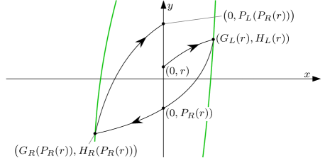
Figure H.1: An illustration of the Poincaré map $P=P_{L}\circ P_{R}$ for HLB 16.

Proof of Theorem 10.9 (HLB 16).

As in the proof of Theorem 10.8, we write

$$\begin{split}f_{J}(x,y)&=a_{0J}+a_{1J}x+a_{2J}y+O\mathopen{}\mathclose{{}\left(\mathopen{}\mathclose{{}\left(|x|+|y|}\right)^{2}}\right),\\ g_{J}(x,y)&=b_{0J}+b_{1J}x+b_{2J}y+O\mathopen{}\mathclose{{}\left(\mathopen{}\mathclose{{}\left(|x|+|y|}\right)^{2}}\right),\end{split}$$ (H.4)

where $a_{0R}<0<a_{0L}$ and we have (G.2) and (G.3).

By using asymptotic matching to calculate the first few terms of the flow of the left half-system, we obtain

$$\begin{split}G_{L}(r;\mu)&=a_{0L}\mu+a_{2L}r\mu+\frac{a_{0L}a_{1L}+a_{2L}b_{0L}}{2}\,\mu^{2}\\ &\quad+o\mathopen{}\mathclose{{}\left(\mathopen{}\mathclose{{}\left(|r|+|\mu|}\right)^{2}}\right),\\ H_{L}(r;\mu)&=r+b_{0L}\mu+b_{2L}r\mu+\frac{a_{0L}b_{1L}+b_{0L}b_{2L}}{2}\,\mu^{2}\\ &\quad+o\mathopen{}\mathclose{{}\left(\mathopen{}\mathclose{{}\left(|r|+|\mu|}\right)^{2}}\right).\end{split}$$ (H.5)

Similarly via asymptotic matching of the right half-system, from (H.1)–(H.2) we obtain

$$T_{R}(r;\mu) =\frac{-1}{a_{0R}}\,G_{L}+\frac{a_{0R}a_{1R}-a_{2R}b_{0R}}{2a_{0R}^{3}}\,G_{L}^{2}$$

$$\quad+\frac{a_{2R}}{a_{0R}^{2}}\,G_{L}H_{L}+o\mathopen{}\mathclose{{}\left(\mathopen{}\mathclose{{}\left(|r|+|\mu|}\right)^{2}}\right),$$ (H.6)

$$P_{R}(r;\mu) =H_{L}-\frac{b_{0R}}{a_{0R}}\,G_{L}$$

$$\quad-\frac{a_{2R}b_{0R}^{2}-a_{0R}b_{0R}\mathopen{}\mathclose{{}\left(a_{1R}+b_{2R}}\right)+a_{0R}^{2}b_{1R}}{2a_{0R}^{3}}\,G_{L}^{2}$$

$$\quad+\frac{a_{2R}b_{0R}-a_{0R}b_{2R}}{a_{0R}^{2}}\,G_{L}H_{L}+o\mathopen{}\mathclose{{}\left(\mathopen{}\mathclose{{}\left(|r|+|\mu|}\right)^{2}}\right).$$ (H.7)

By combining (H.5)–(H.7) we obtain

$$T_{R}(r;\mu) =-\frac{a_{0L}}{a_{0R}}\,\mu+O\mathopen{}\mathclose{{}\left(\mathopen{}\mathclose{{}\left(|r|+|\mu|}\right)^{2}}\right),$$ (H.8)

$$P_{R}(r;\mu) =r+c_{1R}r\mu+c_{2R}\mu^{2}+o\mathopen{}\mathclose{{}\left(\mathopen{}\mathclose{{}\left(|r|+|\mu|}\right)^{2}}\right),$$ (H.9)

where

$$c_{1R}=\frac{a_{0R}b_{2L}-a_{2L}b_{0R}}{a_{0R}}+\frac{a_{0L}\mathopen{}\mathclose{{}\left(a_{2R}b_{0R}-a_{0R}b_{2R}}\right)}{a_{0R}^{2}},$$ (H.10)

while a formula for $c_{2R}\in\mathbb{R}$ will not be needed.

By symmetry we can simply swap the $L$’s and $R$’s in (H.8)–(H.9) to obtain

$$T_{L}(r;\mu) =\frac{-a_{0R}}{a_{0L}}\,\mu+O\mathopen{}\mathclose{{}\left(\mathopen{}\mathclose{{}\left(|r|+|\mu|}\right)^{2}}\right),$$ (H.11)

$$P_{L}(r;\mu) =r+c_{1L}r\mu+c_{2L}\mu^{2}+o\mathopen{}\mathclose{{}\left(\mathopen{}\mathclose{{}\left(|r|+|\mu|}\right)^{2}}\right),$$ (H.12)

where

$$c_{1L}=\frac{a_{0L}b_{2R}-a_{2R}b_{0L}}{a_{0L}}+\frac{a_{0R}\mathopen{}\mathclose{{}\left(a_{2L}b_{0L}-a_{0L}b_{2L}}\right)}{a_{0L}^{2}},$$ (H.13)

and $c_{2L}\in\mathbb{R}$. By then combining the above formulas we arrive at

$$T(r;\mu) =\mathopen{}\mathclose{{}\left(2-\frac{a_{0L}}{a_{0R}}-\frac{a_{0R}}{a_{0L}}}\right)\mu+O\mathopen{}\mathclose{{}\left(\mathopen{}\mathclose{{}\left(|r|+|\mu|}\right)^{2}}\right).$$ (H.14)

$$P(r;\mu) =r+\kappa\alpha r\mu+\mathopen{}\mathclose{{}\left(c_{2L}+c_{2R}}\right)\mu^{2}+o\mathopen{}\mathclose{{}\left(\mathopen{}\mathclose{{}\left(|r|+|\mu|}\right)^{2}}\right),$$ (H.15)

where $\kappa=\frac{a_{0R}-a_{0L}}{a_{0L}a_{0R}}>0$ and $\alpha$ is given by (G.3).

By repeating steps in the proof of Theorem 10.8, we obtain a unique fixed point

$$r^{*}(\mu)=-\frac{c_{2L}+c_{2R}}{\kappa\alpha}\,\mu+o\mathopen{}\mathclose{{}\left(\mu}\right),$$ (H.16)

assuming $\alpha\neq 0$. This fixed point corresponds to a limit cycle of (10.3) with minimum and maximum $x$-values asymptotically proportional to $\mu$. Since $\frac{\partial P}{\partial y}(y;\mu)=1+\kappa\alpha\mu+o(1)$, the limit cycle is stable if $\alpha<0$ and unstable if $\alpha>0$. Its period is given by (H.14) evaluated at $r=r^{*}(\mu)$. ∎

Proof of Theorem 10.19 (HLB 18).

As in the proof of Theorem 10.17, we write the components of $F_{J}$ as (G.15) and assume clockwise rotation (without loss of generality) so that we have (G.16); also (G.17). Here we obtain

$$\begin{split}G_{L}(r;\mu)&=a_{2L}\mu r+\frac{a_{2L}b_{0L}}{2}\,\mu^{2}+O\mathopen{}\mathclose{{}\left(\mathopen{}\mathclose{{}\left(|r|+|\mu|}\right)^{3}}\right),\\ H_{L}(r;\mu)&=r+b_{0L}\mu+b_{2L}\mu r+\frac{b_{0L}b_{2L}}{2}\,\mu^{2}+O\mathopen{}\mathclose{{}\left(\mathopen{}\mathclose{{}\left(|r|+|\mu|}\right)^{3}}\right),\end{split}$$ (H.17)

and

$$\varphi^{R}_{t}\mathopen{}\mathclose{{}\left(G_{L}(r;\mu),H_{L}(r;\mu)}\right) =a_{2L}\mu r+a_{2R}b_{0L}\mu t+a_{2R}rt+\frac{a_{2R}b_{0R}}{2}\,t^{2}+\frac{a_{2L}b_{0L}}{2}\,\mu^{2}+a_{5R}r^{2}t$$

$$\quad+\mathopen{}\mathclose{{}\left(\frac{a_{1R}a_{2R}}{2}+\frac{a_{2R}b_{2R}}{2}+a_{5R}b_{0R}}\right)rt^{2}+\mathopen{}\mathclose{{}\left(\frac{a_{1R}a_{2R}b_{0R}}{6}+\frac{a_{2R}b_{0R}b_{2R}}{6}+\frac{a_{5R}b_{0R}^{2}}{3}}\right)t^{3}$$

$$\quad+U+o\mathopen{}\mathclose{{}\left(\mathopen{}\mathclose{{}\left(|r|+|\mu|+|t|}\right)^{3}}\right),$$ (H.18)

$$\psi^{R}_{t}\mathopen{}\mathclose{{}\left(G_{L}(r;\mu),H_{L}(r;\mu)}\right) =r+b_{0L}\mu+b_{0R}t+b_{2R}rt+\frac{b_{0R}b_{2R}}{2}\,t^{2}+b_{2L}\mu r+b_{0L}b_{2R}\mu t+\frac{b_{0L}b_{2L}}{2}\,\mu^{2}$$

$$\quad+O\mathopen{}\mathclose{{}\left(\mathopen{}\mathclose{{}\left(|r|+|\mu|+|t|}\right)^{3}}\right),$$ (H.19)

where $U$ represents all third order terms involving $\mu$ (these will not be needed below).

By using (H.18) to solve (H.1) we obtain

$$T_{R}(r;\mu) =\frac{-2}{b_{0R}}\,r+\mathopen{}\mathclose{{}\left(\frac{a_{2L}}{a_{2R}}-\frac{2b_{0L}}{b_{0R}}}\right)\mu+\frac{2\sigma_{{\rm fold},R}}{3b_{0R}}\,r^{2}+c_{1R}\mu r+c_{2R}\mu^{2}+o\mathopen{}\mathclose{{}\left(\mathopen{}\mathclose{{}\left(|r|+|\mu|}\right)^{2}}\right),$$ (H.20)

for some $c_{1R},c_{2R}\in\mathbb{R}$. By substituting (H.20) into (H.19) we obtain

$$P_{R}(r;\mu) =-r-a_{2L}\kappa\mu+\frac{2\sigma_{{\rm fold},R}}{3}\,r^{2}+d_{1R}\mu r+d_{2R}\mu^{2}+o\mathopen{}\mathclose{{}\left(\mathopen{}\mathclose{{}\left(|r|+|\mu|}\right)^{2}}\right),$$ (H.21)

for some $d_{1R},d_{2R}\in\mathbb{R}$. Swapping $L$’s and $R$’s gives

$$P_{L}(r;\mu) =-r+a_{2R}\kappa\mu+\frac{2\sigma_{{\rm fold},L}}{3}\,r^{2}+d_{1L}\mu r+d_{2L}\mu^{2}+o\mathopen{}\mathclose{{}\left(\mathopen{}\mathclose{{}\left(|r|+|\mu|}\right)^{2}}\right),$$ (H.22)

where $d_{1L},d_{2L}\in\mathbb{R}$. By composing (H.21) and (H.22) we obtain

$$P(r;\mu) =r+\mathopen{}\mathclose{{}\left(a_{2L}+a_{2R}}\right)\kappa\mu+\frac{2\alpha}{3}\,r^{2}+\ell_{1}\mu r+\ell_{2}\mu^{2}+o\mathopen{}\mathclose{{}\left(\mathopen{}\mathclose{{}\left(|r|+|\mu|}\right)^{2}}\right),$$ (H.23)

for some $\ell_{1},\ell_{2}\in\mathbb{R}$.

As in the proof of Theorem 7.18 we can use the IFT to solve $P(r;\mu)=r$ for $\mu$ and invert to obtain the unique fixed point

$$r^{*}(\mu)=\sqrt{\frac{-3\mathopen{}\mathclose{{}\left(a_{2L}+a_{2R}}\right)\kappa}{2\alpha}}\sqrt{\mu}+o\mathopen{}\mathclose{{}\left(\sqrt{\mu}}\right),$$ (H.24)

assuming $\alpha<0$. This corresponds to the desired limit cycle and is stable because $\frac{\partial P}{\partial r}<1$ at $r=r^{*}(\mu)$.

The maximum $y$-value of the limit cycle is $H_{L}\mathopen{}\mathclose{{}\left(y^{*}(\mu);\mu}\right)=y^{*}(\mu)+o\mathopen{}\mathclose{{}\left(\sqrt{\mu}}\right)$, and the minimum $y$-value is similarly asymptotically proportional to $\sqrt{\mu}$. From (H.18) we find that maximum $x$-value is $-\frac{a_{2R}}{2b_{0R}}\,r^{*}(\mu)^{2}+O(\mu)$, and the minimum $x$-value is similarly asymptotically proportional to $\mu$. Finally, by (H.3), (H.20) (and the analogous formula for $T_{L}$), and (H.24), we see that the period of the limit cycle is given by (10.19). ∎

Appendix I Proof for intersecting switching manifolds (HLB 19)

Given a point $(0,r)$ on the positive $y$-axis, let $P_{1}(r;\mu)$ denote the $x$-value of the first intersection of the forward orbit of $(0,r)$ with the $x$-axis and let $T_{1}(r;\mu)$ denote the corresponding evolution time. Define $P_{2}(r;\mu)$, $P_{3}(r;\mu)$, and $P_{4}(r;\mu)$ similarly, see Fig. I.1, and let $T_{2}(r;\mu)$, $T_{3}(r;\mu)$, and $T_{4}(r;\mu)$ denote the corresponding evolution times. By (11.2) these quantities are well-defined for small values of $r>0$ and $\mu\in\mathbb{R}$. Let

$$P=P_{4}\circ P_{3}\circ P_{2}\circ P_{1}\,,$$ (I.1)

denote the Poincaré map on the positive $y$-axis. The corresponding evolution time is

$$T=T_{1}+T_{2}\circ P_{1}+T_{3}\circ P_{2}\circ P_{1}+T_{4}\circ P_{3}\circ P_{2}\circ P_{1}\,.$$ (I.2)

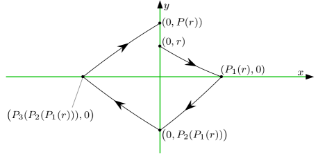
Figure I.1: An illustration of the Poincaré map (I.1) for HLB 19.

For clarity now we suppress the $\mu$-dependency for a moment. We write

$$\begin{split}f_{1}(x,y)&=a_{0}+a_{1}x+a_{2}y+O\mathopen{}\mathclose{{}\left(\mathopen{}\mathclose{{}\left(|x|+|y|}\right)^{2}}\right),\\ g_{1}(x,y)&=b_{0}+b_{1}x+b_{2}y+O\mathopen{}\mathclose{{}\left(\mathopen{}\mathclose{{}\left(|x|+|y|}\right)^{2}}\right),\end{split}$$ (I.3)

where $a_{0}>0$ and $b_{0}<0$. Also

$$m_{1} =\frac{b_{0}}{a_{0}},$$ (I.4)

$$\xi_{1} =\frac{1}{a_{0}}\mathopen{}\mathclose{{}\left(\frac{a_{2}b_{0}}{a_{0}}-(a_{1}+b_{2})+\frac{a_{0}b_{1}}{b_{0}}}\right).$$ (I.5)

Let $\varphi_{t}(x,y)$ and $\psi_{t}(x,y)$ denote the $x$ and $y$-components of the flow of $F_{1}$. By asymptotic matching we obtain

$$\begin{split}\varphi_{t}(0,r)&=a_{0}t+a_{2}rt+\frac{a_{0}a_{1}+a_{2}b_{0}}{2}\,t^{2}+o\mathopen{}\mathclose{{}\left(\mathopen{}\mathclose{{}\left(|r|+|t|}\right)^{2}}\right),\\ \psi_{t}(0,r)&=r+b_{0}t+b_{2}rt+\frac{a_{0}b_{1}+b_{0}b_{2}}{2}\,t^{2}+o\mathopen{}\mathclose{{}\left(\mathopen{}\mathclose{{}\left(|r|+|t|}\right)^{2}}\right).\end{split}$$ (I.6)

Solving $\psi_{t}(0,r)=0$ for $t=T_{1}$ gives

$$T_{1}(r)=\frac{-1}{b_{0}}\,r+\mathopen{}\mathclose{{}\left(\frac{b_{2}}{2b_{0}^{2}}-\frac{a_{0}b_{1}}{2b_{0}^{3}}}\right)r^{2}+o\mathopen{}\mathclose{{}\left(r^{2}}\right).$$ (I.7)

By then using this to evaluate $\varphi_{t}(0,r)$ we obtain

$$P_{1}(r)=\frac{-1}{m_{1}}\,r-\frac{\xi_{1}}{2m_{1}^{2}}\,r^{2}+o\mathopen{}\mathclose{{}\left(r^{2}}\right).$$ (I.8)

Similarly

$$\begin{split}P_{2}(r)&=m_{2}r+\frac{m_{2}\xi_{2}}{2}\,r^{2}+o\mathopen{}\mathclose{{}\left(r^{2}}\right),\\ P_{3}(r)&=\frac{-1}{m_{3}}\,r+\frac{\xi_{3}}{2m_{3}^{2}}\,r^{2}+o\mathopen{}\mathclose{{}\left(r^{2}}\right),\\ P_{4}(r)&=m_{4}r-\frac{m_{4}\xi_{4}}{2}\,r^{2}+o\mathopen{}\mathclose{{}\left(r^{2}}\right),\end{split}$$ (I.9)

and, to leading order,

$$\begin{split}T_{2}(r)&=\frac{-1}{f_{2}(0,0)}\,r+O\mathopen{}\mathclose{{}\left(r^{2}}\right),\\ T_{3}(r)&=\frac{1}{g_{3}(0,0)}\,r+O\mathopen{}\mathclose{{}\left(r^{2}}\right),\\ T_{4}(r)&=\frac{1}{f_{4}(0,0)}\,r+O\mathopen{}\mathclose{{}\left(r^{2}}\right).\end{split}$$ (I.10)

By composing according to (I.1) we obtain

$$P(r)=\Lambda r+\mathopen{}\mathclose{{}\left(\frac{(\xi_{1}-\xi_{2})\Lambda}{2m_{1}}+\frac{(\xi_{3}-\xi_{4})\Lambda^{2}}{2m_{4}}}\right)r^{2}+o\mathopen{}\mathclose{{}\left(r^{2}}\right),$$ (I.11)

where $\Lambda$ is given by (11.3). By evaluating (I.2) we obtain

$$T(r)=\mathopen{}\mathclose{{}\left(\frac{-1}{g_{1}(0,0)}+\frac{1}{m_{1}f_{2}(0,0)}-\frac{\Lambda}{m_{4}f_{3}(0,0)}+\frac{\Lambda}{g_{4}(0,0)}}\right)r+O\mathopen{}\mathclose{{}\left(r^{2}}\right).$$ (I.12)

Now we examine the $\mu$-dependency of $P$. By substituting $\Lambda(\mu)=1+\beta\mu+O\mathopen{}\mathclose{{}\left(\mu^{2}}\right)$ into (I.11) we obtain

$$P(r;\mu)=r+\beta r\mu+\frac{\alpha}{2}\,r^{2}+o\mathopen{}\mathclose{{}\left(\mathopen{}\mathclose{{}\left(|r|+|\mu|}\right)^{2}}\right).$$ (I.13)

The map $P$ has at most two fixed points: $r=0$, corresponding to the pseudo-equilibrium at the origin, and

$$r^{*}(\mu)=-\frac{2\beta}{\alpha}\,\mu+o\mathopen{}\mathclose{{}\left(\mu}\right),$$ (I.14)

which is valid when $r^{*}(\mu)>0$ and in this case corresponds to a limit cycle (formally (I.14) can be obtained via the IFT by solving for zeros of $\frac{1}{r}\mathopen{}\mathclose{{}\left(P(r;\mu)-r}\right)$ as in the proof of Theorem 8.6). Since $\beta>0$ we conclude that, locally, (11.1) has a unique limit cycle if $\alpha\mu<0$ and no limit cycle if $\alpha\mu>0$. In view of (I.14), the maximum $y$-value of the limit cycle is asymptotically proportional to $|\mu|$, and by symmetry this is also true for the other extremal values. From (I.12) and (I.14) we obtain (11.8) for the period.

Finally, since $\frac{\partial P}{\partial r}(0;\mu)=1+\beta\mu+o(\mu)$, the origin is stable if $\mu<0$ and unstable if $\mu>0$. Since $\frac{\partial P}{\partial r}(r^{*}(\mu);\mu)=1-\beta\mu+o(\mu)$, the stability of the limit cycle is opposite to that of the origin. $\Box$

References

References

- (1) M. Akhmet and A. Kashkynbayev. Bifurcation in Autonomous and Nonautonomous Differential Equations with Discontinuities. Springer, New York, 2017.
- (2) M.U. Akhmet. Perturbations and Hopf bifurcation of the planar discontinuous dynamical system. Nonlin. Anal., 60:163–178, 2005.
- (3) M.U. Akhmet and D. Aruğaslan. Bifurcation of a non-smooth planar limit cycle from a vertex. Nonlin. Anal., 71:e2723–e2733, 2009.
- (4) A.A. Andronov, E.A. Leontovich, I.I. Gordon, and A.G. Maier. Theory of Bifurcations of Dynamic Systems on a Plane. Israel Program for Scientific Translations, Jerusalem, 1971.
- (5) A.A. Andronov, A.A. Vitt, and S.E. Khaikin. Theory of Oscillators., volume 4 of International Series of Monographs in Physics. Pergamon Press, Oxford, 1966.
- (6) A.A. Andronov and A. Witt. Sur la théorie mathématique des autooscillations. CR Acad. Sci. Paris, 190:256–258, 1930.
- (7) L. Arnold, N. Sri Namachchivaya, and K.R. Schenk-Hoppé. Toward an understanding of stochastic Hopf bifurcation: A case study. Int. J. Bifurcation Chaos, 6(11):1947–1975, 1996.
- (8) J.C. Artés, J. Llibre, J.C. Medrado, and M.A. Teixeira. Piecewise linear differential systems with two real saddles. Math. Comput. Simul., 95:13–22, 2014.
- (9) Y. Asai, Y. Tasaka, K. Nomura, T. Nomura, M. Casadio, and P. Morasso. A model of postural control in quiet standing: Robust compensation of delay-induced instability using intermittent activation of feedback control. PLoS ONE, 4(7):e6169, 2009.
- (10) J. Awrejcewicz and C. Lamarque. Bifurcation and Chaos in Nonsmooth Mechanical Systems. World Scientific, Singapore, 2003.
- (11) T. Bajd, M. Mihelj, J. Lenarčič, A. Stanovnik, and M. Munih. Robotics. Intelligent Systems, Control and Automation: Science and Engineering. Springer, New York, 2010.
- (12) S. Banerjee and G.C. Verghese, editors. Nonlinear Phenomena in Power Electronics. IEEE Press, New York, 2001.
- (13) G. Bartolini, A. Pisano, E. Punta, and E. Usai. A survey of applications of second-order sliding mode control to mechanical systems. Int. J. Control, 76(9-10):875–892, 2003.
- (14) I. Boiko. Discontinuous Control Systems. Frequency-Domain Analysis and Design. Birkhäuser, Boston, 2009.
- (15) D.C. Braga and L.F. Mello. Limit cycles in a family of discontinuous piecewise linear differential systems with two zones in the plane. Nonlin. Dyn., 73:1283–1288, 2013.
- (16) F. Brauer and C. Castillo-Chávez. Mathematical Models in Population Biology and Epidemiology. Springer, New York, 2001.
- (17) B. Brogliato. Nonsmooth Mechanics: Models, Dynamics and Control. Springer-Verlag, New York, 1999.
- (18) R.S. Burns. Advanced Control Engineering. Butterworth-Heinemann, Oxford, 2001.
- (19) C.A. Buzzi, P.R. da Silva, and M.A. Teixeira. A singular approach to discontinuous vector fields on the plane. J. Differential Equations, 231:633–655, 2006.
- (20) M.K. Camlibel, W.P.M.H. Heemels, and J.M. Schumacher. Stability and controllability of planar bimodal linear complementarity systems. In Proceedings of the IEEE Conference on Decision and Control., 2003.
- (21) V. Carmona, S. Fernández-García, and E. Freire. Periodic orbits for perturbations of piecewise linear systems. J. Diff. Eq., 250:2244–2266, 2011.
- (22) V. Carmona, S. Fernández-García, and E. Freire. Saddle-node bifurcation of invariant cones in 3D piecewise linear systems. Phys. D, 241:623–635, 2012.
- (23) V. Carmona, E. Freire, E. Ponce, J. Ros, and F. Torres. Limit cycle bifurcation in 3d continuous piecewise linear systems with two zones. Application to Chua’s circuit. Int. J. Bifurcation Chaos, 15(10):3153–3164, 2005.
- (24) J. Castillo, J. Llibre, and F. Verduzco. The pseudo-Hopf bifurcation for planar discontinuous piecewise linear differential systems. Nonlinear Dyn., 90(3):1829–1840, 2017.
- (25) X. Chen and Y. Zou. Generalized practical stability analysis of Filippov-type systems. J. Math. Anal. Appl., 367:304–316, 2010.
- (26) W. Chin, E. Ott, H.E. Nusse, and C. Grebogi. Grazing bifurcations in impact oscillators. Phys. Rev. E, 50(6):4427–4450, 1994.
- (27) P.D. Christofides and N.H. El-Farra. Control of Nonlinear and Hybrid Process Systems. Designs for Uncertainty, Constraints and Time-Delays. Springer, New York, 2005.
- (28) L.O. Chua. Chua’s circuit 10 years later. Internat. J. Circuit Theory Appl., 22(4):279–305, 1994.
- (29) L.O. Chua and A. Deng. Canonical piecewise-linear modeling. IEEE Trans. Circuits Systems, 33(5):511–525, 1986.
- (30) B. Coll, A. Gasull, and R. Prohens. Degenerate Hopf bifurcations in discontinuous planar systems. J. Math. Anal. Appl., 253:671–690, 2001.
- (31) A. Colombo, M. di Bernardo, S.J. Hogan, and M.R. Jeffrey. Bifurcations of piecewise smooth flows: Perspectives, methodologies and open problems. Phys. D, 241(22):1845–1860, 2012.
- (32) A. Colombo and M.R. Jeffrey. Nondeterministic chaos, and the two-fold singularity in piecewise smooth flows. SIAM J. Appl. Dyn. Sys., 10(2):423–451, 2011.
- (33) S. Coombes. Neuronal networks with gap junctions: A study of piecewise linear planar neuron models. SIAM J. Appl. Dyn. Sys., 7(3):1101–1129, 2008.
- (34) S. Coombes, Y.M. Lai, M. Şayli, and R. Thul. Networks of piecewise linear neural mass models. To appear: Euro. J. Appl. Math., 2018.
- (35) S. Coombes and R. Thul. Synchrony in networks of coupled non-smooth dynamical systems: Extending the master stability function. Euro. J. Appl. Math., 27:904–922, 2016.
- (36) R. Cristiano, T. Carvalho, D.J. Tonon, and D.J. Pagano. Hopf and homoclinic bifurcations on the sliding vector field of switching systems in : A case study in power electronics. Phys. D, 347:12–20, 2017.
- (37) N.G. de Brujin. Asymptotic Methods in Analysis. Dover, New York, 1981.
- (38) F. Dercole, F. Della Rossa, A. Colombo, and Yu.A. Kuznetsov. Two degenerate boundary equilibrium bifurcations in planar Filippov systems. SIAM J. Appl. Dyn. Syst., 10(4):1525–1553, 2011.
- (39) F. Dercole, A. Gragnani, and S. Rinaldi. Bifurcation analysis of piecewise smooth ecological models. Theor. Popul. Biol., 72:197–213, 2007.
- (40) M. Desroches, E. Freire, S.J. Hogan, E. Ponce, and P. Thota. Canards in piecewise-linear systems: explosions and superexplosions. Proc. R. Soc. A, 469:20120603, 2013.
- (41) M. Desroches, A. Guillamon, E. Ponce, R. Prohens, S. Rodrigues, and A.E. Teruel. Canards, folded nodes, and mixed-mode oscillations in piecewise-linear slow-fast systems. SIAM Rev., 58(4):653–691, 2016.
- (42) M. di Bernardo, C.J. Budd, A.R. Champneys, and P. Kowalczyk. Piecewise-smooth Dynamical Systems. Theory and Applications. Springer-Verlag, New York, 2008.
- (43) M. di Bernardo and K. Camlibel. Structural stability of boundary equilibria in a class of hybrid systems: Analysis and use for control system design. In Proceedings of the IEEE Conference on Decision and Control, 2005.
- (44) M. di Bernardo, A. Colombo, and E. Fossas. Two-fold singularity in nonsmooth electrical systems. In IEEE International Symposium on Circuits and Systems., pages 2713–2716, 2011.
- (45) M. di Bernardo, P. Kowalczyk, and A. Nordmark. Bifurcations of dynamical systems with sliding: Derivation of normal-form mappings. Phys. D, 170:175–205, 2002.
- (46) M. di Bernardo, P. Kowalczyk, and A. Nordmark. Sliding bifurcations: A novel mechanism for the sudden onset of chaos in dry friction oscillators. Int. J. Bifurcation Chaos, 13(10):2935–2948, 2003.
- (47) M. di Bernardo, A. Nordmark, and G. Olivar. Discontinuity-induced bifurcations of equilibria in piecewise-smooth and impacting dynamical systems. Phys. D, 237:119–136, 2008.
- (48) M. di Bernardo, D.J. Pagano, and E. Ponce. Nonhyperbolic boundary equilibrium bifurcations in planar Filippov systems: A case study approach. Int. J. Bifurcation Chaos, 18(5):1377–1392, 2008.
- (49) L. Dieci and F. Difonzo. The moments sliding vector field on the intersection of two manifolds. J. Dyn. Diff. Equat., 29(1):169–201, 2017.
- (50) L. Dieci and C. Elia. Periodic orbits for planar piecewise smooth systems with a line of discontinuity. J. Dyn. Diff. Equat., 26:1049–1078, 2014.
- (51) H.A. Dijkstra. Nonlinear Climate Dynamics. Cambridge University Press, New York, 2013.
- (52) W. Ding. Self-Excited Vibration. Theory, Paradigms, and Research Methods. Springer, New York, 2010.
- (53) R.V. Dukkipati and J. Srinivas. Textbook of Mechanical Vibrations. PHI Learning Private Limited, New Delhi, 2012.
- (54) F. Dumortier, J. Llibre, and J.C. Artés. Qualitative Theory of Planar Differential Systems. Springer, New York, 2006.
- (55) R. Edwards and L. Glass. Dynamics in genetic networks. Amer. Math. Monthly, 121(9):793–809, 2014.
- (56) R. Edwards, P. van den Driessche, and L. Wang. Periodicity in piecewise-linear switching networks with delay. J. Math. Biol., 55:271–298, 2007.
- (57) T. Erneux. Applied Delay Differential Equations., volume 3 of Surveys and Tutorials in the Applied Mathematical Sciences. Springer-Verlag, New York, 2009.
- (58) N. Fenichel. Geometric singular perturbation theory for ordinary differential equations. J. Diff. Eq., 31:53–98, 1979.
- (59) S. Fernández-García, M. Desroches, M. Krupa, and A.E. Teruel. Canard solutions in planar piecewise linear systems with three zones. Dyn. Syst., 31(2):173–197, 2016.
- (60) M. Fečkan and M. Pospíšil. Poincaré-Andronov-Melnikov Analysis for Non-Smooth Systems. Elsevier, Amsterdam, 2016.
- (61) A.F. Filippov. Differential equations with discontinuous right-hand side. Mat. Sb., 51(93):99–128, 1960. English transl. Amer. Math. Soc. Transl. 42(2):199–231, 1964.
- (62) A.F. Filippov. Differential Equations with Discontinuous Righthand Sides. Kluwer Academic Publishers., Norwell, 1988.
- (63) D.B. Forger. Biological Clocks, Rhythms, and Oscillations. MIT Press, Cambridge, MA, 2017.
- (64) E. Freire, E. Ponce, F. Rodrigo, and F. Torres. Bifurcation sets of continuous piecewise linear systems with two zones. Int. J. Bifurcation Chaos, 8(11):2073–2097, 1998.
- (65) E. Freire, E. Ponce, and J. Ros. The focus center-limit cycle bifurcation in symmetric 3d piecewise linear systems. SIAM J. Appl. Math., 65(6):1933–1951, 2005.
- (66) E. Freire, E. Ponce, and J. Ros. A biparametric bifurcation in 3D continuous piecewise linear systems with two zones. Application to Chua’s circuit. Int. J. Bifurcation Chaos., 17(2):445–457, 2007.
- (67) E. Freire, E. Ponce, and F. Torres. Hopf-like bifurcations in planar piecewise linear systems. Publicacions Matemátiques, 41:131–148, 1997.
- (68) E. Freire, E. Ponce, and F. Torres. Canonical discontinuous planar piecewise linear systems. SIAM J. Appl. Dyn. Syst., 11(1):181–211, 2012.
- (69) E. Freire, E. Ponce, and F. Torres. The discontinuous matching of two planar linear foci can have three nested crossing limit cycles. Publicacions Matemátiques, 58:221–253, 2014.
- (70) G.F. Fussmann, S.P. Ellner, K.W. Shertzer, and N.G. Hairston. Crossing the Hopf bifurcation in a live predator-prey system. Science, 290(5495):1358–1360, 2000.
- (71) A. Gasull and J. Torregrosa. Center-focus problem for discontinuous planar differential equations. Int. J. Bifurcation Chaos, 13(7):1755–1765, 2003.
- (72) G.F. Gause, N.P. Smaragdova, and A.A. Witt. Further studies of interaction between predators and prey. J. Animal Ecol., 5(1):1–18, 1936.
- (73) F. Giannakopoulos and K. Pliete. Planar systems of piecewise linear differential equations with a line of discontinuity. Nonlinearity, 14:1611–1632, 2001.
- (74) P. Glendinning. Stability, Instability and Chaos: An Introduction to the Theory of Nonlinear Differential Equations. Cambridge University Press, New York, 1999.
- (75) P. Glendinning. Classification of boundary equilibrium bifurcations in planar Filippov systems. Chaos, 26:013108, 2016.
- (76) P. Glendinning. Less is more I: A pessimistic view of piecewise smooth bifurcation theory. In A. Colombo, M. Jeffrey, J. Lázaro, and J. Olm, editors, Extended Abstracts Spring 2016, volume 8 of Trends in Mathematics, pages 71–75. Birkh auser, Cham, 2017.
- (77) P. Glendinning and M.R. Jeffrey. Grazing-sliding bifurcations, border collision maps and the curse of dimensionality for piecewise smooth bifurcation theory. Nonlinearity, 28:263–283, 2015.
- (78) P.A. Glendinning. Shilnikov chaos, Filippov sliding and boundary equilibrium bifurcations. Euro. Jnl. of Applied Mathematics, 29:757–777, 2018.
- (79) J. Gouzé and T. Sari. A class of piecewise linear differential equations arising in biological models. Dyn. Syst., 17(4):299–316, 2002.
- (80) M. Guardia, T.M. Seara, and M.A. Teixeira. Generic bifurcations of low codimension of planar Filippov systems. J. Differential Equations, 250:1967–2023, 2011.
- (81) N. Guglielmi and E. Hairer. Classification of hidden dynamics in discontinuous dynamical systems. SIAM J. Appl. Dyn. Syst., 14(3):1454–1477, 2015.
- (82) W.M. Haddad, V. Chellaboina, and S.G. Nersesov. Impulsive and Hybrid Dynamical Systems. Stability, Dissipativity, and Control. Princeton University Press, Princeton, NJ, 2006.
- (83) J.K. Hale and S.M.V. Lunel. Introduction to Functional Differential Equations., volume 99 of Applied Mathematical Sciences. Springer-Verlag, New York, 1993.
- (84) M. Han and W. Zhang. On Hopf bifurcation in non-smooth planar systems. J. Diff. Eq., 248:2399–2416, 2010.
- (85) J. Harris and B. Ermentrout. Bifurcations in the Wilson-Cowan equations with nonsmooth firing rate. SIAM J. Appl. Dyn. Syst., 14(1):43–72, 2015.
- (86) P. Hartman. Ordinary Differential Equations. SIAM, Philadelphia, 2002.
- (87) B.D. Hassard, N.D. Kazarinoff, and Y.-H. Wan. Theory and Applications of Hopf Bifurcation., volume 41 of London Mathematical Society Lecture Note Series. Cambridge University Press, New York, 1981.
- (88) L. Herrera, O. Montano, and Y. Orlov. Hopf bifurcation of hybrid Van der Pol oscillators. Nonlin. Anal. Hybrid Syst., 26:225–238, 2017.
- (89) S.J. Hogan, M.E. Homer, M.R. Jeffrey, and R. Szalai. Piecewise smooth dynamical systems theory: the case of the missing boundary equilibrium bifurcations. J. Nonlin. Sci., 26:1161–1173, 2016.
- (90) E. Hopf. Abzweigung einer periodischen lösung von einer stationären lösung eines differentialsystems. Ber. Math.-Phys. Kl Sächs. Akad. Wiss. Leipzig, 94:1–22, 1942. In German.
- (91) S. Huan and X.-S. Yang. Generalised Hopf bifurcation emerged from a corner in general planar piecewise smooth systems. Nonlin. Anal., 75:6260–6274, 2012.
- (92) S.-M. Huan and X.-S. Yang. On the number of limit cycles in general planar piecewise linear systems. Discrete Contin. Dyn. Syst., 32(6):2147–2164, 2012.
- (93) S.-M. Huan and X.-S. Yang. Existence of limit cycles in general planar piecewise linear systems of saddle-saddle dynamics. Nonlin. Anal., 92:82–95, 2013.
- (94) S.-M. Huan and X.-S. Yang. On the number of limit cycles in general planar piecewise linear systems of node-node types. J. Math. Anal. Appl., 411:340–353, 2014.
- (95) S.-M. Huan and X.-S. Yang. On the number of invariant cones and existence of periodic orbits in 3-dim discontinuous piecewise linear systems. Int. J. Bifurcation Chaos, 26(3):1650043, 2016.
- (96) J. Ing, E. Pavlovskaia, M. Wiercigroch, and S. Banerjee. Experimental study of impact oscillator with one-sided elastic constraint. Phil. Trans. R. Soc. A, 366:679–704, 2008.
- (97) O.L.R. Jacobs. Introduction to Control Theory. Oxford University Press, New York, 1993.
- (98) M.R. Jeffrey. Dynamics at a switching intersection: Hierarchy, isonomy, and multiple sliding. SIAM J. Appl. Dyn. Syst., 13(3):1082–1105, 2014.
- (99) M.R. Jeffrey. Hidden bifurcations and attractors in nonsmooth dynamical system. Int. J. Bifurcation Chaos, 26:1650068, 2016.
- (100) M.R. Jeffrey. Hidden Dynamics. The Mathematics of Switches, Decisions and Other Discontinuous Behaviour. Springer, New York, 2018.
- (101) M.R. Jeffrey and S.J. Hogan. The geometry of generic sliding bifurcations. SIAM Rev., 53(3):505–525, 2011.
- (102) M.R. Jeffrey, G. Kafanas, and D.J.W. Simpson. Jitter in piecewise-smooth dynamical systems with intersecting discontinuity surfaces. Int. J. Bifurcation Chaos, 28(6):1830020, 2018.
- (103) K.H. Johansson, M. Egerstedt, J. Lygeros, and S. Sastry. On the regularization of Zeno hybrid automata. Systems and Control Letters, 38:141–150, 1999.
- (104) M. Johansson. Piecewise Linear Control Systems., volume 284 of Lecture Notes in Control and Information Sciences. Springer-Verlag, New York, 2003.
- (105) C.K.R.T. Jones. Geometric singular perturbation theory. In Dynamical Systems., volume 1609 of Lecture Notes in Mathematics, pages 44–118. Springer, New York, 1995.
- (106) H. Kaper and H. Engler. Mathematics and Climate. SIAM, Philadelphia, 2013.
- (107) J. Keener and J. Sneyd. Mathematical Physiology. Springer-Verlag, New York, 1998.
- (108) J.P. Keener, F.C. Hoppensteadt, and J. Rinzel. Integrate-and-fire models of nerve membrane response to oscillatory input. SIAM J. Appl. Math., 41(3):503–517, 1981.
- (109) P. Kowalczyk. A novel route to a Hopf bifurcation scenario in switched systems with dead-zone. Phys. D, 348:60–66, 2017.
- (110) P. Kowalczyk and P. Glendinning. Boundary-equilibrium bifurcations in piecewise-smooth slow-fast systems. Chaos, 21:023126, 2011.
- (111) C. Kuehn. Multiple Time Scale Dynamics., volume 191 of Applied Mathematical Sciences. Springer, New York, 2015.
- (112) M. Kunze. Non-Smooth Dynamical Systems. Springer-Verlag, New York, 2000.
- (113) T. Küpper. Invariant cones for non-smooth dynamical systems. Math. Comput. Simulation, 79(4):1396–1408, 2008.
- (114) T. Küpper, H.A. Hosham, and D. Weiss. Bifurcation for non-smooth dynamical systems via reduction methods. In Recent Trends in Dynamical Systems, volume 35 of Proceedings in Mathematics & Statistics, pages 79–105. Springer, New York, 2013.
- (115) T. Küpper and S. Moritz. Generalized Hopf bifurcation for non-smooth planar systems. Phil. Trans. R. Soc. Lond. A, 359:2483–2496, 2001.
- (116) Yu.A. Kuznetsov. Elements of Bifurcation Theory., volume 112 of Appl. Math. Sci. Springer-Verlag, New York, 2004.
- (117) Yu.A. Kuznetsov, S. Rinaldi, and A. Gragnani. One-parameter bifurcations in planar Filippov systems. Int. J. Bifurcation Chaos, 13(8):2157–2188, 2003.
- (118) V. Křivan. On the Gause predator-prey model with a refuge: A fresh look at the history. J. Theoret. Biol., 274:67–73, 2011.
- (119) J. Leifeld. Perturbation of a nonsmooth supercritical Hopf bifurcation. Unpublished., 2016.
- (120) R.I. Leine. Bifurcations of equilibria in non-smooth continuous systems. Phys. D, 223:121–137, 2006.
- (121) R.I. Leine and H. Nijmeijer. Dynamics and Bifurcations of Non-smooth Mechanical Systems, volume 18 of Lecture Notes in Applied and Computational Mathematics. Springer-Verlag, Berlin, 2004.
- (122) G. Leonov, H. Nijmeijer, A. Pogromsky, and A. Fradkov, editors. Dynamics and Control of Hybrid Mechanical Systems. World Scientific, Singapore, 2010.
- (123) L. Levaggi and E. Punta. Analysis of a second-order sliding-mode algorithm in presence of input delays. IEEE Trans. Automat. Contr., 51(8):1325–1332, 2006.
- (124) L. Li. Three crossing limit cycles in planar piecewise linear systems with saddle-focus type. Electron. J. Qual. Theory Differ. Equ., 2014(70):1–14, 2014.
- (125) L. Li and L. Huang. Concurrent homoclinic bifurcation and Hopf bifurcation for a class of planar Filippov systems. J. Math. Anal. Appl., 411:83–94, 2014.
- (126) X. Li, X. Yu, Q. Han, and C. Wang. Stability analysis of time-delayed single-input sliding mode control systems. In Proc. 34th Annu. Conf. IEEE Ind. Electron. Soc., pages 2947–2950, 2008.
- (127) X. Li, X. Yu, and Q.-L. Han. Stability analysis of second-order sliding mode control systems with input delay using poincaré map. IEEE. Trans. Auto. Contr., 58(9):2410–2415, 2013.
- (128) F. Liang and M. Han. Degenerate Hopf bifurcation in nonsmooth planar systems. Int. J. Bifurcation Chaos, 22(3):1250057, 2012.
- (129) B. Liu and Y. Zhang. Dynamic complexities in a Lotka-Volterra predator-prey model concerning impulsive control strategy. Int. J. Bifurcation Chaos, 15(2):517–531, 2005.
- (130) X. Liu and L. Chen. Complex dynamics of Hollings type II Lotka-Volterra predator-prey system with impulsive perturbations on the predator. Chaos Solitons Fractals, 16:311–320, 2003.
- (131) X. Liu and M. Han. Hopf bifurcation for nonsmooth Liénard systems. Int. J. Bifurcation Chaos, 19(7):2401–2415, 2009.
- (132) X. Liu and K. Rohlf. Impulsive control of a Lotka-Volterra system. IMA J. Math. Contr. Info., 15:269–284, 1998.
- (133) J. Llibre, D.D. Novaes, and M.A. Teixeira. Maximum number of limit cycles for certain piecewise linear dynamical systems. Nonlin. Dyn., 82:1159–1175, 2015.
- (134) J. Llibre, M. Ordóñez, and E. Ponce. On the existence and uniqueness of limit cycles in planar continuous piecewise linear systems without symmetry. Nonlinear Analysis: Real World Applications, 14:2002–2012, 2013.
- (135) J. Llibre and E. Ponce. Bifurcation of a periodic orbit from infinity in planar piecewise linear vector fields. Nonlinear Analysis, 36:623–653, 1999.
- (136) J. Llibre, E. Ponce, and F. Torres. On the existence and uniqueness of limit cycles in Liénard differential equations allowing discontinuities. Nonlinearity, 21:2121–2142, 2008.
- (137) J. Llibre, E. Ponce, and C. Valls. Uniqueness and non-uniqueness of limit cycles for piecewise linear differential systems with three zones and no symmetry. J. Nonlin. Sci., 25:861–887, 2015.
- (138) A. Longtin and J.G. Milton. Complex oscillations in the human pupil light reflex with “mixed” and delayed feedback. Math. Bio., 90:183–199, 1987.
- (139) R. Lum and L.O. Chua. Global properties of continuous piecewise linear vector-fields. Part I. Simplest case in . Int. J. Circ. Theor. Appl., 19(3):251–307, 1991.
- (140) Y. Ma, J. Ing, S. Banerjee, M. Wiercigroch, and E. Pavlovskaia. The nature of the normal form map for soft impacting systems. Int. J. Nonlinear Mech., 43:504–513, 2008.
- (141) O. Makarenkov. Bifurcation of limit cycles from a fold-fold singularity in planar switched systems. SIAM J. Appl. Dyn. Syst., 16(3):1340–1371, 2017.
- (142) O. Makarenkov and J. Harvill. Bifurcation of limit cycles from a switched equilibrium in planar switched systems and its application to power converters. Unpublished., 2017.
- (143) O. Makarenkov and J.S.W. Lamb. Dynamics and bifurcations of nonsmooth systems: A survey. Phys. D, 241(22):1826–1844, 2012.
- (144) O. Makarenkov and L.N. Wadippuli. Bifurcations of finite-time stable limit cycles from focus boundary equilibria in impacting systems, Filippov systems and sweeping processes. Unpublished., 2018.
- (145) C.K. Mamun and L.S. Tuckerman. Asymmetry and Hopf bifurcation in spherical Couette flow. Phys. Fluids, 7(1):80–91, 1995.
- (146) J.E. Marsden and M. McCracken. The Hopf Bifurcation and its Applications. Springer-Verlag, New York, 1976.
- (147) A.S. Matveev and A.V. Savkin. Qualitative Theory of Hybrid Dynamical Systems. Springer Science+Business Media, New York, 2000.
- (148) H.P. Jr. McKean. Nagumo’s equation. Advances in Math., 4:209–223, 1970.
- (149) J.D. Meiss. Differential Dynamical Systems. SIAM, Philadelphia, 2007.
- (150) J. Milton, J.L. Cabrera, T. Ohira, S. Tajima, Y. Tonosaki, C.W. Eurich, and S.A. Campbell. The time-delayed inverted pendulum: Implications for human balance control. Chaos, 19:026110, 2009.
- (151) J. Milton, J.L. Townsend, M.A. King, and T. Ohira. Balancing with positive feedback: the case for discontinuous control. Phil. Trans. R. Soc. A, 367:1181–1193, 2009.
- (152) K. Mora, C. Budd, P. Glendinning, and P. Keogh. Non-smooth Hopf-type bifurcations arising from impact-friction contact events in rotating machinery. Proc. R. Soc. A, 470:20140490, 2014.
- (153) W. Nicola and S.A. Campbell. Nonsmooth bifurcations of mean field systems of two-dimensional integrate and fire neurons. SIAM J. Appl. Dyn. Syst., 15(1):391–439, 2016.
- (154) L. Nie, J. Peng, Z. Teng, and L. Hu. Existence and stability of periodic solution of a Lotka-Volterra predator-prey model with state dependent impulsive effects. J. Comput. Appl. Math., 224:544–555, 2009.
- (155) C.-Z. Ning and H. Haken. Detuned lasers and the complex Lorenz equations: Subcritical and supercritical Hopf bifurcations. Phys. Rev. A, 41(7):3826–3837, 1990.
- (156) A. Nordmark, H. Dankowicz, and A. Champneys. Friction-induced reverse chatter in rigid-body mechanisms with impacts. IMA J. Appl. Math., 76(1):85–119, 2011.
- (157) A.B. Nordmark. Non-periodic motion caused by grazing incidence in impact oscillators. J. Sound Vib., 2:279–297, 1991.
- (158) G. Olivar, F. Angulo, and M. di Bernardo. Hopf-like transitions in nonsmooth dynamical systems. In ISCAS’04. Proceedings of the 2004 International Symposium on Circuits and Systems., volume 4, pages IV–693, 2004.
- (159) P.M. Pardalos and V. Yatsenko, editors. Optimization and Control of Bilinear Systems. Springer, New York, 2008.
- (160) W. Perruquetti and J.P. Barbot, editors. Sliding Mode Control in Engineering. Marcel Dekker, New York, 2002.
- (161) A. Platzer. Logical Analysis of Hybrid Systems. Proving Theorems for Complex Dynamics. Springer, New York, 2010.
- (162) H. Poincaré. Les Méthodes Nouvelles de la Mécanique Céleste. Tome I. Gauthier-Villars, Paris, 1892. In French.
- (163) E. Ponce, J. Ros, and E. Vela. Limit cycle and boundary equilibrium bifurcations in continuous planar piecewise linear systems. Int. J. Bifurcation Chaos, 25(3):1530008, 2015.
- (164) E. Ponce, J. Ros, and E. Vela. The boundary focus-saddle bifurcation in planar piecewise linear systems. Application to the analysis of memristor oscillators. Nonlinear Analysis: Real World Applications, 43:495–514, 2018.
- (165) R. Prohens, A.E. Teruel, and C. Vich. Slow-fast -dimensional piecewise linear differential systems. J. Diff. Eq., 260(2):1865–1892, 2016.
- (166) A. Roberts and P. Glendinning. Canard-like phenomena in piecewise-smooth Van der Pol systems. Chaos, 24:023138, 2014.
- (167) A. Roberts and R. Saha. Relaxation oscillations in an idealized ocean circulation model. Clim. Dyn., 48(7-8):2123–2134, 2017.
- (168) H.G. Rotstein, S. Coombes, and A.M. Gheorghe. Canard-like explosion of limit cycles in two-dimensional piecewise-linear models of Fitzhugh-Nagumo type. SIAM J. Appl. Dyn. Syst., 11(1):135–180, 2012.
- (169) R. Seydel. Practical bifurcation and stability analysis: From equilibrium to chaos. Springer-Verlag, New York, 2 edition, 1994.
- (170) S.W. Shaw and P.J. Holmes. A periodically forced piecewise linear oscillator. J. Sound Vib., 90(1):129–155, 1983.
- (171) J. Sieber. Dynamics of delayed relay systems. Nonlinearity, 19(11):2489–2527, 2006.
- (172) D.J.W. Simpson. Bifurcations in Piecewise-Smooth Continuous Systems., volume 70 of Nonlinear Science. World Scientific, Singapore, 2010.
- (173) D.J.W. Simpson. The instantaneous local transition of a stable equilibrium to a chaotic attractor in piecewise-smooth systems of differential equations. Phys. Lett. A, 380(38):3067–3072, 2016.
- (174) D.J.W. Simpson. A compendium of Hopf-like bifurcations in piecewise-smooth dynamical systems. Phys. Lett. A, 382(35):2439–2444, 2018.
- (175) D.J.W. Simpson. A general framework for boundary equilibrium bifurcations of Filippov systems. Chaos, 28(10):103114, 2018.
- (176) D.J.W. Simpson. Hopf-like boundary equilibrium bifurcations involving two foci in filippov systems. Submitted to: J. Diff. Eq., 2018.
- (177) D.J.W. Simpson, J. Hogan, and R. Kuske. Stochastic regular grazing bifurcations. SIAM J. Appl. Dyn. Sys., 12(2):533–559, 2013.
- (178) D.J.W. Simpson, D.S. Kompala, and J.D. Meiss. Discontinuity induced bifurcations in a model of accharomyces cerevisiae. Math. Biosci., 218(1):40–49, 2009.
- (179) D.J.W. Simpson and R. Kuske. Mixed-mode oscillations in a stochastic piecewise-linear system. Phys. D, 240:1189–1198, 2011.
- (180) D.J.W. Simpson, R. Kuske, and Y.-X. Li. Dynamics of simple balancing models with time-delayed switching feedback control. J. Nonlin. Sci., 22(2):135–167, 2012.
- (181) D.J.W. Simpson and J.D. Meiss. Andronov-Hopf bifurcations in planar, piecewise-smooth, continuous flows. Phys. Lett. A, 371(3):213–220, 2007.
- (182) D.J.W. Simpson and J.D. Meiss. Unfolding a codimension-two discontinuous Andronov-Hopf bifurcation. Chaos, 18(3):033125, 2008.
- (183) D.J.W. Simpson and J.D. Meiss. Aspects of bifurcation theory for piecewise-smooth, continuous systems. Phys. D, 241(22):1861–1868, 2012.
- (184) J. Sotomayor and M.A. Teixeira. Regularization of discontinuous vector fields. In Proceedings of the International Conference on Differential Equations, Lisboa., pages 207–223, 1996.
- (185) G. Stèpàn and T. Insperger. Stability of time-periodic and delayed systems - a route to act-and-wait control. Ann. Rev. Contr., 30:159–168, 2006.
- (186) H. Stommel. Thermohaline convection with two stable regimes of flow. Tellus, 13(2):224–230, 1961.
- (187) S. Tang and J. Liang. Global qualitative analysis of a non-smooth Gause predator-prey model with a refuge. Nonlin. Anal., 76:165–180, 2013.
- (188) S. Tang, J. Liang, Y. Xiao, and R.A. Cheke. Sliding bifurcations of Filippov two stage pest control models with economic thresholds. SIAM J. Appl. Math., 72(4):1061–1080, 2012.
- (189) M.A. Teixeira. Stability conditions for discontinuous vector fields. J. Differential Equations, 88:15–29, 1990.
- (190) A. Tonnelier and W. Gerstner. Piecewise linear differential equations and integrate-and-fire neurons: Insights from two-dimensional membrane models. Phys. Rev. E, 67:021908, 2003.
- (191) Ya.Z. Tsypkin. Relay Control Systems. Cambridge University Press, New York, 1984.
- (192) V. Utkin, J. Guldner, and J. Shi. Sliding Mode Control in Electro-Mechanical Systems. CRC Press, Boca Raton, FL, 2009.
- (193) V.I. Utkin. Sliding Modes in Control Optimization. Springer-Verlag, New York, 1992.
- (194) B. van der Pol. On relaxation-oscillations. Phil. Mag., 2:978–992, 1926.
- (195) A.J. Van der Schaft and J.M. Schumacher. An Introduction to Hybrid Dynamical Systems. Springer-Verlag, New York, 2000.
- (196) J. Walsh, E. Widiasih, J. Hahn, and R. McGehee. Periodic orbits for a discontinuous vector field arising from a conceptual model of glacial cycles. Nonlinearity, 29(6):1843–1864, 2016.
- (197) D. Weiss, T. Küpper, and H.A. Hosham. Invariant manifolds for nonsmooth systems. Phys. D, 241:1895–1902, 2012.
- (198) E.R. Widiasih. Dynamics of the Budyko energy balance model. SIAM J. Appl. Dyn. Syst., 12(4):2068–2092, 2013.
- (199) M. Wiercigroch and B. De Kraker, editors. Applied Nonlinear Dynamics and Chaos of Mechanical Systems with Discontinuities., Singapore, 2000. World Scientific.
- (200) A.T. Winfree. The Geometry of Biological Time. Springer, New York, 2001.
- (201) J. Yang, M. Han, and W. Huang. On Hopf bifurcations of piecewise planar Hamiltonian systems. J. Diff. Eq., 250:1026–1051, 2011.
- (202) J. Yang, S. Tang, and R.A. Cheke. Global stability and sliding bifurcations of a non-smooth Gause predator-prey system. Appl. Math. Comput., 224:9–20, 2013.
- (203) Y.-Q. Ye. Theory of Limit Cycles., volume 66 of Translations of Mathematical Monographs. American Mathematical Society, Providence, RI, 1986.
- (204) J. Zhang, K.H. Johansson, J. Lygeros, and S. Sastry. Zeno hybrid systems. Int. J. Robust Nonlinear Control, 11:435–451, 2001.
- (205) Z.T. Zhusubaliyev and E. Mosekilde. Bifurcations and Chaos in Piecewise-Smooth Dynamical Systems. World Scientific, Singapore, 2003.
- (206) Y. Zou and T. Küpper. Generalized Hopf bifurcation emanated from a corner for piecewise smooth planar systems. Nonlin. Anal., 62(1):1–17, 2005.
- (207) Y. Zou, T. Küpper, and W.-J. Beyn. Generalized Hopf bifurcation for planar Filippov systems continuous at the origin. J. Nonlinear Sci., 16:159–177, 2006.