Spinors in Supersymmetric dS/CFT

Abstract

We study fermionic bulk fields in the dS/CFT dualities relating ${\cal N}=2$ supersymmetric Euclidean vector models with reversed spin-statistics in three dimensions to supersymmetric Vasiliev theories in four-dimensional de Sitter space. These dualities specify the Hartle - Hawking wave function in terms of the partition function of deformations of the vector models. We evaluate this wave function in homogeneous minisuperspace models consisting of supersymmetry-breaking combinations of a half-integer spin field with either a scalar, a pseudoscalar or a metric squashing. The wave function appears to be well-behaved and globally peaked at or near the supersymmetric de Sitter vacuum, with a low amplitude for large deformations. Its behavior in the semiclassical limit qualitatively agrees with earlier bulk computations both for massless and massive fermionic fields.

I Introduction

Gauge-gravity duality with de Sitter (dS) boundary conditions Hull:1998vg ; Balasubramanian2001 ; Strominger:2001pn has proved to be a fruitful route to elucidate the status of de Sitter space in string theory and to put cosmology on firm theoretical ground. In its most ambitious and fundamental form, dS/CFT conjectures that the partition functions of certain deformations of three dimensional Euclidean CFTs yield a precise formulation of the Hartle-Hawking wave function of the universe Hartle:1983ai . Schematically and in the large three-volume regime the proposed dual form of the wave function reads

$$\Psi_{HH}[h_{ij},A_{s}]=Z_{QFT}[\tilde{h}_{ij},J_{s}]\exp({\rm i}S_{st}[h_{ij},A_{s}]/\hbar)\ .$$ (1)

Here $A_{s}$ stands for matter configurations of spin $s$ and $h_{ij}$ is the three-geometry of the spacelike surface $\Sigma$ on which $\Psi$ is evaluated. In this paper we take the latter to be topologically a three-sphere. The sources $(\tilde{h}_{ij},J_{s})$ in (1) are conformally related to the arguments $(h_{ij},A_{s})$ of the wave function, and $S_{st}$ are the usual surface terms.

It is a central open question what class of deformed CFTs in (1) specifies a well-defined, normalizable wave function. Euclidean AdS/CFT provides a starting point to study this since its generalization to complex relevant deformations of CFTs implies a semiclassical realisation of dS/CFT Maldacena:2002vr ; Harlow2011 ; Maldacena2011 ; Hertog2011 that is possibly exact in Vasiliev gravity in dS Anninos:2011ui . It has been suggested indeed that Euclidean AdS and Lorentzian dS, and their duals, can be viewed as two real domains of a single complexified theory Maldacena:2002vr ; Hull:1998vg ; Dijkgraaf:2016lym ; Skenderis:2007sm ; Bergshoeff:2007cg ; Hartle2012b .

An interesting point in this respect is that in dS/CFT the Euclidean duals are never Wick rotated to the Lorentzian. It is therefore misguided to criticize dS/CFT on the grounds that the duals are not unitary. This is an important conceptual difference with AdS/CFT. Of course, if the wave function is well-behaved then it predicts unitary time evolution in the bulk at the level of quantum field theory in each of the asymptotically classical spacetime backgrounds it describes. It is clearly important to better understand what this entails when it comes to the dual.

The case of higher-spin (HS) gravity provides an interesting toy model to explore these questions, since the duals are vector models for which the partition functions can be evaluated explicitly for a range of deformations Anninos:2012ft ; Anninos:2013rza ; Bobev:2016sap ; Conti:2017pqc ; Hawking:2017wrd . The Vasiliev HS theory has massive scalars and an infinite tower of massless gauge fields of increasing spin Vasiliev:1990en . The duals have conserved currents for the same symmetries Klebanov:2002ja ; Giombi:2016ejx . Deforming the boundary theory action with a conserved current $J_{s}$ corresponds to turning on the spin-$s$ field $A_{s}$. Calculations of the partition function with homogeneous scalar and spin-2 deformations in the $Sp(N)$ vector model, dual to the minimal Vasiliev theory in dS Anninos:2011ui , have provided some evidence that dS/CFT yields a well-defined wave function and in particular one which is better behaved than the usual semiclassical Hartle-Hawking wave function in Einstein gravity.

In recent work Hertog:2017ymy we put forward a supersymmetric generalization of these HS dualities in dS. The bulk theories involved are the supersymmetric extensions of Vasiliev theory described in Sezgin:2012ag . On the boundary side we constructed new ${\cal N}=2$ supersymmetric extensions of the three-dimensional $Sp(N)$ models. We then related these to the theories of Sezgin and Sundel, thereby establishing a supersymmetric gauge-gravity duality with de Sitter boundary conditions. We evaluated the partition function of these supersymmetric extensions of the free $Sp(N)$ model with homogeneous scalar, vector and spin-2 deformations that preserve supersymmetry. The duality (1) conjectures that these partition functions specify the Hartle-Hawking wave function in a supersymmetric minisuperspace consisting of anisotropic deformations of de Sitter space with scalar and vector matter. We found the wave function is globally peaked at the undeformed de Sitter space with a low amplitude for strong deformations, indicating that supersymmetric de Sitter space in higher-spin gravity is stable and has no ghosts.

In this paper we initiate the study of fermions in dS/CFT. In particular we compute the contribution from bulk fermions to the Hartle-Hawking ground state wave function $\Psi_{HH}$ in these supersymmetric HS theories. The properties of superpartner fermions are especially interesting since in higher spin theory, fermionic fields can essentially only arise as superpartners to bosonic fields. We find that, within the analysis performed so far, the existence of a stable supersymmetric de Sitter vacuum - our fundamental conclusion in Hertog:2017ymy - remains unchanged with the inclusion of these fermionic fields. As before we perform all calculations in the conjectured dual and use the duality (1) to obtain the Hartle-Hawking wave function. Purely computationally, the dS/CFT dictionary (1) applies directly to fermionic fields. However, the interpretation of $\Psi_{HH}$ in the presence of fermionic fields requires a certain care as detailed long ago in DEath:1986lxx ; DEath:1996ejf .

The paper is organised as follows. In section II we begin with a general discussion of fermionic bulk fields in the wave function of the universe and in the context of dS/CFT. This discussion is independent of the specifics of our model and the presence of supersymmetry. In section III, we summarise the model of supersymmetric higher spin dS/CFT we constructed in Hertog:2017ymy , focussing especially on how the fermionic bulk fields enter. In section IV, we deform the boundary theory to turn on a spin-$1/2$ fermion in the bulk, while keeping all other bulk fields turned off. We study how the bulk wave function and observables respond to this fermionic field. In section V, we repeat this process, now simultaneously turning on both a fermionic and a bosonic bulk field. We consider scalar, pseudoscalar and metric bulk fields. This allows us to study the interplay between fermionic and bosonic bulk fields. We see no sign of instability of the bulk vacuum coming from this interplay. In section VI, we first discuss the behaviour of $\Psi_{HH}$ in the presence of bulk fermions in our model and we then conclude with a more general discussion of dS/CFT in string theory.

II Bulk fermions and the wave function

As we have described in Hertog:2017ymy , half-integer spin CFT sources enter into the Hartle-Hawking wave function and the duality eq. 1 in a way that is formally completely analogous to the bulk bosons. However, on a conceptual level, the interpretation of these fields in the wave function deserves some extra attention. Here we discuss in general terms how spinorial bulk de Sitter fields enter into the dS/CFT correspondence, not limiting ourselves to our particular model.

In the action of a QFT, fermionic fields are often described using Grassmann variables. But, it is important to remember that, just as quantised bosons are not simply commuting variables, quantised fermions are not Grassmann variables. The Grassmann variables simply provide a convenient way to describe the fermions pre-quantisation. Let us briefly review the canonical quantisation of fermions. Our treatment here will be rather brief and qualitative. A more detailed discussion of the quantization of a free fermion in de Sitter space and the properties of the $\breve{\psi}^{A^{\prime}}$ conjugate spinors can be found in appendix A. To keep our presentation concise, we will sometimes suppress constant factors and indices when not relevant. A more complete discussion can be found in DEath:1986lxx ; DEath:1996ejf . Consider the bulk spinor $\psi(x)$ in four-dimensional de Sitter space at some time-slice. The spatial geometry on this time-slice is an $S^{3}$ and the spinors can be expanded in spherical harmonic (commuting) spinors. The three-sphere harmonics are $\rho^{np}_{A}$, $\sigma^{np}_{A^{\prime}}$ with positive frequencies and their conjugates $\overline{\rho}^{np}_{A^{\prime}}$, $\overline{\sigma}^{np}_{A}$ with negative frequencies. Here, $A$ is the bulk spinor index, $n=0,1,2,..$ tracks the eigenvalue under the harmonic equation and $p=1,2,..,(n+1)(n+2)$ tracks the degeneracy for given $n$. Ignoring the degeneracy (which will be broken anyway when we deform the geometry), one can expand as

$$\psi_{A} \sim\sum_{n}\big{(}s_{n}\rho^{n}_{A}+\breve{t}_{n}\overline{\sigma}^{n}_{A}\big{)}\,,$$ (2a)

$$\breve{\psi}_{A^{\prime}} \sim\sum_{n}\big{(}\breve{s}_{n}\overline{\rho}^{n}_{A^{\prime}}+t_{n}\sigma^{n}_{A^{\prime}}\big{)}\,.$$ (2b)

If one is describing a classical and commuting spinor function; $s$, $t$ and their breves should be constant coefficients. However, we wish to quantise $\psi$ as a fermion. Then as usual, we want these coefficients to essentially play the role of creation and annihilation operators. This means that we should impose the anticommutation relations

$$\{s_{n},t_{m}\} =\{s_{n},\breve{t}_{m}\}=\{\breve{s}_{n},t_{m}\}=\{\breve{s}_{n},\breve{t}_{m}\}=0\,,$$ (3a)

$$\{s_{n},\breve{s}_{m}\} =\{t_{n},\breve{t}_{m}\}=\delta_{nm}\,.$$ (3b)

As pointed out in Atiyah:1975jf ; DEath:1986lxx ; DEath:1996ejf , one should take the wave function on the future boundary surface to depend only on the positive frequency modes. This is convenient as the fermionic dependence of the wave function is then only a dependence on anticommuting Grassmann variables $s$ and $t$. If the negative frequency modes had entered as well, we would have got variables with nontrivial anticommutation relations.

It is then clear how, for example, we should interpret the $J_{1/2}$ source of the boundary CFT related to a spin-$1/2$ bulk field, which enters into the wave function as Grassmann valued spinors, rather than fully quantised fermionic fields. In the boundary CFT, we can turn on a separate source term

$$J_{1/2\,,n}\mathcal{O}_{1/2}$$ (4)

for each three-sphere harmonic. In our specific model, $J_{1/2}$ is related to a background gaugino field $\lambda$ in the CFT and $\mathcal{O}_{1/2}$ to a combination of dynamical CFT scalar and spinor, $\overline{\chi}\varphi$ and we will adopt this notation from here on for future convenience.

We then have a separate source term

$$\lambda_{n}(x)\overline{\chi}\varphi+\chi\breve{\lambda}_{n}(x)\overline{\varphi}$$ (5)

for each three-sphere harmonic. We associate $\lambda_{n}$ in the boundary theory with $s_{n}\rho^{n}_{A}$ (no Einstein summation) in the bulk wave function and we associate $\tilde{\lambda}_{n}$ with $t_{n}\sigma^{n}_{A^{\prime}}$.

The purpose of the CFT in dS/CFT is to compute the bulk wave function $\Psi$. So, our sources are just Grassmann variables and from the path integral CFT perspective, we need not concern ourselves with the nontrivial commutation relations 3b. Of course, once we have our bulk wave function, to be able to interpret it and study its properties, we need a notion of conjugate wave function and a definition of inner product between two wave functions with fermionic fields. Here, $\tilde{s}$, $\tilde{t}$ and the nontrivial commutation relations 3b will come into play. The correct description of a second quantised fermionic field in a wave function formalism has long been known. The classic references are Berezin:1966nc ; Faddeev:1980be and a discussion in the context of quantum cosmology can be found in DEath:1986lxx ; DEath:1996ejf . The point is that the inner product should be defined such that wave functions with different fermion states occupied should be orthonormal. This is what one naturally expects and how things also work in the, for QFT more conventional, description in terms of state vectors in a Hilbert space. One can then expand the wave function in terms of the Grassmann variables, where due to their Grassmann nature, each $\lambda_{n}$, $\tilde{\lambda}_{n}$ can appear only twice at most in one term, but one can of course have many different $\lambda_{n}$ with different $n$ in one term.

$$\Psi=\Psi_{\text{Bosonic}}+\Psi_{0}(\tilde{\lambda}_{0}\lambda_{0})+\frac{1}{2}\Psi_{00}(\tilde{\lambda}_{0}\lambda_{0})^{2}+\Psi_{1}(\tilde{\lambda}_{1}\lambda_{1})+\Psi_{01}(\tilde{\lambda}_{1}\lambda_{1})\ (\tilde{\lambda}_{0}\lambda_{0})+\frac{1}{2}\Psi_{001}(\tilde{\lambda}_{1}\lambda_{1})\ (\tilde{\lambda}_{0}\lambda_{0})^{2}+..$$ (6)

The $\Psi_{i_{1}\cdots i_{k}}$ only depend on the bosonic fields and the inner product between two bulk wave functions is given by

$$(\Psi,\Phi)=(\Psi_{\text{Bosonic}},\Phi_{\text{Bosonic}})_{B}+(\Psi_{0},\Phi_{0})_{B}+(\Psi_{00},\Phi_{00})_{B}+(\Psi_{1},\Phi_{1})_{B}+(\Psi_{01},\Phi_{01})_{B}+(\Psi_{001},\Phi_{001})_{B}+..\,\,,$$ (7)

where $(\,,\,)_{B}$ refers to the inner product over the bosonic bulk fields. For simplicity, we will only study the constant spinor $\lambda_{0}$ harmonic in this paper and will refer to it simply as $\lambda$ in the future, but all other harmonics enter in an analogous way.

An interesting quantity to compute is the number operator for the fermion zero mode, $N_{F}$. When this operator acts on a state, it gives the number of $\tilde{\lambda}\lambda$ in that state. So, it acts as

$$N_{F}\Psi=N_{F}(\Psi_{B}+\Psi_{0}+\Psi_{00})=0\Psi_{B}+1\Psi_{0}+2\Psi_{00}$$ (8)

on a state $\Psi$. Its expectation value is given by

$$<N_{F}>=\frac{(\Psi,N_{F}\Psi)}{(\Psi,\Psi)}=\frac{(\Psi_{0},\Psi_{0})_{B}+2(\Psi_{00},\Psi_{00})_{B}}{(\Psi_{\text{bosonic}},\Psi_{\text{bosonic}})_{B}+(\Psi_{0},\Psi_{0})_{B}+(\Psi_{00},\Psi_{00})_{B}}\,.$$ (9)

This takes a value between zero and two. The denominator in this expression serves to normalize the state. When its value is low, empty de Sitter space is preferred, for a high value, a state with bulk fermions present is preferred. For a massless free fermion in de Sitter space in the Hartle-Hawking state, a bulk computation by DEath:1986lxx ; DEath:1996ejf has shown that $<N_{F}>=0$. In principle, this is a perfectly valid observable to consider. But, when we consider a minisuperspace that involves both bosonic and fermionic deformations, we run into a practical issue. It is in general unclear what the precise definition of the bosonic inner product $(\ ,\ )_{B}$ should be, preventing us from actually evaluating $<N_{F}>$. To deal with this, we can instead compute the local value of $<N_{F}>$ at a given boundary value $B$ of the bosonic bulk fields

$$<N_{F}>[B]=\frac{\Psi^{*}_{0}[B]\Psi_{0}[B]+2\Psi^{*}_{00}[B]\Psi_{00}[B]}{\Psi^{*}_{\text{bosonic}}[B]\Psi_{\text{bosonic}}[B]+\Psi^{*}_{0}[B]\Psi_{0}[B]+\Psi^{*}_{00}[B]\Psi_{00}[B]}\,,$$ (10)

where for the wave functions that depend only on the bosonic fields, the conjugate wave function is simply the complex conjugate. Note that we have done something unusual in the denominator of this expression. The denominator serves to normalise our expression and normally we should normalise against the full value of the wave function $(\Psi,\Psi)$. However, here we are normalising against the value of the wave function at the given bosonic deformation $B$. This means that we effectively consider the wavefunction of a state where we have already fixed bosonic fields to a certain value. This ensures we have values between zero and two, which we will see leads to a clearer and more interesting analysis. We should keep in mind that we are no longer truly computing something which when we integrate it over $B$ with the correct measure will give us $<N_{F}>$ for the holographic no-boundary state. Instead, we are saying: suppose we have already imposed that the bosonic bulk fields take value $B$ on the future boundary. After making this imposition on our state, how do the fermionic spinor bulk fields respond to the bosonic bulk fields as an imposed background? Because of this, we need to normalise the wave function at given $B$. As we will see, this will lead to an interesting analysis in our model.

Another interesting observable to consider is $<\tilde{\lambda}\lambda>$. Clearly, its value is given by

$$<\tilde{\lambda}\lambda>=(\Psi_{\text{bosonic}},\Psi_{0})_{B}+(\Psi_{0},\Psi_{\text{bosonic}})_{B}+(\Psi_{0},\Psi_{00})_{B}+(\Psi_{00},\Psi_{0})_{B}\,.$$ (11)

Again, it would be problematic to evaluate $(~{},~{})_{B}$ in a minisuperspace where we also consider the bosonic bulk fields. Instead, we can again consider it at a given value of the bosonic bulk fields $B$,

$$<\tilde{\lambda}\lambda>[B]=\Psi^{*}_{\text{bosonic}}[B]\Psi_{0}[B]+\Psi^{*}_{0}[B]\Psi_{\text{bosonic}}[B]+\Psi^{*}_{0}[B]\Psi_{00}[B]+\Psi^{*}_{00}[B]\Psi_{0}[B]\,.$$ (12)

Note that in this case we are not imposing normalisation against the wave function at $B$. This is because we want to keep the expression in a form where we could in principle integrate over $B$ with the correct measure to obtain $<\tilde{\lambda}\lambda>$ for the holographic no-boundary state. We will see that in our model, despite not knowing the exact measure to use, we will still be able to draw some interesting conclusions for $<\tilde{\lambda}\lambda>$ of the no-boundary state from the results we obtain. As the wavefunction is not normalized, we can interpret how $<\tilde{\lambda}\lambda>$ changes with $B$, but the actual numerical value of $<\tilde{\lambda}\lambda>$ cannot be trusted as there might be a rescaling by a constant factor. In particular, wavefunctions computed at different $N$ in the CFT might have different normalization rescalings, resulting in different rescalings of $<\tilde{\lambda}\lambda>$.

One can construct other observables related to fermionic bulk fields analogously to the ones we have discussed. It is clear from the form of eq. 6 that e.g. $<\lambda>=0$.

III Supersymmetric Vector Models and Duality

First, let us review the work done in Hertog:2017ymy , focussing especially on the specific results we need here. The simplest bulk de Sitter higher spin theory consists of a conformally massive scalar of mass $m^{2}=2/l^{2}$ and an infinite tower of massless fields of every even spin starting at two. The CFT dual to the simplest de Sitter higher spin theory is the free $Sp(N)$ vector model, consisting of anticommuting scalars Anninos:2011ui . In Hertog:2017ymy , an $\mathcal{N}=2$ supersymmetric extension of the $Sp(N)$ model, which we called the $\mathcal{N}=2$ $U(-N)$ model, was constructed and argued to be dual to the $\mathcal{N}=2$ supersymmetric de Sitter higher spin theory constructed in Sezgin:2012ag . The $\mathcal{N}=2$ supersymmetry extends the spectrum of the bulk higher spin theory such that there are no longer just even spins present, instead fields of every possible spin arise. That is, there are a scalar and pseudoscalar, conformally massive $m^{2}=2/l^{2}$, followed by massless fields of every spin $s=1/2,1,3/2,2,5/2,..,\infty$. This entire tower belong to a representation of the $ho(1,1|4,1)$ higher spin symmetry. Restricted to the sector of spin up to and including two, which we will be especially interested in, this yields an $OSp(2|2,2)$ supersymmetry subgroup with eight real supercharges. The exact full bulk spectrum is in one-to-one correspondence with boundary single trace conserved supercurrents and can in this way be elegantly captured in the language of $3D$ $\mathcal{N}=2$ superfields as described in Hertog:2017ymy .

The action of the undeformed supersymmetric $U(-N)$ model on a round $S^{3}$ boundary sphere of radius $l$ is

$$S_{0}=\int d^{3}x\sqrt{h}\left[\partial_{\mu}\tilde{\varphi}_{i}\partial^{\mu}\varphi^{i}+\frac{3}{4l^{2}}\tilde{\varphi}_{i}\varphi^{i}+{\rm i}\tilde{\chi}_{i}\not{\nabla}\chi^{i}-\tilde{G}_{i}G^{i}\right]\text{.}$$ (13)

Here, all fields have had their spin-statistics flipped. That is, $\varphi^{i}$ and $G^{i}$ are anticommuting scalars, $\chi^{i}$ is a commuting spinor, analogously for the “tilde” fields and $i=1,\dots,N$. We follow the same notation as Hertog:2017ymy , convenient for Euclidean $3D$ $\mathcal{N}=2$ supersymmetric theories. Importantly, this means that the “tilde” fields are the “would-be” conjugate fields. These are fields that are allowed to be taken independent from the fields without tilde while still preserving supersymmetry. However, were we working in Lorentzian signature instead, they would be required to be hermitian conjugates to the fields without tilde. For the dynamical fields appearing in eq. 13, we will indeed take the fields with and without tilde to be independent. On the background field which we will introduce in the following and that couple to the higher-spin currents constructed out of the dynamical fields in (13), on the other hand, we will impose additional reality conditions stemming from the reality conditions of their bulk dual fields. We will comment more on this point at the end of the section.

The action (13) is invariant under the supersymmetry transformations of the matter chiral multiplet

$$\delta\varphi^{i} = \sqrt{2}\epsilon\chi^{i}~{},$$ (14a)

$$\delta\chi^{i} = \sqrt{2}\epsilon G^{i}-\sqrt{2}{\rm i}\gamma^{\mu}\tilde{\epsilon}\partial_{\mu}\varphi^{i}-\frac{1}{\sqrt{2}l}\tilde{\epsilon}\varphi^{i}~{},$$ (14b)

$$\delta G^{i} = -\sqrt{2}{\rm i}\tilde{\epsilon}\gamma^{\mu}\nabla_{\mu}\chi^{i}~{},$$ (14c)

and similarly for the “tilde” fields, where ($\epsilon,\,\tilde{\epsilon})$ and ${\nabla}_{\mu}$ are respectively Killing spinors and covariant derivatives on the three-sphere $S^{3}$, see e.g. Willett:2016adv for more detail.

In Hertog:2017ymy we considered a class of scalar deformations of the previous action that arise from the supersymmetric coupling of the $U(-N)$ model to source spin-zero currents. In practice, these couplings, that amount to particular mass deformations once one restricts to constant deformations, arise as a subsector of the $U(-N)$ model coupled to a background Abelian supersymmetric vector multiplet. The main scope of this paper is to analyse deformations induced by fermionic sources that typically manifestly break supersymmetry and the isometries of $S^{3}$. The simplest of these deformations arise from the coupling of the spin-1/2 current of the supersymmetric $U(-N)$ model to a background gaugino. Let us show explicitly how this term arises.

First of all, we remind the reader that an Abelian vector multiplet on the sphere is described by the following fields: the gauge connection $A_{\mu}$ with field strength $F_{\mu\nu}=\partial_{[\mu}A_{\nu]}$; two gaugini fermionic fields $\lambda$ and $\tilde{\lambda}$; a scalar and pseudoscalar fields $\varsigma$ and $D$. Their supersymmetry transformations on the sphere are given by

$$\delta A_{\mu} = -{\rm i}(\epsilon\gamma_{\mu}\tilde{\lambda}+\tilde{\epsilon}\gamma_{\mu}\lambda)~{},$$ (15a)

$$\delta\varsigma = -\epsilon\tilde{\lambda}+\tilde{\epsilon}\lambda~{},$$ (15b)

$$\delta\lambda = \Big{(}{\rm i}D-\frac{{\rm i}}{2}\epsilon^{\mu\nu\rho}\gamma_{\rho}F_{\mu\nu}-{\rm i}\gamma^{\mu}{\nabla}_{\mu}\varsigma-\frac{1}{l}\varsigma\Big{)}\epsilon~{},$$ (15c)

$$\delta\tilde{\lambda} = \Big{(}-{\rm i}D-\frac{{\rm i}}{2}\epsilon^{\mu\nu\rho}\gamma_{\rho}F_{\mu\nu}+{\rm i}\gamma^{\mu}{\nabla}_{\mu}\varsigma+\frac{1}{l}\varsigma\Big{)}\tilde{\epsilon}~{},$$ (15d)

$$\delta D = \epsilon\gamma^{\mu}{\nabla}_{\mu}\tilde{\lambda}-\tilde{\epsilon}\gamma^{\mu}{\nabla}_{\mu}\lambda+\frac{1}{3}(\nabla_{\mu}\epsilon\gamma^{\mu}\tilde{\lambda}-\nabla_{\mu}\tilde{\epsilon}\gamma^{\mu}\lambda)~{}.$$ (15e)

Before continuing it is important to underline that these fields have the standard spin-statistics.

The coupling of the $U(-N)$ model to a background gauge supermultiplet amounts to adding to the action (13) the following interaction terms

$$S_{gauge-int} = \int d^{3}x\sqrt{h}\Big{[}\tilde{\varphi}_{i}(\varsigma^{2}+D)\varphi^{i}-{\rm i}\varsigma\tilde{\chi}_{i}\chi^{i}+\sqrt{2}{\rm i}(\tilde{\varphi}_{i}\lambda\chi^{i}-\tilde{\chi}_{i}\tilde{\lambda}\varphi^{i})\Big{]}~{}.$$ (16)

The action $S_{0}+S_{gauge-int}$ is invariant under supersymmetry transformations provided that the transformation for the matter multiplet is modified to

$$\delta\varphi^{i} = \sqrt{2}\epsilon\chi^{i}~{},$$ (17a)

$$\delta\chi^{i} = \sqrt{2}\epsilon G^{i}-\sqrt{2}{\rm i}\gamma^{\mu}\tilde{\epsilon}D_{\mu}\varphi^{i}+\sqrt{2}{\rm i}\varsigma\tilde{\epsilon}\varphi^{i}-\frac{1}{\sqrt{2}l}\tilde{\epsilon}\varphi^{i}~{},$$ (17b)

$$\delta G^{i} = -\sqrt{2}{\rm i}\tilde{\epsilon}\gamma^{\mu}D_{\mu}\chi^{i}-\sqrt{2}{\rm i}\varsigma\tilde{\epsilon}\chi^{i}+2{\rm i}\tilde{\epsilon}\tilde{\lambda}\varphi^{i}~{},$$ (17c)

where the $D_{\mu}$ derivatives are gauge covariant.

In Hertog:2017ymy we noticed that an interesting deformation that amount to giving a supersymmetric mass to the chiral multiplets is based on choosing a constant BPS configuration for the scalar fields $\varsigma$ and $D$ in the vector multiplet where $D=-{\rm i}\varsigma/l=const$. Substituting this condition in (16) yields the following mass deformation,

$$\mathcal{L}_{mass}=\left(\varsigma^{2}-{\rm i}\frac{\varsigma}{l}\right)\tilde{\varphi}_{i}\varphi^{i}-{\rm i}\varsigma\tilde{\chi}_{i}\chi^{i}\text{ ,}$$ (18)

where $l$ is the radius of the sphere. Further, we also studied a BPS combination of a spin-1 and spin-2 deformation in our earlier work. Here, results from supersymmetric localisation allowed us to compute the partition function exactly. Since we constructed a supersymmetric dS/CFT correspondence in our earlier work, it seemed natural to study BPS configurations there; both to show the simplifying power of supersymmetry to our wave function computations and because we believed that if supersymmetry would introduce an instability in our theory, supersymmetric deformations would be the most probable culprit. We found in Hertog:2017ymy that our vacuum is stable under BPS deformations.

If we aim at turning on a spin-1/2 source on the boundary we should turn on the gauginos in the last two terms of (16). This will be the main class of deformation we will study in this paper. Note that such a deformation will generically break all supersymmetries. We will compute the partition function and interpret it as the Hartle-Hawking wave function both for the spin-1/2 source by itself and for the combination of the spin-1/2 with a number of integer spin sources. Since the spin-1/2 source breaks supersymmetry, there is no longer a reason to consider the integer spin sources in would-be BPS configurations. It is also no longer possible to use results from localisation techniques to e.g. compute the spin-1 + spin-2 ‘BPS’ deformation partition function exactly.

We want to make an important remark about what we (do not) mean by a source breaking supersymmetry. We mean that the CFT action with that source turned on is no longer supersymmetric. We do not mean that the bulk Hartle-Hawking state loses its supersymmetry. In fact, one should expect the full wave function, assuming one hypothetically fully computes it over all possible bulk field configuration, to be a supersymmetric ground state of the supersymmetric bulk theory. When one evaluates the inner product of the bulk wave function, one integrates over all bulk field configurations. From the CFT perspective, one then integrates over all configurations of the sources. These sources are described by background fields, which enter as supermultiplets. The integration over all source configurations then becomes a path integral over the ‘background fields’, which have now become dynamical by this procedure. The background fields for all spins enter in supermultiplets, which can be described in superspace using techniques of Kuzenko:2011xg ; Kuzenko:2011rd as has been done in Hertog:2017ymy , making it manifest that supersymmetry is preserved. So, the full bulk wave function is manifestly supersymmetric. In practice, it is only possible to compute the wave function for a subset of all field configurations. The wave function evaluated over this subset might fail to be supersymmetric but this is merely an unfortunate side effect of restricting to the calculations one can in practice do. When one goes to the full configuration space, supersymmetry is always restored. This is entirely analogous to how a particular configuration that enters into the Hartle-Hawking wave function by itself does not preserve diffeomorphisms, but the wave function as a whole has a diffeomorphism-invariant inner product.

We still need to address the scaling of our sources with $N$. We can redefine our sources such that different factors of $N$ appear in front of them. This results in the corresponding bulk quantities having different scaling with $N$ in their $n$-point functions. When one discusses the bulk wave function for bosonic fields, this only results in a different overall factor of $N$ in the wave function and the issue need not be explicitly addressed. We shall see that with half-integer bulk fields, there is a qualitatively different behaviour for different values of $N$ and we need to make a physically sensible choice of scaling with $N$ for our sources. We demand that the bulk two-point functions produced by our rescaled sources have unit strength with regard to (do not scale with) $N$. In higher spin theories, this is achieved by scaling them such that there is a factor $1/\sqrt{(}N)$ in the boundary action in front of the source terms Sezgin:2002rt ; Klebanov:2002ja ; Leigh:2003gk ; Sezgin:2003pt . This is the scaling we will choose in the rest of the paper.

Loosely speaking, half-integer spin fields enter into higher spin theories ‘as superpartners’ of the integer spin fields. While it is permissible to have more integer spin fields than half-integer spin fields, the reverse is not permitted Sezgin:2012ag . From the CFT perspective, this is intuitively clear by combinatorics. Conserved currents whose terms have either two boundary scalars or two boundary spinors yield integer spin fields in the bulk; whereas conserved currents whose terms have one boundary scalar and one boundary spinor produce half-integer spin bulk fields. Then, when there are as many boundary scalars as spinors, there are as many half-integer conserved currents as integer conserved currents, while in all other cases there are less half-integer conserved currents. So, our investigation here should be suggestive for spinors in generic, non necessarily supersymmetric, higher spin theories. If issues arise in our restricted case, one expects half-integer spin fields in de Sitter higher spin theories to be generically pathological.

In the following sections, we will consider turning on sources that can be written in new variables as

$$S=\int d^{3}x\sqrt{h_{\text{def}}}\left[\begin{array}[]{c|c}\tilde{\chi}&\tilde{\varphi}\end{array}\right]\left[\begin{array}[]{c|c}{\rm i}\not{\nabla}+\frac{m}{\sqrt{N}}&-\sqrt{\frac{2}{N}}{\rm i}\tilde{\lambda}\\ \hline\cr\sqrt{\frac{2}{N}}{\rm i}\lambda&-\partial^{2}+\frac{R}{8}+\frac{\sigma}{\sqrt{N}}\end{array}\right]\left[\begin{array}[]{c}\chi\\ \hline\cr\varphi\end{array}\right]\text{,}$$ (19)

where $m$ and $\sigma$ must be real, as discussed in Hertog:2017ymy . Here, $\sigma$ sources a scalar bulk field, $m$ a pseudoscalar bulk field, and we will also consider a squashing $h_{\text{def}}$ of the boundary metric. Imposing that $m$ and $\sigma$ must be real imposes in terms of the variables used in (16) that $D$ must be real and $\varsigma$ must be imaginary. This in turn imposes reality conditions on the other background fields through the supersymmetry variations eq. 15a. In particular, one can see that $\tilde{\lambda}\lambda$ must be real. When we compute $<\tilde{\lambda}\lambda>$ later, we shall see that it is indeed real, consistent with the reality conditions coming from supersymmetry. This is nontrivial as eq. 12 is not by definition real for an arbitrary theory.

IV Spin-1/2 deformation

As discussed in section III, the spin-1/2 current deformation is given by adding

$$\sqrt{\frac{2}{N}}{\rm i}(\tilde{\varphi}_{i}\lambda\chi^{i}-\tilde{\chi}_{i}\tilde{\lambda}\varphi^{i})$$ (20)

to the Lagrangian. Constant spinors exist on $S^{3}$ and in what follows, we will take $\lambda$ and $\tilde{\lambda}$ to be constant as discussed in section II.

For the spin-1/2 deformation, the path-integral of the partition function is Gaussian, so an exact calculation of the partition function is in principle possible if we know the spectrum of the operators whose determinants we need. The action can be schematically written in the form

$$S=\int d^{3}x\sqrt{h}\left[\begin{array}[]{c|c}\tilde{\chi}&\tilde{\varphi}\end{array}\right]\left[\begin{array}[]{c|c}{\rm i}\not{\nabla}&-\sqrt{\frac{2}{N}}{\rm i}\tilde{\lambda}\\ \hline\cr\sqrt{\frac{2}{N}}{\rm i}\lambda&-\partial^{2}+3/4\end{array}\right]\left[\begin{array}[]{c}\chi\\ \hline\cr\varphi\end{array}\right]\text{,}$$ (21)

where one has supervectors and a supermatrix. Note that we have set $l=1$ in our action, which we will continue to do throughout the rest of the paper. Performing the Gaussian integral yields the partition function

$$Z\propto\left(Sdet\left[\begin{array}[]{c|c}{\rm i}\not{\nabla}&-\sqrt{\frac{2}{N}}{\rm i}\tilde{\lambda}\\ \hline\cr\sqrt{\frac{2}{N}}{\rm i}\lambda&-\partial^{2}+3/4\end{array}\right]\right)^{-N}\text{.}$$ (22)

A convenient property of superdeterminants is that

$$Sdet\left[\begin{array}[]{c|c}A&B\\ \hline\cr C&D\end{array}\right] =det(A-BD^{-1}C)det(D)^{-1}\text{.}$$ (25)

Using this, the $det(-\partial^{2}+3/4)$ provides an uninteresting overall factor and we are left with computing

$$Z\propto\left[det\Big{(}{\rm i}\not{\nabla}-\frac{\frac{2}{N}\tilde{\lambda}\lambda}{-\partial^{2}+3/4}\Big{)}\right]^{-N}\text{.}$$ (26)

Let us calculate the eigenvalues of

$${\rm i}\not{\nabla}-\frac{\frac{2}{N}\tilde{\lambda}\lambda}{-\partial^{2}+3/4}\,.$$ (27)

We are looking for eigenspinors $\chi_{n}$ with eigenvalues $l_{n}$ such that

$$\left({\rm i}\not{\nabla}-\frac{\frac{2}{N}\tilde{\lambda}\lambda}{-\partial^{2}+3/4}\right)\chi_{n}=l_{n}\chi_{n}\,.$$ (28)

We could write $\chi_{n}$ in a basis of eigenspinors of the Dirac operator. Instead, let us assume that $\chi_{n}$ is simply an eigenspinor of the Dirac operator with eigenvalue $\Lambda_{n}$ and we will see that this is the correct solution. Note that eigenspinors of the Dirac operator are also eigenspinors of $-\partial^{2}+3/4$ with eigenvalue $(\Lambda_{n})^{2}$. One then has

$$(\Lambda_{n})^{3}\chi_{n}^{\alpha}-\frac{2}{N}\tilde{\lambda}^{\alpha}\lambda_{\beta}\chi_{n}^{\beta}=l_{n}(\Lambda_{n})^{2}\chi_{n}^{\alpha}\,.$$ (29)

Acting with $\tilde{\lambda}^{\gamma}\lambda_{\alpha}$ and then dividing out $\lambda_{\beta}\chi_{n}^{\beta}$ yields

$$(\Lambda_{n})^{3}\tilde{\lambda}^{\gamma}-\frac{2}{N}\tilde{\lambda}^{\gamma}\lambda_{\alpha}\tilde{\lambda}^{\alpha}=l_{n}(\Lambda_{n})^{2}\tilde{\lambda}^{\gamma}\,,$$ (30)

which is solved by

$$l_{n}=\frac{(\Lambda_{n})^{3}-\frac{2}{N}\lambda_{\alpha}\tilde{\lambda}^{\alpha}}{(\Lambda_{n})^{2}}=\frac{(\Lambda_{n})^{3}-\frac{2}{N}\tilde{\lambda}\lambda}{(\Lambda_{n})^{2}}\,.$$ (31)

Sensibly, this gives $\Lambda_{n}$ when the deformation is turned off.

One can compute an explicit expression for $Z$ by first treating $\tilde{\lambda}\lambda$ as a scalar and computing the free energy as a sum using zeta function regularization and then exponentiating. This yields an impressive-looking expression which when taking into account the supernumber nature of $\tilde{\lambda}\lambda$ reduces to

$$Z=-\frac{\left(\pi^{4}\left(\pi^{2}-10\right)\left(\tilde{\lambda}\lambda\right)^{2}-15N\right)e^{\frac{9N\zeta(3)}{8\pi^{2}}}}{15N}.$$ (32)

Using dS/CFT, this is interpreted as the bulk wave function.

The value of $N_{F}$, which is calculated from (10), is given by

$$N_{F}=\frac{8\pi^{8}\left(\pi^{2}-10\right)^{2}}{225N^{2}+4\pi^{8}\left(\pi^{2}-10\right)^{2}}\,.$$ (33)

We see that for very low values of $N$, fermionic states are highly occupied in the bulk wave function. With increased $N$, $N_{F}$ quickly goes to zero. Since, $N=(G_{N}\Lambda)^{-1}$, with $G_{N}$ Newton’s constant and $\Lambda$ the cosmological constant in the bulk, and we are at constant $\Lambda$, the large $N$ limit corresponds to the free limit. Thus, we find that for a free massless spinor field in de Sitter space, there is no pair production in the Hartle-Hawking ground state. The same result was obtained from a bulk computation of the Hartle-Hawking wave function for a free massless fermion in DEath:1986lxx ; DEath:1996ejf . This result provides a nontrivial confirmation of the agreement between bulk and boundary computations of the Hartle-Hawking state. Further, $<\lambda\tilde{\lambda}>=0$ as there is no first order term in $\lambda\tilde{\lambda}$ in the wave function.

V Interplay between bulk gauginos and bosons

So far, we have looked at the bulk spin-1/2 field as the only source turned on and we have seen that it behaves sensibly. Now we will look at the impact that the spin-1/2 field has on a few bosonic bulk deformations. Exact expressions for the eigenvalues of the Laplace and Dirac operators can still be obtained in this case. The complexity of the expressions for these grows and in some cases we were unable to analytically compute the partition function and relied on numerics instead. A subtlety here is that since we need to isolate each order in $\tilde{\lambda}\lambda$ of our result, we cannot rely on numerics so long as there still is $\tilde{\lambda}\lambda$ dependence present in our expressions.

Consider first the case $N=1$. Generically, we will have eigenvalues $\alpha_{n}(\tilde{\lambda}\lambda)$ and $Z=\prod_{n}\alpha_{n}[\tilde{\lambda}\lambda]$. First, we rewrite the eigenvalues as $\alpha_{n}[\tilde{\lambda}\lambda]=\beta_{n}[\tilde{\lambda}\lambda]\gamma_{n}$, where $\beta_{n}[0]=1$. We obtain $Z=\prod_{n}\beta_{n}[\tilde{\lambda}\lambda]\prod_{m}\gamma_{m}$. We define $\beta[\tilde{\lambda}\lambda]\equiv\prod_{n}\beta_{n}[\tilde{\lambda}\lambda]$ and $\gamma\equiv\prod_{m}\gamma_{m}$ such that $Z=\beta[\tilde{\lambda}\lambda]\gamma$. We now expand $\beta_{n}$ in powers of $\tilde{\lambda}\lambda$ as $\beta_{n}=1+a_{n}\tilde{\lambda}\lambda+b_{n}(\tilde{\lambda}\lambda)^{2}$. Now note that

$$\beta=\prod_{n}\beta_{n}=1+\left(\sum_{n}a_{n}\right)\tilde{\lambda}\lambda+\sum_{n}\left(b_{n}+a_{n}\sum_{m}a_{m}\right)(\tilde{\lambda}\lambda)^{2}\text{.}$$ (34)

Within the approximations made, the properties of Grassmann numbers have turned an infinite product into an infinite sum, which is easier to evaluate. These sums and the $\prod_{n}\gamma_{n}$ can now be evaluated numerically for a given configuration of the bosonic bulk fields. In what follows we will do this concretely for a few examples

Now, let us use the previous result to obtain a result for arbitrary $N$ in such a way that we will clearly see the $N$ dependence. Firsly, we should remember to divide all the sources by factors of $\sqrt{N}$ as discussed in section III. Crucially, this means that all factors of $\tilde{\lambda}\lambda$ will be divided by $N$. Suppose we followed the $N=1$ analysis to compute the partition function $Z[\text{sources}]$ for the $U(-1)$ model. The partition function of the $U(-N)$ model is then given by $Z[\text{sources}/\sqrt{N}]^{N}$. The overall factor $\prod_{m}\gamma_{m}$ in front of every order of $\tilde{\lambda}\lambda$ simply becomes $(\prod_{m}\gamma_{m})^{N}$. However, when considering the $\beta_{n}$ sector, we should keep the properties of the Grassmann variables in mind. We see that we get

$$\ (\prod_{n}\beta_{n})^{N}=1+\left(\sum_{n}a_{n}\right)\tilde{\lambda}\lambda+\left(\frac{1}{N}\sum_{n}\left(b_{n}+a_{n}\sum_{m}^{n-1}a_{m}\right)+\frac{(N^{2}-N)}{N^{2}}\frac{\left(\sum a_{n}\right)^{2}}{2}\right)(\tilde{\lambda}\lambda)^{2}\text{.}$$ (35)

We see that there is an interesting transition in the behaviour of the $(\tilde{\lambda}\lambda)^{2}$ term between small and large $N$. Note that if $\sum_{n}a_{n}=0$, the gaugino contribution to the wave function is supressed at large $N$. This is precisely what happened when we considered turning on only the gaugino deformation without any other deformations.

V.1 Bulk pseudoscalar

The simplest deformation to combine with turning on the gauginos consists of giving a mass to the $\chi$ spinors. This corresponds to turning on the pseudoscalar field in the bulk. The action for $N=1$ is then of the form

$$S=\int d^{3}x\sqrt{h}\left[\begin{array}[]{c|c}\tilde{\chi}&\tilde{\varphi}\end{array}\right]\left[\begin{array}[]{c|c}{\rm i}\not{\nabla}+m&-\sqrt{2}{\rm i}\tilde{\lambda}\\ \hline\cr\sqrt{2}{\rm i}\lambda&-\partial^{2}+3/4\end{array}\right]\left[\begin{array}[]{c}\chi\\ \hline\cr\varphi\end{array}\right]\text{.}$$ (36)

Proceeding in the same way as the computation with only the gauginos, we see that the partition function is of the form

$$Z\propto\left[det\Big{(}{\rm i}\not{\nabla}+m-\frac{\lambda\tilde{\lambda}}{\partial^{2}+3/4}\Big{)}\right]^{-1}\text{,}$$ (37)

which means we need to know the eigenvalues of

$${\rm i}\not{\nabla}+m-\frac{\tilde{\lambda}\lambda}{\partial^{2}+3/4}~{}.$$ (38)

By the same procedure as used for just the gauginos in section IV, we find for these eigenvalues

$$l_{n}=\frac{(\Lambda_{n})^{3}+m(\Lambda_{n})^{2}-2\tilde{\lambda}\lambda}{(\Lambda_{n})^{2}}\,.$$ (39)

Then, $Z$ is given by

$$Z\propto\prod_{n}a_{n}^{-1}=\beta\,\gamma~{},~{}~{}~{}~{}~{}~{}\beta:=\prod_{n}\frac{(\Lambda_{n})^{3}+m(\Lambda_{n})^{2}}{(\Lambda_{n})^{3}+m(\Lambda_{n})^{2}-2\tilde{\lambda\lambda}}~{},~{}~{}~{}\gamma:=\prod_{n}\frac{(\Lambda_{n})^{2}}{(\Lambda_{n})^{3}+m\,(\Lambda_{n})^{2}}~{}.$$ (40)

We evaluated $\beta$ numerically and obtained the following analytic expression for $\gamma$

$$\gamma\propto\sqrt[4]{\cos(\pi m)}\exp\left(\frac{{\rm i}\pi m\text{Li}_{2}\left(-e^{2{\rm i}\pi m}\right)-\frac{1}{2}\text{Li}_{3}\left(-e^{2{\rm i}\pi m}\right)+\frac{1}{3}{\rm i}\pi^{3}m^{3}-\pi^{2}m^{2}\log\left(1+e^{2{\rm i}\pi m}\right)}{\pi^{2}}\right)\,.$$ (41)

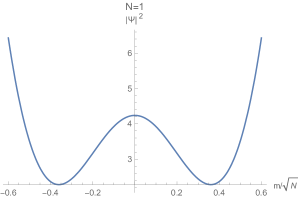
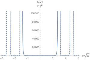
Figure 1: For a deformation corresponding to turning on a bulk pseudoscalar field, $|\Psi^{2}(m)|$ over a short and a long range at $N=1$. The point $m=0$ has been excluded from the short range plot due to problems with the numerical evaluation of very small numbers.

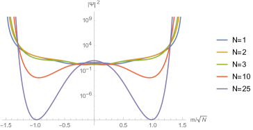
Figure 2: For a deformation corresponding to turning on a bulk pseudoscalar field, $|\Psi^{2}(m)|$.

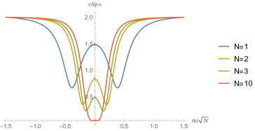
Figure 3: For a deformation corresponding to turning on a bulk pseudoscalar field, $N_{F}(m)$.

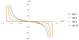
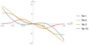
Figure 4: For a deformation corresponding to turning on a bulk pseudoscalar field, $<\tilde{\lambda}\lambda>[m]$.

The behaviour of $|\Psi|^{2}$ can be seen in figs. 1 and 2. We see that undeformed de Sitter space is a local maximum of $|\Psi|^{2}$, indicating the perturbative stability of the supersymmetric de Sitter vacuum. For very large deformations, we see divergences in $|\Psi|^{2}$. These divergences do not come as a surprise. They are not a result of the inclusion of the gauginos, they are already present when one considers the bulk pseudoscalar field by itself, as we already discussed in Hertog:2017ymy . In fact, we should restrict the outermost edge of the configuration space at which our results can be hoped to be trusted to $|m/\sqrt{N}|<3/2$ and we restrict our analysis of observables to this range. We defer the discussion of the reason for this restriction to section V.4

In fig. 3 the value of $<N_{F}>[m]$ can be seen. We shall interpret its behaviour and compare it to earlier bulk results in section V.4.

In fig. 4, $<\tilde{\lambda}\lambda>[m]$ can be seen. We see that it increases as we increase $|m|$. We also see that for $m/\sqrt{N}$ between $-3/2$ and $3/2$, it is antisymmetric, while $|\Psi|^{2}$ is symmetric in $m$. While we do not know the exact measure against which we should integrate the bosonic fields in the wave function, it seems reasonable that it should respect such symmetries. If this is the case, $<\tilde{\lambda}\lambda>=0$ for the holographic no-boundary wave function after integration over $m$.

V.2 Bulk scalar

For a deformation based on turning on a bulk scalar, the action at $N=1$ takes the form

$$S=\int d^{3}x\sqrt{h}\left[\begin{array}[]{c|c}\tilde{\chi}&\tilde{\varphi}\end{array}\right]\left[\begin{array}[]{c|c}{\rm i}\not{\nabla}&-\sqrt{2}{\rm i}\tilde{\lambda}\\ \hline\cr\sqrt{2}{\rm i}\lambda&-\partial^{2}+3/4+\sigma\end{array}\right]\left[\begin{array}[]{c}\chi\\ \hline\cr\varphi\end{array}\right]\text{,}$$ (42)

To compute the partition function

$$Z\propto\prod_{n}a_{n}^{-1}=\beta\,\gamma~{},~{}~{}~{}\beta:=\prod_{n}\frac{(\Lambda_{n})^{3}+\sigma\Lambda_{n}}{(\Lambda_{n})^{3}+\sigma\Lambda_{n}-2\tilde{\lambda\lambda}}~{},~{}~{}~{}\gamma:=\text{det}(-\partial^{2}+3/4+\sigma)\prod_{n}\frac{1}{(\Lambda_{n})}~{},~{}~{}~{}~{}~{}~{}$$ (43)

we proceed in the same way as the previous cases. Note that in this case, the $det(D)^{-1}$ term in eq. 25 is not constant, but depends on $\sigma$, so we must take it into account. We find for $N=1$

$$\beta =1-\frac{\pi\text{sech}^{2}\left(\pi\sqrt{\sigma}\right)\left(8\pi\sigma^{3/2}+4\pi\sqrt{\sigma}-(4\sigma+3)\sinh\left(2\pi\sqrt{\sigma}\right)+2\pi\sqrt{\sigma}\cosh\left(2\pi\sqrt{\sigma}\right)\right)}{32\sigma^{5/2}}(2\tilde{\lambda}\lambda)^{2}\,,$$ (44)

and

$$\gamma\propto\exp\Bigg{\{}-\frac{1}{24\pi^{2}}\bigg{[} \,\pi^{2}\left({\rm i}\pi\left(4\sigma\sqrt{1-4\sigma}-\sqrt{1-4\sigma}+1\right)+6(4\sigma-1)\log\left(1-e^{-{\rm i}\pi\sqrt{1-4\sigma}}\right)\right)$$

$$-12{\rm i}\pi\sqrt{1-4\sigma}\text{Li}_{2}\left(e^{-{\rm i}\sqrt{1-4\sigma}\pi}\right)-12\text{Li}_{3}\left(e^{-{\rm i}\sqrt{1-4\sigma}\pi}\right)\bigg{]}\Bigg{\}}\,.$$ (45)

We again expand $\beta$ via the methods described previously. In this case, it was possible to find $\beta$ analytically. It is worth noting that $\sum_{n}a_{n}=0$. Looking at eq. 35, this ensures that in the large $N$ limit, the parts of the wave function with bulk fermions excited are supressed and the local fermion excitation number tends to zero. Of course, any actual divergences introduced by the gauginos remain at any finite $N$.

Without the gauginos but with only the scalar mass deformation, our deformation would be essentially equivalent to the scalar deformation considered at the start of Anninos:2012ft . As such, it makes sense to compare this wave function to the one discussed there. For $N=1$, $|\Psi|^{2}$ can be seen in fig. 5. We see that for small deformation, there is a local maximum for $|\Psi|^{2}$ at undeformed de Sitter space. For positive deformations, this maximum is global. For negative deformations, we see large fluctuations, as were also found in Anninos:2012ft . Here the problem seems to be exacerbated. Rather than large finite fluctuations, $|\Psi|^{2}$ now only diverges for sufficiently large negative deformations, with the first divergency at $\sigma/\sqrt{N}=-9/4$. As we shall discuss in section V.4, we should restrict the configuration space to $\sigma/\sqrt{N}>-3/4$.

The fermion number can be seen in fig. 6, we postpone its analysis to section V.4. We see that $<\tilde{\lambda}\lambda>=0$ as there is no first order term in $\tilde{\lambda}\lambda$ in the wave function.

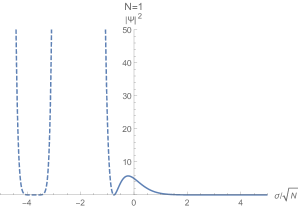
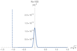
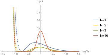
Figure 5: For a deformation corresponding to turning on a bulk scalar field, $|\Psi^{2}(\sigma)|$.

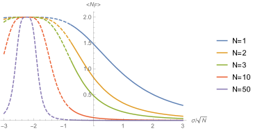
Figure 6: For a deformation corresponding to turning on a bulk scalar field, $N_{F}(\sigma)$.

V.3 Squashing

Finally, we combine the spin-1/2 deformation with a squashing of the three-sphere. The action takes the form

$$S=\int d^{3}x\sqrt{h_{\text{def}}}\left[\begin{array}[]{c|c}\tilde{\chi}&\tilde{\varphi}\end{array}\right]\left[\begin{array}[]{c|c}{\rm i}\not{\nabla}&-\sqrt{\frac{2}{N}}{\rm i}\tilde{\lambda}\\ \hline\cr\sqrt{\frac{2}{N}}{\rm i}\lambda&-\partial^{2}+\frac{R}{8}\end{array}\right]\left[\begin{array}[]{c}\chi\\ \hline\cr\varphi\end{array}\right]\text{.}$$ (46)

Turning on the squashing changes the eigenvalues of the Dirac operator and Laplacian. We consider a squashing preserving $SU(2)\times U(1)$ symmetry described by the metric

$$ds_{S^{3}_{\alpha}}^{2}=d\theta^{2}+\sin^{2}\theta d\phi^{2}\,+\frac{1}{1+\alpha}(d\tilde{\psi}+\cos\theta d\phi)^{2}\,,$$ (47)

where $\theta\in[0,\pi]$, $\phi\in[0,2\pi]$, $\tilde{\psi}\in[0,4\pi]$, and the real deformation parameter $\alpha$ is such that $\alpha>-1$.

The eigenvalues of the Dirac operator are of the form Bobev:2017asb ; Dowker:1998pi ; Gibbons:1979kq ; HITCHIN19741

$$\Lambda_{n,q,\,\pm}=\frac{1}{2\sqrt{1+\alpha}}\pm 2\sqrt{\frac{n^{2}(1+\alpha)}{4}-\alpha q(n-q)}\,,$$ (48)

with degeneracy $n$. Here the eigenvalues run over two branches. For the positive branch, $n=1,..,\infty$ and $q=0,..,n$ while for the negative branch, $n=2,..,\infty$ and $q=1,..,n-1$. To compute the partition function, the same logic as in the previous sections applies, except that we use the eigenvalues of the Dirac operator on the squashed three-sphere. We find for $N=1$

$$\beta=\prod_{n,q}\frac{\Lambda_{n,q}^{3}}{\Lambda_{n,q}^{3}-2\tilde{\lambda}\lambda}\,.$$ (49)

The gaugino independent part of the partition function, $\gamma$, is the partition function for a free spinor and complex scalar on a squashed three sphere. This was computed numerically in Bobev:2017asb where a good agreement was found between the numerical result and the following analytic expression which we will use for $\gamma$,

$$\gamma=-(-1)^{23/24}\sqrt[4]{2}e^{\frac{3\zeta(3)}{4\pi^{2}}-\frac{\pi^{2}\alpha^{2}}{16(\alpha+1)^{2}}}\,.$$ (50)

We compute $\beta$ numerically, analogously to the previous sections, in this way obtain $Z=\beta\gamma$ and identify it with the wave function under dS/CFT.

The behaviour of $|\Psi|^{2}$ under squashing can be seen in fig. 7. We find an interesting dependence on $N$. At small $N$, $|\Psi|^{2}$ is peaked for a squashed three-sphere. As $N$ increases, we see that the peak of $|\Psi|^{2}$ quickly moves back to te undeformed three-sphere. At large $N$, $|\Psi|^{2}$ has a global maximum at undeformed de Sitter space, indicating the stability of the de Sitter vacuum. At small $N$, the stable vacuum around which one should consider perturbation theory seems to be squashed away from the three-sphere. For reasons discussed in section V.4, we should restrict the configuration space to $\alpha>-3/4$

The fermion occupation number, whose properties we will discuss further in section V.4, can be seen in fig. 8. In fig. 9, $<\tilde{\lambda}\lambda>[B]$ can be seen. We see that it is negative and reaches an extremum at finite squashing.

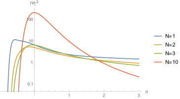
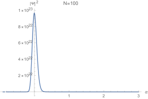
Figure 7: For a squashing, $|\Psi(\alpha)|^{2}$ .

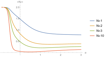
Figure 8: For a squashing, $N_{F}(\alpha)$.

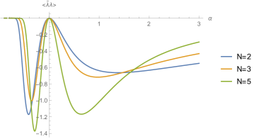
Figure 9: For a squashing, $<\tilde{\lambda}\lambda>$ .

V.4 Interpretation and Comparison

Deformation	Effect on wavefunction	Studied in
Scalar	Perturbatively stable around empty de Sitter	Anninos:2012ft
BPS scalar + pseudoscalar	Perturbatively stable around empty de Sitter	Hertog:2017ymy
BPS vector + metric squashing	Perturbatively stable around empty de Sitter	Hertog:2017ymy
Spinor	Fermion states occupied at small $N$, unoccupied at large $N$	section IV
Spinor + pseudoscalar	Perturbatively stable around empty de Sitter	section V.1
Spinor + scalar	Perturbatively stable, peak shifted from empty dS at small $N$	section V.2
Spinor + metric squashing	Perturbatively stable, peak shifted from empty dS at small $N$	section V.3

Table 1: Summary of for which bulk fields the wavefunction of the $\mathcal{N}=2$ supersymmetric higher spin theory has been computed using dS/CFT. The pseudoscalar field or squashing by itself in the SUSY model have not been given a detailed discussion, but its behaviour can easily be seen by setting $\beta=1$ in the relevant section.

We have computed the Hartle - Hawking wave function for an asymptotically nearly de Sitter universe in a ‘minisuperspace’ model consisting of the zero mode of a spin-1/2 field, a pseudoscalar, a scalar and a metric deformation as excitations around dS space. A summary of the deformations studied in this paper and the earlier literature can be seen in table 1. The wave function predicts probabilities for different asymptotic configurations (or more precisely, different spacetime histories). The figs. 1, 2, 5 and 7 show that the probability distributions exhibit a local maximum for reasonably small deformations in all directions of the minisuperspace. At small $N$, this maximum can be shifted somewhat away from the undeformed dS configuration. At large $N$, however, it always lies perfectly at the empty, undeformed de Sitter space. In this semiclassical limit the wave function becomes increasingly sharply concentrated around this configuration. The presence of a local maximum at empty dS also indicates that dS is perturbatively stable. The behaviour of the wave function for small fluctuations around dS describes correlators of fields in dS, and a maximum ensures these behave correctly.

For integer-spin sources, the fact that the probabilities are peaked at empty undeformed de Sitter space follows basically from an analytic continuation of the F-theorem Jafferis:2010un ; Jafferis:2011zi ; Klebanov2011 ; Casini:2012ei . This states that for unitary QFTs on $S^{3}$, the free energy is maximized by a UV CFT and any deformation - including complex deformations - decreases it. This theorem has been proven and extended to a variety of CFT deformations, e.g. the extension in Bobev:2017asb is especially relevant for us. With the spin-1/2 source deformation included, it is at small $N$ no longer true that the wave function squared is peaked at empty undeformed de Sitter space. It is also not clear whether the wave function has a meaningful interpretation in terms of probabilities in this limit. In fact, with a spin-1/2 source, the partition function is supernumber-valued and there is no longer an unambiguous notion of maximum for $Z$. First, $Z$ must be mapped to the real numbers to speak of maximization. The inner product eq. 7 provides such a map, but there is no reason why an F-theorem should imply maximization at the undeformed CFT with respect to this specific inner product. Still, there is a notion of $Z$ being extremized with respect to the spin-1/2 deformation at the undeformed CFT. Clearly the first derivative of eq. 32 with respect to $\lambda$, $\tilde{\lambda}$, or both, is zero at $\lambda=0$ or $\tilde{\lambda}=0$. This implies that $<\tilde{\lambda}\lambda>=0$.

For large scalar or pseudoscalar deformations our results may give the impression that the probabilities exhibit divergences. However, as we already mentioned in section V, dS/CFT comes with a significant restriction on the configuration space of deformations which in particular excludes the regime where we find the wave function diverges. These restrictions are indicated with a transition to dotted lines in the figures above.

For the scalar deformation, we can identify the boundaries of the configuration space with a good degree of confidence. Here, the completion of dS/CFT of Anninos:2017eib which provides not just a wave function but also a Hilbert space and an inner product, directly applies to our model. It implies a measure that restricts the configuration space of the wave function to deformations with $\sigma/\sqrt{N}>-3/4$. In Hertog:2017ymy we gave an independent argument for the same bound based on the origin of dS/CFT as a continuation of Euclidean AdS/CFT. At $\sigma/\sqrt{N}=-3/4$ one of the eigenvalues of the dynamical CFT scalar becomes zero, and below this it becomes negative. As a result, the (super)gaussian formula for the partition function path integral no longer applies. Instead the EAdS dual partition function is manifestly divergent for $\sigma/\sqrt{N}<-3/4$ and thus predicts a vanishing wave function in this domain Hertog2011 ; Conti:2017pqc . Similar arguments apply to the metric deformations we considered; the dynamical CFT scalar has zero or negative eigenvalues for squashings $\alpha\leq-3/4$ leading to a vanishing wave function in this regime Conti:2017pqc .

Finally, for the pseudoscalar deformation, the situation is less clear. The pseudoscalar deformation only affects the eigenvalues of the dynamical CFT spinor, not those of the scalar. Spinors always have negative eigenvalues and these do not pose a problem for the path integral. However, trouble does appear when there are spinor zero eigenmodes resulting in a divergent wave function. The first of these appear when $|m/\sqrt{N}|=3/2$ and thus our results should at most be trusted for $|m/\sqrt{N}|<3/2$. It would be very interesting to obtain a better understanding of the measure against which the wave function should be evaluated for pseudoscalar bulk fields. To give a spark of hope that the zero-eigenmode divergencies can in due time be dealt with, we point out that an analogous problem appears in the RNS quantization of the superstring. Here, commuting spinor ghosts $\beta$ and $\gamma$ are introduced Polchinski:1998rr . These have a number of zero eigenmodes depending on the genus of the worldsheet one consider which produce formal divergencies in the computations, but it is understood how the theory must be modified to resolve these.

For a pseudoscalar bulk deformation, the value of $<N_{F}>[m]$ can be seen in fig. 3. We stress again that, as discussed in section II, this object has been constructed to compute the fermion occupation number at a given value of the bulk scalar, with the latter treated as an external condensate. At large $N$, we see that $N_{F}$ is zero at $m=0$, that it increases with increasing $|m|$, saturating at complete occupation at $|m/\sqrt{N}|=3/2$. This agrees beautifully with the earlier bulk computations of DEath:1986lxx ; DEath:1996ejf as follows: We do not know the bulk action when one integrates out all degrees of freedom, retaining only the bulk pseudoscalar and spin-1/2 field. Still, generically, the leading coupling between a scalar and a spinor is of the Yukawa-type. In the presence of a non-dynamical external scalar field, the Yukawa coupling effectively acts as a mass term for the spinor. We expect the large $N$ limit in the CFT to correspond to the free limit since $N=(G_{N}\Lambda)^{-1}$ and we work at constant $\Lambda$. One then expects that for a boundary source $m/\sqrt{N}$ and at large $N$, the bulk fermion will effectively behave as a free massive spin-1/2 fermion of mass $m_{F}=m/\sqrt{N}$. In DEath:1986lxx ; DEath:1996ejf the Hartle-Hawking wave function, together with $<N_{F}>[m_{F}]$, was computed for a free fermion in Einstein gravity in de Sitter space. For a massless bulk fermion, they found that $N_{F}$ should be zero. Next, $N_{F}$ should increase with increasing $|m_{F}|$. For modes with $n+3/2\ll|m_{F}|$ at $l=1$, they found that $N_{F}$ should saturate at maximum occupation. We are looking at constant spinors with $n=0$, so this completely agrees with our boundary result, within the range of $|m_{F}|$ where our analysis is to be trusted.

The interplay of the spin-1/2 field with the bulk scalar differs from that with the pseudoscalar, especially in the large $N$ limit. Since $\sum_{n}a_{n}=0$, in the scalar case the part of the wave function with spin-1/2 states excited totally disappears here; it appears the scalar and spin-1/2 field do not interact in the large $N$ limit. This may be a consequence of the boundary conditions we employ. The deformations of the boundary CFT correspond to the standard quantisation for the bulk pseudoscalar and to the alternate quantization for the bulk scalar Hertog:2017ymy . It would be interesting to explore whether the interplay between the bulk bosons and the spin-1/2 field changes for different boundary conditions.

VI Outlook

We have initiated the study of fermionic bulk fields in dS/CFT, working with the dualities relating ${\cal N}=2$ supersymmetric Euclidean vector models with reversed spin-statistics in three dimensions to supersymmetric Vasiliev theories in four-dimensional de Sitter space. Specifically we have holographically evaluated the Hartle - Hawking wave function in the bulk in a number of homogeneous minisuperspace models consisting of a half-integer spin field coupled to a scalar, a pseudoscalar or a metric squashing. With a well-motivated measure we have found the wave function to be normalizable and globally peaked at or near the supersymmetric de Sitter vacuum, with a low amplitude for large deformations. A detailed discussion of its behavior and a comparison with earlier bulk computations in the semiclassical limit is given in Section V.4 above.

We have considered the lowest, homogeneous mode of a spin-1/2 bulk field only. It would be natural to look at higher modes, and to study bulk fermions of higher spin. Gravitinos have been studied in a supergravity context in AdS/CFT and in supersymmetric quantum cosmology Corley:1998qg ; Volovich:1998tj ; DEath:1988jyp ; DEath:1992wve ; Moniz:1996pd . Beyond this, higher spin theories have an infinite tower of fermionic higher spin fields. The expressions for the conserved CFT currents related to these fields are known exactly Nizami:2013tpa . Since it is relatively straightforward to compute the wave function for fermionic bulk fields (compared to bosonic fields) one might hope to compute the wave function for the lowest modes of these fermionic higher spin fields exactly.

We have seen that the fermionic contributions introduce an interesting $N$-dependence in the theory. dS/CFT at finite $N$ is largely unexplored territory, but recently the Q-model Anninos:2017eib ; Anninos:2019nib has been put forward as a possible completion of higher-spin dS/CFT. We made use of the measure implied by the Q-model to identify the domain of the wave function in some of the models we considered in this paper. An interesting avenue for future research would be to examine whether fermionic bulk fields can be implemented in the Q-model and to explore how various small $N$ effects play out against each other.

Other possible generalizations in the HS context include the study of fermions in the causal patch version of dS/CFT, currently formulated in terms of a boundary particle mechanics Neiman:2018ufb , and in FLRW-like cosmologies in higher spin theory Aros:2017ror for which currently a dual description has yet to be found.

Undoubtedly the most challenging open question concerns the formulation of a precise dS/CFT duality in string theory. One important difference with HS theory, when it comes to dS/CFT, is that string theory has towers of fields of arbitrarily high mass whereas HS theory contains only massless and very light fields. It is well known that light scalar fields in dS with masses below the dS analogue $m^{2}_{BF}=9/4H^{2}$ of the Breitenlohner - Freedman (BF) bound behave very differently from more massive fields Strominger:2001pn ; McInnes:2001dq ; Hartle:2008ng ; Kiritsis:2019wyk ; Thomastalk . It is worth noting in this context that the semiclassical Hartle - Hawking wave function vanishes in dynamical models of de Sitter gravity coupled to massive scalars with masses $m^{2}>m^{2}_{BF}$, at least for reasonably small deformations of de Sitter Hartle2007 . This suggests that if it computes the Hartle - Hawking wave function, dS/CFT duality should incorporate a final condition on such massive scalars that sets these to zero. This is effectively what we have seen in the minisuperspace models we have analysed, as discussed in Section V.4 above, and this would resolve the tension between dS/CFT and the swampland arguments Brennan:2017rbf ; Danielsson:2018ztv ; Garg:2018reu ; Obied:2018sgi ; Ooguri:2018wrx ; Andriot:2018ept , some of which suggesting dS with $m^{2}>m^{2}_{BF}$ scalars is unstable.

Finally, it is tempting to speculate that our findings are connected to the supersymmetric dS constructions in exotic string theories Hull:1998vg . The latter have vector ghosts in their supergravity limits related to the existence of non-compact $R$-symmetry groups in their representation of the algebra. However Hull has argued that the massive string states in exotic string theories may well render the de Sitter vacua ghost-free and unitary. In Hertog:2017ymy we conjectured that the supersymmetric higher-spin theories in dS that we construct are related indeed to the tensionless limit of these exotic string theories. It would be very interesting to explore the extension to dS/CFT of the ABJ triality Chang:2012kt linking higher spin theory and string theory in AdS/CFT from a complementary angle and in different regimes.

Appendix A Quantization fermions in de Sitter space

In this appendix we provide some additional details on the quantization of a free massless spinor in four-dimensional de Sitter space and the definition of $\breve{\psi}$. None of these results are new, we merely summarize some results of DEath:1986lxx ; DEath:1996ejf without derivation, specialized to the case of a massless two-component spinor and add to this some comments related to higher spin theory. The interested reader can find a more complete treatment in those texts, including also the extension to a massive dirac spinor and the inclusion of dynamical metric and scalar fields. We will consider the metric for a spacetime whose spatial slices are three-spheres,

$$ds^{2}=-dt^{2}+e^{2\alpha(t)}d\Omega_{3}^{2}\,,$$ (51)

with $d\Omega_{3}^{2}$ the metric on the unit three-sphere. We will denote the metric on a spatial slice by $h_{ij}(t)$. When $e^{\alpha(t)}\simeq l\text{ cosh}(t/l)$, one is approximately in a de Sitter regime, with de Sitter radius $l$. One could demand this behaviour for the entire spacetime or asymptotically at late times as desired. Our discussion will be valid for generic metrics of the form eq. 51.

The standard action for a two-component massless spinor $\psi^{A}$ in tertad $e^{a}_{\mu}$ and bispinor for tangent vector $a\rightarrow AA^{\prime}$ notation has the volume term

$$I_{V}=-\frac{{\rm i}}{2}\int d^{4}x\,e\,\breve{\psi}^{A^{\prime}}e^{\mu}_{AA^{\prime}}D_{\mu}\psi^{A}\,.$$ (52)

Here $\breve{\psi}^{A^{\prime}}$ is ordinarily the Dirac adjoint $\overline{\psi}^{A^{\prime}}=(\psi^{A})^{\dagger}$ of $\psi^{A}$ (but read on!). We follow DEath:1986lxx ; DEath:1996ejf in introducing a seperate notation to indicate that for, e.g., the purpose of varying the action, computing conjugate momenta, canonically quantizing in an Hamiltinioan approach, one treats $\psi^{A}$ and $\breve{\psi}^{A^{\prime}}$ as if they were independent. This is the standard textbook approach, though the notation is nonstandard.

Following this breve notation provides one further advantage in our case. In the supersymmetric de Sitter higher spin theory of Sezgin:2012ag , which forms the bulk side of the specific dS/CFT duality treated in this paper, there appears a conjugate, which we will denote with $c$, which acts as the hermitian conjugate $\dagger$ on bosonic quantities. On fermionic quantities, however, it has the special property that $((\psi^{A})^{c})^{c}=-\psi^{A}$. Conjugate spinors in the higher spin theory are defined using this $c$ conjugate rather than the hermitian conjugate. Because we treat $\psi^{A}$ and $\breve{\psi}^{A^{\prime}}$ as if they were independent, we can treat the cases $\breve{\psi}^{A^{\prime}}=(\psi^{A})^{\dagger}$ and $\breve{\psi}^{A^{\prime}}=(\psi^{A})^{c}$ at the same time and the need to distinguish the two will not come up in this appendix or section II. We can thus discuss the general framework for including fermions in dS/CFT in both ordinary gravity + matter theories and higher spin theories at the same time.

In the presence of an initial $\Sigma_{I}$ and/or final $\Sigma_{F}$ boundary surface, the action also requires boundary terms

$$I_{B}=\frac{{\rm i}}{2}\left(\int_{\Sigma_{I}}+\int_{\Sigma_{F}}\right)d^{3}x\,h^{1/2}\,\breve{\psi}^{A^{\prime}}n_{AA^{\prime}}\psi^{A}\,,$$ (53)

with $n^{AA^{\prime}}$ the unit timelike vector normal to the surface. The conjugate momentum to $\psi^{A}$ is given by

$$\pi_{A}=-\frac{{\rm i}}{2}h^{1/2}n_{AA^{\prime}}\breve{\psi}^{A^{\prime}}\,.$$ (54)

Using this identity, we can and will take the fundamental dynamical variables of the theory to be $\psi^{A}$ and $\breve{\psi}^{A}$ rather than $\psi^{A}$ and $\pi_{A}$.

One finds the classical Dirac bracket

$$\{h^{1/4}\psi^{A}(x)\,,h^{1/4}\breve{\psi}^{A^{\prime}}(x^{\prime})\}_{D}=-2{\rm i}n^{AA^{\prime}}\delta(x,x^{\prime})\,,$$ (55)

and all other Dirac brackets zero. One quantizes by the usual procedure, turning the Dirac brackets into anticommutators with factor of ${\rm i}\hbar$ inserted. One can expand spinor-valued functions in the background of eq. 51 in spatial three-sphere harmonics. We denote the positive frequency three-sphere harmonics by $\rho^{np}_{A}$ and $\sigma^{np}_{A^{\prime}}$; the negative frequency harmonics by $\overline{\rho}^{np}_{A^{\prime}}$ and $\overline{\sigma}^{np}_{A}$. The indices run over $n=0,1,2,...$ and $p=1,2,..,(n+1)(n+2)$. The expansions of $\psi^{A}$ and $\breve{\psi}^{A^{\prime}}$ are then given by

$$\psi_{A} =\frac{e^{-3\alpha/2}}{2\pi}\sum_{n}\sum_{p}\big{(}s_{np}(t)\rho^{np}_{A}+\breve{t}_{np}(t)\overline{\sigma}^{np}_{A}\big{)}\,,$$ (56a)

$$\breve{\psi}_{A^{\prime}} =\frac{e^{-3\alpha/2}}{2\pi}\sum_{n}\sum_{p}\big{(}\breve{s}_{np}(t)\overline{\rho}^{np}_{A^{\prime}}+t_{np}(t)\sigma^{np}_{A^{\prime}}\big{)}\,.$$ (56b)

The dynamical coeffecients $s_{np}(t)$, $\breve{t}_{np}(t)$, $\breve{s}_{np}(t)$, $t_{np}(t)$ are Grassmann-valued for anticommuting spinors, as is the case here. The prefactors in front of these expansions could equally well have been absorbed into the dynamical coefficients. This choice of prefactors is convenient as they counteract the factors of $h^{1/4}$ appearing in eq. 55. This ensures that upon quantization one obtains eq. 3b without any further factors or metric dependence.

References

- (1) C. M. Hull, “Timelike T duality, de Sitter space, large N gauge theories and topological field theory,” JHEP 07 (1998) 021, arXiv:hep-th/9806146 [hep-th].
- (2) V. Balasubramanian, J. de Boer, and D. Minic, “Mass, entropy and holography in asymptotically de Sitter spaces,” Phys.Rev. D65 (2002) 123508, arXiv:hep-th/0110108 [hep-th].
- (3) A. Strominger, “The dS / CFT correspondence,” JHEP 10 (2001) 034, arXiv:hep-th/0106113 [hep-th].
- (4) J. B. Hartle and S. W. Hawking, “Wave Function of the Universe,” Phys. Rev. D28 (1983) 2960–2975.
- (5) J. M. Maldacena, “Non-Gaussian features of primordial fluctuations in single field inflationary models,” JHEP 05 (2003) 013, arXiv:astro-ph/0210603 [astro-ph].
- (6) D. Harlow and D. Stanford, “Operator Dictionaries and Wave Functions in AdS/CFT and dS/CFT,” arXiv:1104.2621 [hep-th].
- (7) J. Maldacena, “Einstein Gravity from Conformal Gravity,” arXiv:1105.5632 [hep-th].
- (8) T. Hertog and J. Hartle, “Holographic No-Boundary Measure,” JHEP 1205 (2012) 095, arXiv:1111.6090 [hep-th].
- (9) D. Anninos, T. Hartman, and A. Strominger, “Higher Spin Realization of the dS/CFT Correspondence,” Class. Quant. Grav. 34 no. 1, (2017) 015009, arXiv:1108.5735 [hep-th].
- (10) R. Dijkgraaf, B. Heidenreich, P. Jefferson, and C. Vafa, “Negative Branes, Supergroups and the Signature of Spacetime,” JHEP 02 (2018) 050, arXiv:1603.05665 [hep-th].
- (11) K. Skenderis, P. K. Townsend, and A. Van Proeyen, “Domain-wall/cosmology correspondence in adS/dS supergravity,” JHEP 08 (2007) 036, arXiv:0704.3918 [hep-th].
- (12) E. A. Bergshoeff, J. Hartong, A. Ploegh, J. Rosseel, and D. Van den Bleeken, “Pseudo-supersymmetry and a tale of alternate realities,” JHEP 07 (2007) 067, arXiv:0704.3559 [hep-th].
- (13) J. B. Hartle, S. Hawking, and T. Hertog, “Quantum Probabilities for Inflation from Holography,” JCAP 1401 no. 01, (2014) 015, arXiv:1207.6653 [hep-th].
- (14) D. Anninos, F. Denef, and D. Harlow, “Wave function of Vasiliev’s universe: A few slices thereof,” Phys. Rev. D88 no. 8, (2013) 084049, arXiv:1207.5517 [hep-th].
- (15) D. Anninos, F. Denef, G. Konstantinidis, and E. Shaghoulian, “Higher Spin de Sitter Holography from Functional Determinants,” JHEP 02 (2014) 007, arXiv:1305.6321 [hep-th].
- (16) N. Bobev, T. Hertog, and Y. Vreys, “The NUTs and Bolts of Squashed Holography,” JHEP 11 (2016) 140, arXiv:1610.01497 [hep-th].
- (17) G. Conti, T. Hertog, and Y. Vreys, “Squashed Holography with Scalar Condensates,” JHEP 09 (2018) 068, arXiv:1707.09663 [hep-th].
- (18) S. W. Hawking and T. Hertog, “A Smooth Exit from Eternal Inflation?,” JHEP 04 (2018) 147, arXiv:1707.07702 [hep-th].
- (19) M. A. Vasiliev, “Consistent equation for interacting gauge fields of all spins in (3+1)-dimensions,” Phys. Lett. B243 (1990) 378–382.
- (20) I. R. Klebanov and A. M. Polyakov, “AdS dual of the critical O(N) vector model,” Phys. Lett. B550 (2002) 213–219, arXiv:hep-th/0210114 [hep-th].
- (21) S. Giombi, “Higher Spin — CFT Duality,” in Proceedings, Theoretical Advanced Study Institute in Elementary Particle Physics: New Frontiers in Fields and Strings (TASI 2015): Boulder, CO, USA, June 1-26, 2015, pp. 137–214. 2017. arXiv:1607.02967 [hep-th].
- (22) T. Hertog, G. Tartaglino-Mazzucchelli, T. Van Riet, and G. Venken, “Supersymmetric dS/CFT,” JHEP 02 (2018) 024, arXiv:1709.06024 [hep-th].
- (23) K. Pilch, P. van Nieuwenhuizen, and M. F. Sohnius, “De Sitter Superalgebras and Supergravity,” Commun. Math. Phys. 98 (1985) 105.
- (24) J. Lukierski and A. Nowicki, “All Possible De Sitter Superalgebras and the Presence of Ghosts,” Phys. Lett. 151B (1985) 382–386.
- (25) E. Witten, “Quantum gravity in de Sitter space,” in Strings 2001: International Conference Mumbai, India, January 5-10, 2001. 2001. arXiv:hep-th/0106109 [hep-th].
- (26) E. Sezgin and P. Sundell, “Supersymmetric Higher Spin Theories,” J. Phys. A46 (2013) 214022, arXiv:1208.6019 [hep-th].
- (27) G. W. Gibbons and S. W. Hawking, “Cosmological Event Horizons, Thermodynamics, and Particle Creation,” Phys. Rev. D15 (1977) 2738–2751.
- (28) T. Anous, D. Z. Freedman, and A. Maloney, “de Sitter Supersymmetry Revisited,” JHEP 07 (2014) 119, arXiv:1403.5038 [hep-th].
- (29) M. Buican and Z. Laczko, “Nonunitary Lagrangians and unitary non-Lagrangian conformal field theories,” Phys. Rev. Lett. 120 no. 8, (2018) 081601, arXiv:1711.09949 [hep-th].
- (30) M. Buican and Z. Laczko, “Rationalizing CFTs and Anyonic Imprints on Higgs Branches,” JHEP 03 (2019) 025, arXiv:1901.07591 [hep-th].
- (31) P. D. D’Eath and J. J. Halliwell, “Fermions in Quantum Cosmology,” Phys. Rev. D35 (1987) 1100.
- (32) P. D. D’Eath, Supersymmetric quantum cosmology. Cambridge Monographs on Mathematical Physics. Cambridge University Press, 2011.
- (33) M. F. Atiyah, V. K. Patodi, and I. M. Singer, “Spectral asymmetry and Riemannian Geometry 1,” Math. Proc. Cambridge Phil. Soc. 77 (1975) 43.
- (34) F. A. Berezin, “The method of second quantization,” Pure Appl. Phys. 24 (1966) 1–228.
- (35) L. D. Faddeev and A. A. Slavnov, “GAUGE FIELDS. INTRODUCTION TO QUANTUM THEORY,” Front. Phys. 50 (1980) 1–232. [Front. Phys.,1(1991)].
- (36) B. Willett, “Localization on three-dimensional manifolds,” J. Phys. A50 no. 44, (2017) 443006, arXiv:1608.02958 [hep-th].
- (37) S. M. Kuzenko, U. Lindström, and G. Tartaglino-Mazzucchelli, “Off-shell supergravity-matter couplings in three dimensions,” JHEP 03 (2011) 120, arXiv:1101.4013 [hep-th].
- (38) S. M. Kuzenko and G. Tartaglino-Mazzucchelli, “Three-dimensional N=2 (AdS) supergravity and associated supercurrents,” JHEP 12 (2011) 052, arXiv:1109.0496 [hep-th].
- (39) E. Sezgin and P. Sundell, “Massless higher spins and holography,” Nucl. Phys. B644 (2002) 303–370, arXiv:hep-th/0205131 [hep-th]. [Erratum: Nucl. Phys.B660,403(2003)].
- (40) R. G. Leigh and A. C. Petkou, “Holography of the N=1 higher spin theory on AdS(4),” JHEP 06 (2003) 011, arXiv:hep-th/0304217 [hep-th].
- (41) E. Sezgin and P. Sundell, “Holography in 4D (super) higher spin theories and a test via cubic scalar couplings,” JHEP 07 (2005) 044, arXiv:hep-th/0305040 [hep-th].
- (42) N. Bobev, P. Bueno, and Y. Vreys, “Comments on Squashed-sphere Partition Functions,” JHEP 07 (2017) 093, arXiv:1705.00292 [hep-th].
- (43) J. S. Dowker, “Effective actions on the squashed three sphere,” Class. Quant. Grav. 16 (1999) 1937–1953, arXiv:hep-th/9812202 [hep-th].
- (44) G. W. Gibbons, “Spectral Asymmetry and Quantum Field Theory in Curved Space-time,” Annals Phys. 125 (1980) 98. [,471(1979)].
- (45) N. Hitchin, “Harmonic spinors,” Advances in Mathematics 14 no. 1, (1974) 1 – 55.
- (46) D. L. Jafferis, “The Exact Superconformal R-Symmetry Extremizes Z,” JHEP 05 (2012) 159, arXiv:1012.3210 [hep-th].
- (47) D. L. Jafferis, I. R. Klebanov, S. S. Pufu, and B. R. Safdi, “Towards the F-Theorem: N=2 Field Theories on the Three-Sphere,” JHEP 06 (2011) 102, arXiv:1103.1181 [hep-th].
- (48) I. R. Klebanov, S. S. Pufu, and B. R. Safdi, “F-Theorem without Supersymmetry,” JHEP 1110 (2011) 038, arXiv:1105.4598 [hep-th].
- (49) H. Casini and M. Huerta, “On the RG running of the entanglement entropy of a circle,” Phys. Rev. D85 (2012) 125016, arXiv:1202.5650 [hep-th].
- (50) D. Anninos, F. Denef, R. Monten, and Z. Sun, “Higher Spin de Sitter Hilbert Space,” arXiv:1711.10037 [hep-th].
- (51) J. Polchinski, String theory. Vol. 2: Superstring theory and beyond. Cambridge Monographs on Mathematical Physics. Cambridge University Press, 2007.
- (52) S. Corley, “The Massless gravitino and the AdS / CFT correspondence,” Phys. Rev. D59 (1999) 086003, arXiv:hep-th/9808184 [hep-th].
- (53) A. Volovich, “Rarita-Schwinger field in the AdS / CFT correspondence,” JHEP 09 (1998) 022, arXiv:hep-th/9809009 [hep-th].
- (54) P. D. D’Eath and D. I. Hughes, “SUPERSYMMETRIC MINISUPERSPACE,” Phys. Lett. B214 (1988) 498–502.
- (55) P. D. D’Eath and D. I. Hughes, “Minisuperspace with local supersymmetry,” Nucl. Phys. B378 (1992) 381–409.
- (56) P. V. Moniz, “Supersymmetric quantum cosmology: Shaken not stirred,” Int. J. Mod. Phys. A11 (1996) 4321–4382, arXiv:gr-qc/9604025 [gr-qc].
- (57) A. A. Nizami, T. Sharma, and V. Umesh, “Superspace formulation and correlation functions of 3d superconformal field theories,” JHEP 07 (2014) 022, arXiv:1308.4778 [hep-th].
- (58) E. I. Buchbinder, J. Hutomo, and S. M. Kuzenko, “Higher spin supercurrents in anti-de Sitter space,” JHEP 09 (2018) 027, arXiv:1805.08055 [hep-th].
- (59) J. Hutomo, S. M. Kuzenko, and D. Ogburn, “ supersymmetric higher spin gauge theories and current multiplets in three dimensions,” Phys. Rev. D98 no. 12, (2018) 125004, arXiv:1807.09098 [hep-th].
- (60) J. Hutomo and S. M. Kuzenko, “Higher spin supermultiplets in three dimensions: (2,0) AdS supersymmetry,” Phys. Lett. B787 (2018) 175–181, arXiv:1809.00802 [hep-th].
- (61) D. Anninos, V. De Luca, G. Franciolini, A. Kehagias, and A. Riotto, “Cosmological Shapes of Higher-Spin Gravity,” JCAP 2019 no. 04, (2019) 045, arXiv:1902.01251 [hep-th].
- (62) Y. Neiman, “Holographic quantization of linearized higher-spin gravity in the de Sitter causal patch,” JHEP 11 (2018) 033, arXiv:1809.07270 [hep-th].
- (63) R. Aros, C. Iazeolla, J. Noreña, E. Sezgin, P. Sundell, and Y. Yin, “FRW and domain walls in higher spin gravity,” JHEP 03 (2018) 153, arXiv:1712.02401 [hep-th].
- (64) B. McInnes, “Exploring the similarities of the dS / CFT and AdS / CFT correspondences,” Nucl. Phys. B627 (2002) 311–329, arXiv:hep-th/0110062 [hep-th].
- (65) J. B. Hartle, S. W. Hawking, and T. Hertog, “The Classical Universes of the No-Boundary Quantum State,” Phys. Rev. D77 (2008) 123537, arXiv:0803.1663 [hep-th].
- (66) E. Kiritsis and A. Tsouros, “de Sitter versus Anti de Sitter flows and the (super)gravity landscape,” arXiv:1901.04546 [hep-th].
- (67) T. Van Riet. Private communication, postings on Facebook and Twitter.
- (68) J. B. Hartle, S. Hawking, and T. Hertog, “No-Boundary Measure of the Universe,” Phys.Rev.Lett. 100 (2008) 201301, arXiv:0711.4630 [hep-th].
- (69) T. D. Brennan, F. Carta, and C. Vafa, “The String Landscape, the Swampland, and the Missing Corner,” PoS TASI2017 (2017) 015, arXiv:1711.00864 [hep-th].
- (70) U. H. Danielsson and T. Van Riet, “What if string theory has no de Sitter vacua?,” Int. J. Mod. Phys. D27 no. 12, (2018) 1830007, arXiv:1804.01120 [hep-th].
- (71) S. K. Garg and C. Krishnan, “Bounds on Slow Roll and the de Sitter Swampland,” arXiv:1807.05193 [hep-th].
- (72) G. Obied, H. Ooguri, L. Spodyneiko, and C. Vafa, “De Sitter Space and the Swampland,” arXiv:1806.08362 [hep-th].
- (73) H. Ooguri, E. Palti, G. Shiu, and C. Vafa, “Distance and de Sitter Conjectures on the Swampland,” Phys. Lett. B788 (2019) 180–184, arXiv:1810.05506 [hep-th].
- (74) D. Andriot, “New constraints on classical de Sitter: flirting with the swampland,” Fortsch. Phys. 67 no. 1-2, (2019) 1800103, arXiv:1807.09698 [hep-th].
- (75) C.-M. Chang, S. Minwalla, T. Sharma, and X. Yin, “ABJ Triality: from Higher Spin Fields to Strings,” J. Phys. A46 (2013) 214009, arXiv:1207.4485 [hep-th].