Most vital segment barriers

Abstract

We study continuous analogues of “vitality” for discrete network flows/paths, and consider problems related to placing segment barriers that have highest impact on a flow/path in a polygonal domain. This extends the graph-theoretic notion of “most vital arcs” for flows/paths to geometric environments. We give hardness results and efficient algorithms for various versions of the problem, (almost) completely separating hard and polynomially-solvable cases.

1 Introduction

This paper addresses the following kind of questions:

Given a polygonal domain with an “entry” and an “exit”, where should one place a given set of “barriers” so as to decrease the maximum entry-exit flow as much as possible (“flow” version), or to increase the length of the shortest entry-exit path as much as possible (“path” version)?

Figure 1 illustrates these questions in their simplest form (placing a single barrier in a simple polygon). We call the solutions to the problems most vital segment barriers for the flow and the path resp. The name derives from the notion of most vital arcs in a network – those whose deletion decreases the flow or increases the length of the shortest path as much as possible. While the graph problems are well studied [1, 2, 4, 5, 16, 18, 23, 27], to our knowledge, geometric versions of locating “most vital” facilities have not been explored. Throughout the paper, the segment barriers will be called simply barriers. When several segments are aligned to form a longer barrier, we call this longer segment a super-barrier. We focus only on segment barriers because already with segments there are a number of interesting problem versions, and in principle, any polygonal barrier may be created from sufficiently many segments; however, our results imply that the optimal blocking is always attained by gluing the barriers into super-barriers (no other configuration of segments is most vital).

Determining the most vital barriers is related to resilience and critical infrastructure protection, as it identifies the most vulnerable spots (“bottlenecks, weakest links”) in the environment by quantifying how fragile or robust the flow/path is, how much it can be hurt, in the worst case, due to an adversarial act. It is thus an example of optimizing from an adversarial point of view: do as much harm as possible using available budget. In practice, the abstract “bad” and “good” may swap places, e.g., when the “good guys” build a defense wall, under constrained resources, to make the “evil” (epidemics, enemy, predator, flood) reach a treasure as late as possible (for the path version) or in a small amount (for the flow version). Our problem may also be viewed as a Stackelberg game (in networks/graphs parlance aka interdiction problems [9, 12, 14, 28, 30], extensively studied due to its relation to security) where the leader places the blockers and the follower computes the maximum flow or the shortest path around them.

Our paper also contributes to the plethora of work on uncertain environments [8, 17, 25]. Motion planning under uncertainty is important, e.g., in computing aircraft paths: locations of hazardous storm systems and other no-fly zones are not known precisely in advance, and it is of interest to understand how much the path or the whole traffic flow may be hurt, in the worst case, if new obstacles pop up (of course, there are many other ways to model weather uncertainty).

Finally, similar types of problems arise when barriers are installed for managing the queue to an airline check-in desk or controlling the flow of spectators to an event entrance.

Figure 1: A polygon in which a single barrier is placed to minimize the flow between two edges of the polygon (left) or lengthen the shortest path between two points (right).

Taxonomy.

Since our input consists of the domain and the barriers, several problem versions may be defined:

H/h

The domain may have an arbitrary number of holes (such versions will be denoted by H) or a constant number of holes (denoted by h)

B/b

There may be arbitrarily many barriers (denoted B) or $O(1)$ barriers in the input (denoted b)

D/1

The barriers may have different lengths (denoted D) or all have the same unit length

Overall, for each of the two problems—flow blocking and path blocking—we have 8 versions (HBD, HB1, HbD, Hb1, hBD, hB1, hbD, hb1); e.g., flow-hBD is the problem of blocking the flow in a polygonal domain with $O(1)$ holes using arbitrarily many barriers of different lengths, etc. We allow barriers to intersect the holes. Depending on the nature of the barriers and the environment, in some of the envisioned applications these may be impractical (e.g., if a hole is pillar in the building, a barrier cannot run through it) while in others the assumptions are natural (e.g., if a hole is a pond near the entrance to an event). From the theoretical point of view, in most of our problems these assumptions are w.l.o.g. because in the optimal solution the barriers just touch the holes, not “wasting” their length inside a hole (one exception is HBD in which the solution may change if the barriers must avoid the holes).

Overview of the results.

Section 3 describes our main technical contribution: a linear-time algorithm for the fundamental problem of finding one most vital barrier for the shortest $s$-$t$ path in a simple polygon. The algorithm is based on observing that the barrier must be “rooted” at a vertex of the polygon. The main challenge is thus to trace the locations of the barrier’s “free” endpoint (the one not touching the polygon boundary) through the overlay of shortest path maps from $s$ and $t$. The overlay has quadratic complexity, so instead of building it, we show that only a linear number of the maps’ cells can be intersected and work out an efficient way to go through all the cells. Furthermore, we prove that when placing multiple barriers they can be lined up into a single super-barrier; this reduces the problem to that of placing one barrier. In the remainder of the paper we consider polygons with holes. Section 4 shows hardness of the most general problems flow-HBD and path-HBD, i.e., blocking with multiple different-length barriers in polygons with (a large number of) holes. We also prove weak hardness of the versions with small number of holes (flow-hBD and path-hBD). Finally, we argue that path blocking is weakly hard if the barriers have the same length (path-HB1). Section 5 presents polynomial-time algorithms for path blocking with few barriers (path-HbD), implying that path-hbD, path-Hb1 and path-hb1 are also polynomial. The section then describes polynomial-time algorithms for the remaining versions of flow blocking. We first show that the problem is pseudopolynomial if the barriers have the same length (flow-HB1). We then prove that blocking with few barriers (flow-HbD) is strongly polynomial, implying that flow-hbD, flow-Hb1 and flow-hb1 are also polynomial. Finally, we show polynomiality of the version with constant number of holes (flow-hB1). Table 1 summarizes the hardness and polynomiality of our results.

	HBD	HB1	HbD	Hb1	hBD	hB1	hbD	hb1
Path	NP-hard	weakly NP-hard	poly	poly	weakly NP-hard	?	poly	poly
Flow	NP-hard	pseudo-poly	poly	poly	weakly NP-hard	poly	poly	poly

Table 1: When the number of holes and barriers exceeds $1$, the problem may become (weakly or strongly) NP-hard. This table shows which combinations of parameters lead to polynomial or hard problems. The results for $Hb1$, $hbD$ and $hb1$ follow directly from the result for $HbD$.

2 Preliminaries

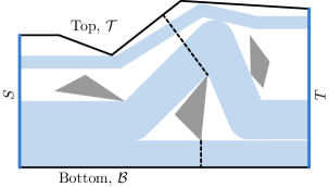
Figure 2: Flow setup. An $S$-$T$ flow decomposed into 3 thick paths (yellow); two edges of the critical graph, defining a cut (dashed).

Let $P$ be a polygonal domain with $n$ vertices, and let the source $S$ and the sink $T$ be two given edges on the outer boundary of $P$ (Fig. 2). A flow in $P$ is a vector field $F:{P}\to\mathbb{R}^{2}$ with the following properties: $\mathrm{div}\,F(p)=0\,\,\forall p\in{P}$ (there are no source/sinks inside the domain), $F(p)\cdot{\bf n}(p)=0\,\,\forall p\in\partial{P}\setminus\{S\cup T\}$ where ${\bf n}(p)$ is the unit normal to the boundary of $P$ at point $p$ (the flow enters/exits $P$ only through the source/sink), and $|F(p)|\leq 1\,\forall p\in{P}$ (the permeability of any point is 1, i.e., not more than a unit of flow can be pushed through any point – the flow respects the capacity constraint). Similarly to the discrete network flow, the value of a continuous flow $F$ is the total flow coming in from the source ($\int_{S}\,F\!\cdot\!{\bf n}\,\,\mathrm{d}s$) – since in the interior of $P$ the flow is divergence-free (flow conserves inside $P$), by the divergence theorem, the value is equal to the total flow out of the sink ($-\int_{T}\,F\!\cdot\!{\bf n}\,\,\mathrm{d}t$). A cut is a partition of $P$ into 2 parts with $S,T$ in different parts (analogous to a cut in a network); the capacity of the cut is the length of the boundary between the parts. Finally, the source and the sink split the outer boundary of $P$ into two parts called the bottom $\mathcal{B}$ and the top $\mathcal{T}$, and the critical graph of the domain [11] is the complete graph on the domain’s holes, $\mathcal{B}$ and $\mathcal{T}$, whose edge lengths equal to the distances between their endpoints (we assume that the edges are embedded to connect the closest points on the corresponding holes, $\mathcal{B}$ or $\mathcal{T}$). The celebrated Flow Decomposition and MaxFlow/MinCut theorems for network flows have continuous counterparts: (the support of) a flow decomposes into (thick) paths [22], and the maximum value of the $S$-$T$ flow is equal to the capacity of the minimum cut [29]; moreover, the mincut is defined by the shortest $\mathcal{B}$-$\mathcal{T}$ path in the critical graph [20].

For shortest path blocking, the setup is a bit more elaborated. Let $s$ be a point on the outer boundary of $P$, and let $S^{*}$ be the edge containing $s$. We assume that $s$ is actually an infinitesimally small gap $s^{-}s^{+}$ in the boundary of $P$ (with $s^{-}$ below $s$ and $s^{+}$ above), and that the union of the barriers and the holes is not allowed to contain a path that starts on $S^{*}$ below $s^{-}$ and ends on $S^{*}$ above $s^{+}$, completely cutting out $s$ (Fig. 3). W.l.o.g. we treat $s^{-}$ and $s^{+}$ as vertices of $P$. Similarly, we are given a point $t$, modeled as a gap $t^{+}t^{-}$ in another edge $T^{*}$ on the outer boundary of $P$.

Figure 3: Path setup; barriers are red and $s$-$t$ path is blue. Surrounding $s^{-}s^{+}$ (left) is forbidden, even if no barrier touches the gap. Completely “shutting the door” $s^{-}s^{+}$ with one barrier (right (a)) is not allowed: if a barrier is at $s$, it must touch at most one of $s^{-},s^{+}$ (right (b,c)).

Let $\mathsf{SP}(p,q)$ denote a shortest path (a geodesic) between points $p$ and $q$ in $P$. Where it creates no confusion, we will identify a path with its length; in particular, for two points $p,q$, we will use $pq$ to denote both the segment $pq$ and its length. The shortest path map from $s$, denoted $\mathsf{SPM}({s})$, is the decomposition of $P$ into cells such that shortest paths $\mathsf{SP}({s},{{p}})$ from $s$ to all points $p$ within a cell visit the same sequence of vertices of $P$; the last vertex in this sequence is called the root of the cell and is denoted by $\mathsf{r}_{{s}}({{p}})$. The shortest path map from $t$ ($\mathsf{SPM}({t})$) and the roots of its cells ($\mathsf{r}_{{t}}({p})$) are defined analogously. The maps have linear complexity and can be built in $O(n\log n)$ time (in $O(n)$ time if $P$ is simple) [21]. Our algorithm for path blocking in a simple polygon uses:

Lemma 1.

[26, Lemma 1] Let $p$, $q$, and $r$ be three points in a simple polygon $P$. The geodesic distance from $p$ to a point $x\in\mathsf{SP}(q,r)$ is a convex function of $x$.

Finally, let $E(u,v,p)$ denote the ellipse with foci $u$ and $v$, going through the point $p$. It is well known that the sum of distances to the foci is constant along the ellipse; for the points outside (resp. inside) the ellipse, the sum is larger (resp. smaller) than $up+pv$. It is also well known that the tangent to the ellipse at $p$ is perpendicular to the bisector of the angle $upv$ (the light from $u$ reaches $v$ after reflecting from the ellipse at $p$).

3 Linear-time algorithms for simple polygons

In this section $P$ is a simple polygon. For a set $X\subset P$, let $\mathsf{SP}_{X}(p,q)$ denote the shortest path between points $p,q$ in ${P}\setminus X$ (and the length of the path), i.e., the shortest $p\textrm{-}q$ path avoiding $X$. We first consider finding the most vital unit barrier for the shortest path, i.e., finding the unit segment $ab$ maximizing $\mathsf{SP}_{ab}({s},{t})$. For the path blocking, we (re)define the bottom $\mathcal{B}$ and top $\mathcal{T}$ of $P$ as the $t^{-}\textrm{-}s^{-}$ and $s^{+}\textrm{-}t^{+}$ parts of $\partial{P}$ resp. (which mimics the flow setup, replacing the entrance $S$ and exit $T$ with $s^{-}s^{+}$ and $t^{-}t^{+}$). We will treat $s^{-},s^{+},t^{-}$, and $t^{+}$ as vertices of $P$. We then prove that a most vital barrier is placed at a vertex of $P$ (Section 3.1). We focus on placing the barrier at (a vertex of) $\mathcal{B}$; placing at $\mathcal{T}$ is symmetric. In Section 3.2 we test whether it is possible for any unit barrier $ab$ touching $\mathcal{B}$ to also touch $\mathcal{T}$ (while not lying on $S^{*}$ or $T^{*}$): if this is possible, the barrier separates $s$ from $t$ completely and $\mathsf{SP}_{ab}(s,t)=\infty$. We test this by computing the Minkowski sum of $\mathcal{B}$ with a unit disk and intersecting the resulting shape with $\mathcal{T}$, taking special care around $s$ and $t$ (to disallow having $ab\subset S^{*}$). In Section 3.3 we then proceed to our main technical contribution: showing how to optimally place a barrier touching (a vertex of) $\mathcal{B}$ given that no such barrier can simultaneously touch $\mathcal{T}$. For this, we compute the shortest $s$-$t$ path $H$ around the Minkowski sum of $\mathcal{B}$ with the unit disk and argue that an optimal barrier will have one endpoint on (a vertex of) $\mathcal{B}$ and the other endpoint on $H$. Furthermore, we show that this path $H$ intersects edges of the shortest path maps $\mathsf{SPM}({s})$ and $\mathsf{SPM}({t})$ only linearly many times. We subdivide $H$ at these intersection points, and show that for each edge $e$ of $H$ we can then calculate the optimal placement of a point on $e$ maximizing the sum of distances to $s$ and $t$. This gives us a linear-time algorithm for finding a single most vital barrier. In Section 3.4 we then show that even if we have multiple barriers, it is best to glue the barriers together into a single super-barrier.

3.1 A most vital barrier is “rooted” at a vertex of $P$

We first make some observations about potentially optimal placements.

Lemma 2.

A most vital barrier touches $\partial{P}$.

Proof.

Suppose that a most vital barrier $ab$ does not touch $\partial{P}$. Clearly, there must be two (equal-length) shortest $s$-$t$ paths, $\pi_{a}$ and $\pi_{b}$, going through $a$ and $b$ resp., for otherwise the shortest path length can be increased by shifting $ab$ along its supporting line. We argue that there is always a direction in which $ab$ can be translated so that the lengths of both $\pi_{a}$ and $\pi_{b}$ increase.

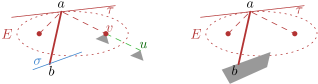
Figure 4: Red dots are $\mathsf{r}_{{s}}({a})$ and $\mathsf{r}_{{t}}({a})$. Left: It is always possible to translate $ab$ so that $a$ moves into $\tau^{+}$ and $b$ moves into $\sigma^{+}$. The tangent will not change when $\mathsf{r}_{{t}}({a})$ jumps from $v$ to $u$. Right: Sliding $b$ to the right lengthens $\pi_{a}$

Consider the ellipse $E=E(\mathsf{r}_{{s}}({a}),\mathsf{r}_{{t}}({a}),a)$ through $a$; let $\tau$ be the tangent to $E$ at $a$, and let $\tau^{+}$ be the (closed) halfplane that does not contain $E$ (Fig. 4, left). In order to increase $\mathsf{r}_{{s}}({a})a+a\mathsf{r}_{{t}}({a})$, the barrier should be moved so that $a$ moves into $\tau^{+}$. Similarly, let $\sigma^{+}$ be the closed halfplane, moving $b$ into which increases $\mathsf{r}_{{s}}({b})b+b\mathsf{r}_{{t}}({b})$ (the halfplane is defined by the tangent $\sigma$, at $b$, to the ellipse $E(\mathsf{r}_{{s}}({b}),\mathsf{r}_{{t}}({b}),b)$). There is a direction $\theta$ so that the rays in direction $\theta$ starting in $a$ and $b$, respectively, are contained in the corresponding half-planes. Hence, we can translate $ab$ in this direction so that both $\mathsf{r}_{{s}}({a})a+a\mathsf{r}_{{t}}({a})$ and $\mathsf{r}_{{s}}({b})b+b\mathsf{r}_{{t}}({b})$ increase. Thus, if none of the roots $\mathsf{r}_{{s}}({a})$, $\mathsf{r}_{{t}}({a})$, $\mathsf{r}_{{s}}({b})$, $\mathsf{r}_{{t}}({b})$ changes as the barrier is translated, the length of both $\pi_{a}$ and $\pi_{b}$ increases.

It remains to deal with the case in which one of the four roots would change during the infinitesimal translation (say, $\mathsf{r}_{{t}}({a})$ changes from a vertex $v$ to a vertex $u$) – i.e., when $a$ belongs to the line $uv$. Let $\tau_{v},\tau_{u}$ be the tangents at $a$ to $E(\mathsf{r}_{{s}}({a}),v,a),E(\mathsf{r}_{{s}}({a}),u,a)$ resp. (refer to Fig. 4, left). Can it be the case that the directions inside $\tau_{v}^{+},\tau_{u}^{+}$ and $\sigma^{+}$ do not have a common direction, i.e., that the good translations defined by $\tau_{u}$ (the ones increasing $\mathsf{r}_{{s}}({a})a+au$) are incompatible with those defined by $\tau_{v}$ (so that $ab$ would be stuck with $a$ on the line $uv$ because the path length would increase both when moving from the cell of $v$ into the cell of $u$ and vice versa)? The answer is no, because $\tau_{v}=\tau_{u}$: the former is perpendicular to the bisector of the angle $\mathsf{r}_{{s}}({a})av$ and the latter is perpendicular to the bisector of the angle $\mathsf{r}_{{s}}({a})au$ – which are the same angle.∎

Lemma 3.

A vertex of a most vital barrier touches $\partial{P}$.

Proof.

Suppose that none of $a,b$ touches the boundary (so $ab$ touches $\partial{P}$ with a point interior to the barrier). Clearly, the shortest $s$-$t$ path, $\pi_{ab}$, must go through both $a$ and $b$, for otherwise the shortest path can be lengthened by moving the barrier; also, $\pi_{ab}$ must make same-direction turns (cw or ccw) at both $a$ and $b$, for otherwise the shortest $s$-$t$ path may bypass the barrier altogether (Fig. 5, left and middle). We claim that it is always possible to move $ab$ along its supporting line (i.e., keeping the contact with $\partial{P}$) increasing the length of $\pi_{ab}$. Indeed, if one of the angles $\mathsf{r}_{{s}}({a})ab,ab\mathsf{r}_{{t}}({b})$ is obtuse and the other is acute (Fig. 5, right), then moving in the direction of the acute angle increases both $\mathsf{r}_{{s}}({a})a$ and $\mathsf{r}_{{t}}({b})b$ (we assume that the path visits $a$ before $b$). If both angles are acute, then, as can be easily seen by differentiation, the derivative of the path length w.r.t. the shift of $ab$ along its supporting line is $\cos(\mathsf{r}_{{s}}({a})ab))-\cos(ab\mathsf{r}_{{t}}({b}))\neq 0$ unless the angles are equal; however, if the angles are equal, the length is at the minimum (which, again, can be seen by differentiation). The case of both angles being obtuse is similar.∎

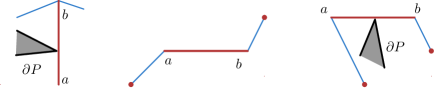
Figure 5: The path is blue, red dots are $\mathsf{r}_{{s}}({a})$ and $\mathsf{r}_{{t}}({b})$. Left: If the path bends only on $b$, moving $ab$ up lengthens $\pi_{b}$. Middle: If the turns are different, $\pi_{ab}$ is not pulled taut. Right: Moving $ab$ left lengthens $\pi_{ab}$

Lemma 4.

There exists a most vital barrier $ab$ in which one endpoint, say $b$, lies on a vertex of $P$.

Proof.

Suppose that the barrier touches the interior of an edge of $P$ (Fig. 4, right). Then the shortest $s$-$t$ path $\pi_{a}$ through $a$ may be lengthened by translating the barrier parallel to itself while sliding $b$ along the edge—the argument is analogous to the one in the proof of Lemma 2: one of the two possible translation directions moves $a$ inside the halfplane $\tau^{+}$. ∎

3.2 Blocking the path from $s$ to $t$ completely

We now argue that we can check in linear time whether it is possible to completely block passage from $s$ to $t$, by placing a barrier that connects $\mathcal{B}$ to $\mathcal{T}$ (without placing the barrier along $S^{*}$ or $T^{*}$, which is forbidden by our model; see Section 2).

Observation 5.

Let $u$ and $v$ be two vertices of $\mathsf{SP}(s,t)$ in $\mathcal{B}$. The geodesic makes a right turn at $u$ if and only if it makes a right turn at $v$. Let $u^{\prime}$ and $v^{\prime}$ be two vertices of $\mathsf{SP}(s,t)$ in $\mathcal{T}$. The geodesic makes a left turn at $u^{\prime}$ if and only if it makes a left turn at $v^{\prime}$. Moreover, if $\mathsf{SP}(s,t)$ makes a right turn in $u$ then it makes a left turn in $u^{\prime}$.

Assume without loss of generality that $\mathsf{SP}(s,t)$ makes a right turn at a vertex $u\in{\mathcal{B}}$. By Observation 5 it thus makes right turns at all vertices of $\mathsf{SP}(s,t)\cap{\mathcal{B}}$, and left turns at all vertices of $\mathsf{SP}(s,t)\cap{\mathcal{T}}$.

Observation 6.

If $\mathsf{SP}(s,t)$ makes a right turn at $u\in{\mathcal{B}}$, and we place a barrier $ur$ at $u$, then $\mathsf{SP}_{ur}(s,t)$ makes a right turn at $r$.

For every point $p$ on $\mathcal{B}$, consider placing a barrier $pq$ of length at most one, with one endpoint on $p$. The possible placements $D_{p}$ of the other endpoint, $q$, form a subset of the unit disk centered at $p$. Let $\mathcal{D}=\bigcup_{p\in{\mathcal{B}}}D_{p}$ denote the union of all these regions (see Fig. 6).

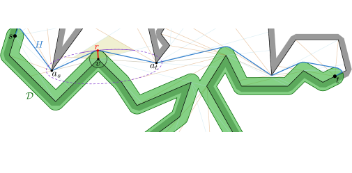
Figure 6: Our algorithm constructs the region $\mathcal{D}$ describing possible placements of a barrier incident to $\mathcal{B}$, and the shortest path $H$ around $\mathcal{D}$. An optimal barrier incident to $\mathcal{B}$ has one endpoint on $H$.

Observation 7.

There is a barrier that separates $s$ from $t$ if and only if $s$ and $t$ are in different components of $P\setminus\mathcal{D}$.

We now observe that $\mathcal{D}$ is essentially the Minkowski sum of $\mathcal{B}$ with a unit disk $D$. More specifically, let $A\oplus B=\{a+b\mid a\in A\land b\in B\}$ denote the Minkowski sum of $A$ and $B$, let $S^{*}_{\mathcal{B}}=S^{*}\cap{\mathcal{B}}$ denote the part of $S^{*}$ in $\mathcal{B}$, let $S^{*}_{\mathcal{T}}$, $T^{*}_{\mathcal{B}}$, and $T^{*}_{\mathcal{T}}$ be defined analogously, and let ${\mathcal{B}}^{\prime}={\mathcal{B}}\setminus(S^{*}_{\mathcal{B}}\cup T^{*}_{\mathcal{B}})$.

Lemma 8.

We have that $\mathcal{D}=\mathcal{D}^{\prime}\cup X_{S}\cup X_{T}$, where $\mathcal{D}^{\prime}={\mathcal{B}}^{\prime}\oplus D$, $X_{A}=(A^{*}_{\mathcal{B}}\oplus D)\setminus A^{*}_{\mathcal{T}}$, and $D$ is the unit disk centered at the origin. Moreover, $\mathcal{D}$ can be computed in $O(n)$ time.

Proof.

The equality follows directly from the definition of $\mathcal{D}$ and the Minkowski sum. It then also follows $\mathcal{D}$ has linear complexity. So we focus on computing $\mathcal{D}$. To this end we separately compute $\mathcal{D}^{\prime}$, $X_{S}$, and $X_{T}$, and take their union. More specifically, we construct the Voronoi diagram of ${\mathcal{B}}^{\prime}$ using the algorithm of Chin, Snoeyink, and Wang [7], and use it to compute ${\mathcal{B}}^{\prime}\oplus D$ [15]. Both of these steps can be done in linear time. Since $S^{*}$, $T^{*}$, and $D$ have constant complexity, we can compute $X_{S}$ and $X_{T}$ in constant time. The resulting sets still have constant complexity, so unioning them with ${\mathcal{B}}^{\prime}\oplus D$ takes linear time. ∎

Lemma 9.

We can test if $s$ and $t$ lie in the same component $C$ of $P\setminus\mathcal{D}$, and compute $C$ if it exists, in $O(n)$ time.

Proof.

Using Lemma 8 we compute $\mathcal{D}$ in linear time. If $s$ or $t$ lies inside $\mathcal{D}$, which we can test in linear time, then $C$ does not exist. Otherwise, by definition of $X_{S}$ and $X_{T}$, $s$ and $t$ must lie on the boundary of $\mathcal{D}$. We then extract the curve $\sigma$ connecting ${s}$ to ${t}$ along the boundary of $\mathcal{D}$, and test if $\sigma$ intersects the top of the polygon $\mathcal{T}$. If (and only if) $\sigma$ and $\mathcal{T}$ do not intersect, their concatenation delineates a single component $C^{\prime}$ of $P\setminus\mathcal{D}$. Since $C^{\prime}$ contains both $s$ and $t$ we have $C=C^{\prime}$. So, all that is left is to test if $\sigma$ and $\mathcal{T}$ intersect. This can be done in linear time by explicitly constructing $C^{\prime}$ and testing if it is simple [6]. ∎

Theorem 10.

Given a simple polygon $P$ with $n$ vertices and two points $s$ and $t$ on the boundary of $P$, we can test whether there exists a placement of a unit length barrier that disconnects $s$ from $t$ in $O(n)$ time.

3.3 Maximizing the length from $s$ to $t$ with a single barrier

In the remainder of the section we assume that we cannot place a barrier on (a vertex of) $\mathcal{B}$ that completely separates $s$ from $t$. Fix a distance $d$, and consider all points $p\in P$ such that $\mathsf{SP}(s,p)+\mathsf{SP}(p,t)=d$. Let $C_{d}$ denote this set of points, and define $C_{\leq d}=\bigcup_{d^{\prime}\leq d}C_{d^{\prime}}$.

Observe that an optimal barrier will have one of its endpoints on the boundary of $\mathcal{D}$. Let $H=\mathsf{SP}_{\mathcal{D}}(s,t)$ be the shortest path from $s$ to $t$ avoiding $\mathcal{D}$. We will actually show that there is an optimal barrier $V^{*}$ whose endpoint $a$ lies on $H$, and that $H$ has low complexity. This then gives us an efficient algorithm to compute an optimal barrier. To show that $a$ lies on $H$ we use that if $V^{*}$ realizes detour $d^{*}$ (i.e., $\mathsf{SP}_{V^{*}}(s,t)=d^{*}$), the endpoint $a$ also lies on $C_{d^{*}}$. First, we prove some properties of $C_{d^{*}}$ towards this end.

Observation 11.

Let $\Delta_{s}$ be a cell in $\mathsf{SPM}(s)$ with root $a_{s}$, and $\Delta_{t}$ be a cell in $\mathsf{SPM}(t)$ with root $a_{t}$. We have that $C_{d}\cap\Delta_{s}\cap\Delta_{t}$ consists of a constant number of intervals along the boundary of the ellipse with foci $a_{s}$ and $a_{t}$.

Proof.

A point $p\in C_{d}$ satisfies $\mathsf{SP}(s,p)+\mathsf{SP}(p,t)=d$. For $p\in\Delta_{s}\cap\Delta_{t}$ we thus have $\mathsf{SP}(s,a_{s})+\|a_{s}p\|+\|pa_{t}\|+\mathsf{SP}(a_{t},t)=d$. Since $d$, $\mathsf{SP}(s,a_{s})$, and $\mathsf{SP}(a_{t},t)$ are constant, this equation describes an ellipse with foci $a_{s}$ and $a_{t}$. Since $\Delta_{s}$ and $\Delta_{t}$ have constant complexity the lemma follows. ∎

Lemma 12.

$C_{\leq d}$ is a geodesically convex set (it contains shortest paths between its points).

Proof.

Let $p$ and $q$ be two points on $C_{d}$, and assume, by contradiction, that there is a point $r$ on $\mathsf{SP}(p,q)$ outside of $C_{\leq d}$. By Lemma 1 the geodesic distance from $s$ to $\mathsf{SP}(p,q)$ is a convex function. Similarly, the distance from $t$ to $\mathsf{SP}(p,q)$ is convex. It then follows that the function $f(x)=\mathsf{SP}(s,x)+\mathsf{SP}(x,t)$, for $x$ on $\mathsf{SP}(p,q)$ is also convex, and thus has its local maxima at $p$ and/or $q$. Contradiction. ∎

Lemma 13.

If there is an optimal barrier $ua$ incident to a vertex $u$ of $\mathcal{B}$, then the ray $\rho$ from $u$ through $a$ intersects $H$.

Proof.

The ray $\rho$ splits $P$ into two subpolygons $P_{1}$ and $P_{2}$. Since $\mathsf{SP}_{ua}(s,t)$ makes a right bend at $a$ (Observation 6 and our assumption that $\mathsf{SP}(s,t)$ makes a right turn at $u$) it intersects both subpolygons $P_{1}$ and $P_{2}$. It is easy to show that therefore $s$ and $t$ must be in different subpolygons (otherwise the geodesic crosses $\rho$ a second time, and we could shortcut the path along $\rho$). Since $H$ connects $s$ to $t$ it must thus also intersect $\rho$. ∎

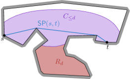
Figure 7: A sketch of the regions $C_{\leq d}$ (purple) and $R_{d}$. Observe that $R_{d}$ cannot contain any vertices of ${\mathcal{T}}$, otherwise ${\mathcal{T}}$ would have to pierce $\mathsf{SP}(s,t)$ and thus $C_{\leq d}$.

Next, we define the region $R_{d}$ “below” $C_{\leq d}$. More formally, let $R^{\prime}$ be the region enclosed by ${\mathcal{B}}$ and $\mathsf{SP}(s,t)$, let $d\geq\mathsf{SP}(s,t)$, and let $R_{d}=R^{\prime}\setminus C_{\leq d}$. See Fig. 7. We then argue that it is separated from the top part of our polygon $\mathcal{T}$, which allows us to prove that there is an optimal barrier with an endpoint on $H$.

Observation 14.

Region $R_{d}$ contains no vertices of $\mathcal{T}$.

Proof.

Assume, by contradiction that there is a vertex of $\mathcal{T}$ in $R_{d}$. Observe that this disconnects $C_{\leq d}$. However, since $C_{\leq d}$ is geodesically convex (Lemma 12) and non-empty it is a connected set. Contradiction. ∎

Lemma 15.

If there is an optimal barrier $ua$ where $u$ is a vertex of $\mathcal{B}$, then there is an optimal barrier $ur$ where $r$ is a point on $D_{u}\cap H$ (recall that $D_{u}$ is the unit disk centered at $u$).

Proof.

Assume, by contradiction, that there is no optimal barrier incident to $u$ that has its other endpoint on $H$. Consider the ray from $u$ in the direction of $a$. By Lemma 13, the ray hits $H$ in a point $r^{\prime}$ (Fig. 8). Because $a$ lies on $C_{d^{*}}$ and $C_{\leq d^{*}}$ is geodesically convex (Lemma 12), $r^{\prime}$ lies outside $C_{\leq d^{*}}$. Let $H[p,q]=\mathsf{SP}_{\mathcal{D}}(p,q)$ be the maximal (open ended) subpath of $H$ that contains $r^{\prime}$ and lies outside of $C_{\leq d^{*}}$. We then distinguish two cases, depending on whether or not $H[p,q]$ intersects (touches) $\mathcal{D}$:

Figure 8: Illustration of Lemma 15.

$H{[p,q]}$ does not intersect (touch) $\mathcal{D}$.

It follows that $H[p,q]$ is a geodesic in $P$ as well, i.e. $H[p,q]=\mathsf{SP}(p,q)$. Since $p,q\in C_{\leq d^{*}}$, and $C_{\leq d^{*}}$ is geodesically convex (Lemma 12) we then have that $H[p,q]\subseteq C_{\leq d^{*}}$. Contradiction.

$H{[p,q]}$ intersects $\mathcal{D}$ in a point $z$.

Let $v\in B$ be a point such that $z\in D_{v}$. We distinguish two subcases, depending on whether $z$ lies in the region $R_{d^{*}}$.

$z\in R_{d^{*}}$.

In this case $z$ lies “below” $C_{\leq d^{*}}$. From $z\in H$ it follows that $H[p,q]\subset R_{d^{*}}$. However, as $C_{d^{*}}$ is geodesically convex, this must mean that $H[p,q]$ has a vertex $w$ in $R_{d^{*}}$ at which it makes a left turn. This implies that $w$ is a vertex of $\mathcal{T}$. By Observation 14 there are no vertices of $\mathcal{T}$ in $R_{d^{*}}$. Contradiction.

$z\not\in R_{d^{*}}$

Observe that $vz$ is a valid candidate barrier. Since $z\not\in C_{\leq d^{*}}$, the point $z$ actually lies above (i.e. to the left of) $\mathsf{SP}(s,t)$, and thus $\mathsf{SP}_{vz}(s,t)$ makes a right turn at $z$. Using that $z\not\in C_{\leq d^{*}}$ it follows that $\mathsf{SP}_{vz}(s,t)>d^{*}$. This contradicts that $d^{*}$ is the maximal detour we can achieve.

Since all cases end in a contradiction this concludes the proof. ∎

We now know there exists an optimal barrier with an endpoint on $H$. Next, we focus on the complexity of $H$.

Observation 16.

Let $b$ and $c$ be two points on $H$, such that $H$ makes a left turn in between $b$ and $c$ (i.e. the subcurve $H[b,c]$ of $H$ between $b$ and $c$ intersects the half-plane right of the supporting line of $bc$). Then $H[b,c]$ contains a vertex of $\mathcal{T}$.

Lemma 17.

The curve $H$ intersects an edge $e$ of $SPM(z)$, with $z\in\{s,t\}$, at most twice. Hence, $H$ intersects $\mathsf{SPM}(z)$ at most $O(n)$ times.

Proof.

If $e$ is a polygon edge, then $H$ cannot intersect $e$ at all, so consider the case when $e$ is interior to $P$. Assume, by contradiction, that $H$ intersects $e$ at least three times, in points $a$, $b$, and $c$, in that order along $H$ (Fig. 9).

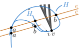
Figure 9: The two cases in the proof of Lemma 17.

If the intersections $a$, $b$, and $c$, are also consecutive along $e$, then $H$ makes both a left and right turn in between $a$ and $c$. It is easy to see that since $H$ can bend to the left only at vertices of ${\mathcal{T}}$ (Observation 16), the region (or one of the two regions) enclosed by $H$ and $ac$ must contain a polygon vertex. Since both $e$ and $H[a,c]$ lie inside $P$, this means that $P$ has a hole. Contradiction.

If the intersections are not consecutive, (say $a,c,b$), then again there is a region enclosed by $H[a,c]$ and $ab$, containing a polygon vertex. Since both $H[b,c]$ and $cb$ lie inside $P$, this vertex must lie on a hole. Contradiction. ∎

Algorithm.

We compute intersections of $H$ with the shortest path maps $\mathsf{SPM}(s)$ and $\mathsf{SPM}(t)$, and subdivide $H$ at each intersection point. By Lemma 17, the resulting curve $H^{\prime}$ still has only linear complexity. Consider the edges of $H^{\prime}$ in which $H^{\prime}$ follows the boundary of $D_{v}$, for the vertices $v$ of $\mathcal{B}$. By Lemma 15 for some $v\in{\mathcal{B}}$ there is an optimal barrier that has one endpoint on such an edge of $H^{\prime}$ and the other at $v$. Since $H^{\prime}$ has only $O(n)$ edges we simply try each edge $e$ of $H^{\prime}$. For all points $r\in e$, the geodesics $\mathsf{SP}(s,r)$ and $\mathsf{SP}(t,r)$ have the same combinatorial structure, i.e., the roots $a_{s}=\mathsf{r}_{{s}}({r}),a_{t}=\mathsf{r}_{{t}}({r})$ stay the same. It follows that we have a constant-size subproblem in which we can compute an optimal barrier in constant time. Specifically, we compute the smallest ellipse $E$ with foci $a_{s}$ and $a_{t}$ that contains $e$ and goes through the point $r$ in which $E$ and $e=D_{v}$ have a common tangent (if such a point exists). See Fig. 6. For that point $r$, we then also know the length of the shortest path $\mathsf{SP}_{vr}(s,t)=\mathsf{SP}(s,r)+\mathsf{SP}(r,t)$, assuming that we place the barrier $vr$. We then report the point $r$ that maximizes this length over all edges of $H^{\prime}$.

Constructing the connected component $P^{\prime}$ of $P\setminus\mathcal{D}$ that contains $s$ and $t$ takes linear time (Lemma 9). This component $P^{\prime}$ is a simple splinegon, in which we can compute the shortest path $H$ connecting $s$ to $t$ in $O(n)$ time [19]. Computing $\mathsf{SPM}(s)$ and $\mathsf{SPM}(t)$ also requires linear time [13]. We can then walk along $H$, keeping track of the cells of $\mathsf{SPM}(s)$ and $\mathsf{SPM}(t)$ containing the current point on $H$. Computing the ellipse, the point $p$ on the current edge $e$, and the length of the geodesic takes constant time. It follows that we can compute an optimal barrier incident to $\mathcal{B}$ in linear time. We use the same procedure to compute an optimal barrier incident to $\mathcal{T}$. We thus obtain the following result.

Theorem 18.

Given a simple polygon $P$ with $n$ vertices and two points $s$ and $t$ on $\partial P$, we can compute a unit length barrier that maximizes the length of the shortest path between $s$ and $t$ in $O(n)$ time.

3.4 Using multiple vital barriers

We prove a structural property that even when we are given many barriers, there always exists an optimal solution in which they glued into a single super-barrier. This implies that our linear-time algorithm from the previous section can still be used to solve the problem.

Clearly, any solution distributes the barriers over some (unknown) number of super-barriers. First observe that, similarly to Section 3.1, any super-barrier must have a vertex at a vertex of $P$, and the next lemmas prove that it is suboptimal to have more than one such super-barrier.

The first lemma is a variant of Lemma 1. Let $a_{1}b_{1}$ and $a_{2}b_{2}$ be two segments inside $P$, and let $m_{1}\in a_{1}b_{1},m_{2}\in a_{2}b_{2}$ be two points that divide the segments in the same proportion, that is $\vec{m_{1}}=\gamma\vec{a_{1}}+(1-\gamma)\vec{b_{1}},\vec{m_{2}}=\gamma\vec{a_{2}}+(1-\gamma)\vec{b_{2}}$ for some $\gamma\in[0,1]$. Define function $f(\gamma)=\mathsf{SP}(m_{1},m_{2})$.

Lemma 19.

$f(\gamma)$ is convex for $\gamma\in[0,1]$: $\mathsf{SP}(m_{1},m_{2})\leq\gamma\mathsf{SP}(a_{1},a_{2})+(1-\gamma)\mathsf{SP}(b_{1},b_{2})\,.$

Proof.

Consider two cases: when the paths $\mathsf{SP}(a_{1},a_{2}),\mathsf{SP}(b_{1},b_{2})$ intersect and when they do not.

Case 1. Paths $\mathsf{SP}(a_{1},a_{2})$ and $\mathsf{SP}(b_{1},b_{2})$ intersect (Fig. 10, left). Choose some intersection point $c$. From Lemma 1 it follows that a shortest path from a fixed point to a point on a given segment is a convex function. Then,

$$\mathsf{SP}(c,m_{1})\leq\gamma\mathsf{SP}(c,a_{1})+(1-\gamma)\mathsf{SP}(c,b_{1})\,\quad\text{ and }\quad\mathsf{SP}(c,m_{2})\leq\gamma\mathsf{SP}(c,a_{2})+(1-\gamma)\mathsf{SP}(c,b_{2})\,.$$

By triangle inequality,

$$\mathsf{SP}(m_{1},m_{2})\leq\mathsf{SP}(c,m_{1})+\mathsf{SP}(c,m_{2})\,.$$

Thus,

$$\mathsf{SP}(m_{1},m_{2})\leq\gamma\mathsf{SP}(a_{1},a_{2})+(1-\gamma)\mathsf{SP}(b_{1},b_{2})\,.$$

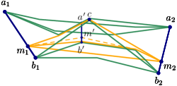
Figure 10: From left to right: Cases 1, 2a, 2b from Lemma 19.

Case 2. Paths $\mathsf{SP}(a_{1},a_{2})$ and $\mathsf{SP}(b_{1},b_{2})$ do not intersect.

Case 2a. Suppose the path $\mathsf{SP}(m_{1},m_{2})$ is also disjoint from the paths $\mathsf{SP}(a_{1},a_{2})$ and $\mathsf{SP}(b_{1},b_{2})$ (Fig. 10, middle). Because $P$ is a simple polygon, the path $\mathsf{SP}(m_{1},m_{2})$ must be a straight-line segment. By simple vector manipulation we can show that $m_{1}m_{2}\leq\gamma a_{1}a_{2}+(1-\gamma)b_{1}b_{2}$, and thus,

$$\mathsf{SP}(m_{1},m_{2})=m_{1}m_{2}\leq\gamma a_{1}a_{2}+(1-\gamma)b_{1}b_{2}\leq\gamma\mathsf{SP}(a_{1},a_{2})+(1-\gamma)\mathsf{SP}(b_{1},b_{2})\,.$$

Case 2b. Finally, w.l.o.g., assume that the path $\mathsf{SP}(m_{1},m_{2})$ intersects $\mathsf{SP}(b_{1},b_{2})$, but not $\mathsf{SP}(a_{1},a_{2})$ (Fig. 10, right). Let vertex $b^{\prime}$ of $P$ lie on both paths $\mathsf{SP}(m_{1},m_{2})$ and $\mathsf{SP}(b_{1},b_{2})$. Because $P$ is a simple polygon, there exists a point $a^{\prime}\in\mathsf{SP}(a_{1},a_{2})$ visible to $b^{\prime}$. Let $m^{\prime}\in a^{\prime}b^{\prime}$ divide the segment $a^{\prime}b^{\prime}$ in the same proportion, i.e., $\vec{m^{\prime}}=\gamma\vec{a^{\prime}}+(1-\gamma)\vec{b^{\prime}}$. We can apply the same line of reasoning to the segments $a_{1}b_{1}$ and $a^{\prime}b^{\prime}$, and the segments $a^{\prime}b^{\prime}$ and $a_{2}b_{2}$. Either the case 2a will hold, or we have arrived at the same case 2b but a smaller size instance. Thus, recursively we can show that

$$\mathsf{SP}(m_{1},m^{\prime})\leq\gamma\mathsf{SP}(a_{1},a^{\prime})+(1-\gamma)\mathsf{SP}(b_{1},b^{\prime})\,,$$

and

$$\mathsf{SP}(m^{\prime},m_{2})\leq\gamma\mathsf{SP}(a^{\prime},a_{2})+(1-\gamma)\mathsf{SP}(b^{\prime},b_{2})\,.$$

By the triangle inequality we have that $\mathsf{SP}(m_{1},m_{2})\leq\mathsf{SP}(m_{1},m^{\prime})+\mathsf{SP}(m^{\prime},m_{2})$, and thus

$$\mathsf{SP}(m_{1},m_{2})\leq\gamma\mathsf{SP}(a_{1},a_{2})+(1-\gamma)\mathsf{SP}(b_{1},b_{2})\,.\qed$$

Lemma 20.

Given two barriers, possibly of different lengths, an optimal configuration will stack them into a single super-barrier.

Proof.

First note that if the two barriers intersect, their endpoints must coincide. To see this, treat one of the barriers as (a part of) a hole; then, by Lemmas 25 and 26 (which are proved in Section 5 analogously to Lemmas 2 and 3) and Lemma 4, the barriers must touch each other with their vertices. It is easy to see that at the point of the touching, the barriers must form a $180^{\circ}$ angle. In what follows we will assume that the barriers are disjoint.

Let the two barriers be the segments $pm_{1},qm_{2}$ where $p,q$ are vertices of $P$, and let $\alpha,\beta$ be their lengths. Let point $a$ lie on the extension of segment $pm_{1}$ into $P$ with $m_{1}a=qm_{2}=\beta$ (i.e., extend $pm_{1}$ for distance $\beta$); similarly, let $b$ lie on the extension of $qm_{2}$ with $m_{2}b=pm_{1}=\alpha$ (Fig. 11). If $m_{1}a$ (or $m_{2}b$) intersects the polygon boundary, then either $s$ and $t$ get disconnected, or the shortest path from $s$ to $t$ cannot pass through $m_{1}$ (or $m_{2}$ resp.). In both cases, the original configuration of the barriers was not optimal.

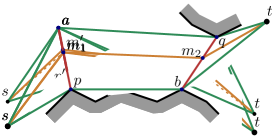
Figure 11: Illustration to Lemma 20. The potential barriers are red.

Then, assume that $m_{1}a$ and $m_{2}b$ are interior to $P$. W.l.o.g. assume that $m_{1}$ lies between $s$ and $m_{2}$ on the shortest path from $s$ to $t$. For simplicity assume that the path $\mathsf{SP}(s,b)$ passes through point $p$, and that the path $\mathsf{SP}(a,t)$ passes through point $q$ (Fig. 11, left and middle). Later we will lift this assumption.

Applying Lemma 1 we get that

$$\mathsf{SP}(s,m_{1})\leq\frac{\alpha}{\alpha+\beta}\mathsf{SP}(s,a)+\frac{\beta}{\alpha+\beta}\mathsf{SP}(s,p)\,,$$

and

$$\mathsf{SP}(m_{2},t)\leq\frac{\beta}{\alpha+\beta}\mathsf{SP}(b,t)+\frac{\alpha}{\alpha+\beta}\mathsf{SP}(q,t)\,.$$

Applying Lemma 19 we get that

$$\mathsf{SP}(m_{1},m_{2})\leq\frac{\alpha}{\alpha+\beta}\mathsf{SP}(a,q)+\frac{\beta}{\alpha+\beta}\mathsf{SP}(p,b)\,.$$

Then, summing up these inequalities we get

$$\mathsf{SP}_{pm_{1},qm_{2}}(s,t)=\mathsf{SP}(s,m_{1})+\mathsf{SP}(m_{1},m_{2})+\mathsf{SP}(m_{2},t)\\ \leq\frac{\alpha}{\alpha+\beta}(\mathsf{SP}(s,a)+\mathsf{SP}(a,q)+\mathsf{SP}(q,t))+\frac{\beta}{\alpha+\beta}(\mathsf{SP}(s,p)+\mathsf{SP}(p,b)+\mathsf{SP}(b,t))\\ =\frac{\alpha}{\alpha+\beta}\mathsf{SP}_{pa}(s,t)+\frac{\beta}{\alpha+\beta}\mathsf{SP}_{pb}(s,t)\,.$$

Thus, either $\mathsf{SP}_{pm_{1},qm_{2}}(s,t)\leq\mathsf{SP}_{pa}(s,t)$ or $\mathsf{SP}_{pm_{1},qm_{2}}(s,t)\leq\mathsf{SP}_{pb}(s,t)$ (or both).

Now assume that path $\mathsf{SP}(s,b)$ intersects segment $pa$ in point $p^{\prime}$, and path $\mathsf{SP}(a,t)$ intersects $qb$ in point $q^{\prime}$ (Fig. 11, right). Then, let points $m^{\prime}_{1}$ and $m^{\prime}_{2}$ be the points dividing the segments $p^{\prime}a$ and $q^{\prime}b$ in the proportion $\alpha:\beta$ and $\beta:\alpha$ respectively. Applying the same argument as above, we get that

$$\mathsf{SP}_{pm_{1},qm_{2}}(s,t)\leq\frac{\alpha}{\alpha+\beta}\mathsf{SP}_{pa}(s,t)+\frac{\beta}{\alpha+\beta}\mathsf{SP}_{pb}(s,t)\,.$$

It also must hold that

$$\mathsf{SP}_{pm^{\prime}_{1},qm^{\prime}_{2}}(s,t)\geq\mathsf{SP}_{pm_{1},qm_{2}}(s,t)\,.$$

We can again conclude that at least one of the following inequalities hold, $\mathsf{SP}_{pm_{1},qm_{2}}(s,t)\leq\mathsf{SP}_{pa}(s,t)$ or $\mathsf{SP}_{pm_{1},qm_{2}}(s,t)\leq\mathsf{SP}_{pb}(s,t)$. That is, the original configuration of the two blocking barriers is not optimal. ∎

Lemma 20 resolves the question for two barriers that are attached to the boundary of ${P}$. We use induction to extend the result to an arbitrary number of barriers.

Theorem 21.

Given a simple polygon $P$ with $n$ vertices, two points $s$ and $t$ on $\partial P$, and $k$ unit-length barriers, the optimal placement of the barriers which maximizes the length of the shortest path between $s$ and $t$ consists of a single super-barrier.

Proof.

We use induction on $k$. The base case for $k=2$ follows from Lemma 20.

First, we argue that Lemma 2 generalizes to arbitrary rigid configurations of barriers: as we translate the configuration, the length of the shortest path above (below) the configuration is a convex differentiable function in the translation vector, and hence there must still be at least one direction in which the configuration can be translated so as to increase the lengths of both paths. Thus, we may assume that the optimal configuration of the $k$ barriers touches $\partial{P}$.

But now, consider (one of) the barrier that touches $\partial{P}$, and consider it to be part of ${P}$. By the induction hypothesis, the remaining $k-1$ barriers are combined into a single super-barrier. But then, the optimal solution for $k$ barriers must be the same as the optimal solution to a problem in which we have only two barriers: one of length $1$ and one of length $k-1$. We apply Lemma 20 again and conclude that the optimal solution uses, in fact, a single super-barrier of length $k$. ∎

Theorem 21 implies that placing an arbitrary set of barriers reduces to placing just one super-barrier, so our linear-time algorithm from the previous section applies.

3.5 Most vital barriers for the flow

In simple polygons the critical graph has only two vertices – $\mathcal{B}$ and $\mathcal{T}$ (which, for the flow blocking, are the $T\textrm{-}S$ and $S\textrm{-}T$ parts of $\partial{P}$; refer to Fig. 2). Flow blocking thus boils down to finding the shortest $\mathcal{B}$-$\mathcal{T}$ connection (then all the barriers will be placed along the connecting segment) – a problem that was solved in linear time in [20].

4 Hardness results

In the remainder of the paper $P$ is a polygonal domain with holes (as defined in Section 2). We first show that in general it is hard to decide whether full blockage can be achieved, i.e., whether it is possible to decrease the $S$-$T$ flow to 0 or to lengthen the $s$-$t$ path to infinity:

Theorem 22.

Flow-HBD and path-HBD are NP-hard.

Proof.

Figure 12: Full blockage is possible iff each channel is fully blocked

Figure 12 shows the reduction for flow-HBD (for path-HBD, just replace the edges $S,T$ with the points $s$,$t$): given an instance of 3-Partition (“Can $3m$ given integers $\{a_{1}\dots a_{3m}\}$ be split into triples so that the sum of integers in each triple is equal to $B=\sum a_{i}/m$?”), construct the domain with $m$ width-$B$ channels between $S$ and $T$, and have a length-$a_{i}$ barrier (line segment) for each integer $i=1\dots 3m$; the barriers can cut $S$ from $T$ iff the 3-Partition instance is feasible. ∎

With different-length barriers, the full blockage remains (weakly) hard even if $n=O(1)$ (and the number of holes is, of course, also small):

Theorem 23.

Flow-hBD and path-hBD are weakly NP-hard.

Proof.

Given an instance of 2-Partition (“Can $m$ given integers $\{a_{1}\dots a_{m}\}$ be split into two sets so that the sum of integers in set is equal to $B=\sum a_{i}/2$?”), construct the domain with $2$ width-$B$ channels between $S$ and $T$ (analogously to the proof of Theorem 22), and have a length-$a_{i}$ barrier for each integer $i=1\dots m$; the barriers can cut $S$ from $T$ iff the 2-Partition instance is feasible. ∎

If all barriers have the same length, deciding possibility of full blockage is polynomial; in fact, Section 5.1 shows that even the more general flow-HB1 problem (finding how to maximally decrease the flow) can be solved in polynomial time. On the contrary, (partial) path blockage is hard even for unit barriers:

Theorem 24.

Path-HB1 is weakly NP-hard.

Proof.

Given an instance $A=\{a_{1}\dots a_{m}\}$ of 2-Partition, we construct a domain with $O(m)$ vertices, in which it is possible to place $m$ unit barriers so that the shortest $s$-$t$ path has length $C+\sum(A)/2$ (where $C$ is some number and $\sum(X)$ is the sum of numbers in a set $X$), iff $A$ can be partitioned into two sets $R$ and $B$ with $\sum(R)=\sum(B)=\sum(A)/2$.

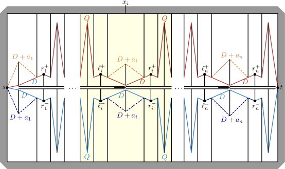
Figure 13: An overview of the construction.

Our construction is sketched in Fig. 13. The main idea is that there are three main routes from $s$ to $t$: a very short middle route, a “red” (top) route, and a “blue” (bottom) route. The red and blue routes both have length $C=mD+(m-1)E$, for some large constants $D$ and $E$, and are much longer than the middle route. We make it such that with exactly $m$ barriers, we can block off the middle route completely. Moreover, by placing a barrier $i$ appropriately, we can increase the length of either the red route or the blue route by exactly $a_{i}$. Increasing the length of the red route by $a_{i}$ corresponds to assigning $a_{i}$ to $R$ and increasing the length of the blue route by $a_{i}$ corresponds to assigning $a_{i}$ to $B$. So, in the end the length of the red and blue routes are $C+\sum(R)$ and $C+\sum(B)$, respectively. Hence, it is possible to partition $A$ into $R$ and $B$, with $\sum(R)=\sum(B)=\sum(A)/2$ if and only if the length of the shortest path between $s$ and $t$ is at least $C+\sum(A)/2$.

Description of the Construction.

In detail, the outer boundary of $P$ is a large rectangle, centered vertically at the $x$-axis and $s$ at the origin.

Our middle route will consist of a rectangular corridor of height $1/2$ vertically centered at the $x$-axis. We cut through the top and bottom walls of the corridor in $m$ intervals $[x_{i}-\varepsilon,x_{i}]$, for some arbitrarily small $\varepsilon>0$. Let $e_{i}$ and $f_{i}$ be the points with $x$-coordinate $x_{i}$ on the top and bottom wall, respectively. See Fig. 14. We build another horizontal segment $h_{i}$ of length $H>2m+\sum(A)$ whose right endpoint is $(x_{i},0)$. Note that we have vertices with exactly the same $x$-coordinate; also note that in order for the construction to work, we must allow placing the barrier so that it contains vertices of the domain.

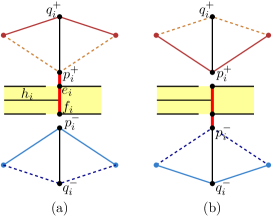
Figure 14: The two possible placements for barrier $i$.

Our red (top) and blue (bottom) routes are completely symmetric, so we describe only the top route. For each opening $[x_{i}-\varepsilon,x_{i}]$ in the middle corridor, we build a vertical segment $p^{+}_{i}q^{+}_{i}$ with bottom endpoint $p^{+}_{i}=(x_{i},3/4)$. In between every consecutive pair $x_{i},x_{i+1}$ we build three long vertical walls attached to the middle corridor, and three long vertical walls attached to the top boundary of $P$ that force the red route to zigzag (see Fig. 13). Let $r^{+}_{i}$, $k_{i}$, and $\ell^{+}_{i+1}$ be the top-endpoints of the walls connected to the middle corridor. The distances between these walls (and the walls extending from the top of $P$) are all large, i.e., larger than $m$, so that we cannot block the passage even if we place all barriers consecutively. The walls extending from the top of $\partial P$ are built so that the length of the shortest path between $r^{+}_{i}$ and $\ell^{+}_{i+1}$ via $k_{i}$, i.e. our zigzag, is very large, say $Q>m^{2}+\sum(A)$. Let $D>2m$ be the distance from $\ell^{+}_{i}$ via $p^{+}_{i}$ to $r^{+}_{i}$. We place $q^{+}_{i}$ (and the endpoints of the walls extending from the top) such that the distance from $\ell^{+}_{i}$ via $q^{+}_{i}$ to $r^{+}_{i}$ is $D+a_{i}$.

Making sure that we use $m$ barriers to block the middle route.

Note that for the shortest $s$-$t$ path to have length at least $C=m(Q+D)>m^{3}+m\sum(A)$, it needs to pass through at least $m$ zigzags from our red or blue routes. Hence, we need to block the middle route between any pair of consecutive openings $x_{i}$ and $x_{i+1}-\varepsilon$. Since we have exactly $m$ barriers, we have to place one barrier, say barrier $i$, to close off the middle corridor between $x_{i}$ and $x_{i+1}$.

Next, observe that if we place barrier $i$ to block off the middle corridor between $x_{i}$ and $x_{i+1}-\varepsilon$ at some $x$-coordinate other than $x_{i}$, we can just shift it to $x_{i}$ without decreasing the length of the shortest path. Furthermore note that connecting the left endpoint of the bottom gap to the right endpoint of the top gap allows either the top or the bottom path to bypass one of the long “spikes” of length $Q$, hence such a placement is non-optimal.

Claim: Any shortest path either stays entirely above middle route or entirely below it.

We now argue that there are only two potential shortest paths left: one that stays entirely above the middle corridor, and one that stays below it. Suppose that a shortest path $\pi$ goes through the $i^{\text{th}}$ zigzag on the red route, i.e., above the corridor, and thus passes through $\ell^{+}_{i}$, and then crosses the middle route to $r^{-}_{i}$. Since we place barrier $i$ at $x_{i}$, this path has to go around the horizontal segment $h_{i}$. It follows that the length of this path is at least $X+2H+Y\geq X+2(m+\sum(A))+Y$, where $X=\mathsf{SP}(s,\ell^{+}_{i})$ and $Y=\mathsf{SP}(r^{-}_{i},t)$ are the shortest ${s}\textrm{-}\ell^{+}_{i}$ and $r^{-}_{i}\textrm{-}t$ paths. Now consider the subpath of $\pi$ from $r^{-}_{i}$ to $t$, and mirror it in the $x$-axis. Observe that this does not increase its length, and that this path $\pi^{\prime}$ now goes through $r^{i}_{+}$. Now consider the path that follows $\pi$ to $\ell^{+}_{i}$, then goes to $r^{+}_{i}$ via $q^{+}_{i}$, and then uses $\pi^{\prime}$ from $r^{+}_{i}$ to $t$. This path has length $X+D+a_{i}+Y$ and is thus shorter than $\pi$. That is, $\pi$ cannot be a shortest path. It follows that any shortest path either stays entirely above or below the middle corridor.

Increasing the length of either the red or blue route by $a_{i}$.

Finally, we argue that if we place barrier $i$ exactly between $f_{i}$ and $p^{+}_{i}$ we can increase the length of the shortest path between $\ell^{+}_{i}$ and $r^{+}_{i}$ by an additional $a_{i}$. Symmetrically, placing barrier $i$ between $e_{i}$ and $p^{-}_{i}$ instead increases the path between $\ell^{-}_{i}$ and $r^{-}_{i}$ by an additional $a_{i}$.

It now follows that the length of the “red” shortest path that stays entirely above the middle corridor and the length of the “blue” shortest path that stays entirely below both have length (at least) $C+\sum(A)/2$ if and only if we can partition $A$ into two subsets $R$ and $B$ with $\sum(R)=\sum(B)=\sum(A)/2$. ∎

Membership in NP for our problems is open, since verifying solutions involve summing square roots.

5 Polynomial-time algorithms

We start from blocking path with one barrier. Recall that two $s$-$t$ paths in the domain have the same homotopy type if they can be continuously (without intersecting the obstacles) morphed to each other. A locally shortest (or “pulled taut”) path is the shortest path within its homotopy type. We consider only those homotopy types for which the locally shortest paths do not self-intersect or self-touch. The shortest $s$-$t$ path $\mathsf{SP}({s},{t})$ is the shortest path of all locally shortest paths. It is well known that shortest paths lie on edges of the visibility graph $VG({P})$ that connects mutually visible vertices of the domain.

When speaking about a path or a path type, we will assume that the path or the path type exists and is locally shortest: that is, a statement like “shortest path of type X” should read “locally shortest path of type X, if such exists” (if a path does not exist, its length is set to infinity). We will also assume that any shortest path $\pi$ that we speak about is unique (again, omitting the modality “if such a path exists”); otherwise, $\pi$ will mean an arbitrary shortest path of the spoken type.

The shortest $s$-$t$ path in the presence of $ab$ is the shorter among the following:

• the shortest path $\pi$ that does not intersect (touch) $ab$ (i.e., the shortest path that goes neither through $a$ nor through $b$)

• the shortest path(s) intersecting $ab$.

The latter type of paths can be of the following subtypes (Fig. 16):

• $\pi_{a}$ going through $a$ but not $b$

• $\pi_{b}$ going through $b$ but not $a$

• $\pi_{a,b}$ going through both $a$ and $b$. This can either be a path $\pi_{\tilde{ab}}$ that uses more than one edge between $a$ and $b$ (if the barrier intersects a hole), or a path $\pi_{ab}$ that has $ab$ as an edge (if $a$ and $b$ are mutually visible).

Figure 15: The paths (dashed) competing to be the shortest: $\pi$ and $\pi_{\tilde{ab}}$ (left), $\pi_{a}$ and $\pi_{b}$ (middle), $\pi_{ab}$ (right); $s$ and $t$ are the dots, and $ab$ is bold red.

Figure 16: Left: $\pi_{a}$ starting/stopping to be pulled taut implies $a$ moving over the edge of $VG({P})$ (dashed); red dots are $\mathsf{r}_{{s}}({a})$ and $\mathsf{r}_{{t}}({b})$. Right: formula for path length changes when and edge of $VG(\bar{P})$ appears/disappears.

The next two lemmas show that the shortest path through the most vital barrier cannot be of the last subtype, i.e., that none of $\pi_{\tilde{ab}},\pi_{ab}$ can be an optimal shortest path:

Lemma 25.

$\pi_{\tilde{ab}}$ cannot be the shortest path for the most vital barrier (segment) $ab$.

Proof.

Analogously to Lemma 2, there is always a direction in which $ab$ can be moved so that the lengths of both $\mathsf{r}_{{s}}({a})a+a\mathsf{r}_{{t}}({a})$ and $\mathsf{r}_{{s}}({b})b+b\mathsf{r}_{{t}}({b})$ increase, lengthening the path.∎

Lemma 26.

$\pi_{ab}$ cannot be the shortest path for the most vital barrier $ab$.

Proof.

Analogous to Lemma 3.∎

Say that two placements of $ab$ are combinatorially equivalent if in both placements each of $a,b$ lies within the same cell of each of $\mathsf{SPM}({s})$ and $\mathsf{SPM}({t})$, and in both placements the barrier intersects the same set of edges of $VG({P})$; say that the equivalence class defines the combinatorial type of the barrier’s placement. For a fixed combinatorial type, it is easy to write lengths of all the competitor paths $\pi,\pi_{a},\pi_{b}$ as functions of $a$ and $b$. Indeed, $\pi$ stays the same, as the same edges of the visibility graph are blocked by $ab$, while $\pi_{a}$ either always stays pulled taut (and hence its length is $\mathsf{SP}({s},{\mathsf{r}_{{s}}({a})})+\mathsf{r}_{{s}}({s})a+a\mathsf{r}_{{t}}({a})+\mathsf{SP}({t},{\mathsf{r}_{{t}}({a})})$) or is never pulled taut (and hence is out of the competition) – this is because when $\pi_{a}$ starts (resp. stops) being pulled taught the visibility edge between $\mathsf{r}_{{s}}({a})$ and $\mathsf{r}_{{t}}({a})$ starts (resp. stops) being cut by $ab$ (Fig. 16, left); similarly for $\pi_{b}$.

We scroll through all combinatorial types of the barrier placement; since $\mathsf{SPM}({s})$ and $\mathsf{SPM}({t})$ have linear complexity and the visibility graph has $O(n^{2})$ edges, the number of combinatorial types is polynomial. For each type, we compute the lower envelope of the lengths of the competing paths (the envelope defines the shortest $s$-$t$ path) and take the highest point on the envelope.

We continue to placing a constant number of barriers.

Theorem 27.

Path-HbD, and hence path-hbD, path-Hb1 and path-hb1, are polynomial.

Proof.

If the number of barriers is constant, only $O(1)$ different sets of super-barriers can be formed, and each such set has $O(1)$ super-barriers (since there were a constant number of barriers to start from). Below we will describe how to deal with one such set; we call the super-barriers in the set just “barriers”.

Similarly to finding one most vital barrier, we say that two placements of the barriers are combinatorially equivalent if each barrier endpoint is within the same cells of both $\mathsf{SPM}({s})$ and $\mathsf{SPM}({t})$, and if the same edges of $VG(\bar{P})$ are intersected by the barriers, where $VG(\bar{P})$ is the visibility graph of $P$ and the barriers. The number of combinatorially different placements remains polynomial (though exponential in the number of barriers): as the barriers move, $VG(\bar{P})$ changes when three endpoints of the barriers become aligned or when two barrier endpoints align with a vertex of $P$ (Fig. 16, right), which is defined by a polynomial number of constant-description-complexity curves in the constant-dimensional space of barrier placements. We again scroll through all combinatorially different placements. For each placement, we compare the lengths of locally shortest simple (non-self-touching) paths of a constant number of homotopy types: a type is defined by the set of barrier endpoints touched by the path (together with specifying whether the barrier is above or below the path – since $s$ and $t$ are on the outer boundary, the “above” and “below” are well defined) and the order in which the endpoints are touched – altogether these define the homotopy type uniquely [22, Section 4]. The rest is the same as with placing one barrier: build the lower envelope of the lengths of the (locally shortest) paths and take the highest point. ∎

5.1 Polynomial-time algorithms for flow blocking

By the geometric MaxFlow/MinCut Theorem and the fact that MinCut is the shortest $\mathcal{B}$-$\mathcal{T}$ path in the critical graph $G$ (see Section 2), decreasing the flow is equivalent to decreasing the length of the shortest path in $G$.

Lemma 28.

There exists an optimal solution where barriers are placed along edges of $G$.

Proof.

Suppose a subpath of a $\mathcal{B}$-$\mathcal{T}$ path, going between holes $R$ and $Q$, deviates from edges of $G$ (Fig. 17). Let $D$ be the length that the subpath spends inside barriers, and let $d$ be the length of the subpath in the free space (it is possible that either of $D,d$ is 0). By the triangle inequality, the distance between the holes $R$ and $Q$ (i.e., the length of the edge $RQ$ of the critical graph) is at most $D+d$. Moving the barriers from the subpath onto the edge shortens its length by at least $D$, decreasing the overall length of the path (recall from Section 1 that we allow barriers to intersect holes, so we may freely move the barriers).∎

The above lemma reduces flow blocking to a purely graph-theoretic problem: shorten the $\mathcal{B}$-$\mathcal{T}$ path as much as possible using the given barriers, where a length-$l$ barrier shortens a length-$L$ edge to $\max[0,L-l]$.

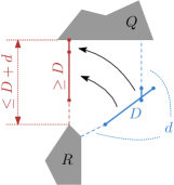
Figure 17: Barriers are bars with dots at endpoints. A subpath of a shortest $\mathcal{B}$-$\mathcal{T}$ path, going between two holes and not using edges of $G$ (blue), can be replaced by a shorter path (red) with the same barriers aligned along the edge of $G$.

Theorem 29.

Flow-HB1 can be solved in pseudopolynomial time.

Proof.

Let $K$ be the number of barriers. Similarly to the standard pseudopolynomial-time algorithms for bi-criteria shortest paths in graphs with two kinds of edge lengths (sometimes called weights and costs) [3], we propagate $K$ labels from $\mathcal{B}$; label $k=1\dots K$ of a vertex is the length of the shortest path from $\mathcal{B}$ to the vertex, using $k$ barriers. When propagating a label $l_{k}(u)$ along an edge $uv$ of length $L$, every label $i\geq k$ of $v$ is updated to the minimum of its current $i$th label $l_{i}(v)$ and $l_{k}(v)+\max[0,L-(i-k)]$, signifying the placement of $i-k$ barriers along $uv$. ∎

For a constant number of barriers we have:

Theorem 30.

Flow-HbD, and hence flow-hbD, flow-Hb1 and flow-hb1, are polynomial.

Proof.

Analogously to Theorem 27, only $O(1)$ super-barriers can be formed from a constant number of barriers. For each (constant-size) set of the super-barriers, there is a polynomial number of ways to place the super-barriers on edges of the critical graph (since $G$ has $O(h^{2})=O(n^{2})$ edges where $h$ is the number of holes in $P$); for each such placement the shortest $\mathcal{B}$-$\mathcal{T}$ path is computed, and the best overall placement is chosen. ∎

The remaining problem is flow-hB1:

Theorem 31.

Flow-hB1 is polynomial.

Proof.

With $O(1)$ holes, there are only $O(1)$ $\mathcal{B}$-$\mathcal{T}$ paths. For each $\mathcal{B}$-$\mathcal{T}$ path, we place the barriers greedily: First, we place $\lfloor L\rfloor$ barriers on each edge of length $L$ of the path (until we run out of the barriers) – this way we do not waste the barriers. Then, if any barriers remain and there is an edge of the path not yet fully covered by the barriers, we place one more barrier per edge, in decreasing order of the length of the part of the edge which is not yet covered. That is, we first place a barrier on the edge with the largest fractional part of the length (eating up as much of the remaining path length as possible), then on the edge with the second largest fractional part, etc. (this is optimal, since we waste as little total barrier length as possible). ∎

6 Conclusion

We introduced geometric versions of the graph-theoretic most vital arcs problem. We presented efficient solutions for simple polygons, and gave hardness results and algorithms for various versions of the problem. The most intriguing open problem is the hardness of path-hB1 (path blocking with few holes, our only unresolved version); we conjecture that it is polynomial, as still only a constant-number of super-barriers may be needed. Another interesting question is whether the flow and the path blocking have fundamentally different complexities: we proved that the complexities are the same for all versions except HB1 – for path-HB1 we showed weak hardness but lack a pseudopolynomial-time algorithm, while for flow-HB1 we have a a pseudopolynomial-time algorithm but no (weak) hardness proof. More generally, various other setups may be considered. For instance, one may be given a budget on the total length of the barriers– the problem then is how to split the budget between the barriers and where to locate them. For minimizing the maximum flow this version is easy: just place the barriers along the shortest $\mathcal{B}$-$\mathcal{T}$ path in the critical graph of the domain. For maximizing the shortest path in a simple polygon the solution is trivial: make a single barrier of the full length (and use our algorithm to find the optimal barrier location). Blocking shortest paths in polygons with holes in this setting is an open problem.

References

- [1] R. K. Ahuja, T. L. Magnanti, and J. B. Orlin. Network flows: theory, algorithms, and applications. Prentice hall, 1993.
- [2] D. L. Alderson, G. G. Brown, W. M. Carlyle, and L. A. Cox Jr. Sometimes there is no most-vital arc: assessing and improving the operational resilience of systems. Technical report, Naval Postgraduate School Monterey CA, 2013.
- [3] E. M. Arkin, J. S. Mitchell, and C. D. Piatko. Bicriteria shortest path problems in the plane. In Proc. 3rd Canad. Conf. Comput. Geom, pages 153–156, 1991.
- [4] M. O. Ball, B. L. Golden, and R. V. Vohra. Finding the most vital arcs in a network. Operations Research Letters, 8(2):73 – 76, 1989.
- [5] C. Bazgan, A. Nichterlein, and R. Niedermeier. A refined complexity analysis of finding the most vital edges for undirected shortest paths. In International Conference on Algorithms and Complexity, pages 47–60. Springer, 2015.
- [6] B. Chazelle. Triangulating a simple polygon in linear time. Discrete Comput. Geom., 6(5):485–524, 1991.
- [7] F. Chin, J. Snoeyink, and C. A. Wang. Finding the medial axis of a simple polygon in linear time. Discrete Comput. Geom., 21(3):405–420, 1999.
- [8] G. Citovsky, T. Mayer, and J. S. B. Mitchell. TSP with locational uncertainty: The adversarial model. In 33rd International Symposium on Computational Geometry, SoCG 2017, July 4-7, 2017, Brisbane, Australia, pages 32:1–32:16, 2017.
- [9] R. A. Collado and D. Papp. Network interdiction–models, applications, unexplored directions. Rutcor Res Rep, RRR4, Rutgers University, New Brunswick, NJ, 2012.
- [10] S. Eriksson-Bique, V. Polishchuk, and M. Sysikaski. Optimal geometric flows via dual programs. In Proceedings of the thirtieth Annual Symposium on Computational Geometry, page 100. ACM, 2014.
- [11] L. Gewali, A. Meng, J. S. B. Mitchell, and S. Ntafos. Path planning in weighted regions with applications. ORSA J. Comput., 2(3):253–272, 1990.
- [12] B. Golden. A problem in network interdiction. Naval Research Logistics (NRL), 25(4):711–713, 1978.
- [13] L. J. Guibas, J. Hershberger, D. Leven, M. Sharir, and R. E. Tarjan. Linear-time algorithms for visibility and shortest path problems inside triangulated simple polygons. Algorithmica, 2:209–233, 1987.
- [14] Q. Guo, B. An, and L. Tran-Thanh. Playing repeated network interdiction games with semi-bandit feedback. In Proceedings of the 26th International Joint Conference on Artificial Intelligence, IJCAI’17, pages 3682–3690. AAAI Press, 2017.
- [15] D.-S. Kim. Polygon offsetting using a Voronoi diagram and two stacks. Computer-Aided Design, 30(14):1069 – 1076, 1998.
- [16] K.-C. Lin and M.-S. Chern. Finding the most vital arc in the shortest path problem with fuzzy arc lengths. In Multiple Criteria Decision Making, pages 159–168. Springer, 1994.
- [17] M. Löffler. Existence and computation of tours through imprecise points. International Journal of Computational Geometry and Applications, 21(1):1–24, 2011.
- [18] S. H. Lubore, H. Ratliff, and G. Sicilia. Determining the most vital link in a flow network. Naval Research Logistics (NRL), 18(4):497–502, 1971.
- [19] E. A. Melissaratos and D. L. Souvaine. Shortest paths help solve geometric optimization problems in planar regions. SIAM Journal on Computing, 21(4):601–638, 1992.
- [20] J. S. Mitchell. On maximum flows in polyhedral domains. Journal of Computer and System Sciences, 40(1):88 – 123, 1990.
- [21] J. S. B. Mitchell. Geometric shortest paths and network optimization. In J.-R. Sack and J. Urrutia, editors, Handbook of Computational Geometry, pages 633–701. Elsevier, Amsterdam, 2000.
- [22] J. S. B. Mitchell and V. Polishchuk. Thick non-crossing paths and minimum-cost flows in polygonal domains. In SoCG, pages 56–65, 2007.
- [23] E. Nardelli, G. Proietti, and P. Widmayer. A faster computation of the most vital edge of a shortest path. Information Processing Letters, 79(2):81–85, 2001.
- [24] S. Neumayer, A. Efrat, and E. Modiano. Geographic max-flow and min-cut under a circular disk failure model. Computer Networks, 77:117–127, 2015.
- [25] C. Papadimitriou and M. Yannakakis. Shortest paths without a map. In Proc. 16th ICALP, pages 610–620, 1989.
- [26] R. Pollack, M. Sharir, and G. Rote. Computing the geodesic center of a simple polygon. Discrete & Computational Geometry, 4(6):611–626, Dec 1989.
- [27] H. D. Ratliff, G. T. Sicilia, and S. Lubore. Finding the n most vital links in flow networks. Management Science, 21(5):531–539, 1975.
- [28] J. C. Smith, M. Prince, and J. Geunes. Modern network interdiction problems and algorithms. In Handbook of combinatorial optimization, pages 1949–1987. Springer, 2013.
- [29] G. Strang. Maximal flow through a domain. Math. Program., 26:123–143, 1983.
- [30] P. Zhang and N. Fan. Analysis of budget for interdiction on multicommodity network flows. J. of Global Optimization, 67(3):495–525, Mar. 2017.