Single Stage DOA-Frequency Representation of the Array Data with Source Reconstruction Capability

Abstract

In this paper, a new signal processing framework is proposed, in which the array time samples are represented in DOA-frequency domain through a single stage problem. It is shown that concatenated array data is well represented in a $\mathbf{G}$ dictionary atoms space, where $\mathbf{G}$ columns correspond to pixels in the DOA-frequency image. We present two approaches for the $\mathbf{G}$ formation and compare the benefits and disadvantages of them. A mutual coherence guaranteed $\mathbf{G}$ manipulation technique is also proposed. Furthermore, unlike most of the existing methods, the proposed problem is reversible into the time domain, therefore, source recovery from the resulted DOA-frequency image is possible. The proposed representation in DOA-frequency domain can be simply transformed into a group sparse problem, in the case of non-multitone sources in a given bandwidth. Therefore, it can also be utilized as an effective wideband DOA estimator. In the simulation part, two scenarios of multitone sources with unknown frequency and DOA locations and non-multitone wideband sources with assumed frequency region are examined. In multitone scenario, sparse solvers yield more accurate DOA-frequency representation compared to some noncoherent approaches. At the latter scenario, the proposed method with group sparse solver outperforms some existing wideband DOA estimators in low SNR regime. In addition, sources’ recovery simultaneous with DOA estimation shows significant improvement compared to the conventional delay and sum beamformer and without prerequisites required in sophisticated wideband beamformers.

1 Introduction

Wideband signal processing is an active area of research in array processing. It has been studied extensively in areas such as radar, seismology, sonar, radio astronomy, speech acquisition and, acoustics [nordholm2014broadband, Reddy2012]. Although, the problem of direction-of-arrival (DOA) estimation has attracted considerable attention in array processing, representation of array data in DOA-frequency domain has not been directly examined. Certainly, any narrowband or wideband DOA estimation or source localization method without knowledge of the source’s frequency contents is impossible [VanTrees2002]. Furthermore, in real situations, a passive wideband array receives multiple sources with different bandwidths and center frequencies. Therefore, in non-cooperative scenarios, estimating the DOA-frequency distribution of the array data seems an inevitable pre-processing.

DOA estimation of wideband sources are essentially categorized into two different approaches; noncoherent and coherent. In noncoherent wideband processing, each subband is processed separately and the results are combined noncoherently. While in the coherent solution, DOA estimation is performed in a single center frequency. It combines the subbands covariance matrices coherently via a focusing matrix and the final covariance is used for DOA estimation[Wang1985]. Some advantages and drawbacks of them are listed below:

• Noncoherent approach suffers from intrinsic noncoherent losses.

• Increasing focusing errors with the bandwidth expansion makes the performance of coherent method worse than noncoherent one in ultra-wideband scenarios.

• The prerequisite of both solutions is the knowledge of frequency contents of the signal and dramatic performance degradation occurs in the case of incorporating noise only subbands in overall combination.

• Coherent methods require initial focusing angles, therefore, utilizing noncoherent pre-processing or DOA-frequency estimation is vital as the first step.

Some recent methods tried to overcome these problems. R-CSM [Sellone2006] proposed an iterative auto-focusing procedure to relax the requirement for initial DOA estimation. Test of orthogonality of projected subspaces (TOPS) [Yoon2006a] completely removed prerequisites of focusing procedure. It tests the orthogonality of the projected signal subspace and the noise subspace at each DOA and frequency subband, and, therefore, can be categorized in the noncoherent class. TOPS shows poor performance at high SNR levels and often leads to spurious peaks at all SNRs. Other algorithms were developed to improve TOPS, such as ETOPS [Zhang2010a], Squared-TOPS [Okane2010] and, WS-TOPS [Hayashi2016].

In parallel, some wideband array processing techniques exploiting the special structure of the antenna array have been developed. For example, [Chan2007] addresses frequency-invariant techniques for uniform concentric circular arrays (UCCAs) with omni-directional sensors and authors in [Liao2013a] extended that results for directional elements and with simpler array design procedure.

Sparse representation (SR) framework has also found new applications in DOA estimation during [Yang2017]. The fundamental work of Malioutov et al [malioutov2005sparse] named $\ell_{1}-$SVD and two recent works [Hu2014, Shen2017] are categorized in sparsity-based solution for DOA estimation of the wideband signals. Although, $\ell_{1}-$SVD is basically a narrowband solution, but have been extended to wideband situation by exploiting joint-sparsity in frequency-DOA domain. Authors in[Hu2014] used the idea proposed in [Shkolnisky2006] for approximating the band-limited signals with prolate spheroidal wave functions. It represented the array observations in a dictionary and applied block orthogonal matching pursuit (BOMP) to impose the sparsity only among bases with different delays. Recently, two time-domain solutions [liu2011direction, Hu2012a] for wideband DOA estimation employing SR have been proposed. They represent array covariance matrix in temporally delayed versions of source correlation function. This correlation function is assumed known in [Hu2012a] and can be estimated from observations in [liu2011direction].

In this paper, we propose a general framework to represent the array time samples directly in the space-frequency domain. It is named direct DOA-frequency representation (DDFR). The key difference between the proposed framework and most of the existing solutions in the wideband array processing is that unlike a two-phase approach (DOA estimation and then beamforming), DDFR solves the whole problem in a single stage, i.e., sources’ frequency content, spatial locations, and recovery coefficients are obtained by solving a single under-determined linear system. In other words, it is simultaneously an estimator and also a wideband beamformer.

The significant innovation of DDFR is the introduction of a $\mathbf{G}$ dictionary, by which the array multiple snapshots can be well represented in its atoms space. In other words, each column of $\mathbf{G}$ stands for a $(\theta,f)$ pixel in two-dimensional DOA-frequency image. Two approaches for $\mathbf{G}$ atoms arrangement are proposed and compared. It is shown that the first approach leads to a constant coherence among DOA-frequency atoms but their positions in DOA are uncontrolled. The second approach arranges atoms at desired $(\theta,f)$ points but there is no straightforward control over the dictionary coherence. We show that in noiseless case, DOA-frequency representation is formulated as a linear system in columns space of $\mathbf{G}$ . Regarding the problem size, number of snapshots and required DOA-frequency resolution, this linear system would yield an under-determined system, therefore has infinite solutions. Different solvers for this linear system are examined, including conventional minimum $\ell_{2}$-norm constraint and also sparsity-based penalty functions $\ell_{0}$ and $\ell_{1}$.

The solution of this system contains the DOA-frequency contents of the array data. One can use elements of the solution vector to reconstruct the source at a particular region in frequency or DOA. It means extending super-resolution capability into spatial filtering, which is absent in conventional and modern array processing techniques. For example, in a passive sonar array, one can listen to two adjacent sources and distinguish a marine mammal from a far passing ship. Furthermore, it can be utilized to show the power density of the array signal in DOA-frequency domain and estimate sources’ frequency contents for further processing.

Furthermore, in DDFR it is possible to impose sparsity only in the spatial domain, rather than in both DOA and frequency. It is necessary, especially when dealing with non-multitone wideband sources with known frequency band, such as chirp signals or band-limited Gaussian processes. In this case, the degree of freedom decreases and the problem reduces to group sparse form. Therefore, DDFR can act as a wideband DOA estimator when multiple non-multitone wideband sources with identical band exist. Briefly, DDFR framework does not suffer from previously mentioned noncoherent and coherent drawbacks, makes no assumption on the prior statistical information such as sources distribution or incoherence, does not involve subband processing and multiple eigenvalue decomposition (EVD), and in comparison with SR-based approaches enjoys excellent performance at low SNR regime and low number of snapshots with simultaneous beamforming feature. This special feature is obtained because the signal phase information is not lost through the estimation algorithm using DDFR.

The paper is organized as follows. Section 2 reviews the narrowband and wideband array signal model. Section 3 presents a brief introduction to the problem of sparse signal representation (SSR) and group sparse formulation. The main idea of DDFR and its related issues are presented in Section 4, and in Section LABEL:sec.Simulation the simulation results are examined for two scenarios of wideband signals. Finally, in Section LABEL:sec.Conclusion conclusions are drawn.

2 Signal Model

Let $s(t)$ denote a signal impinging on a linear array with $N_{S}$ sensors, located at $\theta$. The signal is received by sensors with different delays $\tau_{k}$. The delay $\tau_{k}$ is a function of the $k$’th sensor position and the source angle of arrival $\theta$. In the far-field situation, the observation vector $\mathbf{y}(t)$ containing all sensors data samples is,

$$\mathbf{y}(t)=\left[\begin{array}[]{c}s(t-\tau_{1})\\ \vdots\\ s(t-\tau_{N_{S}})\end{array}\right]\;,\qquad\tau_{k}=\frac{\mathbf{a}^{T}\mathbf{p}_{k}}{c}$$ (1)

where $\mathbf{a}$ is a unit vector describing source’s arrival direction, $\mathbf{p}_{k}$ is the $k$’th sensor position and $c$ is the wave propagation velocity in the medium [VanTrees2002]. For a uniform linear array aligned with $z$-axis and element distance $d$, the time delay due to $k$’th sensor is $\tau_{k}=-(k-1)d\sin(\theta)/c$.

2.1 Narrowband case

In narrowband case, the source $s(t)$ can be written as $s(t)=u(t)\exp(j2\pi f_{0}t)$, where $u(t)$ is the baseband signal with a bandwidth much smaller than the carrier frequency $f_{0}$. By this assumption, the delayed version of $s(t)$ is approximated with a phase shift. rl s(t-τ) =& u(t-τ)exp(j2πf_0(t-τ)) *
≈ u(t)exp(j2πf_0 t)exp(-j2πf_0τ)
= s(t)exp(-j2πf_0τ) By the equivalence of time delay to phase shift in (2.1), the measurement vector, in (1), for a single snapshot is reformulated as,

$$\mathbf{y}(t)=s(t)\left[\begin{array}[]{c}e^{-j2\pi f_{0}\tau_{1}(\theta)}\\ \vdots\\ e^{-j2\pi f_{0}\tau_{N_{S}}(\theta)}\end{array}\right]=s(t)\mathbf{v}(\theta,f_{0})$$ (2)

where $\mathbf{v}(\theta,f_{0})$ is called steering vector (or array manifold). Denoting $k$’th entry of the array manifold by $v_{k}(\theta,f_{0})=\exp(j\phi_{k})$ for $k\in\left\{1,\cdots,N_{S}\right\}$, $\phi_{k}$ is formulated as,

$$\phi_{k}=\left\{\IEEEeqnarraybox[][c]{r^{\prime}s}2\pi f_{0}(p_{k}/c)\sin(\theta)&generallineararray\\ 2\pi f_{0}(kd/c)\sin(\theta)uniformlineararray(ULA)\\ k\pi(f_{0}/f_{H})\sin(\theta)ULAwithd=(c/2f_{H})\right.$$ (3)

where $f_{H}$ is the observations upper frequency limit, $d$ is the elements distance, and $p_{k}$ is the $k$’th sensor position aligned with $z$-axis. If rewrite (2) for $K$ sources and in the presence of additive noise we will have, rCl y(t) &= [v(θ_1,f_0),⋯,v(θ_K,f_0)] [s_1(t)⋮s_K(t) ] + n(t)
= V_N_S ×K(Θ,f_0)s(t)_K×1 + n(t) where $\Theta=[\theta_{1},\cdots,\theta_{K}]^{T}$ is the sources direction of arrival (DOA) vector and $\mathbf{V}(\Theta,f_{0})$ is the steering matrix at $f_{0}$.

2.2 Wideband Case

In the wideband scenario, the equivalence between time delay and phase shift is no longer valid. We know that time delayed version of the signal has a Fourier transform pair as $s(t-\tau)\leftrightarrow S(f)e^{-j2\pi f\tau}$. In this situation, phase-shifts depends on the frequency as well as the source’s DOA. Therefore, the observation model (3) for the wideband case, is written at each frequency subband as,

$$\mathbf{y}(f)=\mathbf{V}(\Theta,f)\mathbf{s}(f)+\mathbf{n}(f)\$$ (4)

where $f\in\left\{f_{1},\cdots,f_{N_{F}}\right\}$ and $\Theta=[\theta_{1},\cdots,\theta_{N_{\theta}}]^{T}$.

3 Signal Sparse Representation (SSR)

The aim of sparse representation is to find a solution for a linear under-determined system with the minimum number of non-zero elements. Given an observation $\mathbf{y}\in\mathbb{C}^{M}$, and a dictionary matrix $\mathbf{D}\in\mathbb{C}^{M\times N}$ with $M<N$, we would like to find $\mathbf{x}\in\mathbb{C}^{N}$ that satisfies the linear system $\mathbf{y}=\mathbf{D}\mathbf{x}$ and has minimum non-zero elements. Denoting $\|\mathbf{x}\|_{0}$ as the number of non-zero entries of a vector $\mathbf{x}$, the sparsest solution of the above under-determined system is formulated as,

$$\underset{\mathbf{x}}{\min}\;\|\mathbf{x}\|_{0}\quad s.t.\quad\mathbf{y}=\mathbf{D}\mathbf{x}\quad(\ell_{0}\text{ problem})$$ (5)

The $\ell_{0}$ problem is combinatorial in nature, and the solution requires searching through all subsets of indices of $\mathbf{x}$. This is not tractable even for moderate values of $M$ and $N$ [Donoho2006]. The most common approximation is Basis Pursuit (BP) [chen2001atomic], which replaces $\ell_{0}$ with its closest convex norm $\ell_{1}$ :

$$\underset{\mathbf{x}}{\min}\;\|\mathbf{x}\|_{1}\quad s.t.\quad\mathbf{y}=\mathbf{D}\mathbf{x}\quad(\ell_{1}\text{ problem})$$ (6)

Extending the problem to noisy measurements case we have:

$$\underset{\mathbf{x}}{\min}\;\|\mathbf{x}\|_{1}\quad s.t.\quad\|\mathbf{y}-\mathbf{D}\mathbf{x}\|_{2}\leq\epsilon$$ (7)

where $\epsilon$ is an upper bound for noise, such that $\|\mathbf{n}\|_{2}\leq\epsilon$.

3.1 Group Sparsity

In some applications, sparsity exists among clusters of the $\mathbf{x}$ entries. It means the $\mathbf{x}$ vector is partitioned into $\mathcal{G}_{N}$ groups with either all zeros or all nonzeros elements, $\mathbf{x}=[\mathbf{x}_{\mathcal{G}_{1}}^{T},\mathbf{x}_{\mathcal{G}_{2}}^{T},\cdots,\mathbf{x}_{\mathcal{G}_{N}}^{T}]^{T}$. The group sparsity of $\mathbf{x}$ can be measured by an $\ell_{p,q}$ norm defined as [Hu2017],

$$\|\mathbf{x}\|_{p,q}\triangleq\left(\sum_{i=1}^{N}\|\mathbf{x}_{\mathcal{G}_{i}}\|_{p}^{q}\right)^{1/q}$$ (8)

where $p$ is the norm inside a group and $q$ is the norm among distinct groups. (7) can be expressed as a group sparse problem as,

$$\underset{\mathbf{x}}{\min}\;\|\mathbf{x}\|_{p,q}\quad s.t.\quad\|\mathbf{y}-\mathbf{D}\mathbf{x}\|_{2}\leq\epsilon\quad(\ell_{p,q}\text{ problem})$$ (9)

4 Direct DOA-Frequency Representation (DDFR)

First, direct representation of the array data in a $\mathbf{G}$ dictionary column space will be formulated. This acts as a $t\mapsto[f,\theta]$ transform, which gets the array time samples and results in a 2D image in frequency-DOA through a single stage formulation. Meanwhile, a simple solution for construction of the $\mathbf{G}$ dictionary, named constant $\Delta\delta$ approach, is derived. Then, a closed-form expression for the $\mathbf{G}$ atoms is found. This leads to a second dictionary design approach, named direct synthesis. In the next part, the mutual coherence of the $\mathbf{G}$ dictionary is calculated and a guaranteed $\mathbf{G}$ manipulation method is proposed. Finally, source reconstruction procedure is presented.

Let $M$ be the number of snapshots and $\mathbf{t}=\left[t_{1},\cdots,t_{M}\right]^{T}$ denote the sampling time vector. By arranging the array snapshots $\mathbf{y}(t)$, defined in (1), in a matrix form, the array observation matrix $\mathbf{Y}_{M\times N_{S}}$ is obtained as,

$$\mathbf{Y}=\left[\mathbf{y}(t_{1}),\cdots,\mathbf{y}(t_{M})\right]^{T}$$ (10)

where the columns of $\mathbf{Y}$ correspond to sensors’ temporal samples. Denoting $\mathbf{Y}(:,n)$ as the $n$’th column of $\mathbf{Y}$, $\mathbf{Y}(:,n)$ can be linearly represented in the Fourier bases space as follows:

$$\mathbf{Y}(:,n)=\sum_{k=1}^{N_{F}}x_{k}\mathbf{d}_{k}=\mathbf{D}(\mathcal{F})\mathbf{x}_{n}$$ (11)

where $\mathbf{x}_{n}$ is the signal representation coefficients of the $n$’th sensors observations and $\mathbf{D}=[d_{i,k}]$ is Fourier dictionary containing $N_{F}$ bases selected from $\mathcal{F}=\{f_{1},\cdots,f_{N_{F}}\}$ where

$$d_{i,k}=\frac{1}{\sqrt{M}}\exp\left(j2\pi f_{k}t_{i}\right)$$ (12)

Rewriting (11) in matrix form we have,

$$\mathbf{Y}=\mathbf{D}(\mathcal{F})\mathbf{X}$$ (13)

where $x_{i,j}$ is the coefficient corresponding to the frequency $f_{i}$ in the representation of the $j$-th sensor signal. Therefore, the $k$’th row of $\mathbf{X}$ is the array snapshot in the $f_{k}$ frequency. Accordingly, (4) holds for each row of the matrix $\mathbf{X}$. By denoting $\mathbf{X}(k,:)$ as the $k$’th row of $\mathbf{X}$,

$$\mathbf{X}(k,:)^{T}=\mathbf{V}(\Theta,f_{k})\mathbf{Z}(k,:)^{T}\quad k\in\left\{1,\cdots,N_{F}\right\}$$ (14)

where $\mathbf{Z}(k,:)$ denotes the array snapshot in the $k$’th subband. Since the array manifold matrix $\mathbf{V}(\Theta,f_{k})$ is a function of frequency as well as DOA, (14) is always examined separately in different subbands. This is the main hindrance that forces wideband array processing techniques to apply subband processing as a prerequisite. To resolve this problem, we rewrite steering vector as function of $\delta\triangleq f\sin(\theta)$ rather than $\theta$ or $f$. Assume $f_{L}\leq|f|\leq f_{H}$ and $\theta\in[-90^{\circ},+90^{\circ}]$, then $|\delta|\leq f_{H}$. By this change of variable, we can rewrite steering matrix as a function of $\delta$ as,

$$\mathbf{V}(\Delta)=\left[\mathbf{v}(\delta_{1}),\cdots,\mathbf{v}(\delta_{N_{D}})\right]_{N_{S}\times N_{D}}$$ (15)

where $\Delta=\left[\delta_{1},\cdots,\delta_{N_{D}}\right]^{T}$, $N_{D}$ is the number of $\delta$ grid points and each steering vector $\mathbf{v}(\delta_{i})$ isdefined as,

$$\mathbf{v}(\delta_{i})=\exp\left\{j2\pi\delta_{i}\frac{\mathbf{p}}{c}\right\}\>,\;\quad i\in\left\{1,\cdots,N_{D}\right\}$$ (16)

For linear array, $\mathbf{p}$ is array element position vector $\mathbf{p}=\left[p_{1},\cdots,p_{N_{S}}\right]^{T}$. Note that although $\Delta$ set leads to different DOA grid points at each $f_{i}$, it forms an identical steering vector matrix for the whole band. In other words, exploiting $\mathbf{V}(\Delta)$ in lieu of $\mathbf{V}(\Theta,f_{i})$, would generate DOA grid points with identical steering matrix at all bands but with different spatial grid map. Rewriting (14) in matrix form and with replacing new steering matrix $\mathbf{V}(\Delta)$, we have,

$$\mathbf{X}^{T}=\mathbf{V}(\Delta)\mathbf{Z}^{T}$$ (17)

and substituting (17) in (13) yields,

$$\mathbf{Y}=\mathbf{D}(\mathcal{F})\mathbf{Z}\mathbf{V}(\Delta)^{T}$$ (18)

where $\mathbf{Z}_{N_{F}\times N_{D}}=[z_{i,j}]$ is the DOA-frequency representation matrix and $z_{i,j}$ corresponds to $(f_{i},\delta_{j})$ which is uniquely mapped to $(f_{i},\theta_{j})$:

$$(f_{i},\delta_{j})\Rightarrow\theta_{j}=\sin^{-1}(\frac{\delta_{j}}{f_{i}})$$ (19)

obviously, if $|\frac{\delta_{j}}{f_{i}}|>1$ the corresponding $z_{i,j}$ does not map to a real $\theta_{j}$. Let $\mathcal{S}$ be the set of all invalid $(i,j)$ pairs as,

$$\mathcal{S}=\left\{(i,j)\left|\left|\frac{\delta_{j}}{f_{i}}\right|>1\right.\right\}\;\Rightarrow\quad z_{i,j\in\mathcal{S}}=0$$ (20)

Fig. 1 shows the mapping from $(f,\delta)$ to $(f,\theta)$. The $\theta$ values are labeled and iso-$\theta$ contour are shown with dashed lines. Indices belonging to $\mathcal{S}$ are illustrated with gray area. With uniform $\delta$ sampling, the invalid region possesses more grid points at lower frequencies, and this will lead to a frequency dependent resolution in DOA. This issue is examined in succeeding sections.

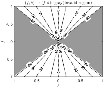
Figure 1: $(f,\delta)$ mapping to $(f,\theta)$. $f\in\left[-1,+1\right]$, $\delta\in\left[-1,+1\right]$. The labeled dashed lines illustrate the iso-$\theta$ cells.

Vectorizing (18), can simplify the equations. Since half of the $\mathbf{Z}$ matrix’s elements are zero, unacceptable entries would be removed simply in the vectorized form. For a given matrix $\mathbf{A}\in\mathbb{C}^{m\times n}$, $\mathbf{vec}(\cdot)$ operator is defined as,

$$\tilde{\mathbf{a}}_{mn\times 1}\triangleq\mathbf{vec}(\mathbf{A}_{m\times n})=\left[\mathbf{a}_{1}^{T},\cdots,\mathbf{a}_{n}^{T}\right]^{T}$$ (21)

where $\mathbf{a}_{k}$ denotes $k$’th column of $\mathbf{A}$. Applying $\mathbf{vec}(\cdot)$ to (18), we have,

$$\tilde{\mathbf{y}}=\mathbf{vec}(\mathbf{Y})=\mathbf{vec}(\mathbf{D}\mathbf{Z}\mathbf{V}^{T})=\left(\mathbf{V}\otimes\mathbf{D}\right)\mathbf{vec}(\mathbf{Z})=\mathbf{G}^{\prime}\tilde{\mathbf{z}}$$ (22)

where $\otimes$ stands for Kronecker Product. For $\mathbf{A}\in\mathbb{C}^{l\times n}$ and $\mathbf{B}\in\mathbb{C}^{p\times m}$ the Kronecker Product is defined as,

$$\mathbf{B}_{p\times m}\otimes\mathbf{A}_{l\times n}\triangleq\left[\begin{array}[]{ccc}b_{11}\mathbf{A}_{l\times n}&\cdots&b_{1m}\mathbf{A}_{l\times n}\\ \vdots&\ddots&\vdots\\ b_{p1}\mathbf{A}_{l\times n}&\cdots&b_{pm}\mathbf{A}_{l\times n}\end{array}\right]_{pl\times mn}$$ (23)

In (22), $\tilde{\mathbf{y}}$ is named the concatenated measurement vector, $\tilde{\mathbf{z}}$ is the resulting representation coefficients and $\mathbf{G}^{\prime}=\mathbf{V}\otimes\mathbf{D}$ is DOA-frequency dictionary. The $\mathbf{vec}(\cdot)$ operator should also be applied to $\mathcal{S}$ matrix as $\tilde{\mathbf{s}}=\mathbf{vec}(\mathcal{S})$. Therefore, (20) converts to $\tilde{z}_{k\in\tilde{\mathbf{s}}}=0$. This constraint is trivial since it can be applied directly to $\mathbf{G}^{\prime}$, by removing its invalid columns. Algorithm 1 shows a simple procedure to generate $\mathbf{G}$ from $\mathbf{G}^{\prime}$. In Algorithm 1, $\mathbf{G}$ is the final DOA-frequency dictionary and $\tilde{\mathbf{v}}_{f}$ and $\tilde{\mathbf{v}}_{\theta}$ are frequency and DOA grid points corresponding to columns of $\mathbf{G}$ , respectively. Thus, with $\mathbf{G}$ dictionary, the final DOA-frequency representation can be expressed as a linear system,

$$\tilde{\mathbf{y}}=\mathbf{G}\tilde{\mathbf{z}}$$ (24)

Algorithm 1 Make $\mathbf{G}$ dictionary with constant $\Delta\delta$ approach

1:function make_g_dic_delta($f_{L}$,$f_{H}$,$N_{F}$,$N_{D}$)

2:     $\mathbf{v}_{f}\leftarrow\left[f_{1},\cdots,f_{N_{F}}\right]^{T}$ $\triangleright$ $f_{L}\leq f\leq f_{H}$

3:     $\Delta\leftarrow\left[\delta_{1},\cdots,\delta_{N_{D}}\right]^{T}$ $\triangleright$ $|\delta|\leq f_{H}$

4:     make $\mathbf{D}_{M\times N_{F}}$ dictionary

5:     make $\mathbf{V}(\Delta)_{N_{S}\times N_{D}}$ $\triangleright$ see (16)

6:     $\mathbf{G}^{\prime}_{MN_{S}\times N_{F}N_{D}}\leftarrow\mathbf{V}\otimes\mathbf{D}$

7:     initialize $\mathcal{S}$ with $N_{F}\times N_{D}$ zero matrix

8:     initialize $\tilde{\mathbf{v}}_{f}$ and $\tilde{\mathbf{v}}_{\theta}$ with empty vector

9:     for $i\leftarrow 1,N_{F}$ do

10:         for $j\leftarrow 1,N_{D}$ do

11:              if $|\frac{\delta_{j}}{f_{i}}|\leq 1$ then

12:                  $\mathcal{S}(i,j)\leftarrow 1$

13:                  $\tilde{\mathbf{v}}_{f}\leftarrow\left[\tilde{\mathbf{v}}_{f},f_{i}\right]$

14:                  $\tilde{\mathbf{v}}_{\theta}\leftarrow\left[\tilde{\mathbf{v}}_{\theta},\sin^{-1}\left(\frac{\delta_{j}}{f_{i}}\right)\right]$

15:              end if

16:         end for

17:     end for

18:     Initialize $\mathbf{G}$ with empty matrix

19:     $\tilde{\mathbf{s}}\leftarrow\text{{vec}}(\mathcal{S})$

20:     for $k\leftarrow 1,N_{F}N_{D}$ do

21:         if $\tilde{s}_{k}=1$ then

22:              $\mathbf{G}\leftarrow\left[\mathbf{G}\>,\>\mathbf{g}_{k}^{\prime}\right]$ $\triangleright$ concatenate valid atoms

23:         end if

24:     end for

25:     Return $\tilde{\mathbf{v}}_{f},\tilde{\mathbf{v}}_{\theta},\mathbf{G}$

26:end function

The relation (24) is a fundamental result in wideband array processing. It shows that the concatenated measurement vector $\tilde{\mathbf{y}}$, lies in the columns space of the $\mathbf{G}$ dictionary. This can also be regarded as an extension of the narrowband model for wideband systems, since different frequencies can be incorporated in the array time signal recovery without any explicit Fourier analysis. This eliminates the subband processing for wideband signals and leads to a unified approach for narrowband and wideband scenarios.

4.1 $\mathbf{G}$ atoms formulation

In (24), it is shown that concatenated array time samples can be represented in the $\mathbf{G}$ columns space. In this section, we seek for the structure of $\mathbf{G}$ dictionary in more details. A closed-form relation for $\mathbf{g}(f,\theta)$ is found, consequently, in contrast to Algorithm 1 that there was no control on $\theta$ grid points, a direct $\mathbf{G}$ construction is presented in which arbitrary arrangement of $\mathbf{g}(f,\theta)$ atoms in $\theta$ and $f$ is provided.

To investigate the $\mathbf{G}$ matrix more closely, we refer to its definition in (22) and the Kronecker product (23). Assume $\mathbf{g}_{q}$ is the $q$’th column of $\mathbf{G}$ corresponding to $j$’th entry of $\mathcal{F}$, symbolized as $f_{j}$, and $r$’th element of $\Delta$, denoted as $\delta_{r}$. Denoting $\mathbf{G}$, $\mathbf{D}$ and $\mathbf{V}$ entries with $g,d$ and $v$ respectively, we have, rCl G_MN_S×N_F N_D &= [g_k,q] *
D_M×N_F = [d_i,j]
V_N_S×N_D = [v_e,r] Obviously,

$$g_{k,q}=v_{e,r}\cdot d_{i,j}$$ (25)

Due to definition of the Kronecker product, the following relations hold for subscripts, rCl”rCl i &= mod(k-1,M)+1 i∈{1,⋯,M }*
j = mod(q-1,N_F)+1 j∈{1,⋯,N_F }
e = ⌊k-1M⌋+ 1 e∈{1,⋯,N_S }
r = ⌊q-1NF⌋+ 1 r∈{1,⋯,N_D } Substituting (12) and (16) in (25) yields, rCl g_k,q &=exp{j2πδrcp_e }×1Mexp{j2πf_j t_i }
= 1M exp{j2πf_j( sin(θr)cp_e + t_i ) } It shows that the $q$’th column of $\mathbf{G}$ matrix is a pixel located at $(f_{j},\theta_{r})$ in DOA-frequency image, where $j$ and $r$ are calculated from (4.1) and (4.1) respectively. Now for a given $(f,\theta)$ we have the following step by step formulation for the DOA-frequency dictionary atom, denoted by $\mathbf{g}(f,\theta)$, rCl ~p_MN_S×1 &= vec((p_N_S×1×1_1×M)^T