Mapping the shape of the scalar potential with gravitational waves

Abstract

We study the dependence of the observable stochastic gravitational wave background induced by a first-order phase transition on the global properties of the scalar effective potential in particle physics. The scalar potential can be that of the Standard Model Higgs field, or more generally of any scalar field responsible for a spontaneous symmetry breaking in beyond-the-Standard-Model settings that provide for a first-order phase transition in the early universe. Characteristics of the effective potential include the relative depth of the true minimum ($E_{\alpha}^{4}$), the height of the barrier that separates it from the false one ($E_{m}^{4}$) and the separation between the two minima in field space ($v$), all at the bubble nucleation temperature. We focus on a simple yet quite general class of single-field polynomial potentials, with parameters being varied over several orders of magnitude. It is then shown that gravitational wave observatories such as aLIGO O5, BBO, DECIGO and LISA are mostly sensitive to values of these parameters in the region $E_{\alpha}\sim(0.1-10)\times E_{m}$. Finally, relying on well-defined models and using our framework, we demonstrate how to obtain the gravitational wave spectra for potentials of various shapes without necessarily relying on dedicated software packages.

I Introduction

The first detection of gravitational waves (GW) on Earth by the LIGO collaboration in 2016 Abbott et al. (2016) opened a new window to explore high-energy physics phenomena. One such source of gravitational radiation are first-order phase transitions (FOPT), which occur when a scalar field tunnels from a local minimum to a lower-lying true vacuum that is separated by an energy barrier Quiros (1999).

FOPTs proceed via the nucleation of bubbles of the stable true vacuum in the meta-stable false vacuum phase. The phase transition occurs at the temperature $T=T_{*}$ where bubbles of critical size can be formed; these critical bubbles expand, collide and ultimately thermalise by releasing their latent heat energy into the plasma formed of light particles.

The main frequency of the corresponding stochastic GW background grows with $T_{*}$. (Future experiments targeted at growing values of $T_{*}$ include LISA, BBO, DECIGO or aLIGO O5; see Ref. Moore et al. (2015) for details.) However, it is not yet clear how this frequency as well as the corresponding amplitude depend on the global properties of the scalar potential. We address this question in this paper.

To this aim, we focus on a class of polynomial functions parametrised by

$$V_{T_{*}}(\varphi)=\left[\left(\frac{\varphi}{c}\right)^{2}-a\right]^{2}+b\left(\frac{\varphi}{c}\right)^{3}~{},$$ (1)

describing the shape of the scalar potential density evaluated at the temperature $T_{*}$ where the phase transition happens. Let us emphasize that this functional form is merely a useful proxy that allows us to (numerically) trade the parameters $a$, $b$ and $c$ for the values of the vacuum expectation value (VEV) of $\varphi$ in the true minimum $v$, its depth $(E_{\alpha}^{4})$ and the energy barrier $(E_{m}^{4})$. Almost every potential can be well characterised by these parameters, as we demonstrate in subsequent sections; therefore our study does not restrict to Eq. (1) by any means.

The field $\varphi$ can be the Standard Model Higgs Zhang (1993); Grojean et al. (2005); Delaunay et al. (2008); Grinstein and Trott (2008); Harman and Huber (2016); Chala et al. (2018) or more generally any new other scalar field Schwaller (2015); Jaeckel et al. (2016); Addazi and Marciano (2018); Breitbach et al. (2018); Croon et al. (2018, 2019); Dev et al. (2019). Without loss of generality, the potential is finally shifted in order for the false minimum to lie at the origin; see Fig. 1.

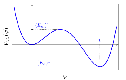
Figure 1: The scalar potential of a generic particle physics model with a FOPT. The potential is computed at the nucleation temperature $T_{*}$ where the nucleation rate $P$ to form bubbles of the true vacuum approaches $P\simeq 1$.

Because the main aim of this article is understanding how $T_{*}$ as well as other quantities relevant for the computation of the GW stochastic background depend on $v$, $E_{m}$ and $E_{\alpha}$, we compute the former parameters varying the later over several orders of magnitude. This procedure is explained in detail in Section II. For numerical calculations in this Section we rely predominantly on CosmoTransitions Wainwright (2012) and BubbleProfiler Athron et al. (2019) and cross-check these tools using the neural network method introduced in Ref. Piscopo et al. (2019).

We compute the actual GW signal in Section III, and discuss its dependence on the global properties of the potential. In Section IV we estimate the reach of different GW facilities, including LISA, DECIGO, BBO and aLIGO O5.

In Section V, we explain how to use our results to compute the GW spectrum in well-defined models of new physics. We validate this method by comparing to exact numerical integration of the action in each model. Finally, we offer conclusions in Section VI.

II Parametrisation of the effective potential

Our starting point is the effective potential $V_{T_{*}}(\varphi)$ in Eq. (1) that corresponds to a general particle physics model at the temperature $T=T_{*}$, where the model undergoes a FOPT. $T_{*}$ is the temperature of the formation of critical bubbles and is usually referred to as the nucleation temperature. In the unbroken phase, the VEV of $\varphi$ is vanishing, $\langle\varphi\rangle=0$, while in the broken phase it is non-zero, $\langle\varphi\rangle=v$.

Without loss of generality, we assume that the vacuum at the origin is the false minimum; the vacuum with the non-zero VEV being the true global one with vacuum energy $V_{T_{*}}(v)=-(E_{\alpha})^{4}<0.$ In total, the effective potential in Fig. 1 is characterised by three real-valued and positive parameters of mass-dimension one: the vacuum separation $v$, the vacuum energy change parameter $E_{\alpha}$, and the barrier height parameter $E_{m}$.

The value of the nucleation temperature is determined from the requirement that the probability ($P$) for a single bubble to nucleate within the horizon volume is of order one Moreno et al. (1998):

$$P(T_{*})\,=\,\int_{\infty}^{T_{*}}\frac{dT}{T}\,\left(\frac{2\zeta M_{\rm Pl}}{T}\right)^{4}\exp\left[-\frac{1}{T}\,S_{3}^{\,\rm cl}(T)\right]\simeq 1\,,$$ (2)

where $S_{3}^{\,\rm cl}(T_{*})$ is the action computed on the classical $O(3)$-symmetric bounce solution in the 3-dimensional theory with the potential $V_{T_{*}}(\varphi)$ Coleman (1977); Linde (1983). We have also defined $\zeta^{-1}=4\pi\sqrt{\pi g_{*}(T)/45}$. For the effective number of relativistic degrees of freedom in the plasma $g_{*}(T_{*})\sim 100$, we have $\zeta=0.03$. To allow the expression on the right-hand side of Eq. (2) to be of order one, the exponential suppression factor should be compensated by the large prefactor in Eq. (2):

$$\frac{1}{T_{*}}S_{3}^{\,\rm cl}(T_{*}) \,\simeq 4\log\left(0.06\frac{M_{\rm Pl}}{T_{*}}\right)$$

$$\,\simeq 140-4\log\frac{T_{*}}{100\,{\rm GeV}}\,.$$ (3)

For FOPTs at $T_{*}\sim 100$ GeV, the second term in the last equation can be neglected, leading to the usual approximation $S_{3}^{\,\rm cl}(T_{*})/T_{*}\sim 140$. We are however interested in FOPTs at arbitrarily large $T_{*}$, so we will take the full temperature dependence into account in what follows.

To optimise the scanning procedure over effective potentials with different global properties it is useful to introduce dimensionless variables by rescaling all physical parameters of the potential in Fig. 1 with respect to a single overall scale. A convenient choice for our purposes is the VEV $v$ of the global minimum.

We define:

$$\tilde{\varphi}(x)=\frac{\varphi(x)}{v}~{},\,\,\tilde{T}=\frac{T}{v}~{},\,\,\tilde{E}_{\alpha}=\frac{E_{\alpha}}{v}~{},\,\,\tilde{E}_{m}=\frac{E_{m}}{v}~{}.$$ (4)

Upon rescaling with $v$, the corresponding potential $\tilde{V}_{\tilde{T}_{*}}(\tilde{\varphi})$ is shown in Fig. 2 and is characterised now by two free parameters, $\tilde{E}_{\alpha}$ and $\tilde{E}_{m}$, with the minima fixed at $\tilde{\varphi}=0$ and $\tilde{\varphi}=1$.

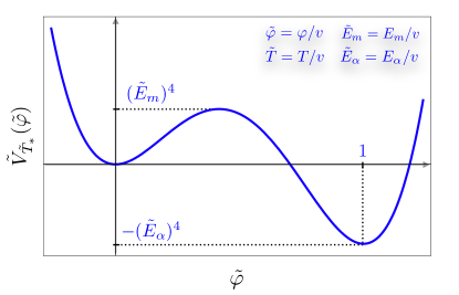
Figure 2: The effective potential in the rescaled variables.

For any given effective potential at the nucleation temperature $\tilde{T}_{*}$, we can now compute the value of $\tilde{T}_{*}$ using Eq. (3). To this end, we first need to find the $O(3)$-symmetric classical bounce solution that extremises the Euclidean action of the 3-dimensional theory with the potential $\tilde{V}_{\tilde{T}_{*}}(\tilde{\varphi})$,

$$\tilde{S}_{3}\,=\,4\pi\int dr\,r^{2}\left(\frac{1}{2}\tilde{\varphi}^{\,\prime}(r)^{2}+\tilde{V}_{\tilde{T}_{*}}(\tilde{\varphi})\right)\,,$$ (5)

by solving the classical equation Coleman et al. (1978),

$$\tilde{\varphi}^{\,\prime\prime}(r)+\frac{2}{r}\tilde{\varphi}^{\,\prime}(r)\,=\,\partial_{\tilde{\varphi}}\tilde{V}_{\tilde{T}_{*}}(\tilde{\varphi})\,.$$ (6)

We use custom routines based on BubbleProfiler Athron et al. (2019) to this aim. We subsequently compute the action on this classical bounce solution, $\tilde{S}_{3}^{\,\rm cl}$, and finally impose the bound of Eq. (3) to find

$$\frac{{\tilde{S}_{3}^{\,\rm cl}}}{\tilde{T_{*}}}\simeq 140-4\log\frac{\tilde{T}_{*}}{100}-4\log\frac{v}{\text{GeV}}\,.$$ (7)

We determine the nucleation temperature $T_{*}$ by solving (numerically) Eq. (7). This is the first of the three main parameters we need to obtain the stochastic GW spectrum generated in the FOPT.

The second parameter affecting the GW spectrum is the latent heat $\alpha$. It is defined as the ratio of the energy density released in the phase transition to the energy density of the radiation bath in the plasma:

$$\alpha=\,\frac{\rho_{\rm vac}}{\rho_{\rm rad}}=\frac{{E}_{\alpha}^{4}}{g_{*}(T_{*})\,\pi^{2}\,T_{*}^{4}/30}\,\simeq\,0.03\,\left(\frac{\tilde{E}_{\alpha}}{\tilde{T}_{*}}\right)^{4}.$$ (8)

The third quantity we need is $\beta/H_{*}$, characterising the speed of the phase transition:

$$\frac{\beta}{H_{*}}\,=\,T_{*}\frac{d}{dT}\left(\frac{1}{T}\,S_{3}^{\,\rm cl}(T)\right)_{T=T_{*}}.$$ (9)

In this equation, $H_{*}$ represents the Hubble constant at the time when $T=T_{*}$. A strong GW signal results from a slow phase transition with a large latent heat release, i.e. in the small $\beta/H_{*}$ and large $\alpha$ regime.

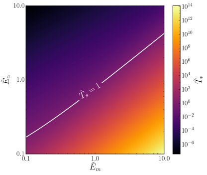
Figure 3: Values of $\tilde{T}_{*}$ as a function of $\tilde{E}_{m}$ and $\tilde{E}_{\alpha}$ in the range $[0.1,10.0]$. Note that since the potential density $V_{T}(\varphi)$ depends on the fourth power of $\tilde{E}_{m}$ and $\tilde{E}_{\alpha}$, the resulting variation of the shape of the potential is over eight orders of magnitude.

To determine $\beta/H_{*}$ from Eq. (9), we need to know the slope of the classical action $S_{3}^{\,\rm cl}(T)$ at $T=T_{*}$, and hence we need to compute infinitesimal deviations of the effective potential $V_{T}(\varphi)$ from its value at the nucleation temperature. One could use the full temperature-dependent expression for the effective potential, at 1-loop level Dolan and Jackiw (1974),

$$\Delta V_{T} =V_{T}-V_{T=0}$$ (10)

$$=\frac{T^{4}}{2\pi^{2}}\sum_{i}\pm n_{i}\int_{0}^{\infty}\mbox{d}q\,q^{2}\log\bigg{[}1\mp e^{-\sqrt{q^{2}+m_{i}^{2}(\varphi)/T^{2}}}\bigg{]},$$

but this approach would require us to specify the details of the mass spectrum $m_{i}(\varphi)$ and of the number of degrees of freedom $n_{i}$ in the microscopic theory. To retain a large degree of model-independence for our considerations, we use instead the leading-order Taylor expansion approximation, which is fully justified at high temperatures $T_{*}>\varphi$:

$$V_{T}(\varphi)\,=\,V_{T_{*}}(\varphi)\,+\,a_{T}\,(T^{2}-T_{*}^{2})\,\varphi^{2}\,.$$ (11)

There is just a single new parameter $a_{T}$ on the right-hand side of Eq. (11) that incorporates all model-dependence and characterises the deviations of $T$ from $T_{*}$ for different models. For any specific model the value of $a_{T}$ can be obtained upon expanding Eq. (10) to the order $T^{2}\varphi^{2}$ in the high-temperature expansion, $m_{i}(\varphi)^{2}/T_{*}^{2}<1$. This gives:

$$a_{T}\,=\,\frac{1}{24}\,\sum_{b,f}(n_{b}+n_{f}/2)\,,$$ (12)

where the sum is over bosonic and fermionic degrees of freedom.

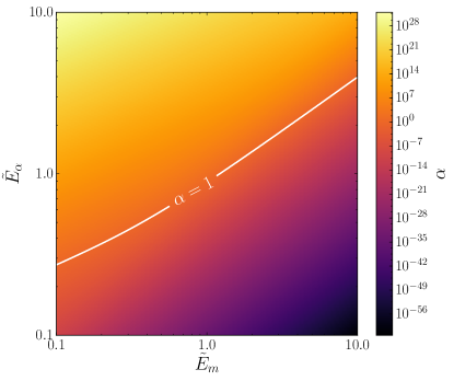
Figure 4: Values of $\alpha$ as a function of $\tilde{E}_{m}$ and $\tilde{E}_{\alpha}$ in the range $[0.1,10.0]$.

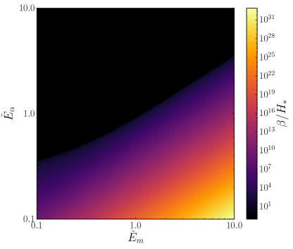
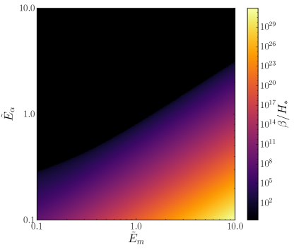
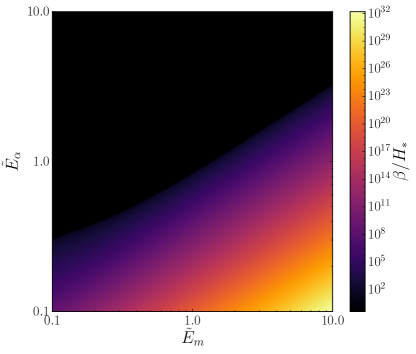
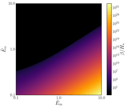
Figure 5: Values of $\beta/H_{*}$ as a function of $\tilde{E}_{m}$ and $\tilde{E}_{\alpha}$ in the range $[0.1,10.0]$ for different values of $a_{T}$. From top to bottom and left to right we show $a_{T}=1,0.1,0.2$ and $0.5$.

The validity of the high-temperature approximation assumed in Eq. (11) is easy to check. It is equivalent to requiring ${T}_{*}>v$, namely

$$\tilde{T}_{*}>1\,.$$ (13)

Thus, for any shape of the effective potential at $\tilde{T}_{*}$, e.g. that plotted in Fig. 2, the expression for the effective potential at general $\tilde{T}$ in (11) is justified when Eq. (13) holds.

In summary, to obtain $\beta/H_{*}$, we need to find the bounce solution in the theory with the effective potential (we now use the dimensionless variables),

$$\tilde{V}_{\tilde{T}}(\tilde{\varphi})\,=\,V_{\tilde{T}_{*}}(\tilde{\varphi})\,+\,a_{T}\,(\tilde{T}^{2}-\tilde{T}_{*}^{2})\,\tilde{\varphi}^{2}\,,$$ (14)

compute the 3D action on the bounce, $\tilde{S}_{3}^{\,\rm cl}(\tilde{T})$, and finally evaluate,

$$\frac{\beta}{H_{*}}\,=\,\tilde{T}_{*}\frac{d}{d\tilde{T}}\left(\frac{1}{\tilde{T}}\,\tilde{S}_{3}^{\,\rm cl}(\tilde{T})\right)_{\tilde{T}=\tilde{T}_{*}}.$$ (15)

There are three free parameters in total characterising the temperature-dependent potential (13) and hence the classical action: $\tilde{E}_{\alpha}$, $\tilde{E}_{m}$ and $a_{T}$. From these we obtain the three key parameters for the GW spectrum: the nucleation temperature $T_{*}/v$, the latent heat $\alpha$ and the $\beta$ parameter using Eqs. (7), (8), (14) and (15).

The values of $T_{*}/v$ in the plane $(\tilde{E}_{m},\tilde{E}_{\alpha})$ are plotted in Fig. 3. The region where $\tilde{T}_{*}=1$ is also shown by the white solid line. Below this line, $\tilde{T}_{*}>1$, therefore $T_{*}>v$ and hence the high-temperature approximation for computing $\beta/H_{*}$ as written in Eq. 15 holds.

We show the values of $\alpha$ in the same plane in Fig. 4. Analogously, in Fig. 5 we depict the values of $\beta/H_{*}$ in the same plane for four different choices of $a_{T}$. From top to bottom and left to right we have $a_{T}=1,\,0.1,\,0.2$ and $0.5$. In the black area, the high-temperature approximation fails. If in a specific model the temperature dependence is not quadratic, then $\beta/H_{*}$ cannot be estimated from the plots. Still, in such case one could consider the family of potentials parameterised by $\tilde{T}$ (equivalent to Eq. (14)), then for each case read $\tilde{S}_{3}^{\text{cl}}$ from Fig. 3 (roughly $\tilde{S}_{3}^{\text{cl}}\sim 140\,\tilde{T}_{*}$), and then take the corresponding derivative to compute $\beta/H_{*}$.

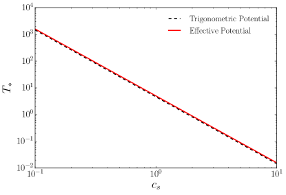
Figure 6: Value of $T_{*}$ as a function of $c_{s}$ in the model defined by Eq. 16 computed using the effective potential (solid red) and solving the bounce equation from scratch (dashed black).

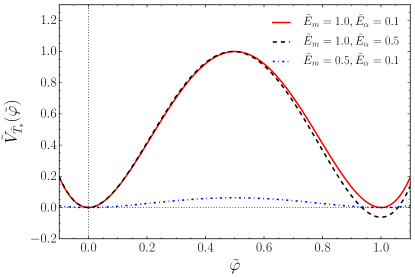
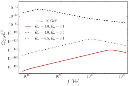
Figure 7: In the left panel we show the scalar potential for $\tilde{E}_{m}=1,\tilde{E}_{\alpha}=0.1$ (solid red); $\tilde{E}_{m}=1,\tilde{E}_{\alpha}=0.5$ (dashed black) and $\tilde{E}_{m}=0.5,\tilde{E}_{\alpha}=0.1$ (dashed-dotted blue) at $\tilde{T}_{*}$. (Note that the height of the barrier and the relative vacuum energy density depend on the fourth power of the parameters $\tilde{E}_{m}$ and $\tilde{E}_{\alpha}$.) The right panel shows the stochastic spectra of GWs produced in the course of the FOPTs for these choices of the scalar potential for $v=100$ GeV.

Finally, we test the robustness of our parametrisation of the potential by computing $T_{*}$ in a highly non-polynomial potential given by

$$V_{T}(h)=h\sin{(c_{s}h)}~{},$$ (16)

and comparing it to the result obtained by just plugging the values of $E_{m}$, $E_{\alpha}$ and $v$ (which depend on $c_{s}$) extracted from the expression (16) into our parametrisation in Eq. 1. The results are shown in Fig. 6. Notably, our method provides a reasonable estimate of the nucleation temperature also in this case, demonstrating that $E_{m}$ and $E_{\alpha}$ are the main global characteristics of the scalar potential. We have also checked that even nearly conformal potentials can be well described by these global characteristics. For example, we have studied the potential of a meson-like dilaton Bruggisser et al. (2018). Disregarding its mixing with the Higgs, it reads parametrically:

$$V(\chi)\sim a_{\chi}\chi^{4}-\epsilon(\chi)\chi^{4}~{},$$ (17)

with $\epsilon(\chi)\sim b_{\chi}(\chi/\chi_{0})^{\gamma}/[1-c_{\chi}(\chi/\chi_{0})^{\gamma}]$ the conformal breaking function and $a_{\chi}$, $b_{\chi}$, $c_{\chi}$, $\chi_{0}$ and $\gamma$ constants. For the case represented in the right panel of Fig. 6 in that reference, we have computed $\tilde{E}_{m}$ and $\tilde{E}_{\alpha}$, obtaining $\sim 0.18$ and $\sim 0.4$, respectively. Within our approach, this gives an action $S_{3}\sim 10066$ GeV. The authors of Ref. Bruggisser et al. (2018) use $S_{3}/T_{*}=140$ as the criteria to obtain $T_{*}$. Using the same criteria, we obtain therefore $T_{*}\sim 71.9$ GeV, while they report $T_{*}\sim 65.6$ GeV. This implies an error smaller than 10 %.

III Calculating the stochastic gravitational wave spectrum

Following Ref. Caprini et al. (2016), we estimate the stochastic GW background as the linear combination of three pieces:

$$h^{2}\Omega_{\text{GW}}\sim h^{2}\Omega_{\varphi}+h^{2}\Omega_{\text{sw}}+h^{2}\Omega_{\text{turb}}~{}.$$ (18)

The first component describes the contribution of the field $\varphi$ itself, due to the collisions of bubble walls after nucleation. Numerical simulations Huber and Konstandin (2008) suggest that it is approximately given by

$$h^{2}\Omega_{\varphi} \sim 1.67\times 10^{-5}$$ (19)

$$\times\mathcal{F}(2,2)\bigg{(}\frac{0.11v_{w}^{3}}{0.42+v_{w}^{2}}\bigg{)}\bigg{[}\frac{3.8\,(f/f_{\text{env}})^{2.8}}{1+2.8\,(f/f_{\text{env}})^{3.8}}\bigg{]}~{},$$

with

$$\mathcal{F}(x,y)=\bigg{(}\frac{H_{*}}{\beta}\bigg{)}^{x}\bigg{(}\frac{\kappa\alpha}{1+\alpha}\bigg{)}^{y}~{}\bigg{(}\frac{100}{g_{*}}\bigg{)}^{1/3}~{},$$ (20)

$f_{\text{env}}\sim 16.5\times 10^{-3}\,\text{mHz}\,[0.62/(1.8-0.1v_{w}+v_{w}^{2})]\,\mathcal{C}$, and $\mathcal{C}$ given by

$$\mathcal{C}=\bigg{(}\frac{\beta}{H_{*}}\bigg{)}\bigg{(}\frac{T_{*}}{100\,\text{GeV}}\bigg{)}\bigg{(}\frac{g_{*}}{100}\bigg{)}^{1/6}~{}.$$ (21)

We remind that $H_{*}$ and $g_{*}$ stand for the Hubble parameter and the number of relativistic degrees of freedom in the plasma at $T=T_{*}$, respectively. (Hereafter we will restrict to the regime where $\alpha\lesssim 1$, to avoid significant reheating, so that the temperature after the FOTP completes is indeed $\sim T_{*}$.) $v_{w}$ represents the bubble wall velocity and $\kappa$ the fraction of latent heat transformed into kinetic energy of $\varphi$.

The second term in Eq. 18 represents the GW background due to sound waves produced after the collision of bubbles and before the expansion dissipates the kinetic energy in the plasma. It comprises the dominant source of GW radiation. It approximately reads

$$h^{2}\Omega_{\text{sw}}\sim 2.65\times 10^{-6}$$ (22)

$$\times\mathcal{F}(1,2)\,v_{w}\,\bigg{(}\frac{f}{f_{\text{sw}}}\bigg{)}^{3}\bigg{(}\frac{7}{4+3\,(f/f_{\text{sw}})^{2}}\bigg{)}^{7/2}~{},$$

with $f_{\text{sw}}\sim 1.9\times 10^{-2}\,\text{mHz}\,(1/v_{w})\,\mathcal{C}$.

Finally, $h^{2}\Omega_{\text{turb}}$ is the magnetohydrodynamic turbulence formed in the plasma after the collision of bubbles:

$$h^{2}\Omega_{\text{turb}}\sim 3.35\times 10^{-4}$$ (23)

$$\times\mathcal{F}(1,3/2)v_{w}\bigg{\{}\frac{(f/f_{\text{turb}})^{3}}{[1+(f/f_{\text{turb}})]^{11/3}(1+8\pi f/h_{*})}\bigg{\}}~{},$$

with $f_{\text{turb}}\sim 2.7\times 10^{-2}\,\text{mHz}\,(1/v_{w})\,\mathcal{C}$ and $h_{*}$ being the redshifted Hubble time, $h_{*}=16.5\times 10^{-3}\,\text{mHz}\,T_{*}(g_{*}/100)^{1/6}/(100\,\text{GeV})$.

The bubble wall velocity $v_{w}$ is hard to estimate in general. It has been shown however that if the runaway condition $\alpha>\alpha_{\infty}\sim 4.9\times 10^{-3}/\tilde{T}_{*}^{2}$ is satisfied, then the bubble wall velocity is likely $v_{w}\sim 1$ Espinosa et al. (2010); Caprini et al. (2016). This happens in most of our parameter space. Moreover, the GW spectrum does not change dramatically in the allowed range of $v_{w}$ (conservative estimates suggest that $v_{w,\text{min}}>1/\sqrt{3}>0.5$ Steinhardt (1982)), so we fix $v_{w}\sim 1$ for simplicity. For $\kappa$, we take the fit Espinosa et al. (2010); Caprini et al. (2016)

$$\kappa\sim\alpha(0.73+0.083\sqrt{\alpha}+\alpha)^{-1}\,.$$ (24)

In Fig. 7, we show the GW stochastic background corresponding to different shapes of the potential at the nucleation temperature. We note that, for a barrier of fixed height, increasing the depth of the true vacuum shifts the spectrum to smaller frequencies (because it reduces $T_{*}$; see also Fig. 3) while it enhances the amplitude of the GW spectrum. The GW signal is also shifted to smaller frequencies and enhanced in amplitude if the barrier is decreased for a fixed value of the depth of the true vacuum, although the effect in this direction is less pronounced.

Clearly, reconstruction of the GW spectrum at future facilities (see Refs. Figueroa et al. (2018) for ongoing works at LISA) could shed light on the global properties of the scalar potential.

IV Limits from present and future gravitational wave experiments

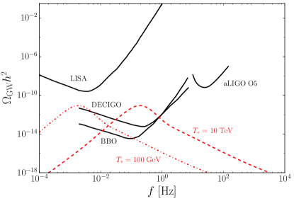
Figure 8: Sensitivity curves of LISA, DECIGO, BBO and aLIGO O5 to GWs as a function of the frequency. The predicted GW stochastic backgrounds for $\alpha=0.1$ and $\beta/H_{*}=100$ for $T_{*}=100$ GeV (dashed-dotted red curve) and $T_{*}=10$ TeV (dashed red curve) are also shown for comparison.

The sensitivity curves of different GW observatories are represented in Fig. 8. They are taken from the GW plotter http://rhcole.com/apps/GWplotter Moore et al. (2015), which is based on Ref. Sathyaprakash and Schutz (2009) (for LISA Bender et al. (2009)) and Ref. Yagi and Seto (2011) (for BBO Harry et al. (2006) and DECIGO Kawamura et al. (2006)). The GW stochastic background for $\alpha=0.1$ and $\beta/H_{*}=100$ is also plotted for comparison for $T_{*}=100$ GeV (dashed-dotted red curve) and $T_{*}=10$ TeV (dashed red curve). In order to address the reach of each of these facilities to the GW background originating from a FOPT with an effective potential at $T_{*}$ characterised by $E_{\alpha}$ and $E_{m}$, we proceed as follows. For each value of $v$ in the range $\sim$ 1 – $10^{6}$ GeV, we compute $E_{\alpha}$ and $E_{m}$ restricting to the region of $\tilde{E}_{m},\tilde{E}_{\alpha}\in[0.1,10]$ where $\alpha\lesssim 1$. We subsequently obtain, from the results above, the values of $\alpha$ and $\beta/H_{*}$ for $a_{T}=1$. We finally compare the GW spectrum as given by Eq. 18 with the sensitivity curves depicted in Fig. 8. We naively assume that, if the two curves overlap at any point in a fixed experiment, the latter can test the corresponding potential. Thus, for example, the GW spectrum represented by the dashed red curve in Fig. 8 would be observable by DECIGO and BBO but not by LISA or aLIGO O5. Let us also emphasize that we are neglecting the possible effects of having not “long-lasting” sound waves Ellis et al. (2018, 2019).

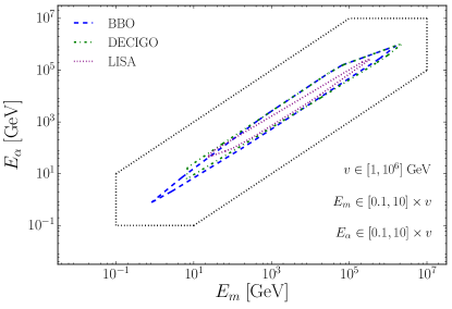
Figure 9: Regions of the plane $(E_{m},E_{\alpha})$ that can be probed by BBO (dashed blue), DECIGO (dashed-dotted green) and LISA (dotted purple) for $v$ in the range $[1,10^{14}]$ GeV. The dotted black box shows the region of the plane covered by the parameter scan.

The results are shown in Fig. 9. We note that BBO, DECIGO and LISA are mostly sensitive to the region $E_{\alpha}\sim(0.1-10)\times E_{m}$; the variations in magnitude between the different experiments being due to their different frequency reach. aLIGO O5 is sensitive to similar values, provided $v\gtrsim 10^{7}$ GeV, which is beyond the regime of applicability of Eq. (7).

To obtain the results displayed in this figure, we have scanned over the parameter ranges $E_{\alpha}\in[0.1,10]\times v$ and $E_{m}\in[0.1,10]\times v$ simultaneously. This region is depicted in Fig. 9 with the dotted black box. Thus, moving along the ellipsoid shape in Fig. 9 to larger and larger values of $E_{m}$ and $E_{\alpha}$, implies increasing the values of $v$. In other words, a larger value of $v$ has to be compensated by a deeper well of the potential to retain sensitivity at GW experiments. The region where $E_{\alpha}$ is small, and the potential barrier, expressed by $E_{m}$, is large, i.e. the lower right region of Fig. 9, becomes experimentally inaccessible.

The upper left region of Fig. 9, where the potential well is deep, i.e. $E_{\alpha}$ is large, and the barrier is small, would result in a very small value for the Euclidean action $\tilde{S}_{3}^{\,\rm cl}$ and, thus, according to Eq. 7, a very small nucleation temperature $T_{*}$. Such small $T_{*}$ would be formally unacceptable as it would invalidate our assumption of the high temperature approximation $T\gg v$ in Eq. 11. But even more importantly, the potential $V_{T}(\varphi)$ we consider is the result of a dynamical process when the plasma is cooling. Therefore, in realistic models, one would expect the phase transition to happen at temperatures much larger than that corresponding to the potential with the parameters in the upper left region of Fig. 9. Namely in a region closer to the ellipsoid shape in Fig. 9.

V Connection to fundamental theories

Our results do not only show the interplay between the global properties of the scalar potential and the GW stochastic background; they can be also used to compute the latter in an arbitrary model of new physics without necessarily solving for the bounce in Eq. 5 from scratch. To this aim, we provide tables with precomputed values of $\tilde{T}_{*}$, $\alpha$ and $\beta/H_{*}$ for varying $\tilde{E}_{m}$ and $\tilde{E}_{\alpha}$; see the webpage https://www.ippp.dur.ac.uk/~mspannow/gravwaves.html . Given this:

1. For fixed $T$ and $a_{T}$, one has to compute the finite-temperature effective potential in the corresponding model.

2. Subsequently, the values of $v$, $E_{\alpha}$ and $E_{m}$ are read off the effective potential. The values of $\tilde{E}_{\alpha}$ and $\tilde{E}_{m}$ can be trivially obtained from the former.

3. Next, one loops over all entries in the table with most similar $a_{T}$ provided in the link above. The triad $(\tilde{E}_{\alpha},\tilde{E}_{m},\tilde{T}_{*})$ from the table closest to the triad made out of the two values obtained in point 2 and $T/v$ should be taken.

4. The Euclidean distance between these two triads (normalised to the module of the latter), $d$, has to be computed.

5. Points $1-4$ are repeated for different values of $T$. The value of $T$ for which $d$ is smallest is taken as the estimated $T_{*}$. The estimated values for $\alpha$ and $\beta/H_{*}$ are those appearing in the row with most similar triad in the corresponding table.

We apply this process to a simple model given by

$$V_{T}(h)=-\frac{1}{2}\mu h^{2}+\frac{1}{4}\lambda h^{4}+\frac{c_{6}}{8\Lambda^{2}}h^{6}+a_{T}T^{2}h^{2}~{}.$$ (25)

This Lagrangian captures the modification on the Higgs potential due to new physics at a scale $\Lambda$ Grojean et al. (2005); Delaunay et al. (2008); Chala et al. (2018). For every $c_{6}/\Lambda^{2}$, we compute $\mu$ and $\lambda$ by requiring that the Higgs mass and the electroweak VEV match the measured values $m_{h}\sim 125$ GeV and $v_{\text{EW}}\sim 246$ GeV. We fix $a_{T}=1/32(4m_{h}^{2}/v_{\text{EW}}^{2}+3g^{2}+g^{\prime 2}+4y_{t}^{2}-12c_{6}v_{\text{EW}}^{2}/\Lambda^{2})$, with $g$ and $g^{\prime}$ the $SU(2)_{L}$ and $U(1)_{Y}$ gauge couplings, respectively, and $y_{t}$ the top Yukawa.

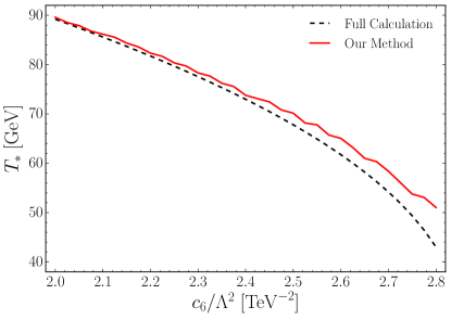
Figure 10: Value of $T_{*}$ as a function of $c_{6}/\Lambda^{2}$ in the model defined by Eq. 25 computed using the method outlined in the text (solid red) and solving the bounce equation from scratch (dashed black).

The value of $T_{*}$ as a function of $c_{6}/\Lambda^{2}$ obtained using the procedure outlined above is shown in Fig. 10. For comparison, we also show the value of $T_{*}$ obtained upon solving the bounce equation with BubbleProfiler in this particular model. The goodness of our method is apparent.

VI Conclusions and Outlook

We have computed the GW stochastic background produced in a FOPT triggered by the sudden change of VEV of a scalar field with potential characterised by given energy barrier $(E_{m}^{4})$ and depth of the true minimum $(E_{\alpha}^{4})$; see Fig. 1. We have shown that these parameters capture the most important and global characteristics of the scalar potential; the computation of the tunnelling rate, nucleation temperature, etc. being highly independent of other properties.

We have found that, for fixed values of $E_{m}$ ($E_{\alpha}$), the amplitude of the GW spectrum increases for growing (decreasing) $E_{\alpha}$ ($E_{m}$), with the frequency peak of the GW spectrum behaving conversely; GW observatories being mostly sensitive to the region $E_{\alpha}\sim(0.1-10)\times E_{m}$.

The reconstruction of the GW stochastic background at future facilities could therefore pinpoint the global structure of the Higgs potential, of which we only know its shape in a vicinity of the electroweak VEV. (Likewise for other scalar fields.) Thus, this study complements previous works in the literature aimed at characterising the nature of the Higgs potential using e.g. measurements of sphaleron energies Spannowsky and Tamarit (2017). Measurements of double Higgs production Dolan et al. (2013); No and Ramsey-Musolf (2014); Adhikary et al. (2018) instead can only reveal local properties of the Higgs sector. For example, the following simple potential

$$V(h)=\frac{m_{h}^{2}}{2}(h-v)^{2}+\frac{m_{h}^{2}}{2v}(h-v)^{3}+a_{4}(h-v)^{4}~{},$$ (26)

fullfills trivially $V^{\prime}(v)=0$, $V^{\prime\prime}(v)=m_{h}^{2}$ and $V^{\prime\prime\prime}(v)=3m_{h}^{2}/v$; exactly as in the Standard Model. However, it has a barrier at zero temperature for $a_{4}\sim 1/30$. In fact, assuming a $T$ dependence of the form $a_{T}T^{2}h^{2}$ with $a_{T}\sim 0.1$, the model undergoes a FOPT at $T_{*}\sim 10$ GeV.

Furthermore, as a bonus, we provide a method to use our results to estimate the main parameters entering the computation of the GW stochastic background, namely the nucleation temperature ($T_{*}$), the ratio of the energy density released in the phase transition to the energy density of the radiation bath ($\alpha$) and the inverse duration time of the phase transition ($\beta/H_{*}$). This method allows the user to avoid solving the bounce equations from scratch, and therefore it is on a similar footing with other dedicated tools such as CosmoTransitions Wainwright (2012) or BubbleProfiler Athron et al. (2019).

Acknowledgements.

This work is supported in part by an STFC Consolidated grant. MC is funded by the Royal Society under the Newton International Fellowship programme. MS is funded by the Humboldt Foundation and is grateful to the University of Tuebingen for hospitality during the finalisation of parts of this work.

References

- Abbott et al. (2016) B. P. Abbott et al. (LIGO Scientific, Virgo), Phys. Rev. Lett. 116, 061102 (2016), eprint 1602.03837.
- Quiros (1999) M. Quiros, in Proceedings, Summer School in High-energy physics and cosmology: Trieste, Italy, June 29-July 17, 1998 (1999), pp. 187–259, eprint hep-ph/9901312.
- Moore et al. (2015) C. J. Moore, R. H. Cole, and C. P. L. Berry, Class. Quant. Grav. 32, 015014 (2015), eprint 1408.0740.
- Zhang (1993) X.-m. Zhang, Phys. Rev. D47, 3065 (1993), eprint hep-ph/9301277.
- Grojean et al. (2005) C. Grojean, G. Servant, and J. D. Wells, Phys. Rev. D71, 036001 (2005), eprint hep-ph/0407019.
- Delaunay et al. (2008) C. Delaunay, C. Grojean, and J. D. Wells, JHEP 04, 029 (2008), eprint 0711.2511.
- Grinstein and Trott (2008) B. Grinstein and M. Trott, Phys. Rev. D78, 075022 (2008), eprint 0806.1971.
- Harman and Huber (2016) C. P. D. Harman and S. J. Huber, JHEP 06, 005 (2016), eprint 1512.05611.
- Chala et al. (2018) M. Chala, C. Krause, and G. Nardini, JHEP 07, 062 (2018), eprint 1802.02168.
- Schwaller (2015) P. Schwaller, Phys. Rev. Lett. 115, 181101 (2015), eprint 1504.07263.
- Jaeckel et al. (2016) J. Jaeckel, V. V. Khoze, and M. Spannowsky, Phys. Rev. D94, 103519 (2016), eprint 1602.03901.
- Addazi and Marciano (2018) A. Addazi and A. Marciano, Chin. Phys. C42, 023107 (2018), eprint 1703.03248.
- Breitbach et al. (2018) M. Breitbach, J. Kopp, E. Madge, T. Opferkuch, and P. Schwaller (2018), eprint 1811.11175.
- Croon et al. (2018) D. Croon, V. Sanz, and G. White, JHEP 08, 203 (2018), eprint 1806.02332.
- Croon et al. (2019) D. Croon, R. Houtz, and V. Sanz, JHEP 07, 146 (2019), eprint 1904.10967.
- Dev et al. (2019) P. S. B. Dev, F. Ferrer, Y. Zhang, and Y. Zhang, JCAP 1911, 006 (2019), eprint 1905.00891.
- Wainwright (2012) C. L. Wainwright, Comput. Phys. Commun. 183, 2006 (2012), eprint 1109.4189.
- Athron et al. (2019) P. Athron, C. Balázs, M. Bardsley, A. Fowlie, D. Harries, and G. White (2019), eprint 1901.03714.
- Piscopo et al. (2019) M. L. Piscopo, M. Spannowsky, and P. Waite, Phys. Rev. D100, 016002 (2019), eprint 1902.05563.
- John (1999) P. John, Phys. Lett. B452, 221 (1999), eprint hep-ph/9810499.
- Konstandin and Huber (2006) T. Konstandin and S. J. Huber, JCAP 0606, 021 (2006), eprint hep-ph/0603081.
- Masoumi et al. (2017) A. Masoumi, K. D. Olum, and B. Shlaer, JCAP 1701, 051 (2017), eprint 1610.06594.
- Akula et al. (2016) S. Akula, C. Balázs, and G. A. White, Eur. Phys. J. C76, 681 (2016), eprint 1608.00008.
- Jinno (2018) R. Jinno (2018), eprint 1805.12153.
- Espinosa (2018) J. R. Espinosa, JCAP 1807, 036 (2018), eprint 1805.03680.
- Espinosa and Konstandin (2019) J. R. Espinosa and T. Konstandin, JCAP 1901, 051 (2019), eprint 1811.09185.
- Guada et al. (2019) V. Guada, A. Maiezza, and M. Nemevšek, Phys. Rev. D99, 056020 (2019), eprint 1803.02227.
- Moreno et al. (1998) J. M. Moreno, M. Quiros, and M. Seco, Nucl. Phys. B526, 489 (1998), eprint hep-ph/9801272.
- Caprini et al. (2016) C. Caprini et al., JCAP 1604, 001 (2016), eprint 1512.06239.
- Coleman (1977) S. R. Coleman, Phys. Rev. D15, 2929 (1977), [Erratum: Phys. Rev.D16,1248(1977)].
- Linde (1983) A. D. Linde, Nucl. Phys. B216, 421 (1983), [Erratum: Nucl. Phys.B223,544(1983)].
- Coleman et al. (1978) S. R. Coleman, V. Glaser, and A. Martin, Commun. Math. Phys. 58, 211 (1978).
- Dolan and Jackiw (1974) L. Dolan and R. Jackiw, Phys. Rev. D9, 3320 (1974).
- Bruggisser et al. (2018) S. Bruggisser, B. Von Harling, O. Matsedonskyi, and G. Servant, JHEP 12, 099 (2018), eprint 1804.07314.
- Huber and Konstandin (2008) S. J. Huber and T. Konstandin, JCAP 0809, 022 (2008), eprint 0806.1828.
- Espinosa et al. (2010) J. R. Espinosa, T. Konstandin, J. M. No, and G. Servant, JCAP 1006, 028 (2010), eprint 1004.4187.
- Steinhardt (1982) P. J. Steinhardt, Phys. Rev. D25, 2074 (1982).
- Figueroa et al. (2018) D. G. Figueroa, E. Megias, G. Nardini, M. Pieroni, M. Quiros, A. Ricciardone, and G. Tasinato, PoS GRASS2018, 036 (2018), eprint 1806.06463.
- Sathyaprakash and Schutz (2009) B. S. Sathyaprakash and B. F. Schutz, Living Rev. Rel. 12, 2 (2009), eprint 0903.0338.
- Bender et al. (2009) P. Bender, A. Brillet, I. Ciufolini, A. Cruise, C. Cutler, K. Danzmann, F. Fidecaro, W. Folkner, J. Hough, P. McNamara, et al., MPQ Reports MPQ-233 (2009).
- Yagi and Seto (2011) K. Yagi and N. Seto, Phys. Rev. D83, 044011 (2011), [Erratum: Phys. Rev.D95,no.10,109901(2017)], eprint 1101.3940.
- Harry et al. (2006) G. M. Harry, P. Fritschel, D. A. Shaddock, W. Folkner, and E. S. Phinney, Class. Quant. Grav. 23, 4887 (2006), [Erratum: Class. Quant. Grav.23,7361(2006)].
- Kawamura et al. (2006) S. Kawamura et al., Class. Quant. Grav. 23, S125 (2006).
- Ellis et al. (2018) J. Ellis, M. Lewicki, and J. M. No (2018), [JCAP1904,003(2019)], eprint 1809.08242.
- Ellis et al. (2019) J. Ellis, M. Lewicki, J. M. No, and V. Vaskonen, JCAP 1906, 024 (2019), eprint 1903.09642.
- Spannowsky and Tamarit (2017) M. Spannowsky and C. Tamarit, Phys. Rev. D95, 015006 (2017), eprint 1611.05466.
- Dolan et al. (2013) M. J. Dolan, C. Englert, and M. Spannowsky, Phys. Rev. D87, 055002 (2013), eprint 1210.8166.
- No and Ramsey-Musolf (2014) J. M. No and M. Ramsey-Musolf, Phys. Rev. D89, 095031 (2014), eprint 1310.6035.
- Adhikary et al. (2018) A. Adhikary, S. Banerjee, R. K. Barman, B. Bhattacherjee, and S. Niyogi, JHEP 07, 116 (2018), eprint 1712.05346.