Small angle limits of Hamilton’s footballs

Yanir A. Rubinstein, Kewei Zhang
(May 2, 2019)
Abstract

Compact Ricci solitons on surfaces have at most two cone points, and are known as Hamilton’s footballs. In this note we completely describe the degenerations of these footballs as one or both of the cone angles approaches zero. In particular, we show that Hamilton’s famous non-compact cigar soliton is the Gromov–Hausdorff limit of Hamilton’s compact conical teardrop solitons.

1 Introduction

In this note we show that two seemingly very different Ricci solitons constructed by Hamilton are in fact closely related. Namely, we show that Hamilton’s non-compact steady Ricci soliton [8, p. 256], also known as the cigar soliton, is the Gromov–Hausdorff limit of compact shrinking Ricci solitons with a conical singularity constructed by Hamilton in the same foundational article [8, p. 261], also known as teardrop solitons. In fact, the cigar soliton turns out to be the blow-up limit of the teardrop solitons, and the limit takes place as the cone angle tends to zero. More generally, we describe all possible degenerations of Ricci solitons with at most two cone-points as the cone angles tend, possibly jointly, to zero.

This fits in nicely and is motivated by a conjectural picture put forward by Cheltsov and one of us [6, 12] in which non-compact Calabi–Yau fibrations emerge as the small angle limit of families of compact singular Einstein metrics known as Kähler–Einstein edge metrics. In fact, our result suggests this conjectural picture should extend to solitons and in a subsequent article we plan to pursue this [13]. Moreover, our result concretely illustrates the difficulty in treating divisors with more than one component and the ensuing joint small angle asymptotics.

1.1 Cigar as a limit of teardrops

As shown by Hamilton, there exists a soliton metric with a single conical singularity of angle $2\pi\beta$ on $S^{2}$ and area $2\pi(1+\beta)$ and such Kähler–Ricci solitons are nowadays known to be unique in any dimension [2] (below we will give an alternative uniqueness proof in this setting, see Remark 2.2). We denote this metric by $g_{\operatorname{TD},\beta}$ for each $\beta\in(0,1)$. Here, we consider $g_{\operatorname{TD},\beta}$ as a tensor on $\mathbb{R}^{2}\cong S^{2}\setminus\{\hbox{\rm cone point}\}$. On the other hand, Hamilton’s cigar soliton is the metric

$$g_{\operatorname{Cigar}}=\frac{dx\otimes dx+dy\otimes dy}{1+x^{2}+y^{2}}$$ (1)

on $\mathbb{R}^{2}$.

Theorem 1.1.

The cigar soliton on $\mathbb{R}^{2}$ is the pointed smooth (and hence also Gromov–Hausdorff) limit of rescaled conic teardrop solitons on $S^{2}$. More precisely, considered as tensors on $\mathbb{R}^{2}$, pointwise in every $C^{k}$-norm

$$g_{\operatorname{TD},\beta}/2\beta\;\buildrel{\beta\rightarrow 0}\over{\xrightarrow{\hskip 28.45274pt}}\;g_{\operatorname{Cigar}},$$

where $g_{\operatorname{TD},\beta}$ is the unique soliton metric of area $2\pi(1+\beta)$ with a single cone point of angle $2\pi\beta$ on $S^{2}$.

In fact, the proof of Lemma 2.4 gives that the rate of convergence in Theorem 1.1 is linear in $\beta$ in a certain coordinate chart.

1.2 Degenerations of footballs

In fact, Theorem 1.1 is a rather special case of a more general phenomenon that we now describe.

Let us work more generally with football solitons $g_{\operatorname{Foot},\beta_{1},\beta_{2}}$ that allow two cone points, namely one of angle $2\pi\beta_{1}$ at $N$ (the north pole) and one of angle $2\pi\beta_{2}$ at $S$ (the south pole). On the other hand, let us identify $\mathbb{R}^{2}$ with $S^{2}\backslash\{N\}$. The non-compact cone-cigar soliton of angle $2\pi\beta$ at the origin is given, in polar coordinates, by

$$g_{\operatorname{Cigar},\beta}=\frac{dr\otimes dr+\beta^{2}r^{2}d\theta\otimes d\theta}{1+r^{2}}$$ (2)

(in Remark 2.5 we show that this indeed solves the Ricci soliton equation). When $\beta=0$ we consider $g_{\operatorname{Cigar},0}$ as a metric on $\mathbb{R}_{+}$ (note that indeed the origin is at finite distance from any point). Note that $g_{\operatorname{Cigar}}=g_{\operatorname{Cigar},1}$ and $g_{\operatorname{TD},\beta_{1}}=g_{\operatorname{Foot},\beta_{1},1}$, so Theorem 1.1 is the case $\beta_{2}=1$ in the following:

Theorem 1.2.

The cone-cigar soliton on $\mathbb{R}^{2}$ or $\mathbb{R}_{+}$ (when $\beta>0$ or $\beta=0$, respectively) is the pointed smooth (and hence also Gromov–Hausdorff) limit of rescaled conic teardrop solitons on $S^{2}$. More precisely, considered as tensors on $\mathbb{R}^{2}\setminus\{0\}$, pointwise in every $C^{k}$-norm

$$\Big{(}S^{2},\frac{\beta_{2}}{2\beta_{1}}g_{\operatorname{Foot},\beta_{1},\beta_{2}},S\Big{)}\;\buildrel{\frac{\beta_{1}}{\beta_{2}}\rightarrow 0,\;\;\beta_{2}\rightarrow\beta}\over{\xrightarrow{\hskip 76.82234pt}}\;(\mathbb{R}^{2},g_{\operatorname{Cigar},\beta},0),$$

where $g_{\operatorname{Foot},\beta_{1},\beta_{2}}$ is the unique soliton metric on $S^{2}$ of area $2\pi(\beta_{1}+\beta_{2})$ with two cone points of angles $2\pi\beta_{1}<2\pi\beta_{2}$ at $N$ and $S$.

[Uncaptioned image]

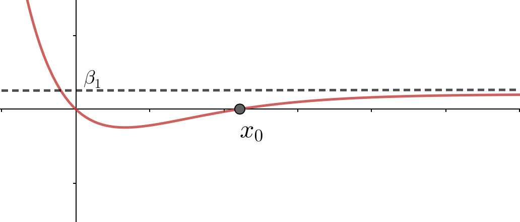
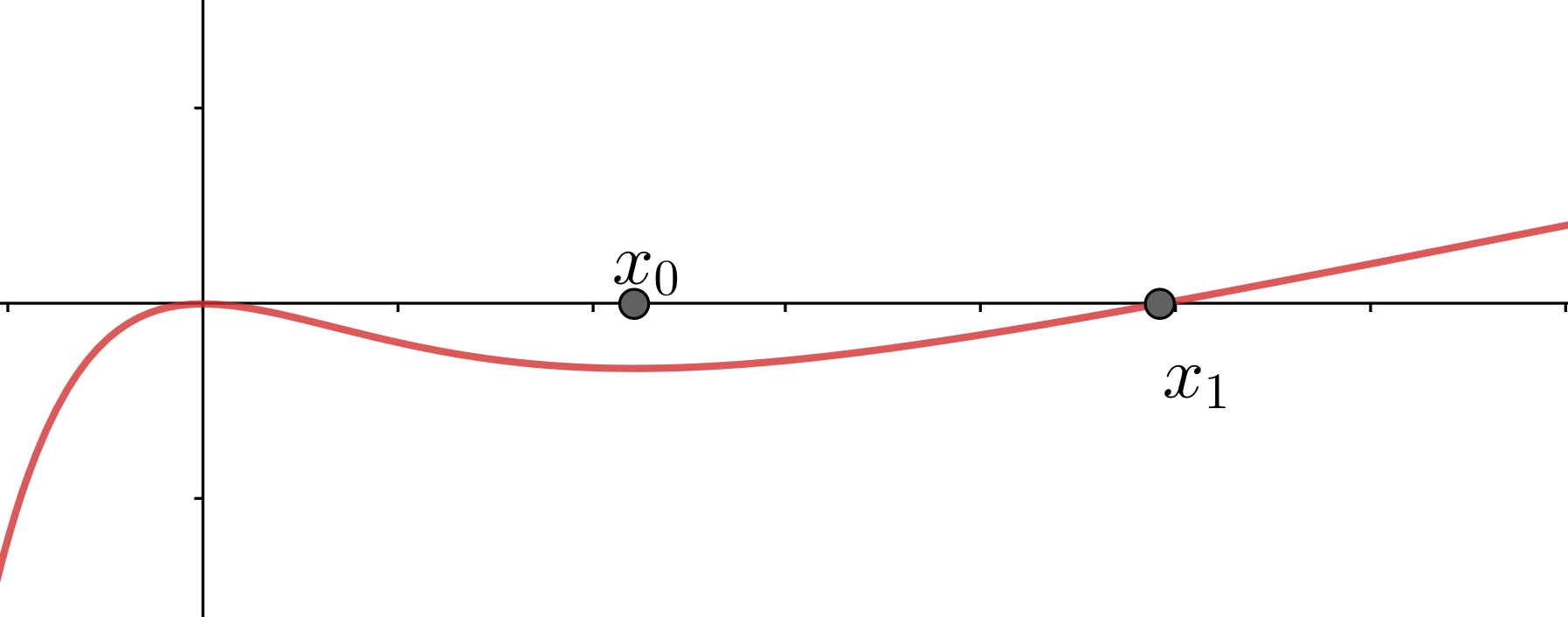
Theorem 1.2 describes joint degenerations of the cone angles with one converging to zero faster than the other (that may or may not converge to zero itself) and obtain a (possibly collapsed) cone-cigar in the jointly rescaled limit. Finally, we complete the picture by describing the asymptotic limit when both angles converge to zero at comparable speed (which can be considered as the hardest case, in a sense). Denote by

$$g_{\operatorname{Cyl}}:=\frac{dx\otimes dx+dy\otimes dy}{x^{2}+y^{2}},\quad(x,y)\in\mathbb{R}^{2}\setminus\{0\},$$

the pull-back of the flat metric on ${\mathbb{C}}$ to the cylinder ${\mathbb{C}}^{*}={\mathbb{C}}\setminus\{0\}$ under the map $z\mapsto\log z$.

Theorem 1.3.

Let $c\in(0,1)$. Considered as tensors on $\mathbb{R}^{2}\setminus\{0\}$, pointwise in every $C^{k}$-norm

$$\Big{(}\frac{1}{\beta_{1}^{2}}g_{\operatorname{Foot},\beta_{1},\beta_{2}},p_{\beta_{1},\beta_{2}}\Big{)}\;\buildrel{\frac{\beta_{1}}{\beta_{2}}\rightarrow c,\;\;\beta_{2}\rightarrow 0}\over{\xrightarrow{\hskip 76.82234pt}}\;(Cg_{\operatorname{Cyl}},e^{0}),$$

where $C=C(c)$, and where $g_{\operatorname{Foot},\beta_{1},\beta_{2}}$ is the unique soliton metric on $S^{2}$ of area $2\pi(\beta_{1}+\beta_{2})$ with two cone points of angles $2\pi\beta_{1}<2\pi\beta_{2}$ at $N$ and $S$, and $p_{\beta_{1},\beta_{2}}$ is the unique point in $\tau^{-1}(\beta_{1})\subset S^{2}$ with $\theta=0$ and $g_{\operatorname{Cyl}}$ is the flat cylinder metric on $\mathbb{R}^{2}\setminus\{0\}$.

Note that $p_{\beta_{1},\beta_{2}}$ is the unique point on the circle $\{\tau=\beta_{1}\}\subset S^{2}$ with $\theta=0$; this $\tau$-level set is characterized by the property that the region between the circle and the pole $N$ has area $\beta_{1}$ with respect to $g_{\operatorname{Foot},\beta_{1},\beta_{2}}$ (see Lemma 2.1 for more details on the $(\tau,\theta)$ coordinates).

We may summarize Theorems 1.11.3 in a succinct figure. The moduli space of footballs can be parametrized by the angle coordinates $(\beta_{1},\beta_{2})\in\mathbb{R}_{+}^{2}\setminus\{0\}$ where we represent each point $(\beta_{1},\beta_{2})$ by the unique Ricci soliton with cone angles $2\pi\beta_{1}$ at $N$ and $2\pi\beta_{2}$ at $S$ and of area $2\pi$ (unlike the normalization in the theorems above!). Then to describe the asymptotic behavior near the boundary of $\mathbb{R}^{2}_{+}$ it is most natural to blow-up the origin in $\mathbb{R}^{2}_{+}$ and use the coordinates $(r,\theta_{1}):=(\sqrt{\beta_{1}^{2}+\beta_{2}^{2}},\beta_{1}/\beta_{2})$ or $(r,\theta_{2}):=(\sqrt{\beta_{1}^{2}+\beta_{2}^{2}},\beta_{2}/\beta_{1})$:

[Uncaptioned image]

For example, in the joint limit $\beta_{1}/\beta_{2}\rightarrow 0,\;\beta_{2}\rightarrow 0$, Theorem 1.2 with $\beta=0$ translates to the area $2\pi(1+\beta_{1}/\beta_{2})\approx 2\pi$ metric $\frac{g_{\operatorname{Foot},\beta_{1},\beta_{2}}}{\beta_{2}}$ being asymptotic to $\frac{2\beta_{1}}{\beta^{2}_{2}}g_{\operatorname{Cigar},0}$ which in the projective coordinates $(r,\theta_{1})$ is asymptotic to $\frac{2\theta_{1}}{r}g_{\operatorname{Cigar},0}.$ The other arrows in the figure are obtained similarly from Theorems 1.11.3. In the language of [7, (1.2)] this gives a complete description of the boundary of the body of ample angles of the pair $(S^{2},N+S)$. A very intersting open problem is to generalize this to other pairs.

In the next section we begin by recalling Hamilton’s construction of the conical teardrop and football solitons, using slightly different language than his, namely the by-now-standard moment map picture going back to Calabi. The elementary proofs of Theorems 1.11.2 then follow by an asymptotic analysis of the resulting ordinary differential equations. In the final section we extend these arguments to the more difficult case of angles tending to zero with comparable speeds and prove Theorem 1.3.

2 Small angle asymptotics of footballs

In this section we prove Theorem 1.2 (that contains Theorem 1.1 as a particular case). We start by recalling some of the most pertinent details of the construction of the teardrop soliton on the unit sphere, due to Hamilton [8] (cf. Ramos [11]) but using the Calabi ansatz approach instead [5] (see also, e.g., [9]).

The Ricci soliton equation with two conical singularities is

$$\hbox{\rm Ric}\,\omega_{\beta_{1},\beta_{2}}=\omega_{\beta_{1},\beta_{2}}-\mathcal{L}_{X}\omega_{\beta_{1},\beta_{2}}+2\pi(1-\beta_{1})\delta_{N}+2\pi(1-\beta_{2})\delta_{S},$$ (3)

where $\omega_{\beta_{1},\beta_{2}}(\,\cdot\,,\,\cdot\,)=g_{\operatorname{Foot},\beta_{1},\beta_{2}}(J\,\cdot\,,\,\cdot\,)$ is the associated volume 2-form (where $J$ is the complex structure on $S^{2}$ considered as the Riemann sphere), $X$ is the soliton vector field (that will be determined later) and $\delta_{p}$ denotes the Dirac delta at $p$. In particular, applying cohomological considerations to this equation determines the area

$$\text{Vol}(S^{2},g_{\operatorname{Foot},\beta_{1},\beta_{2}})=2\pi(\beta_{1}+\beta_{2}).$$ (4)

The starting point is that the conical soliton metrics $g_{\operatorname{Foot},\beta_{1},\beta_{2}}$ (as, clearly, are also the $\theta$-indepedent $g_{\operatorname{Cigar},\beta_{2}}$) are rotationally symmetric [8, p. 258],[11, Lemma 3]. To see this one typically starts from the Riemannian definition of a Ricci soliton, on the smooth locus, as a solution of $2Kg=\hbox{\rm Ric}\,g=g-\nabla^{2}h$ from which it readily follows that $J\nabla h$ is a Killing vector for $g$, hence induces an $S^{1}$-symmetry. This then yields (3) with $X=\nabla h$. By the $S^{1}$-invariance, we see that, on $S^{2}\backslash\{N,S\}$, the volume 2-form $\omega_{\beta_{1},\beta_{2}}$ can be given by a potential function that only depends on $|z|$. Moreover, $\mathcal{L}_{X}\omega_{\beta_{1},\beta_{2}}=\sqrt{-1}\partial\bar{\partial}h$ with $h$ depending only on $|z|$ as well. So we set

$$s:=\log|z|^{2},$$ (5)

and write

$$\omega_{\beta_{1},\beta_{2}}=\sqrt{-1}\partial\bar{\partial}f(s),$$ (6)

where $f$ is a function to be determined (both $f$ and $h$ depend on $\beta_{1},\beta_{2}$ but we omit that from the notation).

In the following, we work only on the smooth part, namely

$$S^{2}\backslash\{S,N\}\cong\mathbb{C}^{*}.$$

On that chart we may use the holomorphic coordinate $w:=\log z$. Then, since $s=2{\operatorname{Re}}\,w$, $\frac{\partial}{\partial w}=\frac{1}{2}(\frac{\partial}{\partial s/2}-\sqrt{-1}\frac{\partial}{\partial{\operatorname{Im}}\,w})$, and as $f$ is independent of ${\operatorname{Im}}\,w,$

$$\omega_{\beta_{1},\beta_{2}}=\frac{\partial^{2}f}{\partial w\partial\bar{w}}\sqrt{-1}dw\wedge\overline{dw}=f^{\prime\prime}(s)\sqrt{-1}dw\wedge\overline{dw}=f^{\prime\prime}(s)\frac{\sqrt{-1}dz\wedge\overline{d{z}}}{|z|^{2}},$$ (7)

so $f$ must be a strongly convex function. Following Calabi, switch to the moment coordinate

$$\tau:=f^{\prime}(s),$$ (8)

and define a function $\varphi$ (depending on $\beta_{1},\beta_{2}$) on the image of the gradient of $f$ by

$$\varphi(\tau):=f^{\prime\prime}(s)$$ (9)

(simply the inverse of the second derivative of the Legendre transform of $f$). In the following, we seek an explicit formula for $\varphi(\tau)$ (see (25)) since the expression of $\varphi(\tau)$ can in turn give an explicit formula for the soliton metric. We start by rewriting the metric in terms of $\tau$.

Lemma 2.1.

The restriction of the metric $g_{\operatorname{Foot},\beta_{1},\beta_{2}}$ to $S^{2}\backslash\{S,N\}$ can be written as

$$g_{\operatorname{Foot},\beta_{1},\beta_{2}}=\frac{1}{2\varphi(\tau)}d\tau\otimes d\tau+2\varphi(\tau)d\theta\otimes d\theta,\qquad\tau\in(0,\beta_{1}+\beta_{2}),\quad\theta\in[0,2\pi).$$ (10)
Proof.

Using (7) and standard relations between Riemaniann, Hermitian, and Kähler metrics,

$$g_{\operatorname{Foot},\beta_{1},\beta_{2}}=\frac{2f^{\prime\prime}(s)}{r^{2}}(dr\otimes dr+r^{2}d\theta\otimes d\theta)$$

where we let $z=re^{i\theta}$. Recall from (5) that $r=e^{\frac{s}{2}}.$ Hence,

$$g_{\operatorname{Foot},\beta_{1},\beta_{2}}=\frac{f^{\prime\prime}(s)}{2}ds\otimes ds+2f^{\prime\prime}(s)d\theta\otimes d\theta.$$

Using (8)–(9),

$$ds=\frac{1}{\varphi}d\tau,$$ (11)

and using this and (9) again gives,

$$g_{\operatorname{Foot},\beta_{1},\beta_{2}}=\frac{1}{2\varphi(\tau)}d\tau\otimes d\tau+2\varphi(\tau)d\theta\otimes d\theta.$$

In particular, we see that the volume form of this metric is $d\tau\wedge d\theta.$ Here $\theta\in[0,2\pi)$ and $\tau$ belongs to an interval that we need to determine. Using (4),

$$\tau\in(c,c+\beta_{1}+\beta_{2}),$$

where $c$ is a constant (here is where we really needed the $2\pi$ factors in (3), otherwise we would get $2\pi$ factors in the domain of $\tau$). Note that here, we can simply choose $c$ to be 0. This is because we can add an affine function $-cs$ to $f(s)$ to shift the interval of $\tau$ without changing the metric. ∎

So in the following, we will use $\tau$ as our variable to search for an explicit expression for $\varphi(\tau)$ and convert the soliton equation to a simple ODE. First, recall from (6) that

$$\omega_{\beta_{1},\beta_{2}}=\sqrt{-1}\varphi dw\wedge\overline{dw}.$$ (12)

Similarly to (7), now using (11), the Ricci form is given by

$\displaystyle\hbox{\rm Ric}\,\omega_{\beta_{1},\beta_{2}}$ $\displaystyle=-\sqrt{-1}\partial\bar{\partial}\log\varphi$ (13)
$\displaystyle=-\sqrt{-1}\frac{\partial^{2}\log\varphi}{\partial s^{2}}dw\wedge\overline{d{w}}$
$\displaystyle=-\sqrt{-1}\frac{\partial}{\partial s}\Big{(}\frac{\varphi^{\prime}}{\varphi}\frac{d\tau}{ds}\Big{)}dw\wedge\overline{d{w}}$
$\displaystyle=-\sqrt{-1}\varphi^{\prime\prime}\frac{d\tau}{ds}dw\wedge\overline{d{w}}=-\sqrt{-1}\varphi\varphi^{\prime\prime}dw\wedge\overline{d{w}}.$

In particular, the Gaussian curvature is given by

$$K(S^{2},\omega_{\beta_{1},\beta_{2}})=-\varphi^{\prime\prime}(\tau).$$ (14)

Now we turn to the potential function $h$ of the soliton vector field. Recall that $h$ only depends on $s$, hence only on $\tau$ and we may write $h=h(\tau).$ Also recall that $h$ is a holomorphy potential, namely the dual of $\bar{\partial}h$ with respect to Hermitian metric,

$\displaystyle\nabla^{1,0}h$ $\displaystyle=\frac{1}{\varphi}\frac{\partial h(\tau)}{\partial\bar{w}}\frac{\partial}{\partial w}$
$\displaystyle=\frac{1}{\varphi}\frac{\partial h(\tau)}{\partial s}\frac{\partial}{\partial w}$
$\displaystyle=\frac{1}{\varphi}h^{\prime}(\tau)\frac{d\tau}{ds}\frac{\partial}{\partial w}$
$\displaystyle=h^{\prime}(\tau)\frac{\partial}{\partial w},$

is a holomorphic vector field (which happens to be $X-\sqrt{-1}JX$ in our earlier notation). This implies

$$h^{\prime}(\tau)=a\in\mathbb{R},\quad\tau\in(0,\beta_{1}+\beta_{2})$$

for some constant $a$ to be determined. So up to an irrelevant constant, we get

$$h(\tau)=a\tau.$$

Hence,

$\displaystyle\sqrt{-1}\partial\bar{\partial}h$ $\displaystyle=\sqrt{-1}a\frac{\partial^{2}\tau}{\partial s^{2}}dw\wedge\overline{dw}$ (15)
$\displaystyle=\sqrt{-1}a\frac{\partial\varphi(\tau)}{\partial s}dw\wedge\overline{dw}$
$\displaystyle=\sqrt{-1}a\varphi^{\prime}(\tau)\frac{d\tau}{ds}dw\wedge\overline{dw}$ $\displaystyle=\sqrt{-1}a\varphi\varphi^{\prime}dw\wedge\overline{dw}.$

Combining (12), (13) and (15), the Ricci soliton equation on the smooth locus reduces to

$$-\varphi^{\prime\prime}\varphi=\varphi-a\varphi^{\prime}\varphi,$$ (16)

and since $\varphi>0$ (by (9) and the convexity of $f$),

$$\varphi^{\prime\prime}(\tau)-a\varphi^{\prime}(\tau)+1=0.$$ (17)

Thus the soliton equation becomes an ordinary differential equation for $\varphi$. To solve it, let us determine the boundary conditions.

Remark 2.2.

Typically, the boundary conditions are declared by an ansatz and so one does not quite obtain uniqueness of the teardrop solitons in this method (instead relying, for the uniqueness on the general result of Berndtsson [2]). Here instead, we actually prove uniqueness by deriving the boundary conditions using the asymptotic expansion of [10].

Recall that, by Lemma 2.1, $\tau\in(0,\beta_{1}+\beta_{2}).$ By (11) $\tau$ increases as $s$ increases (which in turn increases as $|z|$ does). Thus $\{N\}=\{z=0\}=\{\tau=0\}$ and $\{S\}=\{z=\infty\}=\{\tau=\beta_{1}+\beta_{2}\}$. Since $\omega_{\beta_{1},\beta_{2}}$ has cone angle $2\pi\beta_{1}\in(0,2\pi)$ at $N$, it follows from [10, Theorem 1, Proposition 4.4] (as the Ricci soliton equation (3) is a complex Monge–Ampère equation of the form treated in op. cit.) that $f$ has a complete asymptotic expansion near $z=0$ whose leading term is $|z|^{2\beta_{1}}$:

$\displaystyle\varphi$ $\displaystyle\sim C_{1}+C_{2}|z|^{2\beta_{1}}+(C_{3}\sin\theta+C_{4}\cos\theta)|z|^{2}+O(|z|^{2+\epsilon})$
$\displaystyle=C_{1}+C_{2}e^{\beta_{1}s}+(C_{3}\sin\theta+C_{4}\cos\theta)e^{s}+O(e^{(1+\epsilon)s})$

(note that $r$ in [10, (56)] is equal to $|z|^{\beta_{1}}/\beta_{1}$ in our notation, see [10, p. 102]). From (11) (for instance) we see that $\varphi$ must vanish at $N$ (and $S$) since $\varphi>0$ away from $N$ and $S$ and $\tau$ lives in a bounded interval while $s$ lives on an unbounded one. Thus, $C_{1}=0$ (actually also $C_{3}=C_{4}=0$ as $\varphi$ is independent of $\theta$ but we do not need this). Moreover, the expansion can be differentiated term-by-term as $|z|\rightarrow 0$ or $s\rightarrow-\infty$. As $\varphi^{\prime}(\tau)=\frac{\partial\varphi}{\partial s}\frac{ds}{d\tau}=\frac{\partial\varphi}{\partial s}/\varphi,$ we obtain

$$\varphi(0)=0,\quad\varphi^{\prime}(0)=\beta_{1}.$$ (18)

The same arguments imply that

$$\varphi(\beta_{1}+\beta_{2})=0,\quad\varphi^{\prime}(\beta_{1}+\beta_{2})=-\beta_{2}.$$ (19)

Next, we claim that $\beta_{1}$ and $\beta_{2}$ determine $a$. Indeed, (17) is a first-order equation for $\tau$ and integrating it yields

$$a\varphi^{\prime}(\tau)=Ce^{a\tau}+1.$$ (20)

Using the boundary conditions we find

$$-(a\beta_{2}+1)e^{-a(\beta_{1}+\beta_{2})}=C=a\beta_{1}-1,$$ (21)

i.e.,

$$a\beta_{1}-1+(a\beta_{2}+1)e^{-a(\beta_{1}+\beta_{2})}=0.$$ (22)

As we will now show, this can be used to determine $a$ uniquely from $\beta_{1},\beta_{2}$, and, moreover, determines the asymptotic behavior of $a$ as $\beta_{1}/\beta_{2}\rightarrow 0$.

Lemma 2.3.

There is a unique $a=a(\beta_{1},\beta_{2})\in(0,\frac{1}{\beta_{1}})$ solving (22). Moreover,

$$\lim_{\frac{\beta_{1}}{\beta_{2}}\rightarrow 0}a(\beta_{1},\beta_{2})\beta_{1}=1.$$ (23)
Proof.

Note that $a\not=0$. Indeed, $a=0$ trivially satisfies (22) but then the soliton vector field vanishes and by (3) we have a metric of constant scalar curvature which forces $\beta_{1}=\beta_{2}$ [8, p. 261],[14, Theorem I], contrary to our assumption that $\beta_{1}<\beta_{2}$.

Put

$$F_{\beta_{1},\beta_{2}}(x)\equiv F(x):=\beta_{1}x-1+(x\beta_{2}+1)e^{-x(\beta_{1}+\beta_{2})}.$$ (24)

Compute,

$$F^{\prime}(x)=\beta_{1}-\big{(}\beta_{1}+x\beta_{2}(\beta_{1}+\beta_{2})\big{)}e^{-x(\beta_{1}+\beta_{2})},$$

Notice that $F(0)=F^{\prime}(0)=0$ and $F$ is asymptotically linear with slope $\beta_{1}$, and $\lim_{x\rightarrow\infty}F^{\prime}(x)=\beta_{1}$. Next,

$$F^{\prime\prime}(x)=\Big{[}(\beta_{1}+\beta_{2})\big{(}\beta_{1}+x\beta_{2}(\beta_{1}+\beta_{2})\big{)}-\beta_{2}(\beta_{1}+\beta_{2})\Big{]}e^{-x(\beta_{1}+\beta_{2})},$$

so $F^{\prime\prime}$ is initially negative (as $\beta_{1}<\beta_{2}$) and changes sign precisely once with $F^{\prime\prime}\Big{(}\frac{\beta_{2}-\beta_{1}}{\beta_{2}(\beta_{1}+\beta_{2})}\Big{)}=0$. Thus, $F^{\prime}$ vanishes for precisely one positive value $x_{0}$ of $x$ that is a local minimum for $F$ with $F(x_{0})<0$. Also, $F$ vanishes for precisely one positive value $x_{1}=x_{1}(\beta_{1},\beta_{2})$ of $x$ and $x_{1}>x_{0}$. Note $F(x_{1})=0$ means

$$\beta_{1}x_{1}-1=-(x_{1}\beta_{2}+1)e^{-x_{1}(\beta_{1}+\beta_{2})}<0,$$

i.e., $x_{1}\in(0,1/\beta_{1})$ as claimed.

Refer to caption
(a) $F^{\prime}(x)$
Refer to caption
(b) $F(x)$

Finally, fix $\epsilon\in(0,1)$. Then,

$\displaystyle F\big{(}(1-\epsilon)/\beta_{1}\big{)}$ $\displaystyle=-\epsilon+\big{(}(1-\epsilon)\beta_{2}/\beta_{1}+1\big{)}e^{-(1-\epsilon)(\beta_{1}+\beta_{2})/\beta_{1}}$
$\displaystyle\leq-\epsilon+\big{(}(1-\epsilon)\beta_{2}/\beta_{1}+1\big{)}e^{-(1-\epsilon)\beta_{2}/\beta_{1}}.$

As $\lim_{y\rightarrow\infty}(y+1)e^{-y}=0$ it follows that $F\big{(}(1-\epsilon)/\beta_{1}\big{)}<0$ for sufficiently small $\beta_{1}/\beta_{2}$. Thus, $x_{1}=x_{1}(\beta_{1},\beta_{2})\in\Big{(}\frac{1-\epsilon}{\beta_{1}},\frac{1}{\beta_{1}}\Big{)}$ for sufficiently small $\beta_{1}/\beta_{2}$. Letting $\epsilon$ tend to zero shows (23). ∎

With this asymptotic information we can now study the limit in Theorem 1.2. Recall from (14) that $K(\tau)=-\varphi^{\prime\prime}(\tau).$ Hence, differentiating (20) and using (21), $K(\tau)=(1-a\beta_{1})e^{a\tau}$ for $\tau\in(0,\beta_{1}+\beta_{2})$. In particular, the Gaussian curvature is positive and increasing in $\tau$ by Lemma 2.3. Thus, using (22),

$$\text{sup}_{\tau\in(0,\beta_{1}+\beta_{2})}K(\tau)=(1-a\beta_{1})e^{a(\beta_{1}+\beta_{2})}=1+a\beta_{2}.$$

In other words, the curvature is close to zero near the tip $N$ and will become very large near the bottom of the football and its supremum tends to infinity as $\beta_{1}/\beta_{2}$ tends to zero.

Rescale the football metric to make its curvature uniformly bounded,

$$\tilde{g}_{\beta_{1},\beta_{2}}:=a{g}_{\operatorname{Foot},\beta_{1},\beta_{2}}/2.$$

By Lemma 2.1,

$$\tilde{g}_{\beta_{1},\beta_{2}}=\frac{a}{4\varphi(\tau)}d\tau\otimes d\tau+a\varphi(\tau)d\theta\otimes d\theta,\quad\tau\in(0,\beta_{1}+\beta_{2}).$$

Next, we consider the asymptotic behavior of this rescaled metric in balls centered at the south pole $S$. To that end, introduce a new variable

$$u:=a(\beta_{1}+\beta_{2}-\tau),\ u\in[0,a\beta_{1}+a\beta_{2}].$$

So $\{S\}=\{u=0\}$, and

$$\tilde{g}_{\beta_{1},\beta_{2}}=\frac{1}{4a\varphi}du\otimes du+a\varphi d\theta\otimes d\theta.$$

The point is that as $\beta_{1}$ goes to zero, the domain of $u$ approaches $\mathbb{R}_{+}$ by Lemma 2.3.

Lemma 2.4.

For any fixed constants $L>0$ and $k\in{\mathbb{N}}\cup\{0\}$,

$$\frac{a}{\beta_{2}}\varphi(u)\buildrel{\frac{\beta_{1}}{\beta_{2}}\rightarrow 0}\over{\xrightarrow{\hskip 22.76228pt}}\frac{e^{u}-1}{e^{u}}$$

uniformly in $C^{k}([0,L])$ .

Of course, in the statement we mean that we only consider $\beta_{1}$ sufficiently small, i.e., such that $L<a(\beta_{1}+\beta_{2})$.

Proof.

Using (20)–(21) and the boundary conditions (18)–(19) we can integrate (17), obtaining

$$\varphi(\tau)=(a\beta_{1}-1)(e^{a\tau}-1)/a^{2}+\tau/a,\quad\tau\in[0,\beta_{1}+\beta_{2}].$$ (25)

Here we are implicitly using that $a$ is the unique nonzero solution to (22). Recall, $\tau=\beta_{1}+\beta_{2}-u/a$. Thus, using (22) again,

$\displaystyle a\varphi$ $\displaystyle=(a\beta_{1}-1)(e^{a(\beta_{1}+\beta_{2})-u}-1)/a+\beta_{1}+\beta_{2}-u/a$
$\displaystyle=\frac{(a\beta_{1}-1)e^{a(\beta_{1}+\beta_{2})}}{ae^{u}}+(1+a\beta_{2})/a-u/a$
$\displaystyle=-\frac{1+a\beta_{2}}{ae^{u}}+(1+a\beta_{2})/a-u/a$
$\displaystyle=\frac{1+a\beta_{2}}{a}\frac{e^{u}-1}{e^{u}}-u/a.$

The claim now follows from Lemma 2.3. ∎

In particular,

$$\lim_{\frac{\beta_{1}}{\beta_{2}}\rightarrow 0,\;\beta_{2}\rightarrow\beta}\beta_{2}\tilde{g}_{\beta_{1},\beta_{2}}=\frac{e^{u}}{4(e^{u}-1)}du\otimes du+\beta^{2}\frac{e^{u}-1}{e^{u}}d\theta\otimes d\theta.$$

Here $u\in\mathbb{R}_{+}$, $\theta\in[0,2\pi)$. Notice that, if we let $u=\log(1+r^{2}),$ we get

$$\lim_{\frac{\beta_{1}}{\beta_{2}}\rightarrow 0,\;\beta_{2}\rightarrow\beta}\beta_{2}\tilde{g}_{\beta_{1},\beta_{2}}=\frac{dr\otimes dr+\beta^{2}r^{2}d\theta\otimes d\theta}{1+r^{2}}=g_{\operatorname{Cigar},\beta}$$

on $\mathbb{R}^{2}$ if $\beta>0$ and on $\mathbb{R}_{+}$ if $\beta=0$. By Lemma 2.4, the convergence of the metric tensors is evidently also in the $C^{k}$-norm for every $k$. Convergence in the pointed Gromov–Hausdorff topology is an immediate consequence by considering the teardrop minus the cone point embedded in $\mathbb{R}^{2}$ and directly using the definition [4, Definition 7.3.10]. This, together with Lemma 2.3, completes the proof of Theorem 1.2.

Remark 2.5.

One quick way to see that $g_{\operatorname{Cigar},\beta}$ is indeed a Ricci soliton is to observe that (up to a factor) by changing variable to $u=\log(1+r^{2})$ and then to $\tau=\beta-\beta u$ the metric reduces to the form (10) with $\varphi(\tau)=\beta^{2}(1-e^{(\tau-\beta)/\beta}),\quad\tau\in(-\infty,\beta)$, and $\varphi$ solves the equation $\varphi^{\prime\prime}-a\varphi^{\prime}=0$ with boundary conditions $\varphi(\beta)=0,\varphi^{\prime}(\beta)=-\beta$ that by the same analysis leading to (16) precisely corresponds to

$$\hbox{\rm Ric}\,\omega_{\operatorname{Cigar},\beta}=2\pi(1-\beta)\delta_{S}-\mathcal{L}_{X}\omega_{\operatorname{Cigar},\beta},$$

which is the equation for a steady soliton on $S^{2}\backslash\{N\}$ with a cone singularity of angle $2\pi\beta$ at $S$.

Remark 2.6.

Based on our analysis one may also treat similarly limits of other families of the solitons classified by Bernstein–Mettler and Ramos [3, 11], but for conciseness we leave that to the interested reader.

3 Cylinder limits of footballs

In this section we prove Theorem 1.3.

Lemma 3.1.

There is a unique $a=a(\beta_{1},\beta_{2})\in(0,\frac{1}{\beta_{1}})$ solving (22). Moreover,

$$\lim_{\frac{\beta_{1}}{\beta_{2}}\rightarrow c,\beta_{2}\rightarrow 0}a(\beta_{1},\beta_{2})\beta_{1}\in(0,1).$$
Proof.

The first statement is contained in Lemma 2.3. For the second, setting $x:=a\beta_{2}$, and using (22),

$$x\beta_{1}/\beta_{2}-1+(x+1)e^{-x(1+\beta_{1}/\beta_{2})}=0,$$ (26)

which in the limit gives,

$$cx-1+(x+1)e^{-x(1+c)}=0.$$

Observe that this is precisely $F_{c,1}(x)=0$ (recall (24)), which according to the proof of Lemma 2.3 has precisely one solution $x_{0}\in(0,1/c)$. Thus, $\lim a\beta_{2}\in(0,1/c)$, i.e., $\lim a\beta_{1}\in(0,1)$, as claimed. ∎

Denote by

$$b:=\lim a\beta_{2},$$

and set

$$\tau=\beta_{1}-u/a^{2}.$$

From (25),

$\displaystyle a^{2}\varphi(u)$ $\displaystyle=(a\beta_{1}-1)(e^{a\beta_{1}-u/a}-1)+a\beta_{1}-u/a,\quad u\in[-a^{2}\beta_{2},a^{2}\beta_{1}]$
$\displaystyle=\frac{(a\beta_{1}-1)e^{a(\beta_{1}+\beta_{2})}}{e^{u/a+a\beta_{2}}}+1-u/a.$

Taking the limit as in the statement of Theorem 1.3 gives the limit is a positive constant

$$\lim a^{2}\varphi(u)=-\frac{1+b}{e^{b}}+1=:B>0.$$

Thus,

$$\lim a^{2}g_{\operatorname{Foot},\beta_{1},\beta_{2}}=\lim\Big{(}\frac{1}{2a^{2}\varphi(u)}du\otimes du+2a^{2}\varphi(u)d\theta\otimes d\theta\Big{)}=\frac{1}{2B}du\otimes du+2Bd\theta\otimes d\theta.$$

Changing variable once more to $v:=u/(2B)$ we get convergence to the $2B$ times flat cylinder $|d\zeta|^{2}/|\zeta|^{2}$ with $\zeta=e^{v+\sqrt{-1}\theta}$. This concludes the proof of Theorem 1.3 since the basepoint $p_{\beta_{1},\beta_{2}}$ satisfies $(\tau,\theta)=(\beta_{1},0)$, i.e., $u=0$ and $v=0$, thus limits to $\zeta=e^{0}=1\in{\mathbb{C}}^{*}$.

Acknowledgments.

Research supported by NSF grant DMS-1515703, a UMD–FAPESP Seed Grant, and the China Scholarship Council award 201706010020.

References

  • [1]
  • [2] B. Berndtsson, A Brunn–Minkowski type inequality for Fano manifolds and some uniqueness theorems in Kähler geometry, Invent. Math. 200 (2015), 149–200.
  • [3] J. Bernstein, T. Mettler, Two-Dimensional Gradient Ricci Solitons Revisited, Int. Math. Res. Notices 2015 (2015), 78–98.
  • [4] D. Burago, Y. Burago, S. Ivanov, A course in metric geometry, Amer. Math. Soc., 2001.
  • [5] E. Calabi: Métriques Kählériennes et fibrés holomorphes, Ann. scient. Éc. Norm. Sup. 12 (1979), 269–294.
  • [6] I.A. Cheltsov, Y.A. Rubinstein, Asymptotically log Fano varieties, Adv. Math. 285 (2015), 1241–1300.
  • [7] I.A. Cheltsov, Y.A. Rubinstein, On flops and canonical metrics, Ann. Sc. Norm. Super. Pisa Cl. Sci. (5) 18 (2018), 283–311.
  • [8] R.S. Hamilton, Ricci flow on surfaces, in: Mathematics and General Relativity, Contemporary Math. 71 (1988), 237–261.
  • [9] A.D. Hwang, M.A. Singer, A momentum construction for circle-invariant Kähler metrics, Trans. Amer. Math. Soc. 354 (2002), 2285–2325.
  • [10] T. Jeffres, R. Mazzeo, Y.A. Rubinstein, Kähler–Einstein metrics with edge singularities, (with an appendix by C. Li and Y.A. Rubinstein), Annals of Math. 183 (2016), 95–176.
  • [11] D. Ramos, Ricci flow on cone surfaces, Port. Math. 75 (2018), 11–65.
  • [12] Y.A. Rubinstein, Smooth and singular Kähler–Einstein metrics, in: Geometric and Spectral Analysis (P. Albin et al., Eds.), Contemp. Math. 630, Amer. Math. Soc. and Centre de Recherches Mathématiques, 2014, 45–138.
  • [13] Y.A. Rubinstein, K. Zhang, Small angle limits of canonical Kähler edge metrics, in preparation.
  • [14] M. Troyanov, Metrics of constant curvature on a sphere with two conical singularities, Lect. Notes Math. 1410 (1989), 296–308.

University of Maryland
yanir@umd.edu


Peking University & University of Maryland
kwzhang@pku.cn.edu, kwzhang@umd.edu