Engineering a QoS Provider Mechanism for Edge Computing with Deep Reinforcement Learning

Abstract

With the development of new system solutions that integrate traditional cloud computing with the edge/fog computing paradigm, dynamic optimization of service execution has become a challenge due to the edge computing resources being more distributed and dynamic. How to optimize the execution to provide Quality of Service (QoS) in edge computing depends on both the system architecture and the resource allocation algorithms in place. We design and develop a QoS provider mechanism, as an integral component of a fog-to-cloud system, to work in dynamic scenarios by using deep reinforcement learning. We choose reinforcement learning since it is particularly well suited for solving problems in dynamic and adaptive environments where the decision process needs to be frequently updated. We specifically use a Deep Q-learning algorithm that optimizes QoS by identifying and blocking devices that potentially cause service disruption due to dynamicity. We compare the reinforcement learning based solution with state-of-the-art heuristics that use telemetry data, and analyze pros and cons.

I Introduction

New emerging edge-based computing systems, also referred to as fog computing, are designed to provide cloud computing capabilities closer to the users, in order to reduce latency and network traffic by processing and storing data locally. Whereas in cloud computing resources are centralized and static, in edge computing, the heterogeneity and dynamicity of edge devices make the orchestration of services an open challenge. QoS provisioning in edge computing not only needs to address the dynamicity of resources but it also needs to deal with the service disruptions and a variety of different hardware solutions for service execution. In this new scenario, recent efforts have focused on architecture and new algorithms, including learning based methods, to address the challenges of resource allocation and QoS guarantees.

Quality of service is a known challenge in cloud computing due to hardware failures (servers, links, switches) or software reconfigurations (e.g. Virtual Machine (VM) migrations), for which mechanisms exist to maintain a certain level of QoS [1]. In edge computing, on the other hand, these mechanisms cannot be directly applied not only because the failures occur more often and at different time scales, but also because of the dynamicity of the connectivity between resources and difficulties in providing back up resources dynamically. In these scenarios, the distributed nature of service execution makes telemetry based solution a challenge, and while machine learning is a valid option, and the open question is which machine learning solutions are better suitable to consider the intrinsic dynamicity of resources in edge computing systems.

We engineer a Deep Reinforcement Learning (DRL) based solution to optimize QoS provisioning and present study in this paper of the measurements of quality of this solution in dynamic edge computing networks. Specifically, we develop a Deep Q-learning algorithm based on deep neural networks that is able to block or allow the usage of devices for executing services in order to avoid SLA violations in case of devices fail during the runtime. We choose reinforcement learning since is particularly well suited for dynamic environments where the algorithm has to adapt the decision process over time without requiring pre-training sessions. Our algorithm has been designed to work as an integral component, called QoS provider, of an open source fog-to-cloud management system developed under our ongoing mF2C project [2]. We compare our solution with a heuristic algorithm that blocks devices based on availability probabilities based on telemetry in the system and study pros and cons.

The rest of the paper is organized as follows. Section II presents related work. Section III describes the system architecture, while Section IV shows the deep reinforcement learning approach. Section V analyzes the performance and section VI concludes the paper.

II Related Work

Recently, a few ongoing projects and standardization frameworks, such as our ongoing project [2] and [3] have started to materialize edge computing solution into open source developments. In edge (fog) scenarios, the traditional QoS provisioning models as used in the cloud are not suitable, and hence new solutions are being designed. For instance, [4] and [5] propose task offloading methods to fulfill QoS requirements in distributed edge computing. Similarly, [6] proposes a QoS provisioning mechanism for fog computing that is able to dynamically define fine-grained QoS policies. No ongoing work however has used reinforcement learning for QoS provisioning. On the other hand, the idea of using reinforcement learning for QoS control per se in distributed systems is not generally not new [7] and further research is needed to adapt the previous finding to edge computing.

It should be noted that recently reinforcement learning has started to permeate the areas of edge computing other than QoS. One of these areas is proposed in [8], to solving the server and network resource allocation problem [9]. Related to QoS, paper [10] studies the bidding decision process that an application provider would perform to ensure a minimum throughput to guarantee QoS, by modelling the problem as a Q-Learning problem constrained by multiple input parameters. [11] proposes a QoS-aware adaptive routing algorithm for distributed multi-layer control plane SDN architectures. In cloud computing, the authors in [12] have proven the usefulness of reinforcement learning for building intelligent QoS-aware job schedulers. However, to the best of our knowledge, ours is the first attempt to engineer a QoS provisioning in edge computing networks with reinforcement learning. By learning in runtime doing trial and error, we expect to improve QoS in the scenarios where traditional telemetry based heuristics do not perform well.

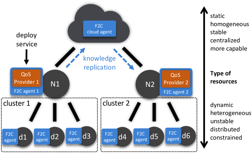
Figure 1: Edge/Fog to Cloud architecture

III System architecture

This section first describes the reference architecture based on a typical fog-to-cloud management system. We then deep dive into the specific modules involved on QoS provisioning, including Service Manager, SLA manager and QoS Provider.

III-A Fog-to-Cloud system architecture

The design and development of the QoS Provider has been performed as part of the fog to cloud architectural platform developed in [2], which by itself is heavily leaning on the fog-to-cloud architectures proposed in Open Fog Consortium standardization body. This architecture considers a hierarchical tree topology of the overall system, where computing devices are connected at different layers according to their compute and storage capabilities and their connectivity. The more static and computationally capable devices are clustered closer to the cloud, while the more dynamic and constrained devices clustered are closer to the bottom of the hierarchy (fog). A simplified representation of this architecture is shown in Fig. 1. In this architecture, every device (or logical cluster) runs a mF2C agent, where depending on the layer in the hierarchy, the agent is expected to play different roles. For instance, in the example with three layers shown in Fig. 1, the intermediate nodes N1 and N2 act as leaders of cluster 1 and 2, respectively. Here, if a service is to be deployed in N1, it will use the resources in cluster 1, and QoS Provider 1 is responsible to provide certain QoS to that service. Although the clustered devices d1, d2 and d3 also have the same F2C agent deployed, QoS provider does play any role there since they are not leaders of the cluster. On the other hand, the cloud agent here only acts as a backup entity for the acquired knowledge in F2C agent 1 to be replicated into other nodes. The generic architecture of every agent is implemented with various functional modules, as shown in Fig. 2. Before starting the description of the QoS provider as part of Service Manager, let us first explain how SLA manager works in the architecture, which is relevant to QoS (other modules are out of scope and can be found in [2]).

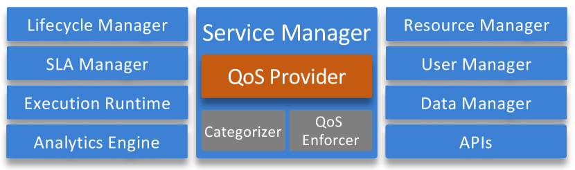
Figure 2: An F2C agent

The SLA Manager implements the creation, storage and evaluation of the agreements. An SLA agreement is a document that declares the QoS guarantees that a service provider offers to a client; as such, the document contains the involved parties, a description of the provided service and a set of guarantee terms. The schema of the mF2C SLA agreements is based on the WS-Agreement specification [13], using a JSON format. This facilitates the management of SLAs by the devices with low computing capabilities that may be present in a clustered area. In particular, the management of SLAs is done by the leader of a cluster area, which is considered the device with higher computing resources. Ideally, each device executes the SLA Management, so it can take over the role of SLA manager in case the leader becomes unaccessible.The guarantee terms in an agreement define the Service Level Objectives (SLOs) that the service provider must fulfill. They are expressed as a constraint on a QoS metric (e.g., service availability of 99.999%). Our architecture considers metrics at the level of the application and the infrastructure. An example of QoS metric at the level of infrastructure is the availability of the devices, while an example at the level of the application is the response time to execute a given operation. For the evaluation, the SLA Management relies on the monitoring metrics provided by the Telemetry and the Distributed Execution Runtime components. The actual value for the metric expressed in the SLO constraint is compared to the threshold, raising an SLA violation when the constraint is not satisfied. The guarantee term, besides the SLO, may define the penalty that applies in case of a violation (e.g. a discount).

1:  N, f = 0

2:  B = N - (N $\cdot$ a)

3:  env = initializeEnvironment(N)

4:  availabilities = initialize(N)

5:  loop

6:       env $\leftarrow$ blockDevices(env, availabilities, B)

7:       service = executeService(env)

8:       f = checkFailure(service)

9:       if f = 1 then

10:             failures = getFailedDevices(env)

11:             failProb = updateFailureProb(env, failures)

12:       end if

13:  end loop

Figure 3: Telemetry based heuristic (TEL) algorithm

III-B Service Manager with QoS Provider

The QoS provider component is part of a Service Manager module which is a component software of mF2C [2]. Apart from the QoS provider, the Service Manager is also composed by the Categorizer and QoS Enforcement. The Categorizer is responsible of registering and categorizing new services into the system, where a service is defined by different parameters such as the application to run, the SLA, the minimum set of devices to run a service, among others. The QoS Enforcement is responsible to add new devices for service execution in runtime in case the system predicts that are not enough resources to fulfill the SLA agreement. When a service is executed for the first time, the Service Manager generates a new QoS model for that specific agent that is going to be executed in a set of specific devices.

The QoS provider module tries to assure that the SLA agreements are fulfilled by blocking or allowing the usage devices based on their availability. Because the QoS provider does not run in runtime (like the QoS enforcer), this decision has to be made in advance, before the execution of a service. For taking this decision, the QoS provider makes use of telemetry data that determines which agents failed in past executions and tries to avoid their usage. The pseudo code of the telemetry based heuristic algorithm (TEL) is shown in Fig. 3. $N$ is the total number of devices and B is the number of devices to block in every iteration. B is determined based on N and a (acceptance ratio). This acceptance ratio is the minimum percentage of required devices for a specific service to run properly. We initialize the environment, which consists of an array of booleans ($d_{1}$, $d_{2}$, …, $d_{n}$) each one representing a device in a cluster where an instance of the algorithm is running, and the availabilities by specifying the number of agents. Then, we enter in the loop that is run for every service execution. Inside the loop, we call a function to block devices specifying the environment, the availabilities and the number of devices to block. After the service is executed specifying which devices can be used, the algorithm checks whether the service was disrupted or not from telemetry data provided by Analytics Engine (see Fig.2). In case of disruption (f = 1), we check which devices were not available during the execution and we update the new availabilities of each device.

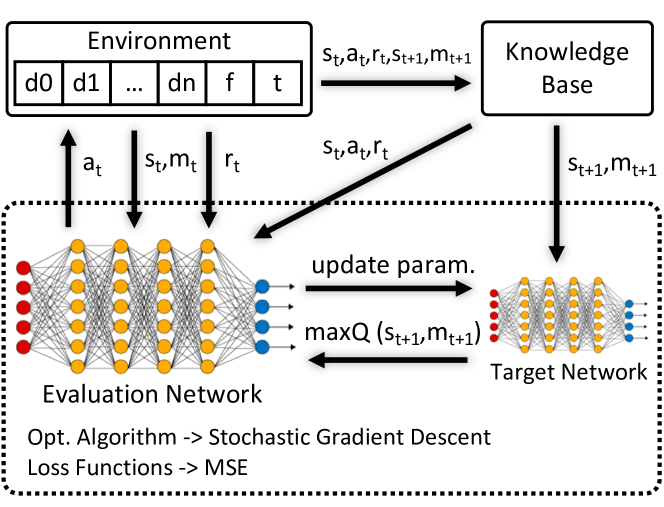
Figure 4: Deep Reinforcement Learning model

IV Integrating Deep Reinforcement Learning (DRL) into the QoS provider

In reinforcement learning models, an agent takes some actions in an environment based on observations, where later those actions are rewarded back to the agent. The objective is to maximize the cumulative reward through performing actions, in some cases prioritizing short term rewards or in other cases looking forward to future long term rewards. Fig. 4 represents our model design. The environment consists of an array of booleans ($d_{1}$, $d_{2}$, …, $d_{n}$), each one representing a device in a cluster (see Fig. 1), plus an specific boolean $f$, used to indicate that the service execution failed, plus an integer $t$ to determine the time step. Each boolean represents whether a specific device $d_{x}$ is blocked for allocation (value 1) or allowed (value 0). Therefore, considering $N$ the total number of devices, the length of the environment is equal to $N+2$. From this environment, which will be modified into a new state on every iteration, a new input is generated for the evaluation network. Because in every iteration $t$, a new state $s_{t}$ from the environment is generated, a new reward $r_{t}$ is calculated based on the previous action and the weights of the network updated. The number of outputs is determined based on the number of devices to allow or block for allocation. Since the individual decision of blocking and allowing a certain device are probabilistically independent, two actions are possible for every device, plus the action of not performing any action at all. Therefore, the output length of the model is equal to $2N+1$. From the output values, the algorithm selects one action $a_{t}$ based also on a mask $m_{t}$. The mask has the same length as the output and is used to limit the actions the agent can take for an specific environment. The next example, when $N=2$, shows the simplified procedure of the algorithm:

$$environment(s_{t}) =[1,0,0,2]$$ (1a)

$$mask(s_{t}) =[1,0,0,1,1]$$ (1b)

$$output(s_{t}) =[2.11,3.02,1.55,0.053,0.12]$$ (1c)

$$action(s_{t}) =0$$ (1d)

$$environment(s_{t+1}) =[0,0,0,3]$$ (1e)

$$reward(s_{t+1}) =r$$ (1f)

In this example, the environment length is 4, where the two first positions indicate whether devices 1 and 2, respectively, are allowed (0) or blocked (1), the third position indicates whether the service is disrupted or not, and the last position indicates the time step. Then, a mask at the state $s_{t}$ is generated, setting array elements to 0 when an action cannot be performed; and to 1, otherwise. In this specific example, considering the mask has $K=5$ elements and based on the environment($s_{t}$), the element $k=0$ determines if the first device from the environment can be switched to allowed. Because in the environment that device was blocked, for this iteration we set the element $k=0$ to 1 to indicate that the device can be allowed. However, because it was already blocked, the element $k=1$ of the mask is set to 0, to not allow the algorithm to block that device again. The same procedure applies for the second device, where the elements $k=2$ is set to 0 and $k=3$ is set to 1, to specify to the algorithm that it can block that device but not allowing it again. This procedure is necessary to maintain each allow and block probabilities independent for every device providing more knowledge to the model for the decision process. In case the optimum decision is to not perform any action on a specific state, the last element of the mask is used for that purpose, being always set to 1. Then, based on the mask($s_{t}$), an action is taken at instance $s_{t}$, according to the values from the output array. The action is equal to the position of the array with the maximum value that the mask allows to use. In this case, the maximum value from the output that the mask allows to use is $2.11$, so the action is equal to that position in the array, i.e. 0. This action modifies the environment for the next time step, by switching from 1 to 0 the first element of the environment. It is to be noted that the last element of the environment is just the time step counter; in this case it indicates that is the 4th iteration of the algorithm. At that point a reward($s_{t+1}$) is calculated taking into account the current state of the environment and the model updates the network values for the next iteration.

The algorithm consists of a function $Q$ that calculates the quality of actions in different combinations of states. So, at each state $s_{t}$, the agent chooses an action $a_{t}$, observes a reward $r_{t}$ and updates into an new state $s_{s+1}$. This process updates iteratively the function $Q$ following the next equation:

$$Q_{t+1}(s_{t},a_{t})=Q_{t}(s_{t},a_{t})+\alpha[R(s_{t},a_{t})+\gamma\cdot\max Q(s_{t+1},a_{t+1})]$$ (2)

, where $Q_{t+1}(s_{t},a_{t})$ is the updated value for next iteration and $Q_{t}(s_{t},a_{t})$ is the old Q value. The $\alpha$ value is the learning rate ($0<\alpha\leq 1$) which determines the weight between the new information and the previous one. The closer $\alpha$ value is to 0, the less new information the agent learns, while the closer to 1, the more new information the agent leans. $R(s_{t},a_{t})$ is the reward observed after performing an action $a_{t}$ in state $s_{t}$. $\gamma$ ($0<\gamma\leq 1$) is the discount factor which determines the importance of future rewards in comparison with immediate rewards. A $\gamma$ close to 0 makes future rewards worth less than immediate values, while a value close to 1 makes future rewards worth as much as immediate rewards. The $\max Q(s_{t+1},a_{t+1})$ value is the maximum estimated future reward given the new state $s+1$ and the possible actions for that specific state $a_{t+1}$. To be observed, that this value is calculated from the target network which is a copy of the evaluation network, but which parameters are only updated at certain frequency and not in every step as for the evaluation network. This is done to improve convergence of training and stability to the model. Both neural networks will be updated by stochastic gradient descent and will use Mean Square Error as the loss function.

1:  N, action = -1, f = 0, t = 0, r = 0

2:  env = initializeEnvironment(N, f, t)

3:  nextEnv = initialize(N, f, t + 1)

4:  mask = generateMask(env)

5:  loop

6:       service = executeService(env)

7:       nextEnv $\leftarrow$ f = checkFailure(service)

8:       reward = computeReward(nextEnv)

9:       nextMask = generateMask(nextEnv)

10:       addExp(env, nextEnv, action, reward, nextMask)

11:       trainNetwork()

12:       env = nextEnv

13:       mask = generateMask(env)

14:       action = getAction(env, mask)

15:       nextEnv = modifyEnvironment(env, action)

16:  end loop

Figure 5: Deep Reinforcement Learning (DRL) algorithm

A pseudo algorithm is shown in Fig. 5. Before starting to iterate, the environments, env and nextEnv, are initialized by specifying the number of devices (N) in the cluster. Also, an initial mask is generated from the initial environment, following the procedure previously mentioned. From this point, the algorithm enters in a loop where every iteration is an execution of the specific service. For every iteration, the first step is to check if the service failed in the previous iteration; if so, the nextEnv is modified by switching the $f$ value to 1. Then, a reward is calculated based on nextEnv, where the status of each device (blocked or allowed) is checked, while considering if the service failed or not, and points are given according to that. The total reward is the summation of points per device having 4 different cases: 1) $+10$ points, if a device was allowed and service did not fail, 2) $-10$ points, if a device was allowed and service failed, 3) $0$ points, if a device was blocked and service did not fail and 4) $-10$ points, if a device was blocked and the service failed. With this reward function, we are positively rewarding the cases where more devices are allowed and no service failures occur. On the contrary, we are penalizing the cases where there is a service failure without differentiating whether a certain device was allowed or blocked. Finally, we are not rewarding at all the cases where devices are blocked and no service failure ocurred. While this last case is positive, the objective is to maximize the number of used devices, therefore, by not rewarding we are pushing the model to try to allow devices as long as they do not cause service failures. Then, a new mask nextMask based on the nextEnv is created and the model adds a new experience to the knowledge base, where the env, the nextEnv, the action, the reward and the nextMask are specified (see also Fig. 4). The next step is training the evaluation network which consists on calculating the function $Q$, previously explained, per a batch of experiences, where the batch_size is a parameter value. This training will only occur after the number of experiences is greater than an initial value start_size. The maximum number of experiences that the model can store in the knowledge base is determined by a memory_capacity value. When a new experience is created and the memory is full, a randomly old experience is removed to let the new experience be added. This is done to limit the amount of used memory and to remove old knowledge that is no longer needed. Then, once the network acquired the knowledge, the nextEnv is stored as env and a new mask is generated. Both env and mask are used to get an action according to the maximum value of the output the evaluation network. Once, the action is determined, the nextEnv is recreated for the next iteration. The next iteration will occur, before the next service execution occurs, when the model is asked again for a new decision.

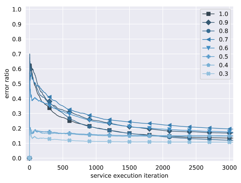
(a) DRL - 5 devices

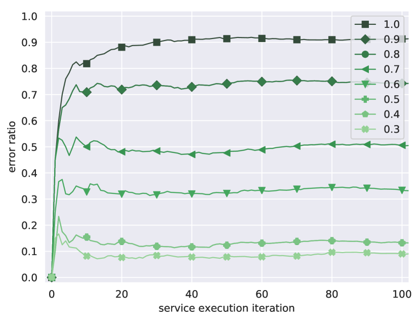
(b) TEL - 5 devices

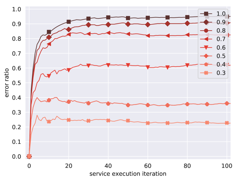
(c) RND - 5 devices

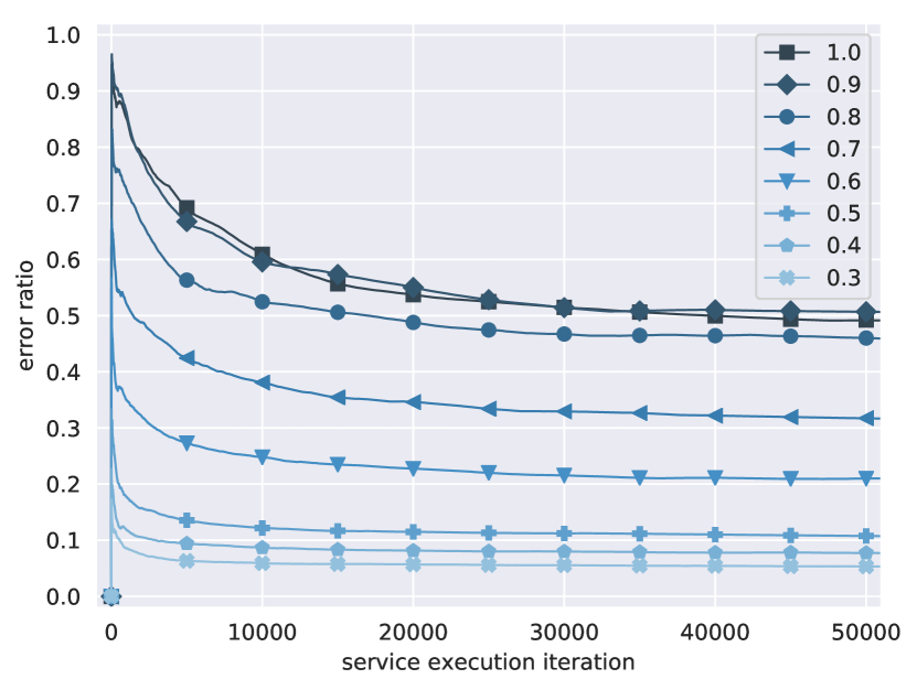
(d) DRL - 10 devices

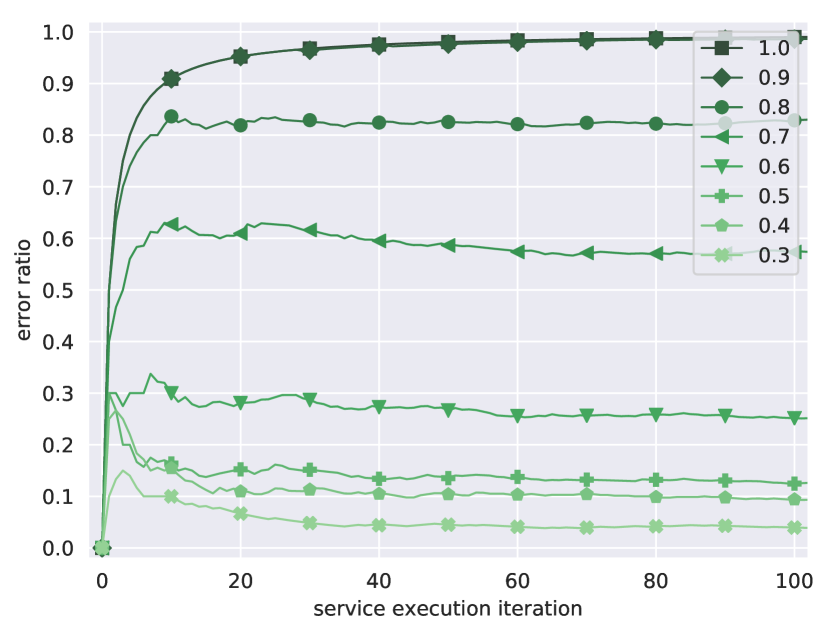
(e) TEL - 10 devices

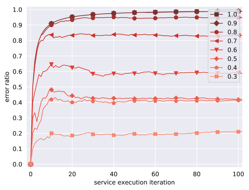
(f) RND - 10 devices

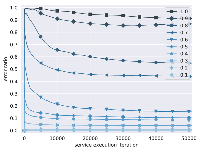
(g) DRL - 15 devices

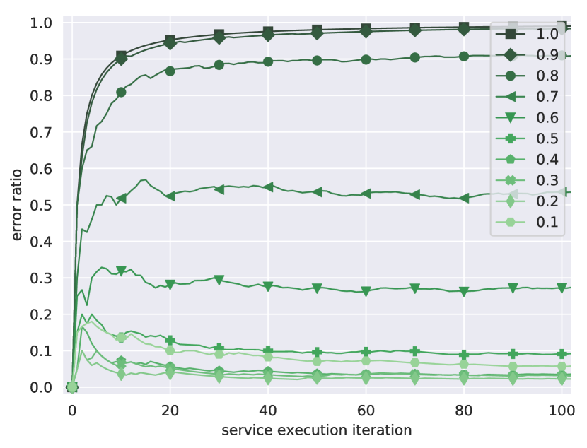
(h) TEL - 15 devices

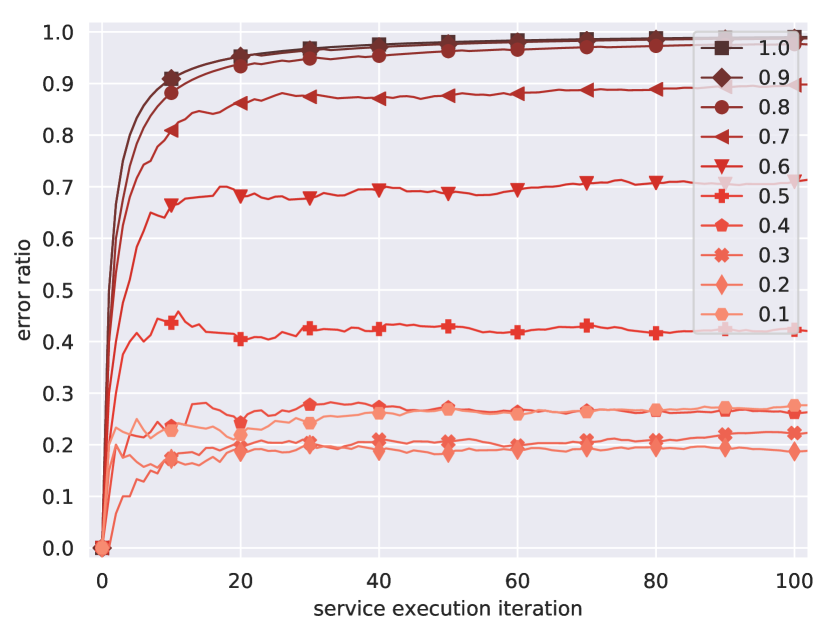
(i) RND - 15 devices

Figure 6: Error ratio running average per service executions

V Performance Evaluation

The software development described in this paper is open source and publicly available in [2]. For the implementation of the DRL algorithm we have used Eclipse Deeplearning4j library, with the next parameters for the model: memory_capacity is 100000, batch_size and start_size are both 10, the discount_factor is 0.1 and the num_hidden_layers is 150. All tests have been performed in a Intel Core i7-6700 CPU at 3.4GHz with 32 GB of RAM. For the sake of comparison, we also implemented a random selection (RND) algorithm based, where the devices that are block are randomly chosen. For all evaluations, instead of executing real services, we just emulate the volatility of devices following a uniform distributed function of the probability that the device fails, with the same initial seeds for all three algorithms. To determine whether a service has been disrupted or not, we use the acceptance_ratio. Therefore a service is disrupted when the ratio of volatile devices divided by the total number of devices used for the service execution is bigger than the acceptance ratio. For instance, let us consider a cluster of 5 devices with an acceptance_ratio = 0.5 and all 5 devices are used for launching a service. If during the service execution 3 or more devices are volatile, then the service will be disrupted.

Fig. 6 shows the disruption ratio running average per service execution when clustering 5, 10 and 15 devices, and Table I shows the total average service disruption ratio for 100k service executions. We evaluated the algorithms in all cases for acceptance ratios from 0.3 to 1.0. For the DRL algorithm, we show the running average for 3000 service executions when clustering 5 devices and 50k service executions when clustering 10 and 15 devices. For the TEL and RND cases, we only show the first 100 executions, then the values become constant, however, the total average can be found in Table I. When comparing all three algorithms when clustering 5 devices (see Fig 6(a), 6(b) and 6(c)), we can see how DRL performs much better than TEL or RND for any acceptance ratio, even during the first service executions. The reason is related to the number of possible actions that DRL can take. Because DRL can only perform one action per service execution, when the number of possible actions (proportional to the number of devices) is low, the algorithm has more chances to predict the device that will fail. Instead, although TEL can block multiple devices per service execution, this blocking is only based on probability of failure. In RND case, the results are even worse than in TEL, because the blocking decision is randomly taken. When running the algorithms for 10 devices (see Fig. 6(d), 6(e) and 6(f)) DRL still performs better in long term compared to the other two, but here we can see how this difference is less significant or negligible when the acceptance ratio is lower than 0.6 when compared to TEL (also in Table I). This is because, the lower acceptance ratio the lower number of devices need to blocked, and then reducing the probability for the TEL to miss a device that will potential fail. The last case, when comparing the results for 15 devices, we can see how with acceptance ratio of 0.7 or lower, there is no benefit of using DRL over TEL, and only in long term (with more than 10k executions) in some cases DRL overperforms TEL. These results show how DRL solution performs much better with a low number of devices, due to the lower amount for actions from where the algorithm has to choose. For a high number of devices there is no benefit of using DRL instead of traditional TEL algorithms. We finally measured the average execution times over 100 repetitions after 10 warmups for all algorithms. With 5 devices in the cluster DRL takes $333.797\pm 2.965$ ms, TEL $0.153\pm 0.010$ ms and RND $0.150\pm 0.001$ ms. For 10 devices DRL takes $336.241\pm 34.058$ ms, TEL $0.328\pm 0.009$ ms and RND $0.312\pm 0.010$ ms. For 15 devices DRL takes $394.507\pm 24.173$ ms, TEL $0.834\pm 0.045$ ms and RND $0.523\pm 0.029$ ms. We can see that DRL is much slower compared to TEL, but the amount of time is still negligible.

TABLE I: Total average error ratio for 100k service executions

	5 devices			10 devices			15 devices
	DRL	TEL	RND	DRL	TEL	RND	DRL	TEL	RND
1.0	0.08	0.92	0.96	0.47	$0.\overline{99}$	$0.\overline{99}$	0.90	$0.\overline{99}$	$0.\overline{99}$
0.9	0.11	0.75	0.91	0.52	0.99	$0.\overline{99}$	0.87	0.99	$0.\overline{99}$
0.8	0.08	0.75	0.91	0.45	0.84	0.95	0.53	0.90	0.99
0.7	0.15	0.52	0.82	0.31	0.57	0.85	0.41	0.51	0.89
0.6	0.10	0.33	0.63	0.20	0.23	0.60	0.13	0.22	0.72
0.5	0.15	0.12	0.38	0.10	0.10	0.43	0.10	0.05	0.43
0.4	0.13	0.12	0.38	0.07	0.08	0.43	0.08	0.02	0.27
0.3	0.10	0.08	0.25	0.05	0.02	0.20	0.04	0.01	0.22

VI Conclusion

We proposed a QoS provider mechanism, as an integral component of a real world fog-to-cloud system, to work in dynamic edge computing scenarios based on reinforcement learning. Specifically, we developed a deep Q-learning algorithm which is particularly well suited in dynamic and adaptive environments where the decision process needs to be frequently updated. We compared our solution with a telemetry based heuristic algorithm, showing how reinforcement learning is able to overperform when the number of devices to manage is low. As future work, we will extend our algorithm to allow multiple actions per service execution, expecting to improve the results when increasing the number of managed devices.

References

- [1] F. Faniyi and R. Bahsoon, “A Systematic Review of Service Level Management in the Cloud,” ACM Computing Surveys, 2015.
- [2] H2020, “mF2C: Towards an Open, Secure, Decentralized and Coordinated Fog-to-Cloud Management Ecosystem.” [Online]. Available: http://www.mf2c-project.eu
- [3] O. Consortium, “OpenFog Consortium,” 2017. [Online]. Available: https://www.openfogconsortium.org/
- [4] T. Y. Kan, Y. Chiang, and H. Y. Wei, “Task offloading and resource allocation in mobile-edge computing system,” 2018 27th Wireless and Optical Communication Conference, WOCC 2018, pp. 1–4, 2018.
- [5] Y. Song, S. S. Yau, R. Yu, X. Zhang, and G. Xue, “An Approach to QoS-based Task Distribution in Edge Computing Networks for IoT Applications,” Proceedings - 2017 IEEE 1st International Conference on Edge Computing, EDGE 2017, pp. 32–39, 2017.
- [6] L. Huang, G. Li, J. Wu, L. Li, J. Li, and R. Morello, “Software-defined QoS provisioning for fog computing advanced wireless sensor networks,” Proceedings of IEEE Sensors, pp. 1–3, 2017.
- [7] D. H. Li and D. Levy, “A reinforcement learning based self-optimizing QoS controller framework for distributed services,” 2010 Chinese Control and Decision Conference, CCDC 2010, pp. 2917–2922, 2010.
- [8] H. Khelifi, S. Luo, B. Nour, A. Sellami, H. Moungla, S. H. Ahmed, and M. Guizani, “Bringing Deep Learning at the Edge of Information-Centric Internet of Things,” IEEE Communications Letters, 2019.
- [9] J. Wang, L. Zhao, J. Liu, and N. Kato, “Smart Resource Allocation for Mobile Edge Computing: A Deep Reinforcement Learning Approach,” IEEE Transactions on Emerging Topics in Computing, vol. PP, no. c, pp. 1–1, 2019.
- [10] M. Abundo, V. Di Valerio La Sapienza, V. Cardellini, and F. L. Presti, “QoS-aware bidding strategies for VM spot instances: A reinforcement learning approach applied to periodic long running jobs,” Proceedings of the 2015 IFIP/IEEE International Symposium on Integrated Network Management, IM 2015, pp. 53–61, 2015.
- [11] S. C. Lin, I. F. Akyildiz, P. Wang, and M. Luo, “QoS-aware adaptive routing in multi-layer hierarchical software defined networks: A reinforcement learning approach,” Proceedings - 2016 IEEE International Conference on Services Computing, SCC 2016, pp. 25–33, 2016.
- [12] Y. Wei, L. Pan, S. Liu, L. Wu, and X. Meng, “DRL-Scheduling: An intelligent QoS-Aware job scheduling framework for applications in clouds,” IEEE Access, vol. 6, pp. 55 112–55 125, 2018.
- [13] A. Andrieux, K. Czajkowski, A. Dan, and K. Keahey, “Web services agreement specification (WS-Agreement),” Tech. Rep. [Online]. Available: https://www.ggf.org/Public_Comment_Docs/Documents/Oct-2006/WS-AgreementSpecificationDraftFinal_sp_tn_jpver_v2.pdf