Evolution of Magnetic Helicity in Solar Cycle 24

Abstract

We propose a novel approach to reconstruct the surface magnetic helicity density on the Sun or sun-like stars. The magnetic vector potential is determined via decomposition of vector magnetic field measurements into toroidal and poloidal components. The method is verified using data from a non-axisymmetric dynamo model. We apply the method to vector field synoptic maps from Helioseismic and Magnetic Imager (HMI) on board of Solar Dynamics Observatory (SDO) to study evolution of the magnetic helicity density during solar cycle 24. It is found that the mean helicity density of the non-axisymmetric magnetic field of the Sun evolves in a way which is similar to that reported for the current helicity density of the solar active regions. It has predominantly the negative sign in the northern hemisphere, and it is positive in the southern hemisphere. Also, the hemispheric helicity rule for the non-axisymmetric magnetic field showed the sign inversion at the end of cycle 24. Evolution of magnetic helicity density of large-scale axisymmetric magnetic field is different from that expected in dynamo theory. On one hand, the mean large- and small-scale components of magnetic helicity density display the hemispheric helicity rule of opposite sign at the beginning of cycle 24. However, later in the cycle, the two helicities exhibit the same sign in contrast with the theoretical expectations.

1 Introduction

Magnetic helicity is an integral measure of topological properties of the magnetic field in closed volume $\rm V$:

$$H_{M}=\int\mathbf{A}\cdot\mathbf{B}d\mathrm{V},$$ (1)

where $\mathbf{A}$ is the magnetic vector potential, $\mathbf{B}=\boldsymbol{\nabla}\times\mathbf{A}$, and the $\mathbf{B}$ is confined to the volume $\mathrm{V}$. Locally, it can be characterized by a number of parameters such as linkage, twist and writhe of the field lines (Berger & Hornig, 2018). In astrophysical dynamos, magnetic helicity is commonly accounted as a nonlinear constraint of turbulent generation of large-scale magnetic field (Pouquet et al., 1975; Kleeorin & Ruzmaikin, 1982; Brandenburg & Subramanian, 2005). Computation of magnetic helicity on the Sun requires knowledge of vector magnetic field in a 3D region, but observations are usually taken in a shallow layer of the solar atmosphere (typically, in the photosphere). Thus, early studies turned to calculation of so-called helicity proxies, such as, for example, vertical components of current helicity density $J_{z}\cdot B_{z}$ or $\alpha=J_{z}/B_{z}$ (a measure of magnetic twist). Seehafer (1990) and Pevtsov et al. (1995) found that the current helicity density and twist in solar active regions follow $\it{the~{}hemispheric~{}helicity~{}rule}$ with predominantly negative values in the northern hemisphere and positive values in the southern hemisphere. The hemispheric preference for the helicity sign was later confirmed by several researchers (e.g., Longcope et al., 1998; Bao & Zhang, 1998; Hagino & Sakurai, 2005). Choudhuri et al. (2004) proposed that due to interaction of the large-scale toroidal field from a previous solar cycle and the poloidal field of a new cycle, the hemispheric helicity could reverse sign at the beginning of each cycle. Hagino & Sakurai (2005) reported the presence of such sign reversal in the Okayama Observatory Solar Telescope (OAO) and the Mitaka Solar Flare Telescope (SFT) observations. Pevtsov et al. (2008) examined the periods of sign reversals observed by different instruments and found no agreement among the datasets during these periods. They concluded that at least some reversals could be due to statistical nature of the hemispheric helicity rule. Later, Zhang et al. (2010) showed that hemispheric helicity rule of the solar active regions evolve with time and found its reversals at the beginning of Solar Cycles 22 and 23. Sokoloff et al. (2013) found inversions of the current helicity density in active regions at the beginning and at the end of the solar cycle 23. These early findings are based on vector magnetograms of active regions only. Systematic full disk observations of vector magnetic field became available in 2009 from Vector Spectromagnetograph (VSM) on Synoptic Optical Long-term Investigations of the Sun (SOLIS) platform (Balasubramaniam & Pevtsov, 2011) and in 2010 from Helioseismic and Magnetic Imager (HMI, Scherrer et al., 2012) on board Solar Dynamics Observatory (SDO, Pesnell et al., 2012). Prior to these observations, calculations of current helicity relied on vector magnetic field reconstructed from rotational modulation of the observed longitudinal (line-of-sight) field (Pevtsov & Latushko, 2000). Later studies demonstrated that the sign of helicity of large-scale magnetic fields is opposite to the sign of helicity of active regions (Pipin & Pevtsov, 2014; Brandenburg et al., 2017). The large-scale helicity was also found to evolve during solar cycles similarly to helicity of active regions.

The solar dynamo theory predicts bi-helical properties of magnetic fields (Blackman & Brandenburg, 2002; Brandenburg & Subramanian, 2005). In this theory the sign of magnetic helicity density of large-scale field should correspond to the sign of the $\alpha$-effect, while sign of magnetic helicity density of the small-scale field would result from the magnetic helicity conservation, and thus, it would be opposite to large-scale helicity. In the framework of this model, small-scale magnetic field corresponds to active regions and the large-scale stands for the global axisymmetric components of the solar magnetic activity. The bi-helical properties were studied recently by Brandenburg et al. (2017) and Singh et al. (2018) using two-scale approximation and the vector magnetic field measurements from SDO/HMI and SOLIS. The results from two different instruments appear to be inconclusive in respect to bi-helical nature of solar magnetic field.

Other predictions of mean-field dynamo models include the existence of polar and equatorial branches in the time-latitude diagram of magnetic helicity evolution. According to Pipin et al. (2013), those branches represent the transport of magnetic helicity flux to the polar regions, both on large and small scales. In this paper we present the first observational evidence of polar branches of the large-scale magnetic helicity in solar cycle 24. Section 2 describes our method of calculation of magnetic helicity. Section 3 verifies the proposed methodology using synthetic data from mean-field dynamo model calculations. Section 4 presents the derivation of magnetic helicity using observed magnetic fields, and Section 5 discusses our findings.

2 The method

To determine the magnetic helicity density, we employ a decomposition of the vector magnetic field into toroidal and poloidal components using scalar potentials $S$ and $T$ (Krause & Rädler, 1980; Berger & Hornig, 2018):

$$\mathbf{B} = \boldsymbol{\nabla}\times\left(\hat{\mathbf{r}}T\right)+\boldsymbol{\nabla}\times\boldsymbol{\nabla}\times\left(\hat{\mathbf{r}}S\right)=$$ (2)

$$= -\frac{\hat{r}}{r}\Delta_{\Omega}S+\hat{\theta}\left(\frac{1}{\sin\theta}\frac{\partial T}{\partial\phi}-\frac{\sin\theta}{r}\frac{\partial F_{S}}{\partial\mu}\right)+\hat{\phi}\left(\sin\theta\frac{\partial T}{\partial\mu}+\frac{1}{r\sin\theta}\frac{\partial F_{S}}{\partial\phi}\right)$$

where ${\displaystyle\Delta_{\Omega}=\frac{\partial}{\partial\mu}\sin^{2}\theta\frac{\partial}{\partial\mu}+\frac{1}{\sin^{2}\theta}\frac{\partial^{2}}{\partial\phi^{2}}}$, $\mu=\cos\theta$ and $\theta$ is the polar angle, and $F_{S}=\partial\left(rS\right)/\partial r$. Three components of vector magnetic field (radial $r$, meridional $\theta$, and zonal $\phi$, see, Virtanen et al., 2019) are then represented by three independent variables, $S$ , $T$, and $F_{S}$:

$$B_{r} = -\frac{1}{r}\Delta_{\Omega}S,$$ (3)

$$B_{\theta} = \frac{1}{\sin\theta}\frac{\partial T}{\partial\phi}-\frac{\sin\theta}{r}\frac{\partial F_{S}}{\partial\mu},$$ (4)

$$B_{\phi} = \sin\theta\frac{\partial T}{\partial\mu}+\frac{1}{r\sin\theta}\frac{\partial F_{S}}{\partial\phi}$$ (5)

To determine a unique solution of Equations 3–5 we apply the following gauge (see, e.g., Krause & Rädler 1980):

$$\int_{0}^{2\pi}\int_{-1}^{1}Sd\mu d\phi=\int_{0}^{2\pi}\int_{-1}^{1}Td\mu d\phi=\int_{0}^{2\pi}\int_{-1}^{1}F_{S}d\mu d\phi=0.$$ (6)

Note, that in the case of potential magnetic field $T=0$, and $F_{S}$ is determined by $S$. Therefore, the system of Equations 3–5 represents a least-squares problem. Hereafter we consider the general case of nonpotential magnetic fields on the solar surface. Eqs.(3), (4) and (5) can be transformed in:

$$-\frac{1}{r}\Delta_{\Omega}S = B_{r}$$ (7)

$$\Delta_{\Omega}T = \frac{\partial}{\partial\mu}\sin\theta B_{\phi}+\frac{1}{\sin\theta}\frac{\partial B_{\theta}}{\partial\phi},$$ (8)

$$\frac{1}{r}\Delta_{\Omega}F_{S} = \frac{1}{\sin\theta}\frac{\partial B_{\phi}}{\partial\phi}-\frac{\partial}{\partial\mu}\sin\theta B_{\theta}$$ (9)

Reconstruction and differentiating is done in the spectral spherical harmonic space using the SHTools (Wieczorek & Meschede, 2018). After finding solutions for $S$, $T$ and $F_{S}$ we can determine components of vector potential $\mathbf{A}$,

$$\mathbf{A} = \hat{\mathbf{r}}T+\boldsymbol{\nabla}\times\left(\hat{\mathbf{r}}S\right)=$$ (10)

$$= \hat{\mathbf{r}}T+\frac{\hat{\theta}}{\sin\theta}\frac{\partial S}{\partial\phi}+\hat{\phi}\frac{\sin\theta}{r}\frac{\partial S}{\partial\mu}.$$

Below we demonstrate the method using output of a dynamo model, where we have complete information about the distribution of vector magnetic field, its vector potential and magnetic helicity density.

3 Dynamo Model Benchmark

We use results of the non-axisymmetric $\alpha^{2}\Omega$ dynamo model developed recently by Pipin & Kosovichev (2018). The model simulates the solar-type dynamo, in which the surface magnetic activity is governed by the dynamo-generated axisymmetric toroidal magnetic field. The dynamo parameters of the model are below threshold of the dynamo instability of large-scale non-axisymmetric magnetic fields. This resembles the situation for solar-type dynamos (Raedler, 1986). In order to mimic emergence of solar active regions, we take into account the Parker’s magnetic buoyancy instability, which produces bipolar regions from the toroidal magnetic field at random latitudes and random moment of time under the condition that the magnetic field strength exceeds a critical threshold. The reader can find a detailed description of the model and the code in Pipin & Kosovichev (2018) and Pipin (2018).

Figure 1 shows snapshots of the magnetic field components, as well as the magnetic and current helicity densities. The snapshots are taken during the maximum of the dynamo cycle. The magnetic helicity has predominantly positive sign in the northern hemisphere and the negative sign in the southern hemisphere. In this case, the hemispheric helicity rule of the large-scale magnetic field follows from the dynamo theory which predicts that the sign of the magnetic helicity of the large-scale field corresponds to the sign of the $\alpha$-effect in a given hemisphere (Blackman & Brandenburg, 2003; Singh et al., 2018).

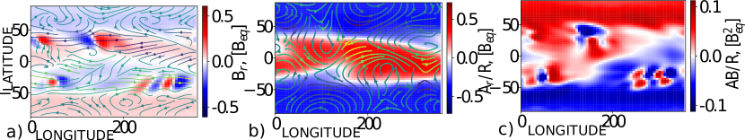
Figure 1: a) Snapshot of the radial magnetic field distribution (color image), streamlines show the horizontal (toroidal and poloidal) magnetic field; b) snapshot for the magnetic helicity density; c) the radial component of the current helicity density $H_{C}=B_{r}\left(\boldsymbol{\nabla}\times\mathbf{B}\right)_{r}$.

4 Magnetic Helicity Density Derived From Observations

4.1 Observational Data

We apply the formalism described in Section 2 to a set of intermediate resolution (360 by 720 pixels) vector magnetic fields synoptic maps from HMI/SDO. The dataset includes 116 Carrington rotations (CR) from CR2097 (May 2010) to CR2214 (March 2019). The HMI synoptic maps are calculated in Carrington longitude (degrees) – sine (latitude) coordinate grid. The pixel size is 0.5 degree in longitude and 1/180 in sine latitude. Method for producing the HMI synoptic maps is described in details by Liu et al. (2017). For these data, the 180 degree ambiguity in the horizontal field direction was resolved by the HMI team using a combination of a minimum energy criterium (for pixels with stronger fields) and random disambiguation (for weak field pixels). Additional details about the HMI data reduction and the disambiguation procedure can be found in the above cited paper.

Liu et al. (2017) found that with the chosen combination of disambiguation methods the noise level of the vector magnetic field in the synoptic charts varies from $\pm 10$G during the solar maximum to $\pm 20$G during the solar minimum.

4.2 Results

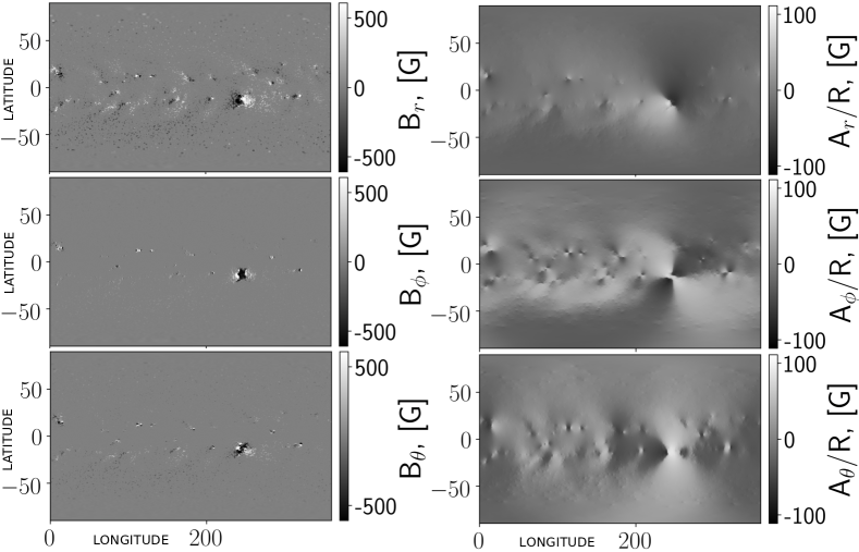
Figure 2: Synoptic maps of the vector magnetic field and the reconstructed potential from SDO/HMI for CR 2156.

As the first example, we consider results of reconstruction of the vector potential for the synoptic maps of CR2156. This Carrington rotation is characterized by strong active region NOAA AR 12192 that emerged in the southern hemisphere. Figure 2 shows the synoptic maps of the vector magnetic field and the reconstructed potentials $\mathrm{S}$, $\mathrm{A_{r}=rT}$. Distribution of the vector potential reveals a large-scale non-axisymmetric pattern associated with this active region. Interesting that the vector-potential components show inverse sign relative to the corresponding magnetic field components in the core of the active region. This results in predominantly negative magnetic helicity in AR 12192, which is shown in Figure 3. We notice that the east part of the southern hemisphere shows the background magnetic helicity of the positive sign which corresponds to the basic hemispheric helicity of the active regions (Pevtsov et al., 2014). The large area of the negative magnetic helicity density around NOAA AR 12192 resembles the situation demonstrated in our dynamo model. Thus, it can be speculated that the origin of this active region is related to large-scale magnetic field located in a shallow subsurface layer.

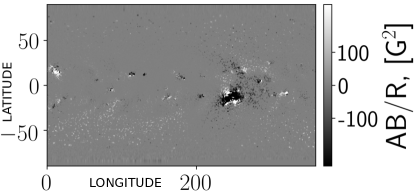
Figure 3: Distribution of the magnetic helicity density $\mathbf{A}\cdot\mathbf{B}$ for CR 2156.

Solving Equations 3–5 for each Carrington rotation from CR2097 to CR2214 we derived the distributions of the vector potential and magnetic helicity density for solar cycle 24. The large-scale distributions of magnetic field and helicity density are obtained by means of the azimuthal averaging of the synoptic maps for each Carrington rotation. To represent the mean signal, where we filtered out the time variations with period less than 2 year. Also, we employ the Gaussian smoothing with a FWHM equal 5 pixels in latitude and 10 CR time. Figure 4 shows the time-latitude diagrams for the axisymmetric components of magnetic field and vector potential. The time-latitude diagrams of the magnetic field evolution are in agreement with Vidotto et al. (2018). The reconstructed potentials disagree with results of Pipin & Pevtsov (2014), who used profiles of $\bar{B}_{r}$ from different longitudinal distances from the central meridian to reconstruct $\bar{B}_{\phi}$ and $\bar{A}_{r}$. Also, the obtained $\bar{B}_{\phi}$ disagrees with our results at the polar-ward side of the sunspot activity zone, where the large-scale toroidal magnetic field is present. The sign of this field is opposite to the sign of toroidal field in the solar active regions. Such bi-modal structure of the axisymmetric toroidal magnetic field affects the distribution of $\bar{A}_{r}$. The sign of the polar-ward side of the axisymmetric toroidal magnetic field can hardly be explained by surface effect of the differential rotation acting on the meridional component of the axisymmetric magnetic field. From Figure 4 it is clear that the direction of the meridional component is opposite to the one which might produce the polar-side toroidal magnetic field. Also, in our case, the evolution of $\bar{A}_{\phi}$ differs from results of Stenflo & Guedel (1988); Blackman & Brandenburg (2003) and Pipin & Pevtsov (2014) as well, where they found symmetric $\bar{A}_{\phi}$ profiles relative to the equator. The difference is likely due to the rather asymmetric development of Cycle 24 in the northern and southern hemispheres.

Figure 5a shows the time-latitude diagrams of the magnetic helicity density of the large-scale field, $\bar{\mathbf{A}}\cdot\bar{\mathbf{B}}$. The magnetic helicity of the large-scale field is positive in the high-latitude zone of the northern hemisphere at the beginning of Cycle 24, and it changes the sign to negative after the polar field reversal. A similar situation is observed in the southern hemisphere. Figure 5b shows the time-averaged hemispheric helicity sign rule together with uncertainty bars. The uncertainties are estimated by using differences of the original and smoothed signals. It is seen that in average over the cycle 24 the large scale magnetic field shows the same hemispheric sign as the “small-scale” magnetic field. However if we would restrict the averaging period to the first half of the cycle 24, i.e., by CR2097–2156 we get, in general, the positive magnetic helicity density in the northern hemisphere and negative in the southern one (except the low latitudes). Therefore at this period of time the bi-helical property can be confirmed with some reservations. This agrees with the two-scale analysis of Brandenburg et al. (2017) as well as with results of Pipin & Pevtsov (2014) (cf., Fig9a there). Also, Figures 5c and d support this conclusion.

Figure 5c shows evolution of “small-scale” magnetic helicity density, i.e., $\mathbf{\overline{a\cdot\mathbf{b}}}=\overline{\mathbf{{A}\cdot\mathbf{{B}}}}-\mathbf{\overline{A}\cdot\mathbf{\overline{B}}}$. The definition of small-scale helicity, $\mathbf{\overline{a\cdot\mathbf{b}}}$, includes magnetic fields from all range of scales except the axisymmetric magnetic field. A more accurate analysis of the magnetic helicity distribution over the scales can be done by using the two-scale analysis introduced by Brandenburg et al. (2017). Averaged over the cycle $\mathbf{\overline{a\cdot\mathbf{b}}}$, shows the hemispheric helicity rule for the solar active regions. It shows the large uncertainty bars which are mostly caused by fluctuations in magnetic flux emergence. It is also can be seen that for the first half of the cycle 24 the $\mathbf{\overline{a\cdot\mathbf{b}}}$ holds the hemispheric helicity rule. The violation of the rule in the time-averaged signal is likely caused by the magnetic activity in the Southern hemisphere during 2014–2015 years. In particular, the active region NOAA 12192 strongly violates the hemispheric helicity rule as we see in Figure 3. In the end of our observational period, the $\mathbf{\overline{a\cdot\mathbf{b}}}$ shows inversion of helicity sign in the low latitudes. This agrees with the results for the current helicity density evolution in cycle 23 (e.g., Zhang et al., 2010).

We find that the standard error for $\bar{\mathbf{A}}\cdot\bar{\mathbf{B}}$/R is less than 1 G² and has maximum at the sunspot formation latitudes. Similarly, the standard error of $\mathbf{\overline{a\cdot\mathbf{b}}}/R$ is less than 100 G². Liu et al. (2017) estimated the maximum uncertainty of the vector magnetic field measurement about $\sim$ 10–20 G. Then, we can conclude that the standard deviation of uncertainty of the determined the normalized magnetic vector potential components is less than 10 G. A more accurate estimate of errors for the magnetic helicity density on each synoptic map requires additional analysis, and it will be done in a separate paper.

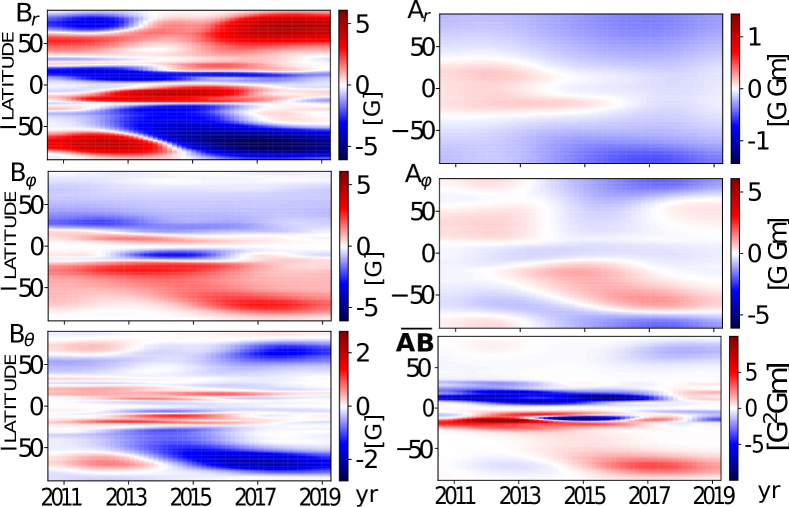
Figure 4: The time-latitude evolution of the large-scale magnetic field : $\bar{B}_{r}$, $\bar{B}_{\phi}$, and $\bar{B}_{\theta}$, as well as the large-scale vector-potential components $\bar{A}_{r}$ and $\bar{A}_{\phi}$, the total magnetic helicity density $\overline{\mathbf{{A}\cdot\mathbf{{B}}}}$.

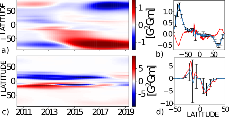
Figure 5: Magnetic helicity in Solar Cycle 24: a) The time-latitude evolution of the large-scale magnetic helicity density, $\mathbf{\overline{A}\cdot\mathbf{\overline{B}}}$; b) the mean latitudinal profile of the large-scale magnetic helicity density with 95$\%$ confidence interval for the standard error, the red line shows the average profile for the first half of the cycle including CR2097-2156; c) shows the same as (a) for the azimuthal averaging of the small-scale magnetic helicity density $\mathbf{\overline{a\cdot\mathbf{b}}}=\overline{\mathbf{{A}\cdot\mathbf{{B}}}}-\mathbf{\overline{A}\cdot\mathbf{\overline{B}}}$; d) shows the same as (b) for the $\mathbf{\overline{a\cdot\mathbf{b}}}$.

5 Discussion and Conclusions

Here, we propose a novel approach to reconstruct the surface magnetic helicity density on the Sun and sun-like stars. The magnetic vector potential is determined via decomposition of vector magnetic field in the toroidal and poloidal components. The method is applied to study the evolution of magnetic helicity density of large- and small-scale fields in solar cycle 24.

Our results show that at the beginning if cycle 24, the large- and small-scale magnetic helicities are opposite in sign to each other, and both show the hemispheric asymmetry in sign. This is in agreement with the magnetic helicity conservation theory (Frisch et al., 1975), which predicts the sign of variations of the small-scale magnetic helicity density, $\mathbf{\overline{a\cdot\mathbf{b}}}$ should be opposite to the sign of the large-scale helicity. However, in the declining phase of cycle 24 the large-scale polar magnetic field shows the negative (positive) magnetic helicity in the North (South), which is the same in sign as the helicity of solar active regions (small-scale field). Apparently, in the polar regions the large-scale helicity, $\mathbf{\overline{A}\cdot\mathbf{\overline{B}}}$, changed the sign near the solar maximum. The dynamo models predict that both $\mathbf{\overline{A}\cdot\mathbf{\overline{B}}}$ and $\mathbf{\overline{a\cdot\mathbf{b}}}$ can change sign in course of the solar cycle due to other sources of the magnetic helicity evolution like the turbulent eddy diffusivity of the large-scale magnetic field (Kleeorin & Ruzmaikin, 1982; Pipin et al., 2013; Sokoloff et al., 2013). Another possible reason is the magnetic helicity flux escape from the solar surface (Berger & Ruzmaikin, 2000). We also note that dynamo models of (Pipin et al., 2013) predict another polar inversion of the large-scale magnetic helicity models during solar minima. Thus, we expect that the magnetic helicity of large-scale (polar field) will reverse its sign again around the solar minimum, which would restore the hemispheric helicity rule to the same condition as it was at the beginning of cycle 24.

The amplitude of magnetic helicity of large-scale fields is significantly (an order of magnitude) smaller as compared with helicity of small-scale (active region) fields. Thus, active regions appear to be the major contributors to magnetic helicity observed on the visible solar surface (photosphere). This is further supported by the fact that the emergence of a single (large) active region could affect the hemispheric preference in sign of helicity for some Carrington rotations.

In our data we see that the magnetic helicity density of the large- and small-scale fields often show the same sign in each hemisphere. In our opinion this can be due to a bi-modal distribution of the large-scale toroidal magnetic field on the solar surface. Indeed, we see the two components of the toroidal magnetic field: one is near equator and another is in the mid latitudes. The near equatorial toroidal field is originated from sunspots. The origin of the mid-latitude toroidal field is unclear. This component of the large-scale field can results into mono-helical over the scales magnetic field distributions in the each hemisphere. The evolution of the large-scale magnetic field and its vector potential results in a complicated magnetic helicity evolution. In the data, it is seen that the southern hemisphere was close to the bi-helical state during the growing phase of the solar cycle, from 2010 to 2012. The northern hemisphere, except the polar region, shows the same sign of the magnetic helicity density for the large- and small-scale field during that period. Another source of violation of the hemispheric helicity rule is the asymmetric about equator development of solar cycle 24. This results in the equatorial parity breaking in the large-scale magnetic field and vector potential components. In particular, the obtained evolution of $\bar{A}_{\phi}$ is different from previous results by Blackman & Brandenburg (2002) and Pipin & Pevtsov (2014).

The hemispheric helicity rule and bi-helical distributions of the solar magnetic fields are essential properties of the solar dynamo operating in the convection zone. We find that in solar cycle 24 these properties of solar dynamo show a complicated evolution in the way which is not expected in any current dynamo model. The suggested method of the magnetic helicity reconstruction can be applied to other stars where the low-degree modes of the vector magnetic field distributions, such as determined in Vidotto et al. (2018), can be used to calculate the magnetic vector potential and magnetic helicity density of the large-scale stellar magnetic field.

References

- Balasubramaniam & Pevtsov (2011) Balasubramaniam, K. S., & Pevtsov, A. 2011, in Proc. SPIE, Vol. 8148, Solar Physics and Space Weather Instrumentation IV, 814809
- Bao & Zhang (1998) Bao, S., & Zhang, H. 1998, ApJ, 496, L43, doi: 10.1086/311232
- Berger & Hornig (2018) Berger, M. A., & Hornig, G. 2018, Journal of Physics A Mathematical General, 51, 495501, doi: 10.1088/1751-8121/aaea88
- Berger & Ruzmaikin (2000) Berger, M. A., & Ruzmaikin, A. 2000, J. Geophys. Res., 105, 10481, doi: 10.1029/1999JA900392
- Blackman & Brandenburg (2002) Blackman, E. G., & Brandenburg, A. 2002, ApJ, 579, 379, doi: 10.1086/342705
- Blackman & Brandenburg (2003) —. 2003, ApJ, 584, L99, doi: 10.1086/368374
- Brandenburg et al. (2017) Brandenburg, A., Petrie, G. J. D., & Singh, N. K. 2017, ApJ, 836, 21, doi: 10.3847/1538-4357/836/1/21
- Brandenburg & Subramanian (2005) Brandenburg, A., & Subramanian, K. 2005, Phys. Rep., 417, 1, doi: 10.1016/j.physrep.2005.06.005
- Choudhuri et al. (2004) Choudhuri, A. R., Chatterjee, P., & Nandy, D. 2004, ApJ, 615, L57, doi: 10.1086/426054
- Frisch et al. (1975) Frisch, U., Pouquet, A., Léorat, J., & A., M. 1975, J. Fluid Mech., 68, 769
- Hagino & Sakurai (2005) Hagino, M., & Sakurai, T. 2005, Publ. Astron. Soc. Japan, 57, 481
- Kleeorin & Ruzmaikin (1982) Kleeorin, N. I., & Ruzmaikin, A. A. 1982, Magnetohydrodynamics, 18, 116
- Krause & Rädler (1980) Krause, F., & Rädler, K.-H. 1980, Mean-Field Magnetohydrodynamics and Dynamo Theory (Berlin: Akademie-Verlag), 271
- Liu et al. (2017) Liu, Y., Hoeksema, J. T., Sun, X., & Hayashi, K. 2017, Sol. Phys., 292, 29, doi: 10.1007/s11207-017-1056-9
- Longcope et al. (1998) Longcope, D. W., Fisher, G. H., & Pevtsov, A. A. 1998, ApJ, 507, 417, doi: 10.1086/306312
- Pesnell et al. (2012) Pesnell, W. D., Thompson, B. J., & Chamberlin, P. C. 2012, Sol. Phys., 275, 3, doi: 10.1007/s11207-011-9841-3
- Pevtsov et al. (2014) Pevtsov, A. A., Berger, M. A., Nindos, A., Norton, A. A., & van Driel-Gesztelyi, L. 2014, Space Sci. Rev., 186, 285, doi: 10.1007/s11214-014-0082-2
- Pevtsov et al. (1995) Pevtsov, A. A., Canfield, R. C., & Metcalf, T. R. 1995, ApJ, 440, L109, doi: 10.1086/187773
- Pevtsov et al. (2008) Pevtsov, A. A., Canfield, R. C., Sakurai, T., & Hagino, M. 2008, ApJ, 677, 719, doi: 10.1086/533435
- Pevtsov & Latushko (2000) Pevtsov, A. A., & Latushko, S. M. 2000, ApJ, 528, 999, doi: 10.1086/308227
- Pipin (2018) Pipin, V. 2018, VVpipin/2DSPDy 0.1.1, doi: 10.5281/zenodo.1413149
- Pipin & Kosovichev (2018) Pipin, V. V., & Kosovichev, A. G. 2018, ApJ, 867, 145, doi: 10.3847/1538-4357/aae1fb
- Pipin & Pevtsov (2014) Pipin, V. V., & Pevtsov, A. A. 2014, ApJ, 789, 21, doi: 10.1088/0004-637X/789/1/21
- Pipin et al. (2013) Pipin, V. V., Zhang, H., Sokoloff, D. D., Kuzanyan, K. M., & Gao, Y. 2013, MNRAS, 435, 2581, doi: 10.1093/mnras/stt1465
- Pouquet et al. (1975) Pouquet, A., Frisch, U., & Léorat, J. 1975, J. Fluid Mech., 68, 769
- Raedler (1986) Raedler, K.-H. 1986, Astronomische Nachrichten, 307, 89, doi: 10.1002/asna.2113070205
- Scherrer et al. (2012) Scherrer, P. H., Schou, J., Bush, R. I., et al. 2012, Sol. Phys., 275, 207, doi: 10.1007/s11207-011-9834-2
- Seehafer (1990) Seehafer, N. 1990, Sol. Phys., 125, 219, doi: 10.1007/BF00158402
- Singh et al. (2018) Singh, N. K., Käpylä, M. J., Brandenburg, A., et al. 2018, ApJ, 863, 182, doi: 10.3847/1538-4357/aad0f2
- Sokoloff et al. (2013) Sokoloff, D., Zhang, H., Moss, D., et al. 2013, in Proceedings of the International Astronomical Union, Vol. 8, Symposium S294 (Solar and Astrophysical Dynamos and Magnetic Activity), ed. A. G. Kosovichev, E. de Gouveia Dal Pino, & Y. Yan, 313–318
- Stenflo & Guedel (1988) Stenflo, J. O., & Guedel, M. 1988, A&A, 191, 137
- Vidotto et al. (2018) Vidotto, A. A., Lehmann, L. T., Jardine, M., & Pevtsov, A. A. 2018, MNRAS, 480, 477, doi: 10.1093/mnras/sty1926
- Virtanen et al. (2019) Virtanen, I. I., Pevtsov, A. A., & Mursula, K. 2019, A&A, 624, A73, doi: 10.1051/0004-6361/201834895
- Wieczorek & Meschede (2018) Wieczorek, M., & Meschede, M. 2018, Geochemistry, Geophysics, Geosystems, 19, 2574, doi: 10.1029/2018GC007529
- Zhang et al. (2010) Zhang, H., Sakurai, T., Pevtsov, A., et al. 2010, MNRAS, 402, L30, doi: 10.1111/j.1745-3933.2009.00793.x