Interpreting the distributions of FRB observables

Abstract

Fast radio bursts (FRBs) are short-duration radio transients of unknown origin. Thus far, they have been blindly detected at millisecond timescales with dispersion measures (DMs) between 110–2600 pc cm^-3. However, the observed pulse width, DM, and even brightness distributions depend strongly on the time and frequency resolution of the detection instrument. Spectral and temporal resolution also significantly affect FRB detection rates, similar to beam size and system-equivalent flux density (SEFD). I discuss the interplay between underlying FRB properties and instrumental response, and provide a generic formalism for calculating the observed distributions of parameters given an intrinsic FRB distribution, focusing on pulse width and DM. I argue that if there exist many FRBs of duration $<<$ 1 ms (as with giant pulses from Galactic pulsars) or events with high DM, they are being missed due to the deleterious effects of smearing. I outline how to optimise spectral and temporal resolution for FRB surveys that are throughput-limited. I also investigate how such effects may have been imprinted on the distributions of FRBs at real telescopes, like the different observed DMs at ASKAP and Parkes. Finally, I discuss the impact of intrinsic correlations between FRB parameters on detection statistics.

1 Introduction

Fast radio bursts (FRBs) are a new class of extragalactic radio transient whose origins remain a mystery. The dispersion measures (DM) of observed FRBs have been between 110–2600 pc cm^-3, significantly exceeding the expected contribution from the Milky Way along their respective lines-of-site. Roughly 70 sources of FRBs have been found to date (Petroff et al., 2016). They have now been discovered at six different telescopes around the world, in bands between 400 MHz and 8 GHz (Lorimer et al., 2007; Thornton et al., 2013; Spitler et al., 2014; Masui et al., 2015; Caleb et al., 2017; Shannon et al., 2018; CHIME/FRB Collaboration et al., 2019a; Gajjar et al., 2018). Of the known FRB-emitting sources, two (Spitler et al., 2016; CHIME/FRB Collaboration et al., 2019b) have been found to repeat; all others have been once-off events. Blindly-detected events have had duration 0.64–21 ms, but thanks to coherent dedispersion of dumped raw voltage data (Michilli et al., 2018; Farah et al., 2018) and pulse fitting (Ravi et al., 2016; CHIME/FRB Collaboration et al., 2019a), some FRBs are known to have structure on microsecond timescales.

Several broad-band, wide-field surveys are expected to be transformative for the FRB field, and are presently either operational or in the late commissioning stage. These include the Canadian Hydrogen Intensity Mapping Experiment (CHIME; CHIME/FRB Collaboration et al. (2018)), the Australian Square Kilometre Array Pathfinder (ASKAP; Bannister et al. (2017)), UTMOST (Bailes et al., 2017), the APERture Tile in Focus (Apertif; van Leeuwen (2014)), and Meer TRAnsients and Pulsars (MeerTRAP) (Sanidas et al., 2017). As the field transitions from small-number statistics to hundreds or thousands of new FRBs per year, our statistical tools must mature accordingly. This will include understanding the interplay between the underlying source distribution, our instruments, and FRB detection statistics. The underlying source distribution refers to intrinsic physical properties of the FRB population, including energetics, redshift distribution, and spectral behaviour. Detection statistics refers to FRB observables, such as the observed brightness distribution and event detection rates. The mapping between intrinsic and observed properties is central to this paper.

Several groups have considered brightness completeness effects in order to accurately calculate event rates (Keane & Petroff, 2015; Connor et al., 2016b). Others have studied the effects of the redshift, luminosity, and spectral index distributions of FRBs on their detected source counts (Oppermann et al., 2016; Caleb et al., 2016; Vedantham et al., 2016; Amiri et al., 2017; Niino, 2018). In Macquart & Ekers (2018b), the authors derive many of the relations between such physical properties from first principles for cosmological FRBs.

Less attention has been paid to the subtle ways in which instrumental response can affect the distributions of FRB observables, or how different temporal and spectral resolution can alter by orders-of-magnitude the detection rate at two otherwise-identical telescopes. These selection effects are particularly important for interpreting the observed DM and brightness statistics of FRBs, which contain information about their spatial and luminosity distributions. The new era of sensitive, wide-field surveys will require a low-level understanding of how to tease out the underlying DM distributions and source counts from what is observed. Beyond DMs, luminosities, and redshifts, such understanding will also enable us to constrain the intrinsic spectrum of FRBs, volumetric event rates, energy cut-offs, and intrinsic correlations between FRB variables. It will also affect various proposed FRB applications. For example, missing highly-dispersed events due to instrumental selection effects may preclude the use of FRBs in cosmology (McQuinn, 2014; Masui & Sigurdson, 2015; Madhavacheril et al., 2019).

In Sect. 2 of this paper I develop a generic formalism for calculating detection rates at a given instrument, based on the underlying FRB distribution. This includes a method for determining the observed distribution of an FRB parameter given its true distribution, where I focus here on pulse width and DM. I then discuss optimising time and frequency resolution on an instrument once something is known about the true distributions of DM, pulse width, and source counts. In Sect. 3 I apply these tools to real data and investigate how such effects might have been imprinted on the detection statistics of FRBs at telescopes such as ASKAP and Parkes. Finally, in Sect. 4 I investigate how correlations between FRB parameters can alter the relationship between the observed and true distribution of FRBs.

2 Detection statistics

The detection rate, $\mathcal{R}$, of a blind single-pulse survey is given by an integral of differential event rate over all relevant parameters, $\mathbf{\lambda}=[{\lambda_{1},\ldots,\lambda_{m}}]$, in the region of phase space, $\mathbf{\Lambda}$, to which that survey is sensitive,

$$\mathcal{R}=\int\cdots\int_{\mathbf{\Lambda}}\,n(\lambda_{1},\lambda_{2},\ldots,\lambda_{m})\,d\lambda_{1}\!\cdots d\lambda_{m}.$$ (1)

Here $n(\lambda_{j})$ is the number density of events around parameter $\lambda_{j}$. Formally, this is a differential intrinsic event rate,

$$n(\lambda_{j})\equiv\frac{\mathrm{d\,N}}{\mathrm{d}\lambda_{j}}.$$ (2)

For example, $n(s)$ would be the differential brightness distribution of FRBs before any selection effects. As I show in Sect. 4, correlations between the different distributions $n(\lambda_{j})$ can affect detection statistics.

Typically, FRB detection rates have been computed using only beam size and a brightness threshold, where the integral is calculated over location on the sky, denoted by the unit vector, $\hat{k}$, and a measure of pulse strength, $s$, whether flux density, fluence, or signal-to-noise ratio (S/N). The equation,

$$\mathcal{R} =\int\displaylimits_{4\pi}\int\displaylimits_{s_{\mathrm{m}}}n(\hat{k},s)\,\mathrm{d}\hat{k}\mathrm{d}s$$ (3)

is often simplified with the assumptions that the radio beam is a two-dimensional top hat, the events are isotropic within a beam, and the brightness distribution is a power-law such that, $n(s)\propto s^{-\alpha-1}$. This results in the familiar equation,

$$\mathcal{R} \propto\Omega\,s_{\mathrm{m}}^{-\alpha},$$ (4)

where $\Omega$ is a measure of the telescope’s field of view (FoV), $s_{\mathrm{m}}$ is a minimum detectable brightness, and $\alpha$ is the source counts power-law index, such that

$$\alpha\equiv\frac{\partial{\log n(>s)}}{\partial{\log s}}.$$ (5)

Several authors have highlighted the importance of integrating over the full beam, due to the dependence of $s_{\mathrm{m}}$ on where in that beam the FRB arrives (Vedantham et al., 2016; Lawrence et al., 2017; Macquart & Ekers, 2018a). By considering the full beam,

$$\mathcal{R}=\int\displaylimits_{4\pi}n(\hat{k})\!\!\int\displaylimits_{s_{\mathrm{m}}(\hat{k})}s^{-\alpha-1}\,\mathrm{d}s\,\mathrm{d}\hat{k},$$ (6)

one can account for the detection of bright, but rare, events in the side-lobes, whose sky coverage are much larger than the primary beam. This is valuable for estimating FRB sky rates and for comparing detection rates between surveys with different beam shapes. The resultant brightness distribution shape is not affected by the beam response so long as the underlying source counts distribution is a power-law and the dynamic range between the brightest and dimmest event is large. If one of those conditions is not met, the observed brightness distribution’s logarithmic slope can deviate from that of the input, and its functional form can stray from power-law.

However, Eq. 4 not only neglects beam effects, but ignores the distributions of several other important parameters and the way they differentially affect surveys with disparate properties. If I also include DM and intrinsic pulse width, $t_{i}$, on top of sky location and brightness, I have $\mathbf{\lambda}=[\hat{k},s,\mathrm{DM},t_{i}]$ and the integral in Eq. 1 becomes,

$$\mathcal{R} =\int n(\hat{k},s,\mathrm{DM},t_{i})\,\mathrm{d}\hat{k}\,\mathrm{d}s\,\mathrm{dDM}\,\mathrm{d}t_{i}$$ (7)

$$=\int\displaylimits_{4\pi}n(\hat{k})\int\displaylimits_{0}^{\infty}n(t_{i})\!\int\displaylimits_{\mathrm{DM_{min}}}^{\mathrm{DM_{max}}}\!n(\mathrm{DM})\,\int\displaylimits_{s^{\prime}_{\mathrm{m}}}^{\infty}n(s)\,\mathrm{d}S\,\mathrm{dDM}\,\mathrm{d}t_{i}\,\mathrm{d}\hat{k}.$$ (8)

This equation calculates the number of detectable events per unit time for a survey with $\mathrm{DM_{min}}$, $\mathrm{DM_{max}}$, given an underlying FRB distribution described by $n(t_{i})$, $n(\mathrm{DM})$, and $n(s)$. Crucially, the minimum detectable single-pulse brightness, $s^{\prime}_{\rm{m}}$, depends on all of the former inputs. It will depend on where in the beam the FRB arrives; it is also increased by the deleterious effects of temporal smearing due to intra-channel dispersion and the instrument’s finite time sampling.

These effects all reduce detection rate and are not necessarily small corrections: If the functional form of $n(t_{i})$ were similar to $n(s)$ (source counts), then halving one’s instrumental smearing would have as much impact as doubling the telescope’s collecting area or cutting in half its system temperature with a cooled receiver.

In this paper I consider two simple intrinsic DM distributions. The first traces the star-formation rate, which is a top-heavy distribution with many highly-dispersed events. I follow Niino (2018) in using a DM redshift relation give by,

$$\mathrm{DM}(z)=1000\,z\,\,\,\mathrm{pc\,cm}^{-3}.$$ (9)

Combining this with an FRB number density in redshift, $\rho(z)$, and the comoving volume element per redshift bin, $\frac{dV}{dz}$, the number of FRBs per DM is,

$$\frac{dn}{d\mathrm{DM}}=\frac{\rho(z)}{(1+z)}\frac{dV}{dz}\frac{dz}{d\mathrm{DM}},$$ (10)

where I use,

$$\rho(z)=\rho_{SFR}(z)\propto\frac{(1+z)^{2.5}}{1+((1+z)/2.9)^{5.6}}$$ (11)

from Madau & Dickinson (2014). The second is a Gaussian distribution peaking at 1000 pc cm^-3 with standard deviation 500 pc cm^-3, corresponding to a scenario where FRBs are primarily dispersed local to the source. In reality, the intrinsic DM distribution of FRBs will depend on their luminosity function (Niino, 2018; Macquart & Ekers, 2018a). But by using both a top- and bottom-heavy DM distribution, most plausible outcomes are spanned. In the following subsections, I consider the implications of Eq. 8 and the aforementioned DM distributions on the observed properties of FRBs in the presence of real instrumental effects.

2.1 Temporal smearing

The observed pulse width is a quadrature sum of the intrinsic pulse width, the dispersion-smearing timescale, and the sampling time (Cordes & McLaughlin, 2003),

$$t_{\mathrm{obs}}=\sqrt{\,t_{i}^{2}+t^{2}_{\mathrm{DM}}+t^{2}_{s}}.$$ (12)

I define the intrinsic width, $t_{i}$, not as the emitted pulse width, but as the duration of the pulse when it arrives at a radio telescope, before instrumental smearing.

$$t_{i}=\sqrt{\,t^{2}_{e}(1+z)^{2}+\tau^{2}}.$$ (13)

Here, the FRB from redshift $z$ had a rest-frame emission width at the source, $t_{e}$, and has a final scattering timescale $\tau$.

I do not attempt to model the temporal scattering, emission width, or FRB redshift distributions, and instead only include the understood phenomenon of instrumental pulse broadening. I ignore the discretisation of pulse widths introduced by single-pulse search software (Keane & Petroff, 2015), which usually choose a finite set of boxcar widths. I have also assumed that intra-channel dispersion smearing produces a Gaussian profile, even though it is closer to the intrinsic profile convolved with a box-car. An upcoming FRB detection software challenge will offer more realistic insights into such single-pulse search effects .

Finite frequency resolution leads to a dispersion delay within individual frequency channels, which artificially broadens a dispersed pulse. This intra-channel dispersion smearing is linear in DM as,

$$t_{\mathrm{DM}}=\rm{A\,DM},$$ (14)

where the proportionality constant is

$$\mathrm{A}=8.3\left(\frac{\Delta\nu}{1\,\mathrm{MHz}}\right)\left(\frac{\nu_{c}}{1\,\mathrm{GHz}}\right)^{-3}\,\,\mu\mathrm{s},$$ (15)

and depends on the instrument’s frequency resolution, $\Delta\nu$, and central observing frequency, $\nu_{c}$. The relevant timescales in this paper are listed in Table. 1.

The minimum brightness detection threshold in the absence of broadening is denoted by, $s_{m,o}$. This threshold will be transformed by the beam response and the smearing terms in the following way,

$$s^{\prime}_{\mathrm{m}}=s_{\mathrm{m},o}\,\,b(\hat{k})^{-1}\,\left(\frac{t_{i}^{2}+t_{s}^{2}+\mathrm{A}^{2}\,\mathrm{DM}^{2}}{t_{i}^{2}}\right)^{1/2},$$ (16)

where the beam response, $b(\hat{k})$, is assumed to be unity on-axis.

Ignoring beam effects for now, one can investigate how event detection rates depend on the sensitivity reduction from temporal smearing (for beam effects, see, e.g., (Ravi, 2019; James et al., 2019)). Taking $\mathcal{R}_{\hat{k}}$ to be the detection rate per unit solid angle and evaluating the brightness component of the integral in Equation 16 with a power-law $n(s)=s^{-\alpha-1}$, one gets,

Table 1: Relevant FRB width timescales

$t_{e}$	restframe emitted width
$\tau$	scattering timescale
$t_{i}$	intrinsic width (at receiver)
$t_{\mathrm{D}M}$	intra-channel dispersion-smearing timescale
$t_{s}$	sampling time
$t_{\mathrm{o}bs}$	final observed pulse width

$$\mathcal{R}_{\hat{k}}=\frac{s_{\mathrm{m},o}^{-\alpha}}{\alpha}\int\displaylimits_{0}^{\infty}\!n(t_{i})\!\!\int\displaylimits_{\mathrm{DM_{min}}}^{\mathrm{DM_{max}}}\!\!\!n(\mathrm{DM})\left(\frac{t_{i}^{2}+t_{s}^{2}+\mathrm{A}^{2}\,\mathrm{DM}^{2}}{t_{i}^{2}}\right)^{-\alpha/2}\!\!\!\!\!\!\mathrm{dDM}\,\mathrm{d}t_{i}.$$ (17)

Because $s^{\prime}_{m}\geq s_{m,o}$ and $\alpha$ is positive, the detection rate will always be decreased by the finite time and frequency resolutions of real telescopes. The degree to which FRBs are “missed” due to smearing will depend on their underlying brightness, DM, and width distributions. The latter two have been neglected in the FRB statistics literature, but are very important if there exist considerable numbers of narrow and high-DM FRBs.

Qualitatively, if $\alpha$ is large and the brightness distribution is steep, a greater fraction of events will be missed due to smearing because there are many events close to the detection threshold that will fall below it. If the distribution of intrinsic pulse widths, $n(t_{i})$, is such that there are lots of events narrower than the sampling or the dispersion-smearing timescale, surveys with poor time and frequency resolution will take a large hit in their event rates. The same is true if the underlying DM distribution of FRBs is weighted towards highly dispersed events. However, it is not just the overall detection rates that will be affected: The observed DM and brightness distributions, as well as the inter- and intra-survey correlations between those quantities, will also be changed.

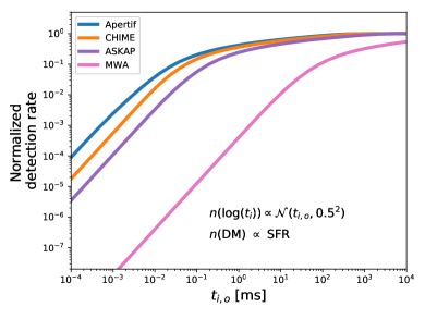
Figure 1: The FRB detection rate at several surveys normalised to their rate if they had perfect time and frequency resolution. This value is plotted as a function of mean pulse width, $t_{i,o}$, of a lognormal intrinsic width distribution with standard deviation $\log 0.5$. The DM distribution follows the star-formation rate.

The 2D integral in Eq. 17 is calculated for Fig. 1 using a DM distribution that follows the star-formation rate (SFR) and a lognormal intrinsic pulse width distributions with varying means. Clearly the FRB detection rate of an instrument depends strongly on the underlying pulse widths, drastically so in the case of low-resolution back-ends. This must be accounted for when rates between surveys are compared, or when detection rates are forecasted. The survey parameters assumed in this paper are listed in Table. 2.

2.2 Observed DM distribution

The combination of temporal smearing and the unknown, intrinsic pulse width and DM distributions will differentially affect detection rates at each FRB survey. They will also alter the shape of distributions of various observables, including DM. One can calculate the fraction of recovered events, $\eta$, at each DM, given a brightness distribution, intrinsic pulse width distribution, and instrumental parameters. Starting from Equation 17, this is,

$$\eta(\mathrm{DM}) \equiv\frac{n_{\mathrm{obs}}\left(\mathrm{DM}\right)}{n\,(\mathrm{DM})}$$ (18)

$$=\frac{1}{C}\int\displaylimits_{0}^{\infty}\!n(t_{i})\,\left(\frac{t_{i}^{2}+t_{s}^{2}+\mathrm{A}^{2}\,\mathrm{DM}^{2}}{t_{i}^{2}}\right)^{-\alpha/2}\mathrm{d}t_{i}$$ (19)

where $C$ is a normalising constant representing the number of events that would have been detected with perfect time and frequency resolution,

$$C\equiv\int\displaylimits_{0}^{\infty}\!n(t_{i})\,\mathrm{d}t_{i}.$$ (20)

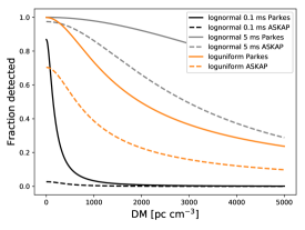
Figure 2: The fraction of events detected by Parkes (solid) and ASKAP (dashed) compared to the same survey without smearing, plotted as a function of DM for three different intrinsic pulse width distributions. The log-normal curves have standard deviation $0.25$. Without knowing the intrinsic width distribution, one cannot know the transfer function between true and observed DMs.

In Fig. 2 I show how the distributions of FRB parameters intermix with instrumental effects and can significantly affect both detection rates and observed DM distributions. The fraction of recovered FRBs, $\eta$, is plotted as a function of DM for Parkes and ASKAP, using three different intrinsic pulse width distributions: lognormal, peaked at 100 $\mu$s; lognormal, peaked at 5 ms; and loguniform. The lognormal integrals are calculated over four order-of-magnitude centered on the mean. The loguniform distribution is summed from 0.01–100 ms.

Clearly, a large fraction of FRBs are missed at DM $\gtrapprox$ 1000 pc cm^-3 for many width distributions, especially using ASKAP’s current temporal and spectral resolution. It should not be surprising that all $\sim$ 70 FRBs have had DM $\leq$ 2600 pc cm^-3: Either such high-DM events truly are rare or they are common and smeared below our detection thresholds. And given the intrinsic pulse widths of FRBs need not be that narrow for current back-ends to miss them, it seems likely that many high-DM events are indeed being lost. Highly-dispersed bursts probe either the most dense FRB environments or the highest redshifts, so they will be of great scientific interest. Therefore, surveys with the ability to trade time resolution for higher frequency resolution could alter their DM response function, making their instrument more sensitive to high-DM events. I discuss such trade-offs in Sect. 2.4.

If the DM distribution of FRBs is top-heavy (i.e. lots of highly dispersed events), then the detection rates of all current surveys are considerably suboptimal. Perhaps more importantly, $\eta$ represents a transfer function between the true and observed DM distribution, and its shape depends strongly on the instrument’s time and frequency resolution. In Sect. 3 I investigate whether this could produce the DM/fluence relationship found between ASKAP and Parkes (Shannon et al., 2018).

Table 2: Survey parameters used in this paper. UTMOST increased its time/frequency resolution in 2018 after its first three detections.

Survey	$t_{s}$ [ms]	$\Delta\nu$ [MHz]	$K$ [ms MHz]	$\nu_{c}$ [GHz]
ASKAP	1.3	1.0	1.3	1.4
Parkes	0.064	0.39	0.19	1.4
Apertif	0.041	0.195	0.08	1.4
CHIME	0.983	0.024	0.024	0.6
UTMOST2017†	0.655	0.780	0.511	0.82
UTMOST2018∗	0.327	0.097	0.032	0.82
MWA	500	1.24	620	0.185

2.3 Observed width distribution

With pulse duration, calculating the observed distribution is less trivial than for DMs because widths are transformed at the instrument by smearing. In contrast, the observed DM of a given FRB is the same at the DM with which is arrives at our receivers. The distribution of the smeared widths is a probability density function (PDF) of a variable that has undergone a non-linear transformation. Nonetheless, in many cases the new distribution can be solved analytically if the transformation is known, which it is for smearing.

If the PDF of a real random variable is known, the distribution of a function, $f$, of that variable can be calculated, as long as $f$ is invertible. In the case of FRB widths, one is concerned with the final distribution of observed pulse duration,

$$n(t_{\mathrm{obs}})=n_{t_{\mathrm{obs}}}(f(t_{i})).$$ (21)

The function $f$ is given by Eq. 12, and its inverse is,

$$t_{i}=f^{-1}(t_{\mathrm{obs}})=\sqrt{\,t_{\mathrm{obs}}^{2}-t_{s}^{2}-t_{DM}^{2}}.$$ (22)

The underlying FRB pulse width distribution, $n_{t_{i}}$, is transformed into an observed distribution as,

$$n(t_{obs})=n_{t_{i}}\left(f^{-1}(t_{obs})\right)\frac{df^{-1}}{dt_{obs}},$$ (23)

Differentiating $f^{-1}$ and inserting it into Eq. 23, one finds that the resultant observed width distribution at each DM is,

$$n(t_{\mathrm{obs}})=n_{t_{i}}\left(\sqrt{\,t_{\mathrm{obs}}^{2}-t_{s}^{2}-t_{DM}^{2}}\right)\frac{t_{\mathrm{obs}}}{\sqrt{\,t_{\mathrm{obs}}^{2}-t_{s}^{2}-t_{DM}^{2}}}.$$ (24)

As an example, if the underlying width distribution is uniform, then $n_{t_{i}}(x)$ is constant and the observed pulse widths have

$$n(t_{obs})=\frac{t_{obs}}{\sqrt{\,t_{obs}^{2}-t_{s}^{2}-t_{DM}^{2}}}.$$ (25)

If the intrinsic width distribution is lognormal, one gets

$$n(t_{obs})=\mathrm{exp}\left\{-\log^{2}\left(\sqrt{\,t_{obs}^{2}-t_{s}^{2}-t_{DM}^{2}}\right)\right\}\frac{t_{obs}}{\sqrt{\,t_{obs}^{2}-t_{s}^{2}-t_{DM}^{2}}}.$$ (26)

The intrinsic and observed width distributions are shown in solid and dashed curves, respectively, in Fig. 3. The plot assumes DM smearing is significantly less than the sampling time, in this case, so no DM distribution was assumed. These functions are not defined for $t_{obs}\leq\sqrt{t_{s}^{2}+t_{DM}^{2}}$ because one cannot detect an FRB that is narrower than the smearing timescale. That is why the observed PDF in Fig. 3 asymptotes to the instrumental smearing width, effectively limiting the detection width to the quadrature sum of dispersion smearing and sampling time.

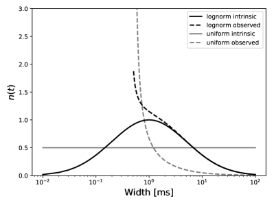
Figure 3: The underlying (solid) and observed (dashed) pulse width distributions for a hypothetical survey with 0.5 ms sampling time. The black and grey curves represent a log-normal and uniform input pdf, respectively. This figure assumes dispersion smearing is small compared to the sampling time.

2.4 Optimising survey resolution

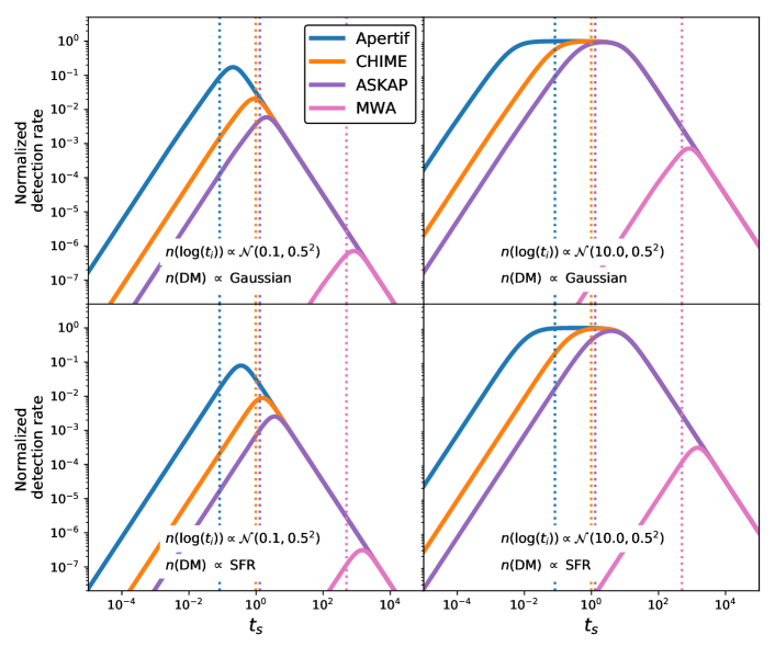
Figure 4: The FRB detection rate of several surveys normalised to their detection rate if they had perfect time and frequency resolution, plotted as a function of sampling time. These are not absolute rates to be compared between surveys, but a measure of their individual incompleteness due to smearing. I assume that each survey’s temporal and spectral resolution are limited by data rates, meaning $t_{s}\Delta\nu$ is constant. Dashed vertical lines indicate each telescope’s nominal sampling time; the curve’s peak indicates an optimal sampling time for a given DM and intrinsic pulse width distribution.

Modern digitisers sample the sky’s electric field at an enormous rate, providing very fine temporal resolution at the telescope’s front-end of roughly the inverse bandwidth. However, signal processing constraints mean data must be binned down in both time and frequency after the data are squared or correlated. Such throughput limitations often lead to the constraint that the product of the time and frequency resolution must be constant,

$$\Delta\nu\,t_{s}\equiv K\,\,\,[\mathrm{MHz\,ms}].$$ (27)

In other words, if one wants twice as many frequency channels, one must lose a factor of two in time resolution.

Each survey will have its own value of $K$, and depending on the underlying DM, brightness, and pulse width distributions, a pair of ($t_{s}$, $\Delta\nu$) can be chosen to optimise FRB detection rate. This is done by differentiating $\mathcal{R}_{\hat{k}}$ in Eq. 17 with respect to $t_{s}$ after replacing $\Delta\nu$ with $K/t_{s}$. In Fig. 4 I plot the FRB detection rates for several surveys, assuming they are constrained by current spectral and temporal resolution, as a function of sampling time. As before, I have used simplifying assumptions about the intrinsic width and DM distributions. The two toy models for $n(\mathrm{DM})$, described in Sect. 2, assume standard candles and no $k$-corrections. I also assume no correlations between any input variables, such as brightness, DM, and intrinsic width.

Fig. 4 calculates rates by summing over all DMs and intrinsic pulse widths to find the largest overall detection rate. However, depending on the survey’s scientific interests, the goal may not be simply to maximize the number of detected events, but to maximize sensitivity to certain types of bursts. For example, high-DM events come either from the greatest distances or the most dense environments, so surveys may want to upchannelise at the expense of time resolution. A further constraint exists for telescopes that search formed beams in realtime, like Apertif and CHIME. If the conserved quantity in data rate is instead $t_{s}\Delta\nu\,N_{\mathrm{beam}}$, then the brightness distribution parameter $\alpha$ becomes more important. The trade-off between FoV and sensitivity is largely determined by source counts. If $\alpha$ turns out to be large and the brightness distribution is steep, it may make sense to sacrifice number of beams for better temporal and spectral resolution.

2.5 Scattering

Instead of attempting to model temporal scattering of FRBs explicitly, I have folded it into the intrinsic pulse width $t_{i}$. This is because this paper is concerned primarily with instrumental selection effects on DM, width, and brightness, so astrophysical pulse broadening will simply alter the underlying width distribution of FRBs, $n(t_{i})$. Nonetheless, scattering is strongly frequency dependent ($\tau\propto\nu^{-4}$), meaning $n(t_{i})$ will be a function of frequency. One should therefore expect the true widths of FRBs at low frequencies to be wider than at higher frequencies and surveys at different bands will suffer the deleterious effects of smearing differently. For this reason, when the same $n(t_{i})$ is used for surveys observing at different bands, as in Fig. 4, it may be prudent to not compare the telescopes to one another directly, in case scattering significantly changes the distributions of $t_{i}$ as a function of frequency. As an example, if CHIME continues to find that a significant fraction of FRBs between 400–800 MHz are scattered, the optimisations described in this section may be less valuable there than at 1400 MHz. To date, details about the scattering statistics of FRBs are difficult to constrain. CHIME found a majority of events (CHIME/FRB Collaboration et al., 2019a) significantly scattered (8/13), but ASKAP found evidence for scattering in just 3 of 20 events (Shannon et al., 2018). Slightly less than half of Parkes FRBs are scattered (Petroff et al., 2016; Ravi, 2019), but at this point we cannot know if such differences are due to scattering trends in frequency or DM, and which are due to instrumental selection effects.

3 FRB Data

3.1 Observed width distribution

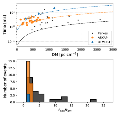
Figure 5: The observed pulse widths of FRBs. The top panel shows width as a function of DM for three surveys along with their theoretical smearing curves ($t_{sm}$). The bottom panel shows the distributions of observed widths for the same three surveys, normalised by the fundamental smearing limit at their respective FRBs and with their back-ends. Nearly all ASKAP and UTMOST FRBs ‘hug’ the smearing curve.

To date, blind FRB detections have had widths between 0.64–21 ms, which is why FRBs are often described as millisecond-duration pulses. These detections were made with instruments whose smearing timescale is $\sim$ millisecond at the relevant DMs, so little is known about the lower-limit of FRB widths. In Fig. 5 I plot their observed widths as a function of DM as well as the distribution of their widths normalised by the smearing timescale, $t_{sm}=\sqrt{t^{2}_{s}+t^{2}_{\rm DM}}$.

The values $t_{\rm obs}$ plotted in Fig. 5 are the detected pulse durations, typically boxcar widths used by dedispersion codes blindly searching intensity data. The UTMOST FRBs are the telescope’s first three detections, made before the system’s time and frequency resolution were improved (Caleb et al., 2017). The Parkes and ASKAP sources come from FRBCAT, with 21 and 23 FRBs respectively (Petroff et al., 2016). I do not include the 13 pre-commissioning CHIME FRBs because their reported pulse duration is not a detected boxcar width, but the fit from a Markov Chain Monte Carlo (MCMC) procedure; CHIME’s large fractional bandwidth allows for the separation of frequency-dependent broadening effects like dispersion smearing and scattering.

The bursts hug closely their respective temporal smearing curves shown in the upper panel. The histogram in the bottom panel suggest that there are many FRBs narrower than these telescope’s smearing timescale, and the observed distributions are qualitatively similar to the analytical curves in Fig. 3.

Despite the millisecond widths of blind detections, it is known that FRBs have structure on much shorter timescales. This is because FRBs can be coherently dedispersed if voltage data are available, allowing for near-perfect time and frequency resolution. The first two sources to be coherently dedispersed offer insight into the temporal properties of FRBs. FRB121102 was the first source found to repeat, and its coherently dedispersed bursts have been as narrow as $\leq$ 30$\mu$s (Michilli et al., 2018). FRB170827 was detected at UTMOST with incoherent dedispersion, but a voltage dump was triggered in real time. This allowed for coherent dedispersion that revealed microstructure of $\sim$ 30$\mu$s (Farah et al., 2018). Similarly, Ravi et al. (2016) argued that the spectral structure in FRB150807—which was unresolved even at 350 $\mu$s—implied that its time profile was dominated by structure of a few microseconds.

It is worth noting that while these are the narrowest FRB components ever detected, the full burst often lasts longer than the microstructure. Since they were found with incoherent back-ends with millisecond smearing timescales, both UTMOST and PALFA were biased to see FRBs whose duration aligned with their searchable boxcar widths. Until blind searches at 10s to 100s of microseconds are done, we will not know how many narrow FRBs exist.

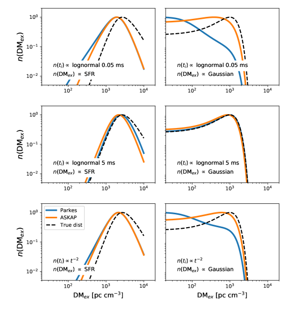
Figure 6: The simulated observed DM distribution for six combinations of intrinsic FRB widths and DMs. Each panel shows the distribution of detected DMs at Parkes (blue) and ASKAP (orange) as well as the underyling DM distribution (black, dashed). Each is normalised to peak at 1. The left column uses a true DM distribution that tracks the star-formation rate, and the right column is Gaussian with mean 1000 pc cm^-3, standard deviation 500 pc cm^-3. The first, second, and third rows use intrinsic width distributions that are lognormal with mean 0.05 ms, lognormal with mean 5 ms, and loguniform respectively.

3.2 ASKAP and Parkes

The observed extragalactic DM distribution differs significantly between Parkes FRBs and those detected with ASKAP, with lower DM_ex events found with the latter. In fly’s-eye mode, ASKAP is roughly 50 times less sensitive than Parkes and because FRB surveys have been flux-limited thus far, ASKAP necessarily detects much brighter FRBs than Parkes. Therefore, there may be evidence that extragalactic DM anti-correlates with brightness, which is expected for many luminosity functions in the cosmological FRB scenario (Shannon et al., 2018).

However, as shown in Section 2.2 the observed DM distribution is transformed by the system’s response, which are different at Parkes and ASKAP. The extent to which the observed DMs diverge will depend on the unknown true intrinsic pulse widths and DMs of the FRB population, and the time/frequency resolution and observing frequency of the instruments. Thus, one can ask the question, “Which underlying width/DM_ex distributions can produce such a discrepancy in the observed DMs that is purely due to instrumental smearing?”. In Fig. 6 I plot the normalised observed DM distributions at Parkes (blue) and ASKAP (orange) for six combinations of underlying width and DM_ex inputs, assuming Euclidean source counts. The left column uses a true DM_ex distribution (black, dashed curves) that traces the star-formation rate; the right column assumes a Gaussian intrinsic DM distribution, peaking at 1000 pc cm^-3. Each of the three rows corresponds to a different underlying width distribution.

I find that the the shape and scaling (detection rate) of the observed DM distribution can differ greatly from the true DM distribution. The observed distributions at Parkes and ASKAP can also vary significantly, due to their different time and frequency resolution (see the bottom right panel of Fig. 6). However, it is difficult to shift the peaks of the ASKAP and Parkes DMs with instrumental smearing alone, unless contrived input widths and DM distributions are chosen. Therefore, I reach the same conclusion as Shannon et al. (2018), that the origin of the particular DM distribution discrepancy between Parkes and ASKAP is likely not due to smearing alone. My results do differ from their analysis regarding the behaviour of the distribution at high DMs. Shannon et al. (2018) write that any difference in the high-DM distribution at Parkes and ASKAP reflect intrinsic properties of the bursts detected. But in Fig. 2 and Fig. 6 it is clear that the observed DMs depend strongly on the chosen pulse width and DM distributions, which are not yet known. I also note that other selection effects, such as beams or search software, are not ruled out as the origin of the disparity in median observed DMs.

4 Discussion

4.1 Correlations between observables

The formalism described in Sect. 2 holds for arbitrary input distributions. Some of the figures, however, were generated assuming the relevant FRB observables are largely uncorrelated. Depending on what the nature of the FRB population turns out to be, this assumption may not be valid. Below I consider possible correlations between the three FRB variables focused on in this paper, namely brightness, DM, and pulse width.

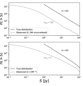
Figure 7: The effect of intra-channel dispersion smearing on the observed source counts slope. Plotted are the cumulative FRB brightness distributions for two simulated datasets: One in which DM and flux density are not correlated (top panel) and one in which DM is a distance measure, effecting an inverse square relation between brightness and dispersion (bottom panel). In both cases many events fall below the detection threshold due to smearing, but in the latter case the apparent source counts slope is significantly flattened due to the correlation between brightness and DM.

4.1.1 DM / brightness and $\log N$–$\log S$

There are a number of possible sources of covariance between DM and brightness. These include local phenomena, such as free-free absorption in a dense, dispersive plasma environment; cosmological effects like the redshifting of the emission spectrum into the observing bandpass; and variation in the source population with redshift.

If DM and brightness are correlated, then the observed source counts of FRBs can be altered by intra-channel dispersion smearing. For most, but not all, plausible luminosity functions, a cosmological population of FRBs will show an anti-correlation between fluence and extragalactic DM because dispersion is a proxy for distance in those cases (Niino, 2018); there may already be evidence for this in the data (Shannon et al., 2018). If flux density or fluence do scale inversely with DM, the smearing effects described in this paper will result in an apparent flattening of the brightness distribution. This is because high-DM events, which are also the dimmest in that scenario, are more susceptible to dispersion smearing and a greater fraction of them will fall below the detection threshold. This results in a relative abundance of bright FRBs and smaller measured values of $\alpha$. I demonstrate the effect of smearing on source counts in the presence of a brightness/DM_ex correlation in Fig. 7. In the simulation $2\times 10^{5}$ FRBs are generated with a Euclidean flux distribution such that, $n(s)\propto s^{-3/2}$. Their DMs are Gaussian with mean 1000 pc cm^-3 and standard deviation 500 pc cm^-3 as before, and pulse widths are lognormal. Intra-channel dispersion smearing is dominant over sampling time. Brightness and DM are either uncorrelated (top panel) or perfectly correlated (bottom panel), with DM $\propto 1/\sqrt{s}$. In the correlated case, the logarithmic source counts are flattened and the measured power-law index is lower than the input Euclidean value. The effect is more pronounced for larger values of $\alpha$ since a steep brightness distribution means more events are clustered around the S/N threshold.

4.1.2 DM / pulse width

DM and observed pulse width are trivially correlated, due to dispersion smearing. Extragalactic DM and intrinsic pulse width (as they arrive at our receivers) may also be correlated. One source of this is cosmological time dilation if DM scales with distance, since

$$t_{i}=t_{e}\,(1+z)\propto\,\mathrm{DM}_{\mathrm{ex}}.$$ (28)

Another potential source of this correlation is if there were a DM-scattering relationship analogous to that of Galactic pulsars (Bhat et al., 2004). This could arise if FRBs typically lived in dense ionic environments, where local electrons contributed a significant fraction of the source’s extragalactic dispersion. Such dense plasma environments are more likely to have a scattering screen along the FRB’s line-of-sight. In the framework of this paper, scattering alters only $n(t_{i})$ because I consider the intrinsic pulse width to be the burst duration as it arrives at our receivers. Regardless of the cause, if DM_ex and $t_{i}$ do indeed vary positively with one another due to cosmological or propagation broadening, higher-DM events will be more difficult to detect. This is because in those cases fluence is conserved, but detection S/N is not.

Similar to the proposed DM-brightness relation in ASKAP/Parkes sources, there may also be weak evidence for the aforementioned DM-scattering relationship: 7 of the 13 CHIME bursts found during pre-commissioning show temporal scattering and they report a weak correlation between scattering time and DM (CHIME/FRB Collaboration et al., 2019a). Ravi (2019) found weak evidence for this at 1400 MHz as well. Since the IGM itself is not expected to produce detectable temporal scattering (see, e.g., Luan & Goldreich (2014)), the DM_ex-scattering and DM_ex-brightness trends may appear to be at odds, at least superficially.

If these two results gain statistical significance and are found not to be selection effects, there are three ways to reconcile them. One explanation is that CHIME is probing a different population of FRBs at 600 MHz than is being probed at 1400 MHz. Alternatively, FRBs could be significantly dispersed by both the IGM and the local environment. Indeed, the one source whose local environment has been examined closely, FRB121102, appears to have roughly half of its extragalactic dispersion in the IGM and half in its host galaxy (Tendulkar et al., 2017; Michilli et al., 2018). A third explanation is that FRBs are dispersed by the IGM and scattered by the circumgalactic medium (CGM) of intervening galaxies (Vedantham & Phinney, 2019). Scattering timescale increases with distance to the screen, which is maximised when the screen is halfway between the observer and the source. Therefore, if the scattering of distant FRBs is dominated by screens in CGM halfway to the source, there ought to be a positive DM_ex-scattering correlation. A counterexample may be FRB110523: Masui et al. (2015) argued that its temporal scattering was due to a nearby screen, based on an angular broadening upper limit set by the fact that FRB110523 scintillates in our Galaxy; if that source were first scattered in the CGM of an intervening galaxy, its angular broadening would be large enough that it would no longer be a point source when arriving in the Milky Way.

4.1.3 Pulse width / brightness

Brightness and pulse width could be inversely related if width increased with distance, whether due to cosmological time dilation or DM smearing. There could also exist a correlation between brightness and pulse width in the presence of scattering, which broadens the pulse and decreases peak flux density. Depending on the relationship between the pulse luminosity distribution and the pulse energy distribution, the correlation may also be intrinsic. As a trivial example, if the total energy emitted in a pulse is roughly constant (called a “standard battery” by Macquart & Ekers (2018b)) rather than the total luminosity (“standard candle”), then pulse width and peak flux density would anti-correlate.

4.2 Giant pulses

Galactic pulsars emit single pulses with widths that span $\sim$ 9 orders-of-magnitude, the shortest of which are giant pulses (GPs). By analogy, if a blind survey were to search for GPs in our own Galaxy with current FRB back-ends, most would be missed due to smearing, as they typically have widths $<<$ ms. The Crab, for example, whose GPs have the highest brightness temperature of anything in the Universe ($\sim$ $10^{41}$ K), emits pulses that are $\sim$ microsecond at 1.4 GHz. No lower limit has been placed on its minimum pulse width, but Hankins et al. (2003) found Crab “nanoshots” of duration $<2$ ns. Similarly, the distribution of B1937+21’s GP widths was found to peak at 350 ns (McKee et al., 2018). If ASKAP were to search for a 1 $\mu$s Crab GP, its S/N would be reduced by a factor of 36 due to sampling smearing alone. Therefore, if FRBs also come from young neutron stars (Connor et al., 2016a; Cordes & Wasserman, 2016), and are similar to giant pulses from pulsars, the majority may be significantly narrower than 1 ms.

4.3 Low-frequency surveys

Blind FRB searches at frequencies below 200 MHz have been limited by the volume of parameter space they could search, primarily due to instrumental smearing (Coenen et al., 2014; Tingay et al., 2015; Rowlinson et al., 2016). As an example, for a real-time survey on LOFAR at 145 MHz, Karastergiou et al. (2015) used DM${}_{max}=320$ pc cm^-3 to avoid dispersion smearing. For many cosmological FRB scenarios, this could preclude detecting $\geq 90\%$ of FRBs. Even in the most optimistic case in Fig. 4, where there are few high-DM FRBs and they are all relatively broad, MWA’s current back-end allows for just $1\%$ of events would be recovered. The most recent results from LOFAR’s Fast Radio Transient Search (FRATS) was limited to DMs less than 500 pc cm^-3 (ter Veen et al., 2019). In this case, they were not limited by intra-channel or sampling smearing (the time and frequency resolution were 0.5 ms and 12 kHz respectively) but by the maximum dispersion delay across the band that could fit within their buffer boards.

Upper limits obtained from non-detections must be multiplied by the reciprocal of the survey’s completeness in width and DM, just as sky-coverage and brightness incompleteness are accounted for when constraints are made using beam size and a minimum detectable flux density. Width and DM completeness are difficult to know precisely, because computing them requires knowing the underlying distributions of FRBs. But there exist similar problems with beam size and brightness, and given the extent of incompleteness due to instrumental smearing in many cases, previous constraints at low frequencies could be significantly weakened when considering smearing.

Upcoming surveys will observe simultaneously at multiple frequencies. MWA has already successfully shadowed and recorded data at 185 MHz during three of ASKAP’s 1.4 GHz detections (Sokolowski et al., 2018). Nothing was found, allowing them to constrain the spectral index of those bursts over a decade in frequency. However, their 1.28 MHz frequency channels and 500 ms sampling time result in smearing, which would reduce a millisecond burst with a moderate DM by a factor of $\sim$30 in S/N. The Apertif LOFAR Exploration of the Radio Transient Sky (ALERT) will detect FRBs with Apertif at 1.4 GHz and trigger LOFAR at 150 MHz. This system has the advantage of recording voltage data, and will save 5 s of data in each frequency sub-band of LOFAR in order to extract the pulse’s dispersion sweep. For this reason, ALERT will be able to probe low-frequency FRB emission in an unprecedented way. The existence of temporally unresolved, unscattered FRBs detected down to the bottom of CHIME’s observing band at 400 MHz is promising for such programs (CHIME/FRB Collaboration et al., 2019a).

5 Conclusions

I have introduced a formalism for calculating FRB detection rates, and I have incorporated relevant burst and instrumental parameters that have previously been neglected. I have also presented a method for interpreting the distributions of FRB observables, focusing on DM, pulse width, and brightness. Depending on the intrinsic DM and pulse width distributions of FRBs, otherwise-similar telescopes can have orders-of-magnitude differences in detection rate depending on their time and frequency resolution, due only to the deleterious effects of temporal smearing (see, e.g., Fig 1). Perhaps more significantly, the interaction between the intrinsic distributions of FRB properties and the instruments that detect them can produce observed distributions that look very different from the inputs (Fig 3, Fig 6). I therefore caution against inferring physical properties about FRBs (luminosity function, spatial distribution, etc.) based on their observables without accounting for such selection effects, even when the analysis is done within a single survey.

I have argued that if there are substantial numbers of narrow FRBs, they would fall below our detection thresholds due to smearing. Based on the observed distributions of burst duration and the fact that coherently-dedispersed FRBs tend to show temporal structure at $<<$ ms, a population of microsecond-duration events may be likely. Another piece of evidence for the existence of narrow bursts comes from the 13 pre-commissioning CHIME FRBs (CHIME/FRB Collaboration et al., 2019a). By effectively fitting out frequency-dependent broadening effects like scattering and dispersion smearing, they found 4 events with duration $<500$ $\mu$s, even though that is well below their smearing timescale. Those events were detected despite attenuation due to smearing, but there are likely less bright events of similar widths did fall below the S/N threshold. The same arguments could be made about FRB150807, which was temporally unresolved at 350 $\mu$s and whose frequency spectrum implied structure at the level of several microseconds (Ravi et al., 2016).

To test the hypotheses that narrow or high-DM bursts are being missed, a Kolmogorov-Smirnov test could be run on current data from different telescopes, comparing the distribution of $t_{obs}/t_{sm}$ with those produced by simulated DM and width distributions. Another approach would be to alter the balance between time and frequency resolution on throughput-limited surveys in order to increase sensitivity in specific regions of width/DM space. For example, if FRBs are to be searched for at DM $>\,3000$ pc cm^-3, a survey could sacrifice time resolution or number of beams for increased channelization. A single telescope could carry out two distinct surveys with different time and frequency resolutions in order to investigate the underlying distributions of width and DM. To that end, I have presented a method for calculating the rate-optimized time and frequency resolution at a given survey was presented in Sect. 2.4.

Finally, I considered intrinsic correlations between various FRB parameters. I showed how dispersion smearing can lead to an apparent flattening of FRB source counts in the case where DM and brightness are inversely related. I also discussed the potential physical and instrumental causes for a positive correlation between DM and detected pulse width. As we enter an era in which multiple surveys will each have considerable collections of FRBs, the community will need end-to-end simulation pipelines that include instrumental selection effects and population synthesis (e.g. frbpoppy Gardenier et al. in prep (2019)). Still, due to the subtle selection effects involved in searching for and interpreting FRB detections, it is vital to understand such phenomena from the ground up.

References

- Amiri et al. (2017) Amiri M., et al., 2017, ApJ, 844, 161
- Bailes et al. (2017) Bailes M., et al., 2017, Publ. Astron. Soc. Australia, 34, e045
- Bannister et al. (2017) Bannister K. W., et al., 2017, ApJ, 841, L12
- Bhat et al. (2004) Bhat N. D. R., Cordes J. M., Camilo F., Nice D. J., Lorimer D. R., 2004, ApJ, 605, 759
- CHIME/FRB Collaboration et al. (2018) CHIME/FRB Collaboration et al., 2018, ApJ, 863, 48
- CHIME/FRB Collaboration et al. (2019a) CHIME/FRB Collaboration et al., 2019a, Nature, 566, 230
- CHIME/FRB Collaboration et al. (2019b) CHIME/FRB Collaboration et al., 2019b, Nature, 566, 235
- Caleb et al. (2016) Caleb M., Flynn C., Bailes M., Barr E. D., Hunstead R. W., Keane E. F., Ravi V., van Straten W., 2016, MNRAS, 458, 708
- Caleb et al. (2017) Caleb M., et al., 2017, MNRAS, 468, 3746
- Coenen et al. (2014) Coenen T., et al., 2014, A&A, 570, A60
- Connor et al. (2016a) Connor L., Sievers J., Pen U.-L., 2016a, MNRAS, 458, L19
- Connor et al. (2016b) Connor L., Lin H.-H., Masui K., Oppermann N., Pen U.-L., Peterson J. B., Roman A., Sievers J., 2016b, MNRAS, 460, 1054
- Cordes & McLaughlin (2003) Cordes J. M., McLaughlin M. A., 2003, ApJ, 596, 1142
- Cordes & Wasserman (2016) Cordes J. M., Wasserman I., 2016, MNRAS, 457, 232
- Farah et al. (2018) Farah W., et al., 2018, MNRAS, 478, 1209
- Gajjar et al. (2018) Gajjar V., et al., 2018, ApJ, 863, 2
- Hankins et al. (2003) Hankins T. H., Kern J. S., Weatherall J. C., Eilek J. A., 2003, Nature, 422, 141
- James et al. (2019) James C. W., et al., 2019, Publ. Astron. Soc. Australia, 36, e009
- Karastergiou et al. (2015) Karastergiou A., et al., 2015, MNRAS, 452, 1254
- Keane & Petroff (2015) Keane E. F., Petroff E., 2015, MNRAS, 447, 2852
- Lawrence et al. (2017) Lawrence E., Vander Wiel S., Law C., Burke Spolaor S., Bower G. C., 2017, AJ, 154, 117
- Lorimer et al. (2007) Lorimer D. R., Bailes M., McLaughlin M. A., Narkevic D. J., Crawford F., 2007, Science, 318, 777
- Luan & Goldreich (2014) Luan J., Goldreich P., 2014, ApJ, 785, L26
- Macquart & Ekers (2018a) Macquart J.-P., Ekers R. D., 2018a, MNRAS, 474, 1900
- Macquart & Ekers (2018b) Macquart J.-P., Ekers R., 2018b, MNRAS, 480, 4211
- Madau & Dickinson (2014) Madau P., Dickinson M., 2014, ARA&A, 52, 415
- Madhavacheril et al. (2019) Madhavacheril M. S., Battaglia N., Smith K. M., Sievers J. L., 2019, arXiv e-prints,
- Masui & Sigurdson (2015) Masui K. W., Sigurdson K., 2015, Physical Review Letters, 115, 121301
- Masui et al. (2015) Masui K., et al., 2015, Nature, 528, 523
- McKee et al. (2018) McKee J. W., et al., 2018, MNRAS,
- McQuinn (2014) McQuinn M., 2014, ApJ, 780, L33
- Michilli et al. (2018) Michilli D., et al., 2018, Nature, 553, 182
- Niino (2018) Niino Y., 2018, ApJ, 858, 4
- Oppermann et al. (2016) Oppermann N., Connor L. D., Pen U.-L., 2016, MNRAS, 461, 984
- Petroff et al. (2016) Petroff E., et al., 2016, Publ. Astron. Soc. Australia, 33, e045
- Ravi (2019) Ravi V., 2019, MNRAS, 482, 1966
- Ravi et al. (2016) Ravi V., et al., 2016, Science, 354, 1249
- Rowlinson et al. (2016) Rowlinson A., et al., 2016, MNRAS, 458, 3506
- Sanidas et al. (2017) Sanidas S., Caleb M., Driessen L., Morello V., Rajwade K., Stappers B. W., 2017, Proceedings of the International Astronomical Union, 13, 406–407
- Shannon et al. (2018) Shannon R. M., et al., 2018, Nature, 562, 386
- Sokolowski et al. (2018) Sokolowski M., et al., 2018, ApJ, 867, L12
- Spitler et al. (2014) Spitler L. G., et al., 2014, ApJ, 790, 101
- Spitler et al. (2016) Spitler L. G., et al., 2016, Nature, 531, 202
- Tendulkar et al. (2017) Tendulkar S. P., et al., 2017, ApJ, 834, L7
- Thornton et al. (2013) Thornton D., et al., 2013, Science, 341, 53
- Tingay et al. (2015) Tingay S. J., et al., 2015, AJ, 150, 199
- Vedantham & Phinney (2019) Vedantham H. K., Phinney E. S., 2019, MNRAS, 483, 971
- Vedantham et al. (2016) Vedantham H. K., Ravi V., Hallinan G., Shannon R. M., 2016, ApJ, 830, 75
- ter Veen et al. (2019) ter Veen S., et al., 2019, A&A, 621, A57
- van Leeuwen (2014) van Leeuwen J., 2014, in Wozniak P. R., Graham M. J., Mahabal A. A., Seaman R., eds, The Third Hot-wiring the Transient Universe Workshop. pp 79–79