Analysis of Metastable Behavior via Solutions of Poisson Equations

Abstract.

We herein review the recent progress on the study of metastability based on the analysis of solutions of Poisson equations related to the generators of the underlying metastable dynamics. This review paper is based on the joint work with Claudio Landim [24] and Fraydoun Rezakhanlou [26].

Acknowledgement.

This article is written as a proceeding to the 17th International Symposium Stochastic Analysis on Large Scale Interacting Systems held in the Research Institute for Mathematical Sciences (RIMS), Kyoto University from November 5–8, 2018. The author would like to thank the organizers for the invitation to the conference and the kind support during the stay. The author also thanks Professor Kenkichi Tsunoda for the invitation to Osaka University before the conference was held, during which most of the current article was written.

The author is deeply indebted to Professor Claudio Landim, who introduced the metastability theory to the author and shared numerous valuable ideas, and to Professor Fraydoun Rezakhanlou who first envisioned the approach explained herein and shared it with the author.

This work is supported by the National Research Foundation of Korea (NRF), grant funded by the Korea government (MSIT) (No. 2018R1C1B6006896 and No. 2017R1A5A1015626).

1. Quantitative Analysis of Metastable Behavior

Metastable behavior is a ubiquitous phenomenon exhibited by random dynamics in a low-temperature regime. To concretely describe this behavior, we first introduce a classic model known as the small random perturbation of dynamical systems (SRPDS, see [13] for an extensive discussion). For a smooth potential function $U:\mathbb{R}^{d}\rightarrow\mathbb{R}$ and small parameter $\epsilon>0$, we consider a stochastic differential equation given by

$$d\boldsymbol{y}_{\epsilon}(t)=-\nabla U(\boldsymbol{y}_{\epsilon}(t))dt+\sqrt{2\epsilon}\,d\boldsymbol{w}_{t}\;;\;t\geq 0\;,$$ (1.1)

where $(\boldsymbol{w}_{t})_{t\geq 0}$ represents the standard $d$-dimensional Brownian motion. If $U$ has several local minima as in Figure 1.1, the stochastic process $(\boldsymbol{y}_{\epsilon}(t))_{t\geq 0}$ exhibits the metastable behavior. To describe this behavior, we consider the zero-temperature dynamics described by the following ordinary differential equation:

$$d\boldsymbol{y}(t)=-\nabla U(\boldsymbol{y}(t))dt\;\;;\;t\geq 0\;.$$ (1.2)

Then, we can observe that the local minima of the potential function $U$ is the stable equilibria of the dynamics $(\boldsymbol{y}(t))_{t\geq 0}$. Namely, the dynamics starting at a domain of attraction of a local minimum $\boldsymbol{m}_{1}$ of $U$ converges to $\boldsymbol{m}_{1}$ exponentially fast. We can regard (1.1) as a small random perturbation of the deterministic dynamical system (1.2), provided that $\epsilon>0$ is small enough; hence, one can expect a similar behavior; the random process $(\boldsymbol{y}_{\epsilon}(t))_{t\geq 0}$ starting at a neighborhood of the local minimum $\boldsymbol{m}_{1}$ of $U$ will converge to $\boldsymbol{m}_{1}$.

Figure 1.1. Example of potential functions: (Left) Double-well potential, (Right) General potential with several global minima

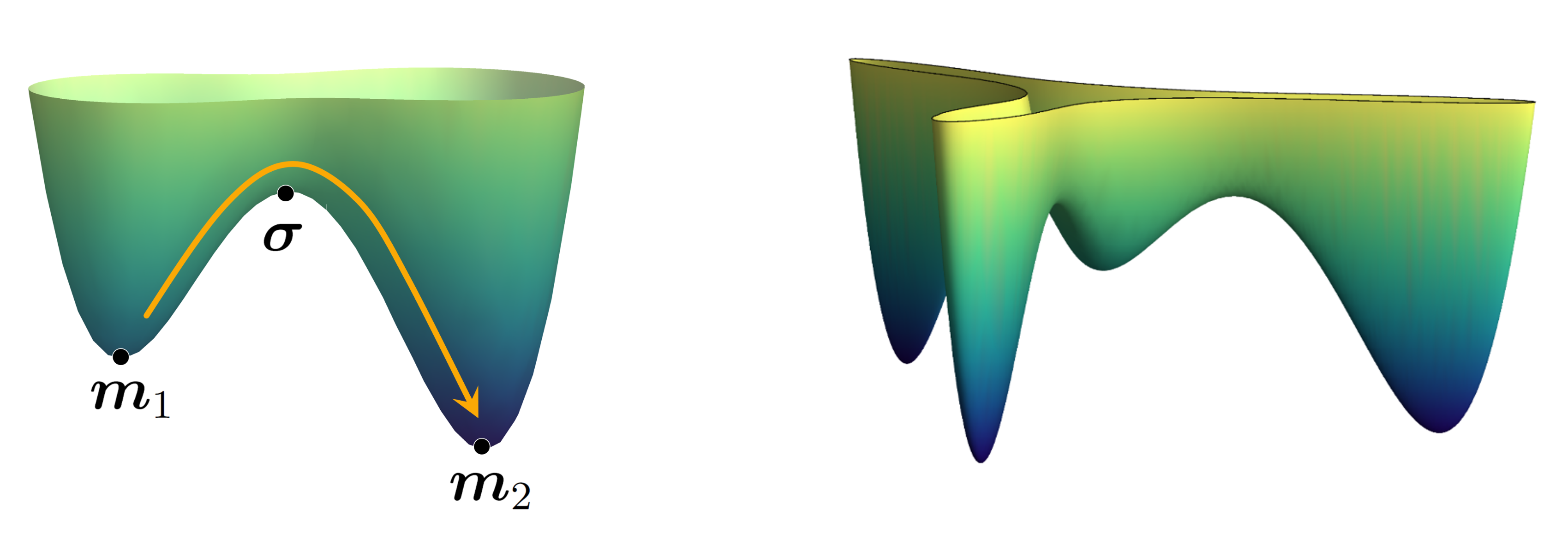
This estimates is locally true; however, if we consider the global picture, a crucial difference arises because of the randomness induced by the Brownian motion: if we wait for a sufficiently long time, then the process will move from the neighborhood of $\boldsymbol{m}_{1}$ to that of another local minimum, e.g., $\boldsymbol{m}_{2}$ (see Figure 1.1-(Right)). We now call the neighborhoods of each local minimum as the metastable set, and the transitions among these sets explained above are called the metastable transition. We expect that this metastable transition occurs repeatedly in a suitable time scale, and is an example of metastable behavior. This type of behavior is exhibited by numerous models, e.g., interacting particle systems such as the zero-range processes [1, 4, 18, 27], simple inclusion processes [6, 16], and ferromagnetic systems such as the Curie–Weiss model [5], Ising model [11] and, Potts model [23, 25].

To explain the primary questions in this study, we only focus on the SRPDS (1.1) in this introductory section. In the SRPDS, we can consider two cases as below, and the primary concerns are slightly different for each case.

• Case 1: $U$ contains several local minima but only one global minimum as in Figure 1.1-(Left). In this case, the process starting from any point first stabilizes at a neighborhood of the local minima. Subsequently, after a sufficiently long time, it performs a metastable transition toward the neighborhood of the global minimum, and remains therein for a longer time scale than the metastable transition time. Therefore, a primary object to be investigated is this metastable transition time from a local minimum to the global minimum. For instance, its expected value and asymptotic law are the primary concern. The robust methodology answering this question in a quantitative manner is the potential-theoretic approach developed by Bovier et al. in [7, 8]. This methodology is explained in Section 2.1.

• Case 2: $U$ contains multiple global minima as in Figure 1.1-(Right). As explained previously, a process starting from a neighborhood of a minimum will be stabilized in this set. However, after a sufficiently long time, we observed the metastable transition, and expect that this transition occurs repeatedly. Therefore, describing such hopping dynamics in a rigorous manner is an important problem from the mathematical perspective. In particular, one expects to demonstrate that a scaling limit of this process converges to a Markov chain among the metastable sets, in a suitable sense. In particular, if the underlying metastable dynamics is a Markov process on a finite set, a robust methodology for proving this scaling limit, which is called martingale approach, has been established by Beltran and Landim in [2, 3]. We explain this approach in Section 2.2.

Our new methodology introduced in Section 3 can be regarded as another approach to analyze Case 2, and provides concrete answers for some questions that cannot be answered by both of the approaches explained previously. In particular, we can conduct a rigorous analysis explained in Case 2, when the underlying dynamics is a diffusion process that is not a process on a finite set. We refer to [24, 26] for details. In this review paper, instead of focusing on this specific model, we attempt to deliver our general idea on this new approach by skipping the technical details. In Section 2, we review the previous approaches; in Section 3, we explain our alternative approach.

2. Review on Previous Approaches

We shall consider a family of Markov processes $\{(\boldsymbol{x}_{\epsilon}(t))_{t\geq 0}:\epsilon>0\}$ on $\Omega$. The sets $\mathcal{E}_{1},\,\ldots,\,\mathcal{E}_{K}$ represent the metastable set, i.e., the process $\boldsymbol{x}_{\epsilon}(t)$ starting from a point in a set $\mathcal{E}_{i}$ remains in this set sufficiently long when $\epsilon$ is small enough. Subsequently, after a sufficiently long time, the process exhibits a transition to another metastable set. We write $S=\{1,\,2,\,\ldots,\,K\}$ and let $\mu_{\epsilon}$ be the invariant measure of the process $\boldsymbol{x}_{\epsilon}(t)$. We denote by $\mathbb{P}_{\boldsymbol{x}}^{\epsilon}$ the law of process $\boldsymbol{x}_{\epsilon}(t)$ starting from $\boldsymbol{x}\in\Omega$, and denote by $\mathbb{E}_{\boldsymbol{x}}^{\epsilon}$ the corresponding expectation.

Remark 2.1.

The sets $\Omega$ and $\mathcal{E}_{1},\,\ldots,\,\mathcal{E}_{K}$ may depend on $\epsilon$. Instead of the family of Markov processes parameterized by $\epsilon$, one can consider the sequence of Markov processes $\{(\boldsymbol{x}_{N}(t))_{t\geq 0}:N\in\mathbb{N}\}$. The approaches explained below can be applied to this sequence as well. Instead of the $\epsilon\downarrow 0$ limit, we should consider the $N\uparrow\infty$ limit in this case.

2.1. Potential-theoretic approach

We first consider the question suggested in Case 1 of Section 1, namely, the estimation of the metastable transition time from a metastable set to others. To formulate this question concretely, we first introduce some notations. For $\mathcal{A}\subset\Omega$, we denote by $\tau_{\mathcal{A}}$ the hitting time of the set $\mathcal{A}$. We write $\mathcal{E}:=\bigcup_{i\in S}\mathcal{E}_{i}$ and $\breve{\mathcal{E}}_{i}=\mathcal{E}\setminus\mathcal{E}_{i}$. We pick a point $\boldsymbol{x}_{i}\in\mathcal{E}_{i}$ arbitrarily. Subsequently, the primary concern is the estimation of the mean transition time $\mathbb{E}_{\boldsymbol{x}_{i}}[\tau_{\breve{\mathcal{E}}_{i}}]$. This quantity corresponds to the escape time from a local minimum, and is crucially related to the mixing time and the spectral gap (see [10]).

It has been observed in [8] that, if the process $\boldsymbol{x}_{\epsilon}(t)$ is reversible with respect to the invariant measure $\mu_{\epsilon}$, then the mean transition time is closely related to a potential theoretic notion known as the capacity. For disjoint subsets $\mathcal{A}$ and $\mathcal{B}$ of $\Omega$, the equilibrium potential between $\mathcal{A}$ and $\mathcal{B}$ with respect to the process $\boldsymbol{x}_{\epsilon}(t)$ is a function $h_{\mathcal{A},\,\mathcal{B}}^{\epsilon}:\Omega\rightarrow[0,\,1]$ defined by

$$h_{\mathcal{A},\,\mathcal{B}}^{\epsilon}(\boldsymbol{x})=\mathbb{P}_{\boldsymbol{x}}^{\epsilon}\left[\tau_{\mathcal{A}}<\tau_{\mathcal{B}}\right]\;.$$

Subsequently, the capacity between $\mathcal{A}$ and $\mathcal{B}$ is defined by

$$\textup{cap}_{\epsilon}(\mathcal{A},\,\mathcal{B})=\int_{\Omega}h_{\mathcal{A},\,\mathcal{B}}^{\epsilon}(-\mathcal{L}_{\epsilon}h_{\mathcal{A},\,\mathcal{B}}^{\epsilon})d\mu_{\epsilon}\;,$$

where $\mathcal{L}_{\epsilon}$ is the generator corresponding to the process $\boldsymbol{x}_{\epsilon}(t)$. The crucial observation is that, under the circumstances of metastability, the following holds:

$$\mathbb{E}_{\boldsymbol{x}_{i}}[\tau_{\breve{\mathcal{E}}_{i}}]\simeq\frac{\mu_{\epsilon}(\mathcal{E}_{i})}{\textup{cap}_{\epsilon}(\mathcal{E}_{i},\,\breve{\mathcal{E}}_{i})}\;.$$ (2.1)

The asymptotic limit of $\mu_{\epsilon}(\mathcal{E}_{i})$ of $\epsilon\downarrow 0$ is typically not difficult to obtain. The non-trivial part is to estimate the capacity $\textup{cap}_{\epsilon}(\mathcal{E}_{i},\,\breve{\mathcal{E}}_{i})$. If the process $\boldsymbol{x}_{\epsilon}(t)$ is reversible with respect to $\mu_{\epsilon}$, it can be performed via the Dirichlet and Thomson principles that provide the upper and lower bounds for the capacity, respectively.

A successful application of this methodology is the Eyring-Kramers formula for the SRPDS (1.1). For this model, $\mathcal{E}_{i}$ can be regarded as a small $O(1)$ neighborhood (or $O(\epsilon^{1/2+\alpha})$, $\alpha>0$, neighborhood) of each local minimum. To deliver the primary result in a concrete and simple form, let us temporarily assume that $U$ is a double-well potential as in Figure 1.1-(Left): two local minima $\boldsymbol{m}_{1}$ and $\boldsymbol{m}_{2}$ exist, and a saddle point $\boldsymbol{\sigma}$ exists between them. The main result of [8] shows that, if the Hessians $\nabla^{2}U$ at $\boldsymbol{m}_{1},\,\boldsymbol{m}_{2},$ and $\boldsymbol{\sigma}$ are non-degenerate, and if $(\nabla^{2}U)(\boldsymbol{\sigma})$ has a unique negative eigenvalue $-\lambda_{\boldsymbol{\sigma}}$, then under some minor technical assumptions, the following holds:

$$\mathbb{E}_{\boldsymbol{m}_{1}}^{\epsilon}[\tau_{\mathcal{E}_{2}}]\,\text{$\simeq$}\,\frac{2\pi}{\lambda_{\sigma}}\,\sqrt{\frac{-\det(\nabla^{2}U)(\boldsymbol{\sigma})}{\det(\nabla^{2}U)(\boldsymbol{m}_{1})}}\,\exp\left\{\frac{U(\boldsymbol{\sigma})-U(\boldsymbol{m}_{1})}{\epsilon}\right\}\;.$$ (2.2)

It has also been verified that the normalized mean transition time $\tau_{\mathcal{E}_{2}}/\mathbb{E}_{\boldsymbol{m}_{1}}^{\epsilon}[\tau_{\mathcal{E}_{2}}]$ converges to a mean $1$ exponential random variable as $\epsilon\downarrow 0$. We remark that, in a general $U$, a similar but slightly more complicated expression for the quantity of the form $\mathbb{E}_{\boldsymbol{m}_{1}}^{\epsilon}[\tau_{\breve{\mathcal{E}}_{1}}]$ can be obtained similarly

This approach is extremely robust for the reversible case, as demonstrated by numerous successful applications for a wide scope of models. Instead of enumerating these examples, we refer to the monograph [9] for the comprehensive discussions of this stream of studies.

A shortcoming of this original method is that its application is limited to the case when the process $\boldsymbol{x}_{\epsilon}(t)$ is reversible. Recently, studies of the non-reversible case has shown significant improvements. First, Beltran and Landim [2, 3] found a formula corresponding to (2.1) that holds without the reversibility assumption. This formula is fairly similar to (2.1), and hence the sharp estimation of capacity is required as well. This is another difficulty because the classical Dirichlet and Thomson principles hold only for the reversible case. However, recently, two variational principles generalizing these principles to the non-reversible case has been obtained. Gaudillière and Landim in [14] found a generalization of the Dirichlet principle, and Slowik in [29] found that of the Thomson principle. It was developed for the discrete Markov process setting, but had been generalized to the continuous diffusion setting in [20] as well. These principles are more difficult to use than the case of reversible counterparts, because they are double variational principles in complicated spaces. However, Landim in [18] used this principle creatively to investigate the metastable behavior of the non-reversible zero-range process. It was the first study that presented quantitative results in the study of the metastable behavior of non-reversible processes. More recently, a manual for using this package of new machinery has been developed in [22] by Landim and the author of this article. This manual has been used in [23], [27], and [20] to perform the quantitative analysis on metastability.

2.2. Martingale approach

Although the potential-theoretic approach of metastability is a strong method for analyzing the metastable random process, it cannot answer the question suggested in Case 2 of Section 1. More precisely, if there are multiple metastable sets of the same depth, we can expect that a properly defined rescaled process should behave like a Markov chain on these metastable sets, but the sharp asymptotics obtained by the potential-theoretic approach cannot deduce this type of result. In this subsection, we explain the martingale approach established by Beltran and Landim in [2, 3, 17]. To explain this approach, we start by introducing several notations.

All the notations defined above are maintained. Recall that there are $K$ metastable sets $\mathcal{E}_{1},\,\ldots,\,\mathcal{E}_{K}$ for the process $\boldsymbol{x}_{\epsilon}(t)$. We define $S=\{1,\,2,\,\ldots,\,K\}$. Now we shall define a so-called trace process of $\boldsymbol{x}_{\epsilon}(t)$ on $\mathcal{E}$. Stating heuristically, this is a process obtained from $\boldsymbol{x}_{\epsilon}(t)$ by turning off the clock when the process is not in $\mathcal{E}$. To define this object rigorously, we define the following:

$$T_{\epsilon}(t)=\int_{0}^{t}\mathbf{1}\{\boldsymbol{x}_{\epsilon}(s)\in\mathcal{E}\}\,ds\;\;;\;t\in[0,\,\infty)\;.$$

It measures the amount of time that the process $\boldsymbol{x}_{\epsilon}(\cdot)$ has spent on the set $\mathcal{E}$ up to time $t$. Subsequently, we define the generalized inverse of $T_{\epsilon}(\cdot)$ as

$$S_{\epsilon}(t)=\sup\left\{s:T_{\epsilon}(s)\leq t\right\}\;.$$ (2.3)

Finally, the trace process $(\overline{\boldsymbol{x}}_{\epsilon}(t))_{t\geq 0}$ is defined by

$$\overline{\boldsymbol{x}}_{\epsilon}(t)=\boldsymbol{x}_{\epsilon}(S_{\epsilon}(t))\;.$$

One can check that this process is a Markov process on $\mathcal{E}$, with possible long jumps along the boundary $\partial\mathcal{E}=\cup_{i\in S}\partial\mathcal{E}_{i}$. We denote by $\chi_{\mathcal{A}}:\Omega\rightarrow\{0,\,1\}$ the indicator function on $\mathcal{A}\subset\Omega$, and define the projection function $\Psi:\mathcal{E}\rightarrow\{1,\,2,\,\ldots,\,K\}$ as

$$\Psi(\boldsymbol{x})=\sum_{i=1}^{K}i\,\chi_{\mathcal{E}_{i}}(\boldsymbol{x})\;.$$

Finally, we define the projected process as $\mathbf{x}_{\epsilon}(t)=\Psi(\overline{\boldsymbol{x}}_{\epsilon}(t))$ which is a random process on $S$. With this package of notations, our primary question can be stated as follows.

Question.

Can we prove that a scaling limit of the process $(\mathbf{x}_{\epsilon}(t))_{t\geq 0}$ converges to a Markov chain $(\mathbf{x}(t))_{t\geq 0}$ on $S$?

To answer this question, it would be ideal if we can determine a priori prediction of the correct time scale $\theta_{\epsilon}$ and of the candidate for the limiting Markov chain $\mathbf{x}(t)$. We would like to stress that these can be inferred from the results for the mean transition time obtained by the potential-theoretic approach explained in the previous subsection.

We denote by $\mathbb{P}_{\pi}^{\epsilon}$ the law of the Markov process $\boldsymbol{x}_{\epsilon}(t)$ with a starting measure $\pi$ on $\Omega$, and by $\mathbf{Q}_{i}$ the law of Markov chain $\mathbf{x}(t)$ starting at $i\in\mathbf{S}$. Finally, we denote by $\mathbf{Q}_{\pi}^{\epsilon}$ the law of the rescaled projected process $\big{(}\mathbf{x}_{\epsilon}(\theta_{\epsilon}t)\big{)}_{t\geq 0}$ under $\mathbb{P}_{\pi}$. The main theorem can be formulated as follows:

Theorem 2.2.

Fix $i\in S$. For $\epsilon>0$, let $\pi_{\epsilon}$ be a probability measure on $\Omega$ concentrated on $\mathcal{E}_{i}$. Then, $\mathbf{Q}_{\pi_{\epsilon}}^{\epsilon}$ converges to $\mathbf{Q}_{i}$ as $\epsilon$ tends to $0$.

The martingale approach established by Beltran and Landim in [2, 3, 17] provides a robust methodology to prove this theorem, especially when the process $\boldsymbol{x}_{\epsilon}(t)$ is a Markov process on a discrete set. This approach reduces the proof of Theorem 2.2 to the estimates of the so-called mean-jump rate between valleys. To state this more precisely, denote by $\overline{r}_{\epsilon}:\mathcal{E}\times\mathcal{E}\rightarrow\mathbb{R}$ the jump rate of the trace process $\overline{\boldsymbol{x}}_{\epsilon}(t)$, which is a Markov process on $\mathcal{E}$. Subsequently, the mean-jump rate between two metastable sets $\mathcal{E}_{i}$ and $\mathcal{E}_{j}$ is defined as

$$\mathbf{r}_{\epsilon}(i,\,j)=\frac{1}{\mu_{\epsilon}(\mathcal{E}_{i})}\sum_{\boldsymbol{x}\in\mathcal{E}_{i},\,\boldsymbol{y}\in\mathcal{E}_{j}}\mu_{\epsilon}(\boldsymbol{x})\overline{r}_{\epsilon}(\boldsymbol{x},\,\boldsymbol{y})\;.$$ (2.4)

Denote by $\mathbf{r}:S\times S\rightarrow\mathbb{R}$ the jump rate of the Markov chain $(\mathbf{x}(t))_{t\geq 0}$. The main result of Beltran and Landim can be summarized as follows: up to several technical requirements, proving

$$\lim_{\epsilon\rightarrow 0}\theta_{\epsilon}\mathbf{r}_{\epsilon}(i,\,j)=\mathbf{r}(i,\,j)$$ (2.5)

is enough to demonstrate Theorem 2.2. Such an implication has been verified by relating several martingale problems creatively. Although the rate $\overline{r}_{\epsilon}$, i.e., the jump rate of the trace process, is not an easy notion to manage, Beltran and Landim observed that its weighted average $\mathbf{r}_{\epsilon}$ has a rather simple expression in terms of the potential-theoretic notions, such as the capacity. For instance, if the process $\boldsymbol{x}_{\epsilon}(t)$ is reversible, we have

$$\mathbf{r}_{\epsilon}(i,\,j)=\frac{1}{2}\left[\textup{cap}_{\epsilon}(\mathcal{E}_{i},\,\breve{\mathcal{E}}_{i})+\textup{cap}_{\epsilon}(\mathcal{E}_{j},\,\breve{\mathcal{E}}_{j})-\textup{cap}_{\epsilon}(\mathcal{E}_{i}\cup\mathcal{E}_{j},\,\breve{\mathcal{E}}_{i}\cap\breve{\mathcal{E}}_{j})\right]\;.$$ (2.6)

Thus, the analysis of metastable behavior can be performed by estimating the capacity, similar as before. This technology has been applied to various reversible models such as the zero-range process [4], the simple inclusion process [6], and random walks in a potential field [21].

Furthermore, the result of Beltran and Landim in [3] indicates that the implication from (2.5) to Theorem 2.2 also holds for the non-reversible case. The difficulty in the non-reversible case is that the formula (2.6) for $\mathbf{r}_{\epsilon}$ is no longer valid. Meanwhile, a rather complicated formula for $\mathbf{r}_{\epsilon}$ in terms of the so-called collapsed Markov chain has been found in [3] and [18]. Based on this, Landim in [18] first established an analysis of the non-reversible metastable process by analyzing the totally asymmetric zero-range process. Subseqeuntly, a robust way to use this complicated formula to deduce (2.5) is established in [22]. Recently, this has been applied to various non-reversible models in [22, 23, 27]. We refer to the review paper [19] by Landim for the comprehensive discussion of this topic.

Before concluding this review section, we have to emphasize that the martingale approach has not yet been successfully applied to metastable diffusion processes such as the SRPDS (1.1). Because in this case the trace process becomes a diffusion process on disconnected set $\mathcal{E}$ with a long jump along $\partial\mathcal{E}$, which is not a conventional object, the mean-jump rate such as (2.4) is almost impossible to define. Our new methodology (explained in the next section) can be regarded as an entirely different approach to metastability, and can be applied to continuous models such as the SRPDS that cannot be answered by the martingale approach.

3. Approach via Poisson Equations

We recall all the notations from the previous section. In this section, we explain a new approach developed in [24, 26]. This approach provides an alternative method to prove Theorem 2.2 by analyzing a Poisson equation, instead of estimating the potential-theoretic notions such as capacity.

We shall assume that we have predictions of correct time scale $\theta_{\epsilon}$ as well as the limiting Markov chain $\mathbf{x}(t)$, as mentioned before. In addition, we assume that

$$\mu_{\epsilon}(\mathcal{E}_{i})=(1+o_{\epsilon}(1))\,\nu(i)\;\;;\;\text{for all }i\in\{1,\,\dots,\,K\}\;,$$ (3.1)

where $\nu$ is a measure on $S=\{1,\,\cdots,\,K\}$ satisfying

$$\sum_{i=1}^{K}\nu(i)=1\;,$$ (3.2)

Therefore, using (3.1) and (3.2), we can verify that $\nu$ is the invariant measure of to the Markov chain $\mathbf{x}(t)$, provided that Theorem 2.2 is correct.

Denote by $\mathcal{L}_{\epsilon}$ and $\mathbf{L}$ the generators corresponding to the Markov processes $\boldsymbol{x}_{\epsilon}(t)$ and $\mathbf{x}(t)$, respectively. Define $\mathbf{a}_{\epsilon}=(\mathbf{a}_{\epsilon}(i):i\in S)\in\mathbb{R}^{S}$ by

$$\mathbf{a}_{\epsilon}(i)=\frac{\nu(i)}{\mu_{\epsilon}(\mathcal{E}_{i})}\;\;;\;i\in S\;.$$

By (3.1), we have

$$\mathbf{a}_{\epsilon}(i)=1+o_{\epsilon}(1)\text{ for all }i\in S\;.$$ (3.3)

The following proposition is the primary step in our new approach.

Proposition 3.1.

For all $\mathbf{f}:S\rightarrow\mathbb{R}$, there exists a bounded function $\phi_{\epsilon}=\phi_{\epsilon}^{\mathbf{f}}:\Omega\rightarrow\mathbb{R}$ satisfying the following conditions simultaneously:

1. The function $\phi_{\epsilon}$ satisfies the following equation:

   $$\mathcal{\mathscr{\mathcal{L}}_{\epsilon}}\phi_{\epsilon}=\theta_{\epsilon}^{-1}\sum_{i\in S}\mathbf{a}_{\epsilon}(i)\,(\mathbf{L}\mathbf{f})(i)\,\chi_{\mathcal{E}_{i}}\;.$$ (3.4)

2. For all $i\in S$, the following holds:

   $$\lim_{\epsilon\rightarrow 0}\sup_{x\in\mathcal{E}_{i}}\left|\phi_{\epsilon}(x)-\mathbf{f}(i)\right|=0\;.$$ (3.5)

We observed that finding a test function $\phi_{\epsilon}^{\mathbf{f}}$ explained in the last proposition implies Theorem 2.2, up to several minor technical issues. Hence, in the remaining part of the current section, we explain the model-independent proof of Theorem 2.2 assuming Proposition 3.1. The proof of Proposition 3.1 it the only model-dependent part. We explain a general idea for this part in Section 3.3.

In general, two ingredients are required to complete the proof of the limit theorem such as Theorem 2.2: the tightness of family $(\mathbf{Q}_{\pi_{\epsilon}}^{\epsilon})_{\epsilon>0}$, and the identification of limit points of this family. These two crucial ingredients are proven in Sections 3.1 and 3.2, respectively.

3.1. Tightness

For convenience, we fix $i\in S$ and the sequence of the family of probability measures $(\pi_{\epsilon})_{\epsilon>0}$ concentrated on $\mathcal{E}_{i}$ throughout this subsection. The tightness result required in our context can be stated as the following proposition.

Proposition 3.2.

The family $\{\mathbf{Q}_{\pi_{\epsilon}}^{\epsilon}:\epsilon\in(0,\,1]\}$ is tight on $D([0,\,\infty),\,S)$. Furthermore, every limit points $\mathbf{Q}^{*}$ of this family, as $\epsilon$ tends to $0$, satisfy

$$\mathbf{Q}^{*}(\mathbf{x}(0)=i)=1\text{\;\;and\;\;}\mathbf{Q}^{*}(\mathbf{x}(t)\neq\mathbf{x}(t-))=0\;\;\text{for all }t>0\;.$$

It is shown in [24, Sections 7, 8] that the proof of this tightness result is based entirely on the two estimates stated in Lemmas 3.3 and 3.4. The former verifies that a transition from a metastable set to another one cannot occur in a scale shorter than $\theta_{\epsilon}$, while the latter demonstrates that in the course of the metastable transition, the process does not spend much time outside the metastable sets, namely $\Omega\setminus\mathcal{E}$. We start by proving the former lemma, whose proof depends solely on Proposition 3.1. We simply write $\mathbb{P}_{\boldsymbol{x}}^{\epsilon}:=\mathbb{P}_{\delta_{\boldsymbol{x}}}^{\epsilon}$, where $\delta_{\boldsymbol{x}}$ is a Dirac delta measure at $\boldsymbol{x}\in\Omega$.

Lemma 3.3.

It holds that

$$\lim_{a\rightarrow 0}\limsup_{\epsilon\rightarrow 0}\sup_{\boldsymbol{x}\in\mathcal{E}_{i}}\mathbb{P}_{\boldsymbol{x}}^{\epsilon}\left[\tau_{\breve{\mathcal{E}}_{i}}\leq a\theta_{\epsilon}\right]=0\;.$$ (3.6)

Proof.

Consider a function $\mathbf{f}:S\rightarrow\mathbb{R}$ defined by

$$\mathbf{f}(j)=\begin{cases}0&\text{if }j=i\\ 1&\text{otherwise\;.}\end{cases}$$

Denote by $\phi_{\epsilon}=\phi_{\epsilon}^{\mathbf{f}}$ the function that we obtain in Proposition 3.1 with respect to this function $\mathbf{f}$. For $\boldsymbol{x}\in\mathcal{E}_{i}$, by Itö’s formula and (3.4), one can deduce that

$$\mathbb{E}_{\boldsymbol{x}}^{\epsilon}\left[\phi_{\epsilon}(\boldsymbol{x}_{\epsilon}(a\theta_{\epsilon}\wedge\tau_{\mathcal{E}\setminus\mathcal{E}_{i}}))\right]-\phi_{\epsilon}(\boldsymbol{x})$$

$$\quad=\sum_{i\in S}\mathbb{E}_{\boldsymbol{x}}^{\epsilon}\left[\int_{0}^{a\theta_{\epsilon}\wedge\tau_{\mathcal{E}\setminus\mathcal{E}_{i}}}\theta_{\epsilon}^{-1}\mathbf{a}_{\epsilon}(i)\,(\mathbf{L}\mathbf{f})(i)\,\chi_{\mathcal{E}_{i}}(\boldsymbol{x}_{\epsilon}(s))ds\right]\;.$$ (3.7)

It is noteworthy that for some constant $C>0$,

$$\left|\int_{0}^{a\theta_{\epsilon}\wedge\tau_{\mathcal{E}\setminus\mathcal{E}_{i}}}\theta_{\epsilon}^{-1}\mathbf{a}_{\epsilon}(i)\,(\mathbf{L}\mathbf{f})(i)\,\chi_{\mathcal{E}_{i}}(\boldsymbol{x}_{\epsilon}(s))ds\right|\leq a\theta_{\epsilon}\cdot\theta_{\epsilon}^{-1}|\mathbf{a}_{\epsilon}(i)\,(\mathbf{L}\mathbf{f})(i)|\leq Ca\;.$$ (3.8)

Moreover, since $\boldsymbol{x}\in\mathcal{E}_{i}$, it follows from (3.5) that

$$|\phi_{\epsilon}(\boldsymbol{x})|=|\phi_{\epsilon}(\boldsymbol{x})-\mathbf{f}(i)|=o_{\epsilon}(1)\;.$$ (3.9)

By combining (3.7), (3.8), and (3.9), we can deduce that

$$\mathbb{E}_{\boldsymbol{x}}^{\epsilon}\left[\phi_{\epsilon}(\boldsymbol{x}_{\epsilon}(a\theta_{\epsilon}\wedge\tau_{\mathcal{E}\setminus\mathcal{E}_{i}}))\right]\leq Ca+o_{\epsilon}(1)\;.$$ (3.10)

Next we attempt to bound the last expectation from below. Let $\delta>0$ be an arbitrarily small constant. Then, again by (3.5), we have $\phi_{\epsilon}+\delta\geq 0$ on $\mathcal{E}_{i}$ and $\phi_{\epsilon}+\delta\geq 1$ on $\mathcal{E}\setminus\mathcal{E}_{i}$ for all sufficiently small $\epsilon$. Hence, by the maximum principle, $\phi_{\epsilon}+\delta\geq 0$ on $\Omega$. Summing these, we have $\phi_{\epsilon}+\delta\geq\chi_{\mathcal{E}\setminus\mathcal{E}_{i}}$. Therefore,

$$\mathbb{E}_{\boldsymbol{x}}^{\epsilon}\left[\phi_{\epsilon}(\boldsymbol{x}_{\epsilon}(a\theta_{\epsilon}\wedge\tau_{\mathcal{E}\setminus\mathcal{E}_{i}}))+\delta\right]\geq\mathbb{E}_{\boldsymbol{x}}^{\epsilon}\left[\chi_{\mathcal{E}\setminus\mathcal{E}_{i}}(\boldsymbol{x}_{\epsilon}(a\theta_{\epsilon}\wedge\tau_{\mathcal{E}\setminus\mathcal{E}_{i}}))\right]=\mathbb{P}_{\boldsymbol{x}}^{\epsilon}\left[\tau_{\mathcal{E}\setminus\mathcal{E}_{i}}<a\theta_{\epsilon}\right]\;.$$ (3.11)

By (3.10) and (3.11), we deduce

$$\limsup_{\epsilon\rightarrow 0}\sup_{\boldsymbol{x}\in\mathcal{E}_{i}}\mathbb{P}_{\boldsymbol{x}}^{\epsilon}\left[\tau_{\mathcal{E}\setminus\mathcal{E}_{i}}\leq a\theta_{\epsilon}\right]\leq Ca+\delta$$

Because $\delta>0$ is arbitrary, the proof is completed. ∎

Next, we discuss the second ingredient. Denote by $\Delta=\Omega\setminus\mathcal{E}$ the outside of the metastable sets. Subsequently, by (3.1) and (3.2), we have $\mu_{\epsilon}(\Delta)=o_{\epsilon}(1)$. In other words, the set $\Delta$ is negligible in view of the equilibrium measure. However, the second ingredient of tightness requires us to show this negligibility of $\Delta$ in a dynamical sense. Hence, we define the excursion time of the process $\boldsymbol{x}_{\epsilon}(t)$ on the set $\Delta$ up to time $t$ as

$$\Delta(t)=\int_{0}^{t}\chi_{\Delta}(\boldsymbol{x}_{\epsilon}(s))\,ds\;.$$

We remark that $\Delta(t)$ is a notion depending on $\epsilon$ although we did not stress this in the notation. Then, we can formulate the dynamic negligibility of $\Delta$ as follows:

Lemma 3.4.

For any sequence $(\pi_{\epsilon})_{\epsilon>0}$ of probability measures concentrated on $\mathcal{E}_{i}$, the following holds:

$$\lim_{\epsilon\rightarrow 0}\theta_{\epsilon}^{-1}\mathbb{E}_{\pi_{\epsilon}}^{\epsilon}\left[\Delta(\theta_{\epsilon}t)\right]=0\;\;\text{for all }t\geq 0.$$

Here, we only provide the proof of Lemma 3.4 when $\pi_{\epsilon}$ has a density function with respect to $\mu_{\epsilon}$ for each $\epsilon>0$, and this density function belongs to $L^{p}(\mu_{\epsilon})$ for some $p>1$ in a uniform manner, i.e.,

$$\limsup_{\epsilon\rightarrow 0}\int_{\Omega}\left|\frac{d\pi_{\epsilon}}{d\mu_{\epsilon}}\right|^{p}d\mu_{\epsilon}=M<\infty.$$ (3.12)

For this case with mild initial distribution, we can deduce a simple proof. For the general case, see the remark after the proof.

Proof of Lemma 3.4 under the assumption (3.12).

We fix $t\geq 0$ and write

$$u_{\epsilon}(\boldsymbol{x})=\theta_{\epsilon}^{-1}\mathbb{E}_{\boldsymbol{x}}^{\epsilon}\left[\Delta(\theta_{\epsilon}t)\right]\;.$$

By Fubini’s theorem, we obtain

$$\int_{\Omega}u_{\epsilon}\,d\mu_{\epsilon}=\theta_{\epsilon}^{-1}\mathbb{E}_{\mu_{\epsilon}}^{\epsilon}\left[\int_{0}^{\theta_{\epsilon}t}\chi_{\Delta}(\boldsymbol{x}_{\epsilon}(s))ds\right]=\theta_{\epsilon}^{-1}\int_{0}^{\theta_{\epsilon}t}\mathbb{P}_{\mu_{\epsilon}}^{\epsilon}\left[\boldsymbol{x}_{\epsilon}(s)\in\Delta\right]ds=t\,\mu_{\epsilon}(\Delta)\;.$$ (3.13)

We write $f_{\epsilon}=\frac{d\pi_{\epsilon}}{d\mu_{\epsilon}}$ so that we can write

$$\theta_{\epsilon}^{-1}\mathbb{E}_{\pi_{\epsilon}}^{\epsilon}\left[\Delta(\theta_{\epsilon}t)\right]=\int_{\Omega}(u_{\epsilon}f_{\epsilon})\,d\mu_{\epsilon}$$ (3.14)

Now, we apply Holder’s inequality, trivial bound $u_{\epsilon}\leq t$, (3.13) and (3.12) to the right-hand side of the previous display to deduce the following:

$$\int_{\Omega}(u_{\epsilon}f_{\epsilon})\,d\mu_{\epsilon} \leq\left[\int_{\Omega}u_{\epsilon}\,d\mu_{\epsilon}\right]^{1/q}\left[\int_{\Omega}(u_{\epsilon}f_{\epsilon}^{p})\,d\mu_{\epsilon}\right]^{1/p}$$

$$\leq t\mu_{\epsilon}(\Delta)^{1/q}\,\left[\int_{\mathbb{R}^{d}}f_{\epsilon}^{p}\,d\mu_{\epsilon}\right]^{1/p}<t\mu_{\epsilon}(\Delta)^{1/q}M^{1/p}\;,$$ (3.15)

where $q$ is the conjugate exponent of $p$ satisfying $\frac{1}{p}+\frac{1}{q}=1$. Since $\mu_{\epsilon}(\Delta)=o_{\epsilon}(1)$, we complete the proof by conditions (3.14) and (3.15). ∎

Remark 3.5.

To address the general case, it is sufficient to demonstrate that

$$\lim_{\epsilon\rightarrow 0}\sup_{\boldsymbol{x}\in\mathcal{E}_{i}}\theta_{\epsilon}^{-1}\mathbb{E}_{\boldsymbol{x}}^{\epsilon}\left[\Delta(\theta_{\epsilon}t)\right]=0\;.$$

In view of the previous lemma for the special case, it suffices to verify that

$$\sup_{\boldsymbol{x},\,\boldsymbol{y}\in\mathcal{E}_{i}}\left(\mathbb{E}_{\boldsymbol{x}}^{\epsilon}\left[\Delta(\theta_{\epsilon}t)\right]-\mathbb{E}_{\boldsymbol{y}}^{\epsilon}\left[\Delta(\theta_{\epsilon}t)\right]\right)\ll\theta_{\epsilon}\;.$$

When $\Omega$ is a discrete set, this can be typically performed by the coupling (see [2, 3]). In the case of diffusion processes in a $1$-dimensional torus, the same type of coupling argument can be applied (see [24]). However, the diffusion processes such as the SRPDS (1.1) in dimension $d\geq 2$, two processes starting from different points cannot be coupled exactly; hence, another argument is required. In [26, Appendix], an argument based on the large-deviation theory has been introduced. We refer to these listed articles for the details of the proof of Lemma 3.4 for general cases.

The proof of Proposition 3.2 from these two lemmas above are routine and follows from Aldous’ criterion. We refer to [24, Section 7] or [26, Section 5] for more details, but we herein provide a brief sketch of the proof. First, we should introduce the appropriate filtration. Write $\widehat{\boldsymbol{x}}_{\epsilon}(t)=\boldsymbol{x}_{\epsilon}(\theta_{\epsilon}t)$ as the accelerated process, and write $\widehat{\mathbb{P}}_{\pi_{\epsilon}}^{\epsilon}$ the law of process $(\widehat{\boldsymbol{x}}_{\epsilon}(t))_{t\geq 0}$ starting from $\pi_{\epsilon}$. Then, denote by $\{\mathscr{F}_{t}^{0}:t\geq 0\}$ the natural filtration of $D([0,\,\infty),\,\Omega)$ (or $C([0,\,\infty),\,\Omega)$ if $(\boldsymbol{x}_{\epsilon}(t))$ is a diffusion process) with respect to the process $\widehat{\boldsymbol{x}}_{\epsilon}(\cdot)$, namely,

$$\mathscr{F}_{t}^{0}=\sigma(\widehat{\boldsymbol{x}}_{\epsilon}(s):s\in[0,\,t])\;.$$

and define $\{\mathscr{F}_{t}:t\geq 0\}$ as the usual augmentation of $\{\mathscr{F}_{t}^{0}:t\geq 0\}$ with respect to $\mathbb{\widehat{\mathbb{P}}}_{\pi_{\epsilon}}^{\epsilon}$ . Define $\mathscr{G}_{t}=\mathscr{F}_{S_{\epsilon}(t)}$ for $t\geq 0$, where $S_{\epsilon}$ is defined in (2.3). For $M>0$, we define $\mathcal{\mathscr{T}}_{M}$ as the collection of stopping times with respect to the filtration $\{\mathscr{G}_{t}\}_{t\geq 0}$ bounded by $M$.

Proof of Proposition 3.2.

We start by considering the first statement of the proposition. By Aldous’ criterion, it suffices to verify that, for all $M>0$,

$$\lim_{a_{0}\rightarrow 0}\limsup_{\epsilon\rightarrow 0}\sup_{\tau\in\mathcal{\mathscr{T}}_{M}}\sup_{a\in(0,\,a_{0})}\mathbb{P}_{\pi_{\epsilon}}^{\epsilon}\left[\mathbf{x}_{\epsilon}(\tau+a)\neq\mathbf{x}_{\epsilon}(\tau)\right]=0\;.$$ (3.16)

By Lemma 3.4, it suffices to demonstrate that

$$\lim_{a_{0}\rightarrow 0}\limsup_{\epsilon\rightarrow 0}\sup_{\tau\in\mathcal{\mathscr{T}}_{M}}\sup_{a\in(0,\,a_{0})}\mathbb{P}_{\pi_{\epsilon}}^{\epsilon}\left[\mathbf{x}_{\epsilon}(\tau+a)\neq\mathbf{x}_{\epsilon}(\tau),\,S_{\epsilon}(\tau+a)-S_{\epsilon}(\tau)\leq 2a_{0}\right]=0\;.$$

Since $\mathbf{x}_{\epsilon}(t)=\Psi(\widehat{\boldsymbol{x}}_{\epsilon}(S_{\epsilon}(t)))$, the last probability can be bounded above by

$$\mathbb{P}_{\pi_{\epsilon}}^{\epsilon}\left[\Psi(\widehat{\boldsymbol{x}}_{\epsilon}(S_{\epsilon}(\tau)+t)\neq\Psi(\widehat{\boldsymbol{x}}_{\epsilon}(S_{\epsilon}(\tau)))\;\text{for some }t\in(0,\,2a_{0}]\right]\;.$$

One can readily demonstrate that $S^{\epsilon}(\tau)$ is a stopping time with respect to the filtration $\{\mathscr{F}_{t}\}$ (see [24, Lemma 7.2]); hence, by the strong Markov property the last probability is bounded above by

$$\sup_{\boldsymbol{x}\in\mathcal{E}_{i}}\mathbb{P}_{\boldsymbol{x}}^{\epsilon}\left[\Psi(\widehat{\boldsymbol{x}}_{\epsilon}(t))\neq\Psi(\boldsymbol{x})\;\text{for some }t\in(0,\,2a_{0}]\right]=\sup_{\boldsymbol{x}\in\mathcal{E}_{i}}\mathbb{P}_{\boldsymbol{x}}^{\epsilon}\left[\tau_{\breve{\mathcal{E}}_{i}}\leq 2a_{0}\theta_{\epsilon}\right]\;.$$

Thus, the proof of (3.16) is completed by Lemma 3.3.

The assertion $\mathbf{Q}^{*}(\mathbf{x}(0)=i)=1$ is trivial. For the last assertion of the proposition, it suffices to prove that

$$\lim_{a_{0}\rightarrow 0}\limsup_{\epsilon\rightarrow 0}\mathbb{P}_{\pi_{\epsilon}}^{\epsilon}\left[\mathbf{x}_{\epsilon}(t-a)\neq\mathbf{x}_{\epsilon}(t)\text{ for some }a\in(0,\,a_{0})\right]=0\;.$$

The proof for this is the same as that above. ∎

3.2. Identification of limit points and the proof of Theorem 2.2

The proof of Theorem 2.2 can be completed by identifying the limit points of $(\mathbf{Q}_{\pi_{\epsilon}}^{\epsilon})_{\epsilon>0}$. To this end, fix $\mathbf{f}\in\mathbb{R}^{S}$, and let $\phi_{\epsilon}=\phi_{\epsilon}^{\mathbf{f}}$ be the function obtained in Proposition 3.1. We fix $i$ and $\pi_{\epsilon}$ appearing in the statement of Theorem 2.2. Since the generator of the accelerated process $\widehat{\boldsymbol{x}}(t)$ is $\theta_{\epsilon}\mathcal{L}_{\epsilon}$, the process $(M_{\epsilon}(t))_{t\geq 0}$ defined by

$$M_{\epsilon}(t)=\phi_{\epsilon}(\widehat{\boldsymbol{x}}_{\epsilon}(t))-\theta_{\epsilon}\int_{0}^{t}(\mathscr{\mathcal{L}}_{\epsilon}\phi_{\epsilon})(\widehat{\boldsymbol{x}}_{\epsilon}(s))ds$$

is a martingale with respect to the filtration $\{\mathscr{F}_{t}\}$ introduced above. Since $\widehat{\boldsymbol{x}}_{\epsilon}(S_{\epsilon}(t))=\boldsymbol{\overline{x}}_{\epsilon}(\theta_{\epsilon}t)$ by definition, we can write

$$M_{\epsilon}(S_{\epsilon}(t))=\phi_{\epsilon}(\boldsymbol{\overline{x}}_{\epsilon}(\theta_{\epsilon}t))-\theta_{\epsilon}\int_{0}^{t}(\mathscr{\mathcal{L}}_{\epsilon}\phi_{\epsilon})(\boldsymbol{\overline{x}}_{\epsilon}(\theta_{\epsilon}s))ds\;.$$ (3.17)

Since $\mathscr{G}_{t}=\mathscr{F}_{S_{\epsilon}(t)}$ (see [26, Lemma 5.5]), the process $(M_{\epsilon}(S_{\epsilon}(t)))_{t\geq 0}$ is a martingale with respect to $\{\mathscr{G}_{t}\}$. By Proposition 3.1, we have

$$\phi_{\epsilon}=\mathbf{f}\circ\Psi+o_{\epsilon}(1)\;\;\text{and\;\;}\mathscr{\theta_{\epsilon}\mathcal{L}}_{\epsilon}\phi_{\epsilon}=(\mathbf{L}\mathbf{f})\circ\Psi+o_{\epsilon}(1)\;\;\text{on }\mathcal{E}\;.$$

Since $\Psi(\boldsymbol{\overline{x}}_{\epsilon}(\theta_{\epsilon}t))=\mathbf{x}_{\epsilon}(t)$, we can rewrite (3.17) as

$$M_{\epsilon}(S_{\epsilon}(t))) =\mathbf{f}(\mathbf{x}_{\epsilon}(t))-\int_{0}^{t}(\mathbf{L}\mathbf{f})(\mathbf{x}_{\epsilon}(s))ds+o_{\epsilon}(1)\;.$$

Hence, if $\mathbf{Q}^{*}$ is a limit point of the family $\{\mathbf{Q}_{\pi_{\epsilon}}^{\epsilon}\}_{\epsilon\in(0,\,1]}$, the process $(M^{*}(t))_{t\geq 0}$ defined by

$$M^{*}(t)=\mathbf{f}(\mathbf{x}(t))-\int_{0}^{t}(\mathbf{L}\mathbf{f})(\mathbf{x}(s))ds$$ (3.18)

is a martingale under $\mathbf{Q}^{*}$. This completes the characterization of the limit points.

Proof of Theorem 2.2.

Let $\mathbf{Q}^{*}$ be a limit point of the family $\{\mathbf{Q}_{\pi_{\epsilon}}^{\epsilon}\}_{\epsilon\in(0,\,1]}$. Subsequently, as demonstrated above, $(M(t))_{t\geq 0}$ defined by (3.18) is a martingale under $\mathbf{Q}^{*}$; furthermore, by Proposition 3.2, we obtain $\mathbf{Q}^{*}[\mathbf{x}(0)=i]=1$ and $\mathbf{Q}^{*}(\mathbf{x}(t)\neq\mathbf{x}(t-))=0$ for all $t>0$. The only probability measure on $D([0,\,\infty),\,S)$ satisfying these properties simultaneously is $\mathbf{Q}_{i}$; thus, we can conclude that $\mathbf{Q}^{*}=\mathbf{Q}_{i}$. This completes the proof. ∎

3.3. Analysis of Poisson Equation

In view of the argument presented in the previous section, the entire analysis is dependent on the construction of $\phi_{\epsilon}^{\mathbf{f}}$ introduced in Proposition 3.1. This should be proven for each model.

For the non-reversible diffusion processes in a $1$-dimensional torus considered in [24], we found an explicit solution $\psi_{\epsilon}$ of the equation (3.4). It is noteworthy that for each constant $c_{\epsilon}$, the function $\psi_{\epsilon}+c_{\epsilon}$ is also a solution of (3.4). Hence, in this case we can select $c_{\epsilon}$ carefully such that the function $\phi_{\epsilon}=\psi_{\epsilon}+c_{\epsilon}$ satisfies (3.5) as well. We refer to [24, Section 9] for the details.

For the SRPDS (1.1) in $\mathbb{R}^{d}$, we cannot expect such a closed form solution. We shall sketch our idea of the proof in the next paragraph. We believe that the idea presented herein can be applied to a broad scope of examples as well after a suitable modification. We refer to [26, Section 4] for the full details.

Let $\mathcal{D}_{\epsilon}(\phi)=\int_{\Omega}\phi(-\mathcal{L}_{\epsilon}\phi)d\mu_{\epsilon}$ be the Dirichlet form associated to the process $\boldsymbol{y}_{\epsilon}(t)$ defined in (1.1). Since $\mathcal{L}_{\epsilon}$ is self-adjoint with respect to $d\mu_{\epsilon}$, we can find a solution of the Poisson equation (3.4) by a minimizer of the functional defined by

$$\mathcal{I}_{\epsilon}(\phi)=\frac{1}{2}\theta_{\epsilon}\,\mathcal{D}_{\epsilon}(\phi)+\sum_{i\in S}\mathbf{a}_{\epsilon}(i)\,(\mathbf{L}\mathbf{f})(i)\,\int_{\mathcal{E}_{i}}\phi\,d\mu_{\epsilon}\;.$$

Take a minimizer $\psi_{\epsilon}$ of this functional so that $\psi_{\epsilon}$ solves the equation (3.4). For this minimizer, one can readily show that, for some $\lambda_{\epsilon}>0$,

$$\theta_{\epsilon}\,\mathcal{D}_{\epsilon}(\psi_{\epsilon})=\lambda_{\epsilon}\;\;\text{and}\;\;\sum_{i\in S}\mathbf{a}_{\epsilon}(i)\,(\mathbf{L}\mathbf{f})(i)\,\int_{\mathcal{E}_{i}}\psi_{\epsilon}\,d\mu_{\epsilon}=-\lambda_{\epsilon}\;.$$

Then, one can show that $\lambda_{\epsilon}=O_{\epsilon}(1)$. Denote by $m$ the Lebesgue measure on $\mathbb{R}^{d}$ and define $\mathbf{q}=(\mathbf{q}(i):i\in S)\in\mathbb{R}^{S}$ such a manner that

$$\mathbf{q}(i)=\frac{1}{m(\mathcal{E}_{i})}\int_{\mathcal{E}_{i}}\psi_{\epsilon}(\boldsymbol{x})d\boldsymbol{x}\;\;;\;i\in S\;.$$

Subsequently, by the bound on $\mathcal{D}_{\epsilon}(\psi_{\epsilon})$ and Poincare’s inequality we can verify that

$$\|\psi_{\epsilon}-\mathbf{q}(i)\|_{L^{2}(\mathcal{E}_{i})}=\int_{\mathcal{E}_{i}}(\psi_{\epsilon}-\mathbf{q}(i))^{2}dx=o_{\epsilon}(1)\;\;\text{for all }i\in S.$$ (3.19)

Then, a technique developed in [12, 28] based on the interior elliptic estimate in the partial differential equations theory allows us to prove that

$$\|\psi_{\epsilon}-\mathbf{q}(i)\|_{L^{\infty}(\mathcal{E}_{i})}=\lambda_{\epsilon}o_{\epsilon}(1)\;\;\text{for all }i\in S.$$ (3.20)

To obtain this, we first prove (3.19) for a slightly larger set $\widetilde{\mathcal{E}}_{i}\Supset\mathcal{E}_{i}$ and then use the interior elliptic estimate [15, Theorem 8.17] to enhance the $L^{2}$-estimate to the interior $L^{\infty}$-estimate. For the detail we refer to [26, Proposition 4.8].

The final step is to find a constant $c_{\epsilon}$ such that $\mathbf{q}(i)+c_{\epsilon}=\mathbf{f}(i)$ for all $i\in S$. We will not provide the detailed proof for this, but we strongly recommend the readers to read [26, Section 4.5], in which a novel method to prove the characterization of $\mathbf{q}$ has been developed. The primary idea is to couple the function $\psi_{\epsilon}$ with a test function that is already popular in the study of metastability. We believe that the argument therein can be applied to a broad scope of models.

4. Conclusion

At the time when this review paper was written, the approach via the Poisson equation introduced herein has been applied to the reversible SRPDS (1.1) in [26], and the non-reversible SRPDS in a $1$-dimensional torus in [24]. We believe that this methodology can be applied to a wide range of models exhibiting metastability. In particular, the approach based on the Poisson equation did not heavily use the reversibility of the underlying metastable process; hence, we hope that our approach paves the way for the quantitative analysis of non-reversible metastable processes, in which many open problems still remain.

References

- [1] I. Armendáriz, S. Grosskinsky, M. Loulakis: Metastability in a condensing zero-range process in the thermodynamic limit. Probab. Theory Related Fields 169, 105–175 (2017)
- [2] J. Beltrán, C. Landim: Tunneling and metastability of continuous time Markov chains. J. Stat. Phys. 140, 1065–1114 (2010)
- [3] J. Beltrán, C. Landim: Tunneling and metastability of continuous time Markov chains II. J. Stat. Phys. 149, 598–618 (2012)
- [4] J. Beltrán, C. Landim: Metastability of reversible condensed zero range processes on a finite set. Probab. Theory Related Fields 152, 781–807 (2012)
- [5] A. Bianchi, A. Bovier, D. Ioffe: Sharp asymptotics for metastability in the random field Curie-Weiss model. Electron. J. Probab. 14, 1541–1603 (2009)
- [6] A. Bianchi, S. Dommers, and C. Giardinà: Metastability in the reversible inclusion process. Electron. J. Probab. 22 (2017)
- [7] A. Bovier, M. Eckhoff, V. Gayrard, M. Klein: Metastability in stochastic dynamics of disordered mean-field models. Probab. Theory Relat. Fields 119, 99–161 (2001)
- [8] A. Bovier, M. Eckhoff, V. Gayrard, M. Klein: Metastability in reversible diffusion process I. Sharp asymptotics for capacities and exit times. J. Eur. Math. Soc. 6, 399–424 (2004)
- [9] A. Bovier, F. den Hollander: Metastability: a potential-theoretic approach. Grundlehren der mathematischen Wissenschaften 351, Springer, Berlin, 2015.
- [10] A. Bovier, V. Gayrard, M. Klein: Metastability in reversible diffusion processes II. Precise asymptotics for small eigenvalues. J. Eur. Math. Soc. 7, 69–99 (2005)
- [11] A. Bovier, F. Manzo: Metastability in Glauber Dynamics in the Low-Temperature Limit: Beyond Exponential Asymptotics. J. Stat. Phys. 107, 757–779 (2002)
- [12] C. Evans, P. Tabrizian: Asymptotics for scaled Kramers-Smoluchoswski equations. Siam J. Math. Anal. 48, 2944–2961 (2016)
- [13] M. I. Freidlin, A. D. Wentzell: Random Perturbations. In: Random Perturbations of Dynamical Systems. Grundlehren der mathematischen Wissenschaften 260. Springer, New York, NY, 1998
- [14] A. Gaudillière, C. Landim: A Dirichlet principle for non reversible Markov chains and some recurrence theorems. Probab. Theory Related Fields 158, 55–89 (2014)
- [15] D. Gilbarg and N. Trudinger: Elliptic Partial Differential Equations of Second Order. 2nd ed, Springer, 1983.
- [16] S. Grosskinsky, F. Redig and K. Vafayi: Dynamics of condensation in the symmetric inclusion process. Electron. J. Probab. 18, 1–23 (2013)
- [17] C. Landim: A topology for limits of Markov chains. Stoch. Proc. Appl. 125, 1058–1098 (2014)
- [18] C. Landim: Metastability for a Non-reversible Dynamics: The Evolution of the Condensate in Totally Asymmetric Zero Range Processes. Commun. Math. Phys. 330, 1–32 (2014)
- [19] C. Landim: Metastable Markov chains. arXiv:1807.04144 (2018)
- [20] C. Landim, M. Mariani, I. Seo:. A Dirichlet and a Thomson principle for non-selfadjoint elliptic operators, Metastability in non-reversible diffusion processes. Arch. Rat. Mech. Anal., forthcoming. (2018)
- [21] C. Landim, R. Misturini, K. Tsunoda: Metastability of reversible random walks in potential field. J. Stat. Phys. 160, 1449–1482 (2015)
- [22] C. Landim, I. Seo: Metastability of non-reversible random walks in a potential field, the Eyring-Kramers transition rate formula. Comm. Pure. Appl. Math. 71 203–266 (2018)
- [23] C. Landim, I. Seo: Metastability of non-reversible mean-field Potts model with three spins. J. Stat. Phys. 165, 693–726 (2016)
- [24] C. Landim, I. Seo: Metastability of one-dimensional, non-reversible diffusions with periodic boundary conditions. Ann. Henri Poincaré (B) Probability and Statistics., forthcoming. (2018)
- [25] F. R. Nardi, A. Zocca: Tunneling behavior of Ising and Potts models in the low-temperature regime. Stoch. Proc. Appl., forthcoming. (2018)
- [26] F. Rezakhanlou and I. Seo: Scaling limit of metastable diffusion processes. Submitted. (2018)
- [27] I. Seo : Condensation of non-reversible zero-range processes. Commun. Math. Phys., forthcoming. (2018)
- [28] I. Seo, P. Tabrizian: Asymptotics for scaled Kramers-Smoluchowski equation in several dimensions with general potentials. Sumbitted. (2018)
- [29] M. Slowik: A note on variational representations of capacities for reversible and nonreversible Markov chains. unpublished, Technische Universität Berlin, 2012