Epicyclic oscillations in the Hartle–Thorne external geometry

Abstract

The external Hartle–Thorne geometry, which describes the space-time outside a slowly-rotating compact star, is characterized by the gravitational mass $M$, angular momentum $J$ and quadrupole moment $Q$ of the star and gives a convenient description which, for the rotation frequencies of more than 95% of known pulsars, is sufficiently accurate for most purposes. We focus here on the motion of particles in these space-times, presenting a detailed systematic analysis of the frequency properties of radial and vertical epicyclic motion and of orbital motion. Our investigation is motivated by X-ray observations of binary systems containing a rotating neutron star which is accreting matter from its binary companion. In these systems, twin high-frequency quasi-periodic oscillations are sometimes observed with a frequency ratio approaching $3:2$ or $5:4$ and these may be explained by models involving the orbital and epicyclic frequencies of quasi-circular geodesic motion. In our analysis, we use realistic equations of state for the stellar matter and proceed in a self-consistent way, following the Hartle–Thorne approach in calculating both the corresponding values of $Q$, $M$ and $J$ for the stellar model and the properties of the surrounding spacetime. Our results are then applied to a range of geodetical models for QPOs.

A key feature of our study is that it implements the recently-discovered universal relations among neutron star parameters so that the results can be directly used for models with different masses $M$, radii $R$ and rotational frequencies $f_{\mathrm{rot}}$.

1 Introduction

Exterior space-times of rotating compact stars have been studied extensively for many years. Pioneering work was done by Hartle and Thorne who developed a slow-rotation approximation (Hartle, 1967; Hartle & Thorne, 1968), describing the structure of the star itself and also of the surrounding vacuum space-time, constructed as a perturbation of a corresponding spherically-symmetric non-rotating solution, with the perturbation being taken up to second order in the star’s angular velocity $\Omega$. In this approximation the exterior space-time is fully determined by the gravitational mass $M$, angular momentum $J$ and quadrupole moment $Q$ of the rotating star, with the inner boundary of the exterior region being given by the stellar radius $R$.

Solutions for the equivalent problem without the restriction to slow rotation can be constructed using numerical relativity codes such as RNS (Stergioulas & Friedman (1995)) and LORENE/nrotstar (Bonazzola et al. (1998); Gourgoulhon et al. (2016)), but there are certain advantages to working with the Hartle–Thorne method, including that of having an analytic solution for the vacuum metric outside the star. The main topic of this paper concerns the motion of particles around rotating neutron stars, and we use the rotationally induced change in the frequency with which a test particle orbits the star at the marginally stable circular orbit as a key quantity for comparing different approaches. Comparison of the Hartle–Thorne values for this with those coming from the numerical relativity codes shows good agreement for dimensionless spins $j=J/M^{2}\simeq 0.5$, suggesting applicability of other results obtained using the Hartle–Thorne approximation in most astrophysically relevant situations, although this is something which requires further checking. Comparisons between numerical-relativity and analytical space-times have been discussed by a number of authors (see, for example, Nozawa et al. (1998); Berti & Stergioulas (2004); Berti et al. (2005)). Something not considered in the present paper is the role of the magnetic field of a neutron star for affecting the motion of particles in its vicinity. Discussion of this can be found in articles by Sanabria-Gómez et al. (2010); Bakala et al. (2012); Gutierrez-Ruiz et al. (2013) and others.

Details and overviews of rotating neutron stars and related physics can be found especially in the books by Weber (1999) and Friedman & Stergioulas (2013) and in the review article by Paschalidis & Stergioulas (2017).

Rotating neutron stars are usually observed as pulsars, either isolated or in binary systems. In binary systems they can reach high rotation frequencies due to accretion of matter from the binary companion which increases both the star’s gravitational mass and its angular momentum (and hence its rotational speed). The rotational frequencies can reach hundreds of Hz (the fastest currently known pulsar rotates with frequency 716Hz (Hessels et al., 2006)). Within this work we are interested mostly in neutron stars which are in Low Mass X-ray Binaries, where the neutron star is accompanied by a low-mass ordinary star. Observations of some of these objects exhibit the phenomenon of twin high-frequency quasi-periodic oscillations (QPOs) (van der Klis, 2006).

These QPOs consist of two adjacent peaks in the X-ray power spectrum and have been observed in a number of sources. They often have a lower frequency of $600-800\,\mathrm{Hz}$ and an upper frequency of $900-1200\,\mathrm{Hz}$, and there is clustering of the observed frequency ratios particularly at around $3:2$ but also at around $4:3$ and $5:4$ (Belloni et al., 2007; Török et al., 2008a, b, c; Boutelier et al., 2010). Similar clustering is observed in microquasars (low mass X-ray binaries containing black holes) where the frequencies are fixed at the ratio of $3:2$ and can be explained as resulting from a non-linear resonance between radial and vertical oscillation modes of an accretion disc around the black hole (Török et al., 2005). Therefore, we can anticipate that the $3:2$ ($4:3$ and $5:4$) resonance should play a role also in systems containing neutron stars instead of black holes (Török et al., 2008c). Nevertheless, it is still unclear whether or not the clustering in the distribution of frequency ratios is a real effect (Gilfanov et al., 2003; Méndez, 2006; Boutelier et al., 2010; Montero & Zanotti, 2012; Ribeiro et al., 2017).

There have been several attempts to explain the physical origin of QPOs using simple orbital models based on motion of matter around a central object (e.g. Stella & Vietri (1998, 1999); Wagoner (1999); Stella & Vietri (2001); Abramowicz & Kluźniak (2001); Kluzniak & Abramowicz (2001); Wagoner et al. (2001); Abramowicz et al. (2003b). A large set of references to models for neutron-star QPOs, along with a direct comparison between them, can be found in Török et al. (2010, 2012, 2016)). A more elaborate model which included corrections to the orbital motion due to finite thickness of the accretion disk has been investigated by Török et al. (2016) and was particularly successful in the case of 4U1636-53 where it was shown that the observed frequency pairs could be explained by a torus with its center (maximum of density) located at positions which were variable but always at large enough radius to allow accretion onto the central object via the inner cusp; this model has been called the cusp torus model (see the papers by Rezzolla et al. (2003); Abramowicz et al. (2006); Šrámková et al. (2007); Ingram & Done (2010); Fragile et al. (2016); Török et al. (2016); Mishra et al. (2017); Török et al. (2017a, b); Parthasarathy et al. (2017); de Avellar et al. (2017) and references therein). Within this model the highest observed frequencies correspond to the torus being located close to the marginally stable orbit and being small enough so that the correction due to the finite thickness of the disk could be neglected, enabling one to put constraints on the radius of the central object.

Motivated by the cusp torus model, we here make a detailed study of quasi-circular epicyclic motion in the external Hartle–Thorne geometry, using the formulas obtained previously by Abramowicz et al. (2003a). We begin our analysis by using the Hartle–Thorne approach to calculate neutron-star properties for a range of realistic equations of state for the neutron-star matter, and demonstrate how the influence of the different prescriptions for the equation of state can be hidden if one plots particular combinations of neutron star properties against one another. These results are manifestations of the universal relations which have been discovered rather recently (Yagi & Yunes, 2013a, b; Urbanec et al., 2013; Maselli et al., 2013; Pappas, 2015; Reina et al., 2017) and have been studied extensively under various circumstances (Chakrabarti et al., 2014; Haskell et al., 2014; Doneva et al., 2014a, b; Sham et al., 2015; Doneva et al., 2015; Pani et al., 2015; Silva et al., 2016; Staykov et al., 2016).

We then move on to discuss properties of particle motion around the star, showing the radial profiles for the orbital (Keplerian) frequency of circular motion and the radial and vertical frequencies of epicyclic quasi-circular motion. These profiles are relevant down to the radius of the innermost stable circular geodesic. We then study the frequency ratio of the oscillatory modes related to various geodetical models which have been proposed for explaining twin HF QPOs: the relativistic precession model and its variants (Stella & Vietri, 1998, 1999), an epicyclic resonance model (Török et al., 2005), a tidal disruption model (Kostić et al., 2009) and a warped disc oscillation model (Kato, 2004).

In Section 2 we give a brief introduction to the Hartle–Thorne methodology and then present results for neutron-star models constructed using our set of equations of state. In Section 3, we present general properties of the radial profiles for the orbital frequency, the epicyclic frequencies and the precession frequencies and also describe the behaviour of the maximum of the profile for the radial epicyclic frequency. In Section 4 we show radial profiles for the frequency ratios corresponding to various models for HF QPOs and in Section 5 we compare models calculated using the Hartle–Thorne approach with fully numerical models not restricted to slow rotation. The main results presented within Sections 1-5 are parametrized in terms of the NS mass, angular momentum and quadrupole moment. This allows their convenient application for interpreting neutron-star X-ray variability data within the context of the universal relations. We end with a short Summary in Section 6.

2 The Hartle–Thorne approach for calculating models of rotating compact stars

The Hartle–Thorne approach (Hartle, 1967; Hartle & Thorne, 1968) is a convenient scheme for calculating models of compact stars in slow and rigid rotation and, since its introduction, has been used and discussed by many other authors. In this scheme, deviations away from spherical symmetry are considered as being small perturbations and treated by means of series expansions with terms up to second order in the star’s angular velocity $\Omega$ being retained.

The metric line element takes the form (in standard Schwarzschild coordinates):

$$\mathrm{d}s^{2} = -\mathrm{e}^{2\nu}[1+2h_{0}(r)+2h_{2}(r)P_{2}]\mathrm{d}t^{2}+\mathrm{e}^{2\lambda}\left\{1+\frac{\mathrm{e}^{2\lambda}}{r}[2m_{0}(r)+2m_{2}(r)P_{2}]\right\}\mathrm{d}r^{2}$$ (1)

$$+r^{2}\left[1+2k_{2}(r)P_{2}\right]\left\{\mathrm{d}\theta^{2}+[\mathrm{d}\phi-\omega(r)\mathrm{d}t]^{2}\sin^{2}\theta\right\},$$

where $\nu$ and $\lambda$ are functions of the radial coordinate $r$, and reduce to those of the spherically symmetric vacuum Schwarzschild solution in the exterior, $\omega(r)$ is a perturbation of order $\Omega$ which represents the dragging of inertial frames, and the perturbation functions $h_{0}(r)$, $h_{2}(r)$, $m_{0}(r)$, $m_{2}(r)$ and $k_{2}(r)$ are of order $\Omega^{2}$ and are functions only of the radial coordinate with the non-spherical angular dependence on the latitude $\theta$ being given by the Legendre polynomial $P_{2}=P_{2}(\theta)=[3\cos^{2}(\theta)-1]/{2}$.

The interior metric is found by solving the Einstein equations with the stress-energy tensor on the right hand side being that for a perfect fluid rotating rigidly with angular velocity $\Omega$, while the exterior solution is found by solving the vacuum Einstein equations, and constants appearing in the calculations are determined by matching these two solutions at the surface of the star. The exterior solution can be expressed in terms of the star’s gravitational mass $M$, angular momentum $J$ and quadrupole moment $Q$ and it can be useful to rewrite the external metric in the terms of the dimensionless quantities: $j=J/M^{2}$, a dimensionless angular momentum, and $q=Q/M^{3}$, a dimensionless quadrupole moment (Abramowicz et al., 2003a). Quadrupole moments of rotating stars have been under investigation in the past and various definitions can be applied, for more details see e.g. the discussions by Bonazzola & Gourgoulhon (1996) and Pappas & Apostolatos (2012a); Friedman & Stergioulas (2013).

Within our calculations we also introduce another quadrupole parameter $\tilde{q}=q/j^{2}=QM/J^{2}$ which is also dimensionless. Since $q\sim\Omega^{2}$ and $j\sim\Omega$, $\tilde{q}$ is independent of the star’s rotation speed within the Hartle–Thorne approximation. (A similar property has been shown to apply for rapidly rotating neutron stars as well, extending also to appropriately scaled higher order moments (Pappas & Apostolatos, 2012a, b, 2014; Yagi et al., 2014).)

2.1 Models of rotating neutron stars

Here we present results of calculations made using the Hartle–Thorne approach in order to determine the relations satisfied by the main neutron-star properties for a range of equations of state. For each EoS we show a sequence of models rotating at 400Hz (with masses up to the maximal one) and a second similar sequence with zero rotation, for comparison. Models satisfying the slow-rotation criterion will lie between the two (the motivation for focusing on 400 Hz will be explained later). The models of rotating neutron stars are constructed by solving a set of ordinary differential equations for the perturbation functions; the approach used has been extensively described in the literature and we will not repeat that here, see e.g. Hartle & Thorne (1968); Chandrasekhar & Miller (1974); Miller (1977); Weber & Glendenning (1992); Benhar et al. (2005); Paschalidis & Stergioulas (2017).

Figure 1: Top: Mass versus radius (left) and mass versus central energy density (right) are plotted for a selection of equations of state, with the sequences of rotating and non-rotating stars being represented with solid and dashed lines respectively. The rotating ones all have a rotation frequency of 400Hz and the value of $R$ given for them is the equatorial radius ($R=R_{\mathrm{eq}}$). Bottom: The dimensionless quantities $I/M^{3}$ (left) and $q/j^{2}=QM/J^{2}$ (right) are plotted against the inverse compactness $R/M$. All of the quantities in the bottom panels are in geometrical units, with $c=G=1$.

For our set of equations of state describing nuclear matter we have selected SLy4 (Stone et al., 2003), UBS (Urbanec et al., 2010), APR (Akmal et al., 1998), FPS (Lorenz et al., 1993), Gandolfi (Gandolfi et al., 2010), NRAPR (Steiner et al., 2005) and KDE0v1 (Agrawal et al., 2005). These follow various approaches to nuclear matter theory and lead to neutron star models with different properties. Fig.1 shows mass-radius relations (top left) and mass as a function of the central energy density (top right) for both rotating models (solid lines) and non-rotating models (dashed lines). The different colours correspond to the different equations of state. For the rotating models, the equatorial radius is the quantity plotted as $R$. By comparing the right and left panels, one can see that the more compact stars (having smaller total radius for a given mass) are also having higher central energy densities, as would be expected. From the right panel one can see the mass becoming less sensitive to central density as the maximum is approached. The existence of the maximum mass is important for testing equations of state using astronomical observations: quite recent observations of two solar mass neutron stars (Demorest et al., 2010; Antoniadis et al., 2013) rule out many equations of state and from our selection of nuclear matter models one can see that FPS is not applicable for these two objects.

The bottom panels of Fig.1 show the extent to which particular combinations of neutron star parameters are universally related to the inverse compactness $R/M$ (we are again using geometrical units here, so that all quantities are measured in units of length or its powers). As we will see, making use of this quasi-universal behaviour can be extremely convenient for investigating orbital motion. For given $R$ and $M$, one can immediately obtain the value of $I/M^{3}$ from the relation in the bottom left panel of Fig.1 and hence calculate the dimensionless angular momentum $j=J/M^{2}=2\pi f_{\mathrm{rot}}I/M^{2}$ for particular values of star’s rotational frequency $f_{\mathrm{rot}}$. The dimensionless quadrupole moment $q=Q/M^{3}$ can then be obtained by using the relation in the bottom right panel together with the value of $j$.

This approach enables one to skip making the calculations of neutron-star models for all possible equations of state and central parameters, and to use just global properties of the star (its mass and radius) for calculating all parameters of the external spacetime for the required rotational frequency.

For illustration, in Fig. 2 we demonstrate results from detailed modelling: the left panel shows values of $j$ as a function of the gravitational mass for stars rotating with $f_{\mathrm{rot}}=400$Hz. Within the Hartle–Thorne approximation $j=J/M^{2}$ depends linearly on rotational frequency, and so one can easily find $j$ for other values of $f_{\mathrm{rot}}$ by simple linear scaling. The maximal value of $j$ is that for a star rotating at its mass-shedding limit and, for neutron stars, reaches values of 0.65–0.7 (Lo & Lin, 2011). The right panel shows the values of $\tilde{q}=QM/J^{2}$ as a function of gravitational mass. It can be seen that for neutron stars with $M\geq 1.2\,M_{\odot}$, the values of $\tilde{q}$ are less than 10, and we will use this later as a maximum in our investigation of the motion of particles in the field of rotating neutron stars, to keep us within the limits of astrophysicaly interesting objects.

In this section we have discussed the universal behaviour of the parameters $j$ and $\tilde{q}$ and how they are related to the mass, radius and rotational frequency of neutron star models calculated using realistic equations of state. In the following sections, we will make use of this for studying the motion of particles in the space-time outside rotating neutron stars within the Hartle–Thorne approximation. A similar investigation, but using a different model for the space-time around the rotating neutron stars, has been performed by Pachón et al. (2012) who presented their results in a more condensed form than being done here. Our approach is appropriate for any model of the rotating neutron stars since we plot the results in a way that is not dependent on any particular choice of equation of state.

Figure 2: Values of $j=J/M^{2}$ (left) and $\tilde{q}=q/j^{2}=QM/J^{2}$ (right) plotted against gravitational mass for stars rotating at 400 Hz.

3 The external Hartle–Thorne geometry and the frequencies of epicyclic motion

Since our main interest here is to investigate free-particle motion external to the surface of rotating neutron stars, we will next discuss this part of the space-time (for $r>R$ to lowest order) in more detail. We should stress that all of the discussion of this section and the next one, apply only to the region outside the surface of the neutron star. Any reference to free particle motion which would seem to occur inside the neutron star needs to be disregarded.

As we have been discussing, the external Hartle–Thorne geometry can be expressed in terms of three parameters, for which we here take the gravitational mass $M$, the dimensionless angular momentum $j$ and the dimensionless quadrupole moment $q$, in the form (Abramowicz et al., 2003a):

$$g_{tt} = -(1-2M/r)[1+j^{2}F_{1}(r)+qF_{2}(r)],$$

$$g_{rr} = (1-2M/r)^{-1}[1+j^{2}G_{1}(r)-qF_{2}(r)],$$

$$g_{\theta\theta} = r^{2}[1+j^{2}H_{1}(r)+qH_{2}(r)],$$

$$g_{\phi\phi} = r^{2}\sin^{2}\theta[1+j^{2}H_{1}(r)+qH_{2}(r)],$$

$$g_{t\phi} = g_{\phi t}=-2(M^{2}/r)j\sin^{2}\theta,$$ (2)

where

$$F_{1}(r) = -[8Mr^{4}(r-2M)]^{-1}[u^{2}(48M^{6}-8M^{5}r-24M^{4}r^{2}-30M^{3}r^{3}-60M^{2}r^{4}+135Mr^{5}-45r^{6})$$

$$+(r-M)(16M^{5}+8M^{4}r-10M^{2}r^{3}-30Mr^{4}+15r^{5})]+A_{1}(r),$$

$$F_{2}(r) = [8Mr(r-2M)]^{-1}(5(3u^{2}-1)(r-M)(2M^{2}+6Mr-3r^{2}))-A_{1}(r),$$

$$G_{1}(r) = [8Mr^{4}(r-2M)]^{-1}((L(r)-72M^{5}r)-3u^{2}(L(r)-56M^{5}r))-A_{1}(r),$$

$$L(r) = (80M^{6}+8M^{4}r^{2}+10M^{3}r^{3}+20M^{2}r^{4}-45Mr^{5}+15r^{6}),$$

$$A_{1}(r) = \frac{15r(r-2M)(1-3u^{2})}{16M^{2}}\ln\left(\frac{r}{r-2M}\right),$$

$$H_{1}(r) = (8Mr^{4})^{-1}(1-3u^{2})(16M^{5}+8M^{4}r-10M^{2}r^{3}+15Mr^{4}+15r^{5})+A_{2}(r),$$

$$H_{2}(r) = (8Mr)^{-1}(5(1-3u^{2})(2M^{2}-3Mr-3r^{2}))-A_{2}(r),$$

$$A_{2}(r) = \frac{15(r^{2}-2M^{2})(3u^{2}-1)}{16M^{2}}\ln\left(\frac{r}{r-2M}\right),$$

$$u = \cos\theta.$$

For $j=0$ and $q=0$ the external Hartle–Thorne geometry reduces to the standard Schwarzschild one. The Kerr geometry taken up to second order in the dimensionless angular momentum $a=Mj$, and using the standard Boyer-Lindquist coordinates, can be obtained from the external Hartle–Thorne geometry by setting $q=j^{2}$ and making the coordinate transformations

$$r_{\mathrm{BL}} = r-\frac{a^{2}}{2r^{3}}[(r+2M)(r-M)+\cos^{2}\theta(r-2M)(r+3M)],$$ (3)

$$\theta_{\mathrm{BL}} = \theta-\frac{a^{2}}{2r^{3}}(r+2M)\cos\theta\sin\theta.$$ (4)

3.1 Radial profiles of the orbital frequency and the epicyclic frequencies

Formulas for the frequencies of circular and epicyclic motion in the external Hartle–Thorne geometry have been calculated in Abramowicz et al. (2003a) and used by many authors, see e.g. Török et al. (2008a, 2014) and Boshkayev et al. (2014, 2015). Here we give the relations for the orbital (Keplerian) frequency and the radial and vertical epicyclic frequencies, which are needed for the twin HF QPO models based on geodesic quasi-circular motion and were presented in Török et al. (2008a).

The Keplerian frequency is given by

$$\nu_{K}(r;M,j,q) = \frac{c^{3}}{2\pi GM}\frac{M^{3/2}}{r^{3/2}}\left[1-j\frac{M^{3/2}}{r^{3/2}}+j^{2}E_{1}(r)+qE_{2}(r)\right],$$ (5)

where

$$E_{1}(r) = \frac{48M^{7}-80M^{6}r+4M^{5}r^{2}-18M^{4}r^{3}+40M^{3}r^{4}+10M^{2}r^{5}+15Mr^{6}-15r^{7}}{16M^{2}(r-2M)r^{4}}+\frac{15(r^{3}-2M^{3})}{32M^{3}}\ln\left(\frac{r}{r-2M}\right),$$

$$E_{2}(r) = \frac{5(6M^{4}-8M^{3}r-2M^{2}r^{2}-3Mr^{3}+3r^{4})}{16M^{2}(r-2M)r}-\frac{15(r^{3}-2M^{3})}{32M^{3}}\ln\left(\frac{r}{r-2M}\right),$$

The radial epicyclic frequency $\nu_{r}$ and the vertical epicyclic frequency $\nu_{\theta}$ are given by

$$\nu^{2}_{r}(r;M,j,q) = \left(\frac{c^{3}}{2\pi GM}\right)^{2}\frac{M^{3}(r-6M)}{r^{4}}[1+jC_{1}(r)-j^{2}C_{2}(r)-qC_{3}(r)],$$ (6)

$$\nu^{2}_{\theta}(r;M,j,q) = \left(\frac{c^{3}}{2\pi GM}\right)^{2}\frac{M^{3}}{r^{3}}[1-jD_{1}(r)+j^{2}D_{2}(r)+qD_{3}(r)],$$ (7)

where

$$C_{1}(r) = \frac{6M^{3/2}(r+2M)}{r^{3/2}(r-6M)},$$

$$C_{2}(r) = \frac{384M^{8}-720M^{7}r-112M^{6}r^{2}-76M^{5}r^{3}-138M^{4}r^{4}-130M^{3}r^{5}+635M^{2}r^{6}-375Mr^{7}+60r^{8}}{8M^{2}r^{4}(r-2M)(r-6M)}+B_{1}(r),$$

$$C_{3}(r) = \frac{5(48M^{5}+30M^{4}r+26M^{3}r^{2}-127M^{2}r^{3}+75Mr^{4}-12r^{5})}{8M^{2}r(r-2M)(r-6M)}-B_{1}(r)$$

$$B_{1}(r) = \frac{15r(r-2M)(2M^{2}+13Mr-4r^{2})}{16M^{3}(r-6M)}\ln\left(\frac{r}{r-2M}\right),$$

$$D_{1}(r) = \frac{6M^{3/2}}{r^{3/2}},$$

$$D_{2}(r) = \frac{48M^{7}-224M^{6}r+28M^{5}r^{2}+6M^{4}r^{3}-170M^{3}r^{4}+295M^{2}r^{5}-165Mr^{6}+30r^{7}}{8M^{2}r^{4}(r-2M)}-B_{2}(r)$$

$$D_{3}(r) = \frac{5(6M^{4}+34M^{3}r-59M^{2}r^{2}+33Mr^{3}-6r^{4})}{8M^{2}r(r-2M)}+B_{2}(r),$$

$$B_{2}(r) = \frac{15(2r-M)(r-2M)^{2}}{16M^{3}}\ln\left(\frac{r}{r-2M}\right).$$

We next demonstrate the dependence of the radial profiles of the orbital and epicyclic frequencies on the parameters $j$ and $q$. For each of the frequency profiles, we choose the values of the spin parameter as $j=0.1,0.2,0.3,0.5$ so as to fully cover the range which might be relevant for application to astrophysically interesting models of neutron stars or strange stars, while staying within the limit of validity of the slow-rotation approximation $(j/j_{\mathrm{max}})^{2}\ll 1$. It has been shown that $j_{\mathrm{max}}\sim 0.65-0.7$ for neutron stars and that it could be larger for strange (quark) stars (Lo & Lin, 2011). For objects which are less compact than these, the value of $j_{\mathrm{max}}$ could be significantly larger.

Values of the quadrupole parameter $q$ are calculated taking $\tilde{q}=q/j^{2}=1,2,3,4,5,10$ for each of the values of $j$. This selection of values for $j$ and $q$ covers the relevant situations and is obtained from modeling of the neutron stars as described in the previous section or, for example, in Urbanec et al. (2013).

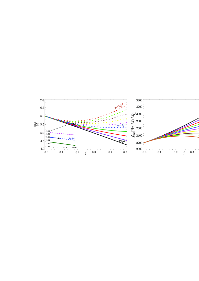
Figure 3: Left: the radial position of the marginally stable circular orbit $r_{\mathrm{ms}}$; dashed lines correspond to the inferred location of the marginally stable orbit being below the surface of the neutron star. Right: the orbital frequency $f_{\mathrm{ms}}$ at $r_{\mathrm{ms}}$.

In general relativity, stable circular orbital motion is restricted to radii larger than that of the marginally stable orbit which, in the external Hartle–Thorne geometry, is given by

$$r_{\mathrm{ms}}=6M\left[1\mp j\frac{2}{3}\sqrt{\frac{2}{3}}+j^{2}\left(\frac{251647}{2592}-240\ln\frac{3}{2}\right)+q\left(-\frac{9325}{96}+240\ln\frac{3}{2}\right)\right],$$ (8)

with the $-$ and $+$ referring to co-rotating and counter-rotating motion respectively. Only outside this orbit can quasi-circular geodesic motion be stable, giving rise to possibly observable quasi-periodic oscillatory effects. Properties of the marginally stable orbit have been discussed in detail in, for example, Török et al. (2014); Cipolletta et al. (2017) and are shown here in Fig. 3. In the left frame, one can see that the radius of the marginally stable orbit $r_{ms}$ always decreases with increasing $j$ near to $j=0$, but can reach a minimum and then become increasing for higher values of $j$ if $q/j^{2}$ is large enough. This sort of behavior can have a relevant impact on the observed distribution of rotational frequencies of QPO sources (Török et al., 2014). The position of the surface of the neutron star can be calculated from the universal relations (Yagi & Yunes, 2006) (given that $q/j^{2}$ is directly related to the inverse compactness of the star $R/M$); results can be seen on the left side of Fig. 3. In the zoomed area, note the curve for $q/j^{2}=5$ where a dot indicates the position of the surface. For the rest of the specified values of $q/j^{2}$, $r_{\mathrm{ms}}$ is situated above the surface for $q/j^{2}<5$ and below the surface for $q/j^{2}>5$, within the range of $j$ shown.

The formula for the orbital frequency at $r_{\mathrm{ms}}$ can be calculated up to second order in the star’s angular velocity as

$$f_{\mathrm{ms}}=\frac{c^{3}}{2\pi GM6\sqrt{6}}\left[1+\frac{11j}{6\sqrt{6}}+\frac{1}{864}j^{2}\left(-160583+397710\ln\frac{3}{2}\right)+\frac{5}{32}q\left(1193-2946\ln\frac{3}{2}\right)\right].$$ (9)

The right panel of Figure 3 shows $f_{\mathrm{ms}}$ plotted against $j$ as calculated from this.

In the discussion above, we have used the term “marginally stable orbit” thinking only of the external vacuum region but, in reality, for a given model of the neutron star, this location may not exist in the external region: the equatorial radius of the star $R_{\mathrm{eq}}$ with given parameters $M$, $j$ and $q$ can be larger than the $r_{\mathrm{ms}}$ as calculated in a vacuum exterior space-time with the same parameters. In the remainder of this paper, we will be using the term “innermost stable circular orbit” (ISCO) in a non standard way, to refer either to the orbit at $r_{\mathrm{ms}}$, if it exists outside the star, or otherwise to a surface-skimming orbit at $R_{\mathrm{eq}}$. One should bear in mind that, in practice, a particle on a surface-skimming orbit would be subject to various physical effects which we are not including here.

In order to obtain a complementary point of view, in Figure 4 we show the radial profiles of the orbital and epicyclic frequencies for specified values of $j$, together with the profiles for the local value of the Keplerian frequency $\nu_{\mathrm{K}}$. One can see that the influence of the parameters $j$ and $q/j^{2}$ increases with decreasing radius, and is relatively small at radii $r\sim 10M$ for all of the three frequency profiles; in all three cases, the influence of $q/j^{2}$ increases with increasing $j$. For the orbital frequency, the role of the parameters $j$ and $q$ is the smallest, and it is significantly stronger for the profile of the vertical epicyclic frequency which has a similar behavior to that of the orbital frequency. The most important influence is in the case of the radial epicyclic frequency – the shift of the marginally stable circular orbit, corresponding to the radius where the radial epicyclic frequency vanishes, is significantly shifted even for spin $j=0.1$. For $j=0.3$ it is shifted from $r_{\mathrm{ms}}\sim 5M$ for $q/j^{2}=1$ to $r_{\mathrm{ms}}\sim 5.8M$ for $q/j^{2}=10$, and in the extreme case of $j=0.5$, the shift is from $r_{\mathrm{ms}}\sim 4.4M$ for $q/j^{2}=1$ to $r_{\mathrm{ms}}\sim 6.6M$ for $q/j^{2}=10$. Clearly, the role of the quadrupole moment is most significant for the radial epicyclic motion where it affects also the values at the maxima of radial epicyclic frequency.

One can see that, contrary to the case of the Kerr black hole spacetime, the vertical epicyclic frequency can be larger than the orbital frequency. This phenomenon has been observed also for Newtonian quadrupole gravitational fields (Gondek-Rosińska et al., 2014) and general relativistic solutions with multipole structure of the Manko type (Pappas, 2012). A similar crossing of the radial profiles of the radial and vertical oscillations has been found also for axisymmetric string loops in the Kerr black hole spacetime (Stuchlík & Kološ, 2014, 2015). This type of behavior was discovered by Morsink & Stella (1999) around rapidly rotating neutron stars with a very stiff equation of state and was also found for analytical approximations to these spacetimes (Pappas, 2012; Pappas & Apostolatos, 2013). Recently it has been discussed by Kluźniak & Rosińska (2013) in the context of Newtonian gravity and then further considered by Gondek-Rosińska et al. (2014) for rapidly rotating relativistic strange stars. Its relation to the higher order multipole moments of spacetimes around compact objects can be found in Pappas (2017)).

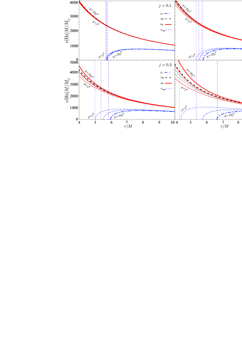
Figure 4: The radial profile of the orbital frequency $\nu_{\mathrm{K}}$ and the epicyclic frequencies $\nu_{\mathrm{r}}$, $\nu_{\mathrm{\theta}}$ for $j=0.1,0.2,0.3,0.5$. The increasing thickness of the lines represents increasing values of $q/j^{2}=1,~{}5,~{}10$. The vertical dotted lines are calculated values of $r_{\mathrm{ms}}$ for each $q/j^{2}$, as given by equation (8). Note that stable circular orbits are possible only for $r>r_{\mathrm{ms}}$.

Clearly, the quadrupole parameter $q/j^{2}$ is playing an important role and this needs to be investigated further. In the next subsections we will look in more detail at the value of the radial epicyclic frequency at its maximum.

3.2 Local extrema of the radial epicyclic frequency

Of the three frequencies describing orbital motion investigated above, the radial epicyclic frequency is the only one that is non-monotonic in $r/M$ for small $j$. We will now investigate further the radius at which $\nu_{\mathrm{r}}$ has its maximum and the values which it takes there. The location of the maximum can be found by solving the equation

$$\frac{d\nu_{r}}{dr}=0.$$ (10)

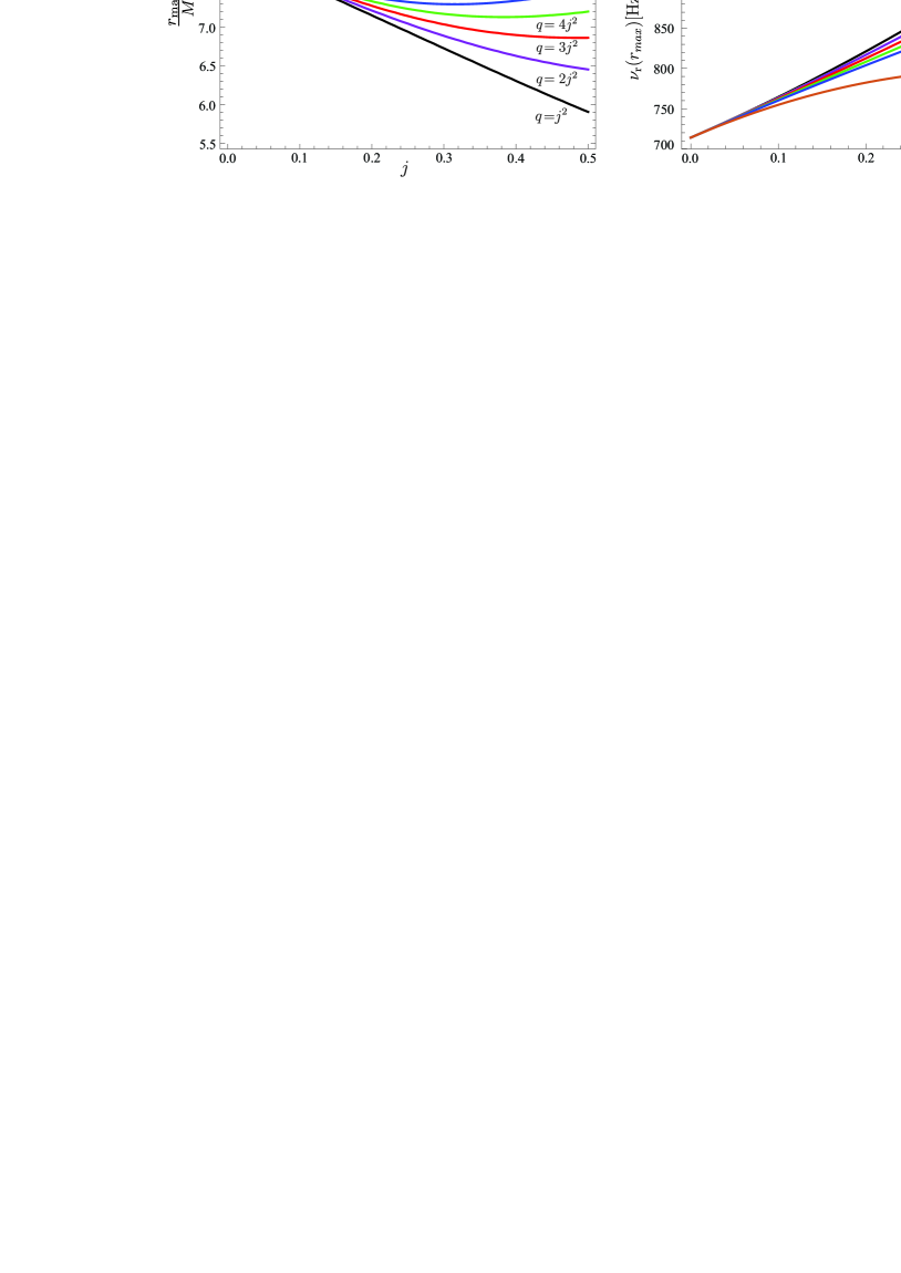
Figure 5: Left: the radius at which the profile of the radial epicyclic frequency $\nu_{\mathrm{r}}$ has its maximum. Right: the value of $\nu_{\mathrm{r}}$ at $r_{\mathrm{max}}$.

The solution can be found analytically, and is

$$r_{\mathrm{max}}=8M\left[1-\frac{47}{64\sqrt{2}}j+\frac{-12596207+43683840\ln\frac{4}{3}}{147456}j^{2}-\frac{5}{576}\left(-9835+34128\ln\frac{4}{3}\right)q\right]$$ (11)

The radial epicyclic frequency at $r_{\mathrm{max}}$ is then given by

$$\nu_{\mathrm{r}}(r_{\mathrm{max}})=\sqrt{\frac{c^{3}}{64\sqrt{2}\pi GM}\left[1+\frac{15}{16\sqrt{2}}j+\frac{-3972109+13824000\ln\frac{4}{3}}{8192}j^{2}+\frac{5}{16}q\left(1553-5400\ln\frac{4}{3}\right)\right]},$$ (12)

or, in a simplified form,

$$\nu_{\mathrm{r}}(r_{\mathrm{max}})=\sqrt{\frac{714.011}{M}(1+0.663j+0.587j^{2}-0.15q)}.$$ (13)

The left panel of Figure 5 shows the locations of the maximum $r_{\mathrm{max}}$ plotted as a function of $j$, and the right panel shows the values of $\nu_{\mathrm{r}}$ at $r_{\mathrm{max}}$. One can see that $q/j^{2}$ is having an impact rather similar to that in the case of the marginally stable circular orbit, with a minimum appearing in the curves for larger values of $q/j^{2}$ and moving to smaller values of $j$ as $q/j^{2}$ is increased. From the right panel, one sees that the largest values of $q/j^{2}$ may even cause $\nu_{\mathrm{r}}(r_{\mathrm{max}})$ to become a decreasing function of $j$ at high enough rotation speeds.

3.3 Precession frequencies

For matter orbiting around neutron stars, the quantities that may be directly observable could be related to combinations of the epicyclic frequencies, rather than to the frequencies themselves. In particular, the precession frequencies (periastron or nodal) may play an important role.

The periastron precession frequency is given by

$$\nu_{\mathrm{P}}^{\mathrm{r}}=\nu_{K}-\nu_{r},$$ (14)

while the nodal precession frequency is given by

$$\nu_{\mathrm{P}}^{\mathrm{\theta}}=\nu_{K}-\nu_{\theta},$$ (15)

with $\nu_{K}$, $\nu_{r}$ and $\nu_{\theta}$ being given by equations (5), (6) and (7).

For calculation of precession frequencies, we again chose $j=0.1,0.2,0.3,0.5$ and we varied the quadrupole parameter $q$ in the range $q/j^{2}=1,2,3,4,5,10$ for each value of $j$. Results are plotted in Figures 6 and 7. In both cases, the impact of $q/j^{2}$ becomes progressively more significant as $j$ increases. Note that the nodal precession frequency can become negative, since the radial epicyclic frequency can be higher than the orbital frequency. For low values of $j$, this happens only if $q/j^{2}$ is large and then only very near to $r=3M$, while for larger values of $j$ it happens also for smaller $q/j^{2}$.

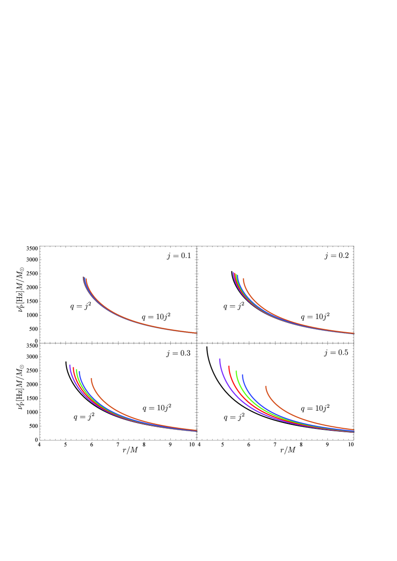
Figure 6: The radial profile of the periastron precession frequency $\nu_{\mathrm{P}}^{\mathrm{r}}$.

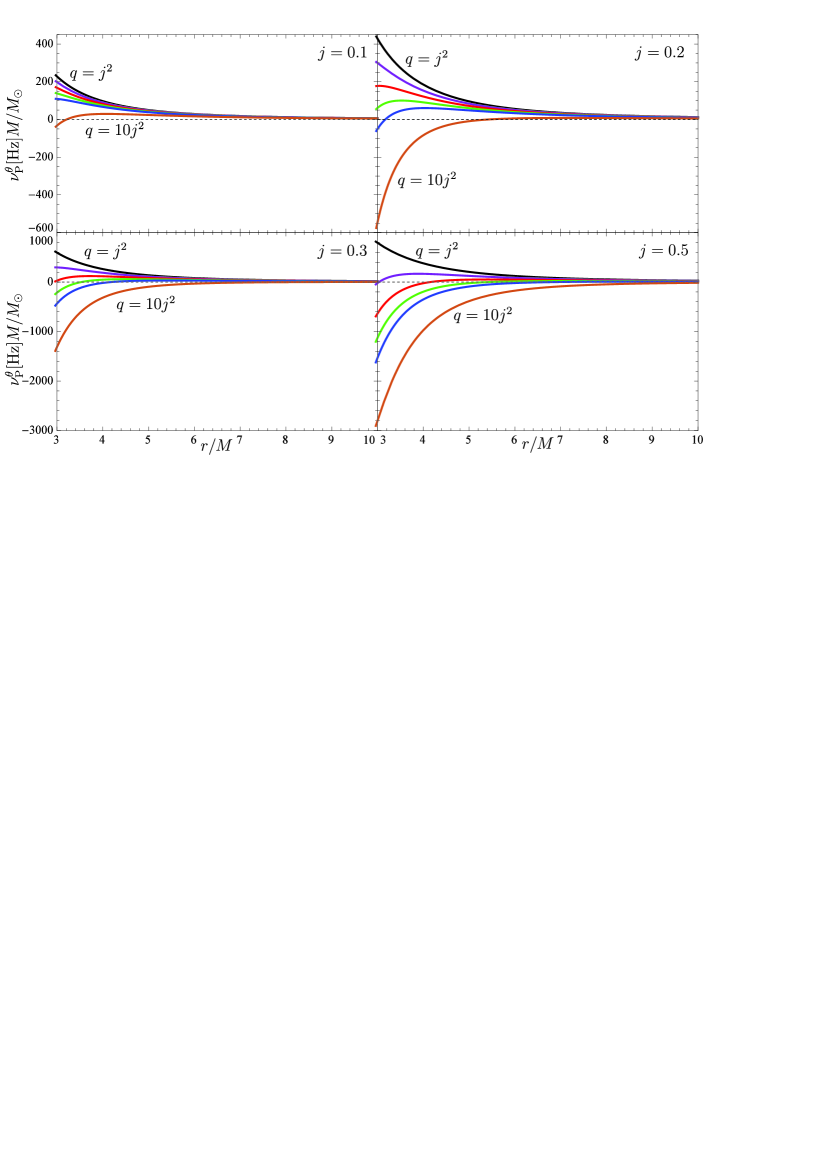
Figure 7: The radial profile of the nodal precession frequency $\nu_{\mathrm{P}}^{\mathrm{\theta}}$.

3.4 Comparison of the Keplerian frequency and the vertical epicyclic frequency

As mentioned previously, within Newtonian theory it has been found by Gondek-Rosińska et al. (2014) that the vertical epicyclic frequency can be larger than the frequency of orbital motion if the central object is sufficiently oblate and we have seen that this can happen also for neutron stars (in general relativity) even if they are not very non-spherical. Here, we calculate the ratio of vertical epicyclic frequency to Keplerian frequency of orbital motion, and investigate when it is larger than one. The square of the ratio of these two frequencies can be written as

$$\left[\frac{\nu_{\theta}(r;M,j,q)}{\nu_{K}(r;M,j,q)}\right]^{2}=1-jK(r)+j^{2}L(r)-qM(r),$$ (16)

where

$$K(r) = 4M^{3/2}r^{-3/2},$$

$$L(r) = \frac{3}{8}M^{-2}r^{-2}(8M^{4}+35M^{2}r^{2}-30Mr^{3}+15r^{4})+N(r),$$

$$M(r) = \frac{15}{8}M^{-2}(7M^{2}-6Mr+3r^{3})+N(r),$$

$$N(r) = \frac{45}{16}M^{-3}(M-r)(2M^{2}-2Mr+r^{2})\ln\left(\frac{r}{r-2M}\right).$$

We plot the results in Figure 8, marking the cases where the Keplerian frequency is equal to the vertical epicyclic frequency. These points correspond to situations where the relativistic nodal frequency vanishes and changes sign.

The position where the nodal frequency vanishes needs to be compared with that of the marginally stable circular geodesic for the values of $j$ and $q/j^{2}$ being used, because the effect of nodal frequency switching is relevant only in the regions where the circular geodesic motion is stable against perturbations, i.e., outward of the marginally stable circular orbit at $r_{\mathrm{ms}}$. We have calculated the locations of $r_{\mathrm{ms}}$ using the relation (8), and these are shown as vertical lines in Figure 8 with the line-style corresponding to that for the $\nu_{\theta}/\nu_{\mathrm{K}}$ profile with same value of $q/j^{2}$. We can see some cases (especially for low values of $j$) where $\nu_{\theta}/\nu_{\mathrm{K}}=1$ occurs at a radius below $r_{\mathrm{ms}}$. On the other hand, for higher values of $j$ and $q/j^{2}$, $\nu_{\theta}>\nu_{\mathrm{K}}$ can occur also for orbits that are stable with respect to radial perturbations.

We now investigate the locations where

$$\left[\frac{\nu_{\theta}(r;M,j,q)}{\nu_{K}(r;M,j,q)}\right]^{2}=1.$$ (17)

Since $\nu_{\theta}$ is always equal to $\nu_{\mathrm{K}}$ in the non-rotating Schwarzschild case, one cannot find the location for the nodal switching point as an expansion around the Schwarzschild value. The values of $q/j^{2}$ satisfying (17) are given by

$$\frac{q}{j^{2}}=1+\frac{64M^{9/2}\sqrt{r}-48jM^{5}}{15jr^{2}\left[-2M\left(7M^{2}-6Mr+3r^{2}\right)-3(M-r)\left(2M^{2}-2Mr+r^{2}\right)\ln\left(\frac{r}{r-2M}\right)\right]},$$ (18)

and in Figure 9 we plot these against $r/M$ for $j=0.2,0.3,0.4,0.5$. The dotted lines show the value of $r_{\mathrm{ms}}$ for each $j$ and the purple dashed line indicates the stellar surface; we have marked the point on each of the $j$ curves beyond which $r$ is greater than both of those limits.

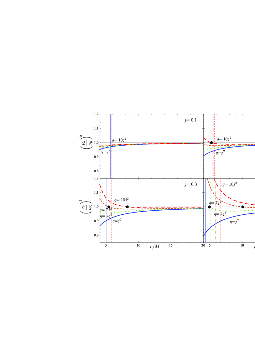
Figure 8: Points where the Keplerian and vertical epicyclic frequencies are equal.

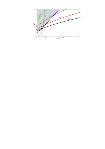
Figure 9: The value of $q/j^{2}$ giving $\nu_{\theta}=\nu_{\mathrm{K}}$ is plotted as a function of $r/M$ for various values of $j$. The dotted lines show the value of $r_{\mathrm{ms}}$ for each $j$ and the purple dashed line marks the stellar surface.

4 Models of twin HF QPOs and the frequency ratios in the Hartle–Thorne geometry

In the previous section we have investigated the behavior of the orbital, epicyclic and precession frequencies. We have seen that as $j$ increases, the role of the quadrupole term becomes increasingly important. In this section, we focus on particular combinations of frequencies that play key roles for models of QPOs - the twin peaks observed in power spectra of LMXBs. The origin of these peaks is still under investigation, but several candidate models are using frequencies associated with orbital motion around the central objects.

4.1 Frequency ratios of oscillatory modes for the twin HF QPO models

In this section we study the behavior of the frequencies of oscillatory modes given by some current models for the twin HF QPOs observed in atoll and Z-sources, where a neutron star is accreting matter from a low-mass companion (for the differences between atoll and Z-sources see Hasinger & van der Klis (1989)). We consider the specific models presented in Table 1, where we also give the combinations of frequencies that are attributed to the upper and lower observed peaks in each case. Our selection of models is based on Török et al. (2011). None of the models is currently uniquely preferred, because each of them has (different) theoretical problems. The RP (Relativistic Precession) model (Stella & Vietri, 1999) considers relativistic epicyclic motion of blobs at various radii in the inner parts of the accretion disc; The TD (Tidal Disruption) model (Čadež et al., 2008) proposes that the QPOs are generated by a tidal disruption of large accreting inhomogeneities; The WD (Warped Disk) model (Kato, 2001) considers a somewhat exotic disc geometry that causes a doubling of the observed lower QPO frequency; The ER (Epicyclic Resonance) model (Abramowicz & Kluźniak, 2001) involves different combinations of axisymmetric disk-oscillation modes; RP1 (Bursa, 2005) and RP2 (Török et al., 2007) use different combinations of non-axisymmetric disk-oscillation modes. We are considering here only geodesic oscillation models where the oscillatory modes are combinations of the orbital and epicyclic frequencies of near-circular geodesic motion in the equatorial plane.

Table 1: An overview of the orbital models of QPOs, with specification of the upper $\nu_{\mathrm{U}}$ and lower $\nu_{\mathrm{L}}$ frequencies.

Frequency	RP	TD	WD	RP1	RP2	ER
$\nu_{\mathrm{U}}$	$\nu_{\mathrm{K}}$	$\nu_{\mathrm{K}}+\nu_{\mathrm{rad}}$	$2\nu_{\mathrm{K}}-\nu_{\mathrm{rad}}$	$\nu_{\theta}$	$2\nu_{\mathrm{K}}-\nu_{\theta}$	$\nu_{\theta}$
$\nu_{\mathrm{L}}$	$\nu_{\mathrm{K}}-\nu_{\mathrm{rad}}$	$\nu_{\mathrm{K}}$	$2(\nu_{\mathrm{K}}-\nu_{\mathrm{rad}})$	$\nu_{\mathrm{K}}-\nu_{\mathrm{rad}}$	$\nu_{\mathrm{K}}-\nu_{\mathrm{rad}}$	$\nu_{\mathrm{rad}}$

In Figure 10 we show the radial profiles of the frequency ratio $\nu_{\mathrm{U}}/\nu_{\mathrm{L}}$ for all of the six QPO models being considered here.

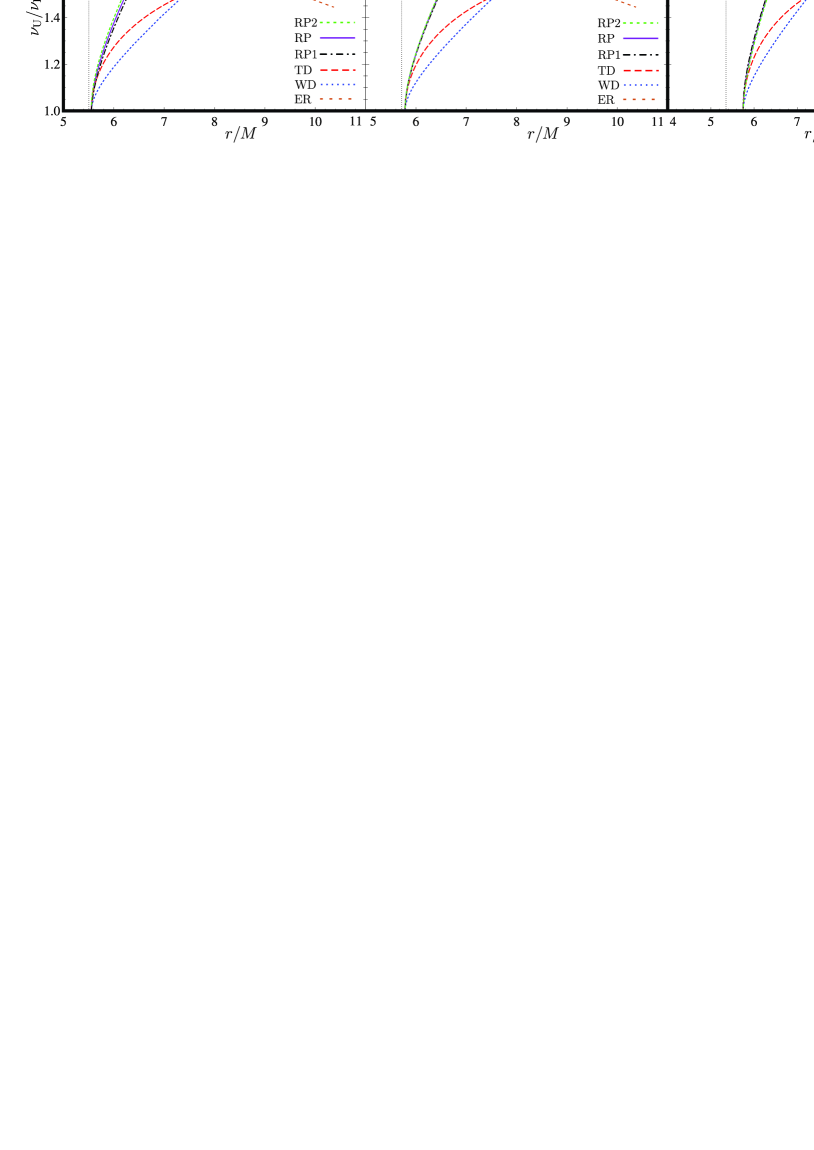
Figure 10: The orbital models of QPOs (with $j=0.1,~{}0.2,~{}0,3,~{}0.5$). The dependence of $\nu_{\mathrm{U}}/\nu_{\mathrm{L}}$ on $r/M$ is shown. The vertical dotted line indicates the location of the marginally stable orbit $r_{\mathrm{ms}}$, as given by equation (8), and the horizontal line indicates the ratio $\nu_{\mathrm{U}}~{}:~{}\nu_{\mathrm{L}}~{}=~{}3~{}:~{}2$.

As in the previous section, we use the values $j=0.1,0.2,0.3,0.5$, which includes the maximal range of the spin parameter $j$ for the Hartle–Thorne approximation (Urbanec et al., 2013), and for the quadrupole parameter $q$ we use values obtained from taking $q/j^{2}=1,3,5,10$, covering the most astrophysically relevant models for rotating neutron stars. It can be seen that for the RP models, the ratio $\nu_{\mathrm{U}}/\nu_{\mathrm{L}}=3/2$ occurs just slightly outside the location of the marginally stable orbit, meaning that the QPOs will generally be related to the region very close to the inner edge of the accretion disk, but for the TD and WD models the radius is larger and it is even more so for the ER model. However all of the considered models are giving the radius where $\nu_{\mathrm{U}}/\nu_{\mathrm{L}}=3/2$ as being between $r_{\mathrm{ms}}$ and $r=11M$.

We also note that the RP, RP1 and RP2 models give extremely similar profiles, with only very minor differences. The profiles of the WD and TD models are different, but they always cross each other at the frequency ratio $3:2$. For the ER model, the ratio diverges at the marginally stable orbit, since the radial epicyclic frequency has to vanish there, and this is the only case where the ratio decreases with increasing radius. In all of the models, the radial profiles depend only slightly on the quadrupole parameter for small values of $j<0.2$, but the dependence increases with increasing $j$, and for $0.3<j<0.5$ it can be very strong, especially close to the marginally stable orbit.

In Figure 11, we show these results plotted for each of the QPO models separately, using $j=0.1,0.2,0.3,0.5$, as before, and $q/j^{2}=1,2,3,4,5,10$. Here one can appreciate better the role of $j$ and $q/j^{2}$ for varying the position of marginally stable orbit. Note the qualitative difference between the results for the ER model and the others.

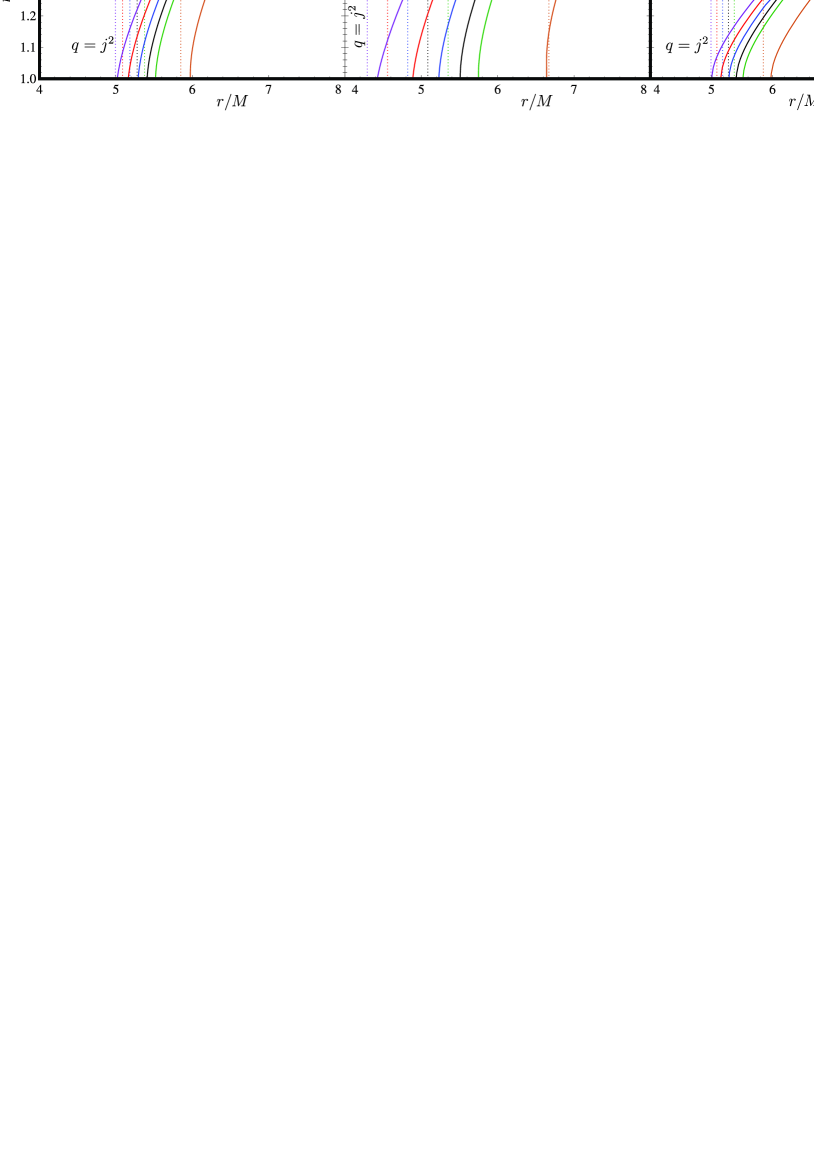
Figure 11: Individual results for each of the orbital QPO models: RP, RP1, RP2, TD, WD, ER (top left to bottom right). The ratio $\nu_{\mathrm{U}}/\nu_{\mathrm{L}}$ is plotted against $r/M$ for each model. The vertical dotted lines indicate the location of the marginally stable orbit $r_{\mathrm{ms}}$ for each value of $q$.

4.2 The frequency ratio $3:2$ in the twin HF QPO models

Observational data for QPOs demonstrates the importance of the frequency ratio $3:2$ (Boutelier et al., 2010) and so we have calculated how the location where this ratio is generated varies as a function of $j$. The left panels of Figure 12, show this for each of our QPO models for $q/j^{2}=1,2,3,4,5,10$. Note that the behavior of $r_{3:2}/M$ demonstrates a qualitatively similar behavior to that for the location of the marginally stable orbit: for small values of $q/j^{2}$, the resonance radius decreases with increasing spin, as for Kerr black holes, but for large enough $q/j^{2}$ it reaches a minimum and then increases again.

The right panels of Figure 12 show equivalent results for the ratio 5:4, which are quite similar.

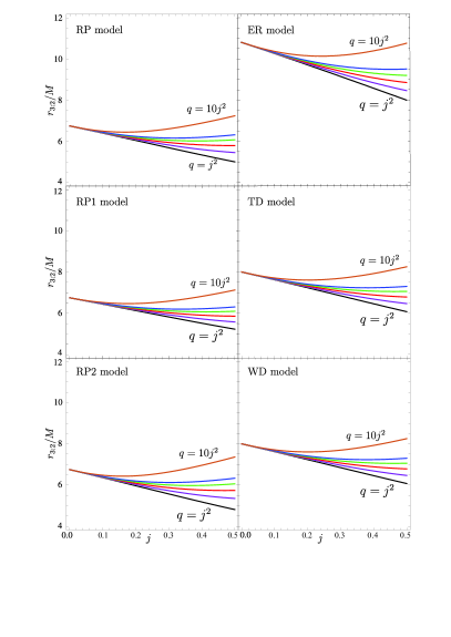
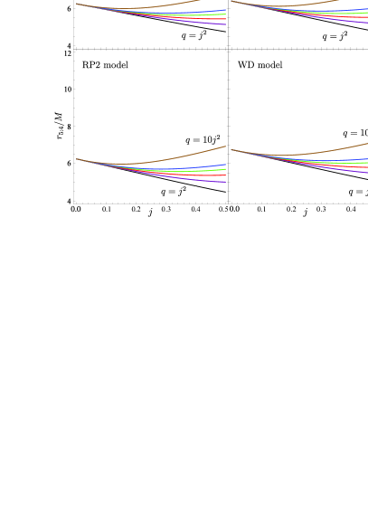
Figure 12: The locations where the resonant QPO ratios 3:2 and 5:4 are generated: For each of the models, $r_{3:2}/M$ (left panels) and $r_{5:4}/M$ (right panels) are plotted against $j$ for $q/j^{2}=1,2,3,4,5,10$.

5 Comparison of results from the Hartle–Thorne approach and the Lorene/nrotstar numerical code

In this section we test the range of validity of the Hartle–Thorne approach by comparing results obtained with it against ones given by the publicly available Lorene/nrotstar code (Gourgoulhon et al., 2016). We compare models having the same gravitational mass for a static non-rotating star $M_{0}$ and then keep constant the value of the central pressure (and the energy or enthalpy density) when we move to rotating models. We use the APR equation of state (Akmal et al., 1998) for making the comparison.

We focus on the quantity $\Delta f_{\mathrm{ISCO}}=f_{\mathrm{ISCO}}-f_{\mathrm{ISCO}}(f=0Hz)$, where $f_{\mathrm{ISCO}}$ is here the frequency at the innermost stable orbit (either the marginally stable circular orbit at $r=r_{\mathrm{ms}}$ or the equatorial surface-skimming orbit at $r=R_{\mathrm{eq}}$ when $R_{\mathrm{eq}}>r_{\mathrm{ms}}$, as discussed previously (see also Pappas (2015) for discussion of when the surface of the neutron star lies above/below $r_{\mathrm{ms}}$).

This quantity is zero in the non-rotating case and its leading order in the slow-rotation expansion goes as $f_{\mathrm{rot}}$ while the order of its first neglected term goes as $\mathcal{O}(f^{3}_{\mathrm{rot}})$, i.e. the relative error is of order $\mathcal{O}(f^{2}_{\mathrm{rot}})$. This is also the case for $\nu^{\theta}_{\mathrm{P}}$, but the quantities $f_{\mathrm{ISCO}}$ and $\nu_{P}^{r}$ have non-zero values for the non-rotating case, i.e. the leading term is of $\mathcal{O}(f^{0}_{\mathrm{rot}})$, and since the first neglected term is again $\mathcal{O}(f^{3}_{\mathrm{rot}})$, this means that the relative error is of order $\mathcal{O}(f^{3}_{\mathrm{rot}})$, one order higher than that for $\nu^{\theta}_{\mathrm{P}}$. Because of this $\nu^{\theta}_{\mathrm{P}}$ is likely to be the quantity most liable to error and so it is sensible to use as our key test quantity $\Delta f_{\mathrm{ISCO}}=f_{\mathrm{ISCO}}-f_{\mathrm{ISCO}}(f=0Hz)$ which has an error of the same order as the most sensitive quantity of interest. This is not a foolproof argument because of different coefficients in the expansions of the quantities concerned, but it should be a reasonable guide.

For the ISCO frequency in the Hartle–Thorne approach, we calculate a gravitational mass $M$ for the rotating star, a dimensionless angular momentum $J/M_{0}^{2}$ and a dimensionless quadrupole moment $Q/M_{0}^{3}$, use these to calculate the radius $r_{\mathrm{ms}}$ from eq. (8) and then find the Keplerian frequency at this radius using eq. (5). If $r_{\mathrm{ms}}$ is less than $R_{\mathrm{eq}}$, then the latter is used instead in eq. (5). For the gravitational mass of the non-rotating star we take $M_{0}=1.2,~{}1.4,~{}1.6,~{}1.8M_{\odot}$. The rotational frequencies are taken up to the frequency where the difference between the Hartle–Thorne and Lorene values for $\Delta f_{\mathrm{ISCO}}$ reaches $\sim 10\%$. The results of the comparison are shown in Figures 13 and 14, where we show also the 5% and 10% intervals around the Lorene values. The positive gradients correspond to $r_{\mathrm{ms}}$ being used, and the negative gradients to $R_{\mathrm{eq}}$. Since we are here dealing with specific models, the location of the stellar surface is directly known.

The two approaches are in excellent agreement for the lower rotation frequencies, as expected; when differences begin to emerge, Hartle–Thorne is giving higher values for $\Delta f_{\mathrm{ISCO}}$ in all cases. We see that for lower masses the difference between the Lorene and Hartle–Thorne values of $\Delta f_{\mathrm{ISCO}}$ are smaller than 10% up to frequencies of about 500Hz, while for higher masses the rotational frequencies can go up to 700Hz (for $M=1.6M_{\odot}$) or 1000Hz (for $M=1.8M_{\odot}$). Since it is generally believed that neutron stars in QPO sources have accreted matter from the companion star they should have rather high masses.

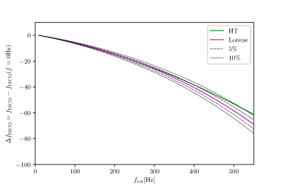
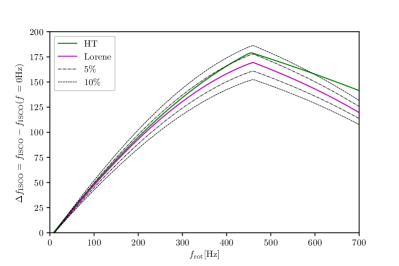
Figure 13: $\Delta f_{\mathrm{ISCO}}$ is plotted as a function of $f_{\mathrm{rot}}$ as calculated using the Hartle–Thorne and Lorene approaches. The gravitational mass of the non-rotating star is $M=1.2M_{\odot}$ (left) and $M=1.4M_{\odot}$ (right). See text for details.

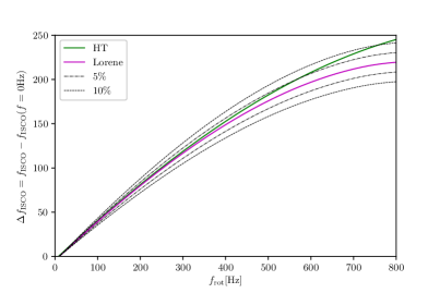
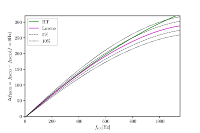
Figure 14: $\Delta f_{\mathrm{ISCO}}$ is plotted as a function of $f_{\mathrm{rot}}$ as calculated using the Hartle–Thorne and Lorene approaches. The gravitational mass of the non-rotating star is $M=1.6M_{\odot}$ (left) and $M=1.8M_{\odot}$ (right). See text for details.

6 Summary

We have examined the behavior of the orbital frequency, the radial epicyclic frequency and the vertical epicyclic frequency in the external Hartle–Thorne geometry for rotating compact stars. The primary parameters of the geometry are the gravitational mass $M$, the angular momentum $J$ and the quadrupole moment $Q$ and we have calculated the corresponding values for these from models of neutron stars constructed using realistic equations of state for nuclear matter. Our approach can be applied for any future equation of state if the universal relations are used as described in Section 2. Apart from the individual frequencies, we have also investigated the behavior of combinations of them which are involved in some models for QPOs observed in X-rays from LMXBs.

We have seen that the dimensionless angular momentum $j$ and dimensionless quadrupole moment $q$ play an important role for the behavior of the orbital and epicyclic frequencies, especially for the ratio between the vertical epicyclic frequency and the Keplerian frequency, becoming particularly important for stars rotating with the higher angular velocities. Our investigation was motivated by the observations of QPOs in the X-ray spectra of LMXBs and we have investigated the behavior of the frequencies relevant for several of the models proposed for explaining these.

It may seem redundant to spend time with more models, but at present we do not know which model may be relevant for the sources of QPOs and are not even sure whether only one model will be applicable for all of them. If the radiation does come from the accretion disc and is modulated by its oscillations, different oscillation modes may well be involved for different sources, depending on the geometry of the binary system. For example, if the equatorial plane of the compact object is the same as the orbital plane of the binary system, one may expect radial perturbations of the disc caused by matter falling in from the donor star. On the other hand, if the equatorial plane of the compact star is almost perpendicular to the orbital plane of the binary, one may expect vertical perturbations of the disk instead. This is something which may well clarify in the near future.

Finally we note that the results presented here can be relevant not only for the particular models mentioned in Section 4 but also for a wider class of orbital models. For instance, the maximum of the radial epicyclic frequency determines propagation of some discoseismic modes (Kato et al., 1998; Wagoner et al., 2001) and so there would be an application for making estimates of stellar spin rates based on association of QPOs with oscillations trapped near to the inner edge of thin accretion discs (Kato, 1989, 2001). This is illustrated in Figure 15 where we show the dependence of the maximum value of the radial epicyclic frequency $\nu_{\mathrm{r}}(r_{\mathrm{max}})$ for compact and highly oblate stars. Similar examples can be found for the vertical epicyclic frequency and models dealing with the Lense-Thirring precession effect (Ingram et al., 2009; Rosińska et al., 2014; Wiśniewicz et al., 2015; Ingram et al., 2015; Tsang & Pappas, 2016). The formulas given in Section 3 for determining the epicyclic frequencies (and the ratio between the vertical epicyclic frequency and the Keplerian frequency) can therefore be used in various applications, especially within the context of the universal relations.

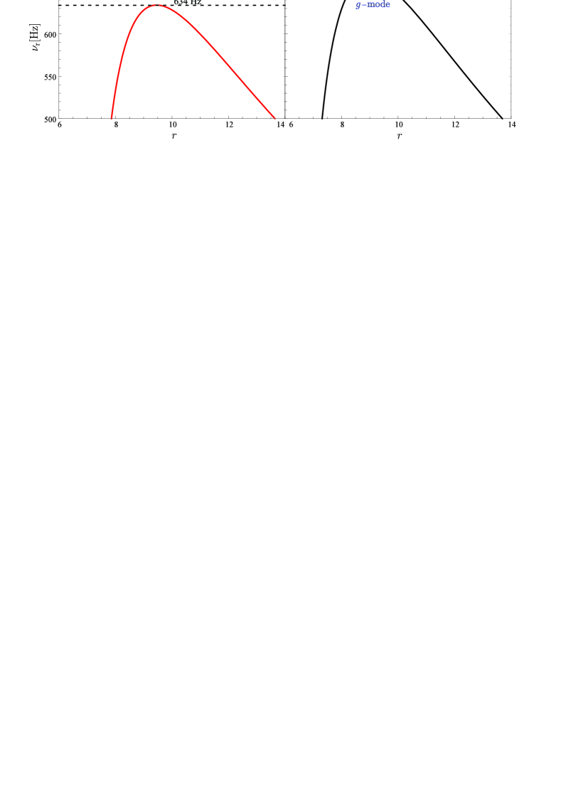
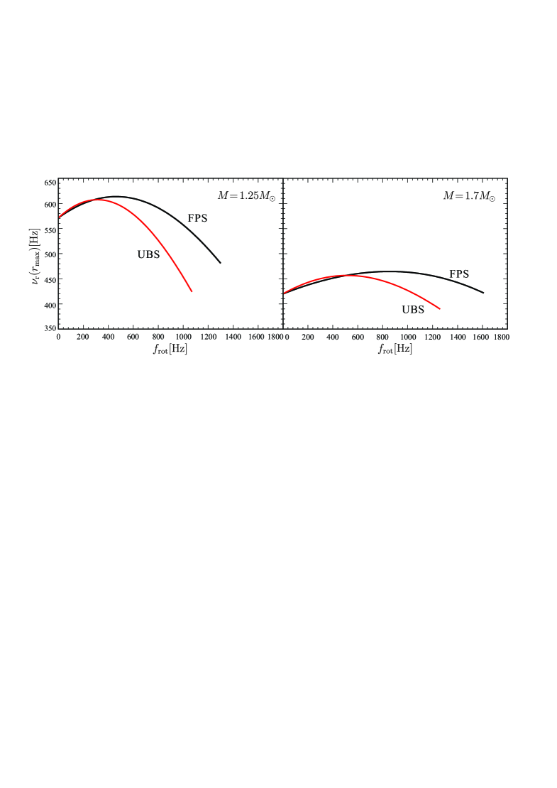
Figure 15: Upper: the radial profile of the radial epicyclic frequency $\nu_{\mathrm{r}}$ for stars with gravitational mass $1.2~{}M_{\odot}$ rotating with frequency of 580 Hz for two selected equations of state. The dashed horizontal lines indicate the values of $\nu_{\mathrm{r}}(r_{\mathrm{max}})$ determining the trapping of discoseismic g-modes. The dotted horizontal line indicates a particular value of the trapped g-mode frequency at 666 Hz which is allowed for the FPS EoS but not for UBS. Lower: the maximum radial epicyclic frequency, calculated using equation (12), plotted as a function of the stellar rotational frequency for stars with gravitational mass $1.25~{}M_{\odot}$ (left) and $1.7~{}M_{\odot}$ (right).

References

- Abramowicz et al. (2003a) Abramowicz, M. A., Almergren, G. J. E., Kluzniak, W., & Thampan, A. V. 2003a, gr qc, gr-qc/0312070
- Abramowicz et al. (2006) Abramowicz, M. A., Blaes, O. M., Horák, J., Kluźniak, W., & Rebusco, P. 2006, CQGra, 23, 1689
- Abramowicz et al. (2003b) Abramowicz, M. A., Bulik, T., Bursa, M., & Kluźniak, W. 2003b, A&A, 404, L21
- Abramowicz & Kluźniak (2001) Abramowicz, M. A., & Kluźniak, W. 2001, A&A, 374, L19
- Agrawal et al. (2005) Agrawal, B. K., Shlomo, S., & Au, V. K. 2005, Phys. Rev. C, 72, 014310
- Akmal et al. (1998) Akmal, A., Pandharipande, V. R., & Ravenhall, D. G. 1998, Phys. Rev. C, 58, 1804
- Antoniadis et al. (2013) Antoniadis, J., Freire, P. C. C., Wex, N., et al. 2013, Sci, 340, 448
- Bakala et al. (2012) Bakala, P., Urbanec, M., Šrámková, E., Stuchlík, Z., & Török, G. 2012, CQGra, 29, 065012
- Belloni et al. (2007) Belloni, T., Homan, J., Motta, S., Ratti, E., & Mendez, M. 2007, MNRAS, 379, 247
- Benhar et al. (2005) Benhar, O., Ferrari, V., Gualtieri, L., & Marassi, S. 2005, Phys. Rev. D, 72, 044028
- Berti & Stergioulas (2004) Berti, E., & Stergioulas, N. 2004, MNRAS, 350, 1416
- Berti et al. (2005) Berti, E., White, F., Maniopoulou, A., & Bruni, M. 2005, MNRAS, 358, 923
- Bonazzola & Gourgoulhon (1996) Bonazzola, S., & Gourgoulhon, E. 1996, A&A, 312, 675
- Bonazzola et al. (1998) Bonazzola, S., Gourgoulhon, E., & Marck, J.-A. 1998, Phys. Rev. D, 58, 104020
- Boshkayev et al. (2014) Boshkayev, K., Bini, D., Rueda, J., et al. 2014, GrCo, 20, 233
- Boshkayev et al. (2015) Boshkayev, K., Rueda, J., & Muccino, M. 2015, ARep, 59, 441
- Boutelier et al. (2010) Boutelier, M., Barret, D., Lin, Y., & Török, G. 2010, MNRAS, 401, 1290
- Bursa (2005) Bursa, M. 2005, in RAGtime 6/7: Workshops on black holes and neutron stars, ed. S. Hledík & Z. Stuchlík, 39–45
- Chakrabarti et al. (2014) Chakrabarti, S., Delsate, T., Gürlebeck, N., & Steinhoff, J. 2014, Phys. Rev. Lett., 112, 201102
- Chandrasekhar & Miller (1974) Chandrasekhar, S., & Miller, J. C. 1974, MNRAS, 167, 63
- Cipolletta et al. (2017) Cipolletta, F., Cherubini, C., Filippi, S., Rueda, J. A., & Ruffini, R. 2017, Phys. Rev. D, 96, 024046
- de Avellar et al. (2017) de Avellar, M. G., Porth, O., Younsi, Z., & Rezzolla, L. 2017, ArXiv e-prints, arXiv:1709.07706
- Demorest et al. (2010) Demorest, P. B., Pennucci, T., Ransom, S. M., Roberts, M. S. E., & Hessels, J. W. T. 2010, Nature, 467, 1081
- Doneva et al. (2015) Doneva, D. D., Yazadjiev, S. S., & Kokkotas, K. D. 2015, Phys. Rev. D, 92, 064015
- Doneva et al. (2014a) Doneva, D. D., Yazadjiev, S. S., Staykov, K. V., & Kokkotas, K. D. 2014a, Phys. Rev. D, 90, 104021
- Doneva et al. (2014b) Doneva, D. D., Yazadjiev, S. S., Stergioulas, N., & Kokkotas, K. D. 2014b, ApJ, 781, L6
- Fragile et al. (2016) Fragile, P. C., Straub, O., & Blaes, O. 2016, MNRAS, 461, 1356
- Friedman & Stergioulas (2013) Friedman, J. L., & Stergioulas, N. 2013, Rotating Relativistic Stars (Cambridge, UK: Cambridge University Press)
- Gandolfi et al. (2010) Gandolfi, S., Illarionov, A. Y., Fantoni, S., et al. 2010, MNRAS, 404, L35
- Gilfanov et al. (2003) Gilfanov, M., Revnivtsev, M., & Molkov, S. 2003, A&A, 410, 217
- Gondek-Rosińska et al. (2014) Gondek-Rosińska, D., Kluźniak, W., Stergioulas, N., & Wiśniewicz, M. 2014, Phys. Rev. D, 89, 104001
- Gourgoulhon et al. (2016) Gourgoulhon, E., Grandclément, P., Marck, J.-A., Novak, J., & Taniguchi, K. 2016, LORENE: Spectral methods differential equations solver, Astrophysics Source Code Library, , , ascl:1608.018
- Gutierrez-Ruiz et al. (2013) Gutierrez-Ruiz, A. F., Valenzuela-Toledo, C. A., & Pachon, L. A. 2013, Universitas Scientiarum, 19, arXiv:1309.6396
- Hartle (1967) Hartle, J. B. 1967, ApJ, 150, 1005
- Hartle & Thorne (1968) Hartle, J. B., & Thorne, K. S. 1968, ApJ, 153, 807
- Hasinger & van der Klis (1989) Hasinger, G., & van der Klis, M. 1989, A&A, 225, 79
- Haskell et al. (2014) Haskell, B., Ciolfi, R., Pannarale, F., & Rezzolla, L. 2014, MNRAS, 438, L71
- Hessels et al. (2006) Hessels, J. W. T., Ransom, S. M., Stairs, I. H., et al. 2006, Sci, 311, 1901
- Ingram & Done (2010) Ingram, A., & Done, C. 2010, MNRAS, 405, 2447
- Ingram et al. (2009) Ingram, A., Done, C., & Fragile, P. C. 2009, MNRAS, 397, L101
- Ingram et al. (2015) Ingram, A., Maccarone, T. J., Poutanen, J., & Krawczynski, H. 2015, ApJ, 807, 53
- Kato (1989) Kato, S. 1989, PASJ, 41, 745
- Kato (2001) —. 2001, PASJ, 53, 1
- Kato (2004) —. 2004, PASJ, 56, 905
- Kato et al. (1998) Kato, S., Fukue, J., & Mineshige, S., eds. 1998, Black-hole accretion disks
- Kluzniak & Abramowicz (2001) Kluzniak, W., & Abramowicz, M. A. 2001, AcPPB, 32, 3605
- Kluźniak & Rosińska (2013) Kluźniak, W., & Rosińska, D. 2013, MNRAS, 434, 2825
- Kostić et al. (2009) Kostić, U., Čadež, A., Calvani, M., & Gomboc, A. 2009, A&A, 496, 307
- Lo & Lin (2011) Lo, K.-W., & Lin, L.-M. 2011, ApJ, 728, 12
- Lorenz et al. (1993) Lorenz, C. P., Ravenhall, D. G., & Pethick, C. J. 1993, Phys. Rev. Lett., 70, 379
- Luk & Lin (2018) Luk, S.-S., & Lin, L.-M. 2018, ApJ, 861, 141
- Maselli et al. (2013) Maselli, A., Cardoso, V., Ferrari, V., Gualtieri, L., & Pani, P. 2013, Phys. Rev. D, 88, 023007
- Méndez (2006) Méndez, M. 2006, MNRAS, 371, 1925
- Miller (1977) Miller, J. C. 1977, MNRAS, 179, 483
- Mishra et al. (2017) Mishra, B., Vincent, F. H., Manousakis, A., et al. 2017, MNRAS, 467, 4036
- Montero & Zanotti (2012) Montero, P. J., & Zanotti, O. 2012, MNRAS, 419, 1507
- Morsink & Stella (1999) Morsink, S. M., & Stella, L. 1999, ApJ, 513, 827
- Nozawa et al. (1998) Nozawa, T., Stergioulas, N., Gourgoulhon, E., & Eriguchi, Y. 1998, A&AS, 132, 431
- Pachón et al. (2012) Pachón, L. A., Rueda, J. A., & Valenzuela-Toledo, C. A. 2012, ApJ, 756, 82
- Pani et al. (2015) Pani, P., Gualtieri, L., & Ferrari, V. 2015, Phys. Rev. D, 92, 124003
- Pappas (2012) Pappas, G. 2012, MNRAS, 422, 2581
- Pappas (2015) —. 2015, MNRAS, 454, 4066
- Pappas (2017) —. 2017, MNRAS, 466, 4381
- Pappas & Apostolatos (2012a) Pappas, G., & Apostolatos, T. A. 2012a, Phys. Rev. Lett., 108, 231104
- Pappas & Apostolatos (2012b) —. 2012b, ArXiv e-prints, arXiv:1211.6299
- Pappas & Apostolatos (2013) —. 2013, MNRAS, 429, 3007
- Pappas & Apostolatos (2014) —. 2014, Physical Review Letters, 112, 121101
- Parthasarathy et al. (2017) Parthasarathy, V., Kluzniak, W., & Cemeljic, M. 2017, ArXiv e-prints, arXiv:1703.05036
- Paschalidis & Stergioulas (2017) Paschalidis, V., & Stergioulas, N. 2017, LRR, 20, 7
- Reina (2016) Reina, B. 2016, MNRAS, 455, 4512
- Reina et al. (2017) Reina, B., Sanchis-Gual, N., Vera, R., & Font, J. A. 2017, MNRAS, 470, L54
- Reina & Vera (2015) Reina, B., & Vera, R. 2015, CQGra, 32, 155008
- Rezzolla et al. (2003) Rezzolla, L., Yoshida, S., & Zanotti, O. 2003, MNRAS, 344, 978
- Ribeiro et al. (2017) Ribeiro, E. M., Méndez, M., Zhang, G., & Sanna, A. 2017, MNRAS, 471, 1208
- Rosińska et al. (2014) Rosińska, D., Kluźniak, W., Stergioulas, N., & Wiśniewicz, M. 2014, Phys. Rev. D, 89, 104001
- Sanabria-Gómez et al. (2010) Sanabria-Gómez, J. D., Hernández-Pastora, J. L., & Dubeibe, F. L. 2010, Phys. Rev. D, 82, 124014
- Sham et al. (2015) Sham, Y.-H., Chan, T. K., Lin, L.-M., & Leung, P. T. 2015, ApJ, 798, 121
- Silva et al. (2016) Silva, H. O., Sotani, H., & Berti, E. 2016, MNRAS, 459, 4378
- Šrámková et al. (2007) Šrámková, E., Torkelsson, U., & Abramowicz, M. A. 2007, A&A, 467, 641
- Staykov et al. (2016) Staykov, K. V., Doneva, D. D., & Yazadjiev, S. S. 2016, Phys. Rev. D, 93, 084010
- Steiner et al. (2005) Steiner, A. W., Prakash, M., Lattimer, J. M., & Ellis, P. J. 2005, Phys. Rep., 411, 325
- Stella & Vietri (1998) Stella, L., & Vietri, M. 1998, ApJ, 492, L59
- Stella & Vietri (1999) —. 1999, Phys. Rev. Lett., 82, 17
- Stella & Vietri (2001) Stella, L., & Vietri, M. 2001, in Astronomical Society of the Pacific Conference Series, Vol. 234, X-ray Astronomy 2000, ed. R. Giacconi, S. Serio, & L. Stella, 213
- Stergioulas & Friedman (1995) Stergioulas, N., & Friedman, J. L. 1995, ApJ, 444, 306
- Stone et al. (2003) Stone, J. R., Miller, J. C., Koncewicz, R., Stevenson, P. D., & Strayer, M. R. 2003, Phys. Rev. C, 68, 034324
- Stuchlík & Kološ (2014) Stuchlík, Z., & Kološ, M. 2014, Phys. Rev. D, 89, 065007
- Stuchlík & Kološ (2015) —. 2015, GReGr, 47, 27
- Török et al. (2008b) Török, G., Abramowicz, M. A., Bakala, P., et al. 2008b, AcA, 58, 15
- Török et al. (2008c) —. 2008c, AcA, 58, 113
- Török et al. (2005) Török, G., Abramowicz, M. A., Kluźniak, W., & Stuchlík, Z. 2005, A&A, 436, 1
- Török et al. (2008a) Török, G., Bakala, P., Stuchlík, Z., & Cech, P. 2008a, AcA, 58, 1
- Török et al. (2010) Török, G., Bakala, P., Šrámková, E., Stuchlík, Z., & Urbanec, M. 2010, ApJ, 714, 748
- Török et al. (2012) Török, G., Bakala, P., Šrámková, E., et al. 2012, ApJ, 760, 138
- Török et al. (2016) Török, G., Goluchová, K., Horák, J., et al. 2016, MNRAS, 457, L19
- Török et al. (2017a) Török, G., Goluchová, K., Šrámková, E., et al. 2017a, ArXiv e-prints, arXiv:1710.10901
- Török et al. (2017b) Török, G., Goluchová, K., Šrámková, E., et al. 2017b, in Proceedings of RAGtime 17–19, 17–19/23–26 Oct., 1–5 Nov., 2015/2016/2017, Opava, Czech Republic, ed. S. Hledík & Z. Stuchlík, 523–531
- Török et al. (2011) Török, G., Kotrlová, A., Šrámková, E., & Stuchlík, Z. 2011, A&A, 531, A59+
- Török et al. (2007) Török, G., Stuchlík, Z., & Bakala, P. 2007, Central European Journal of Physics, 5, 457
- Török et al. (2014) Török, G., Urbanec, M., Adámek, K., & Urbancová, G. 2014, A&A, 564, L5
- Tsang & Pappas (2016) Tsang, D., & Pappas, G. 2016, ApJ, 818, L11
- Urbanec et al. (2010) Urbanec, M., Beták, E., & Stuchlík, Z. 2010, AcA, 60, 149
- Urbanec et al. (2013) Urbanec, M., Miller, J. C., & Stuchlík, Z. 2013, MNRAS, 433, 1903
- Čadež et al. (2008) Čadež, A., Calvani, M., & Kostić, U. 2008, A&A, 487, 527
- van der Klis (2006) van der Klis, M. 2006, Stellar X-Ray Sources (Cambridge: ed. W. H. G. Lewin, Cambridge University Press), 39–112
- Wagoner (1999) Wagoner, R. V. 1999, Phys. Rep., 311, 259
- Wagoner et al. (2001) Wagoner, R. V., Silbergleit, A. S., & Ortega-Rodríguez, M. 2001, ApJ, 559, L25
- Weber (1999) Weber, F., ed. 1999, Pulsars as astrophysical laboratories for nuclear and particle physics
- Weber & Glendenning (1992) Weber, F., & Glendenning, N. K. 1992, ApJ, 390, 541
- Wiśniewicz et al. (2015) Wiśniewicz, M., Gondek-Rosińska, D., Kluźniak, W., & Stergioulas, N. 2015, arXiv, arXiv:1503.06636
- Wolfram Research (2018) Wolfram Research, I. 2018, Mathematica, Version 11.3, , , Champaign, IL
- Yagi et al. (2014) Yagi, K., Kyutoku, K., Pappas, G., Yunes, N., & Apostolatos, T. A. 2014, Phys. Rev. D, 89, 124013
- Yagi & Yunes (2006) Yagi, K., & Yunes, N. 2006, ArXiv e-prints, gr-qc/1608.02582v1
- Yagi & Yunes (2013a) —. 2013a, Sci, 341, 365
- Yagi & Yunes (2013b) —. 2013b, Phys. Rev. D, 88, 023009