The far-infrared polarization spectrum of $\rho$ Ophiuchi A from HAWC+/SOFIA observations

Abstract

We report on polarimetric maps made with HAWC+/SOFIA toward $\rho$ Oph A, the densest portion of the $\rho$ Ophiuchi molecular complex. We employed HAWC+ bands C ($89\,\mu$m) and D ($154\,\mu$m). The slope of the polarization spectrum was investigated by defining the quantity $\mathcal{R}_{DC}=p_{D}/p_{C}$, where $p_{C}$ and $p_{D}$ represent polarization degrees in bands C and D, respectively. We find a clear correlation between $\mathcal{R}_{DC}$ and the molecular hydrogen column density across the cloud. A positive slope ($\mathcal{R}_{DC}$ $>$ 1) dominates the lower density and well illuminated portions of the cloud, that are heated by the high mass star Oph S1, whereas a transition to a negative slope ($\mathcal{R}_{DC}$ $<$ 1) is observed toward the denser and less evenly illuminated cloud core. We interpret the trends as due to a combination of: (1) Warm grains at the cloud outskirts, which are efficiently aligned by the abundant exposure to radiation from Oph S1, as proposed in the radiative torques theory; and (2) Cold grains deep in the cloud core, which are poorly aligned due to shielding from external radiation. To assess this interpretation, we developed a very simple toy model using a spherically symmetric cloud core based on Herschel data, and verified that the predicted variation of $\mathcal{R}_{DC}$ is consistent with the observations. This result introduces a new method that can be used to probe the grain alignment efficiency in molecular clouds, based on the analysis of trends in the far-infrared polarization spectrum.

1 Introduction

It is generally believed that the magnetic field that permeates the interstellar medium (ISM) play an important role in the formation of stars and planets (e.g., Mouschovias et al., 2006; McKee & Ostriker, 2007; Krumholz, 2014; Li et al., 2014). The field has a tendency to become “frozen into” the partially ionized interstellar gas. In regions where the magnetic field energy density is subdominant to the kinetic energy of the matter, gas dynamics will influence magnetic field morphology. This effect has been observed for Hi shells (Heiles, 1998; Fosalba et al., 2002; Santos et al., 2011; Frisch & Dwarkadas, 2017; Soler et al., 2018) as well as at the edges of Hii regions (Pavel & Clemens, 2012; Santos et al., 2012, 2014; Planck Collaboration Int. XXXIV, 2016). Another crucial effect is the force exerted by the field on the gas. This force may generate filamentary structure by guiding of turbulent gas flows (Nagai et al., 1998; Nakamura & Li, 2008; Li et al., 2015), and it may suppress the fragmentation of filaments, thereby partly explaining the low efficiency of the star formation process (Hosking & Whitworth, 2004; Myers et al., 2013). Observations of interstellar polarization are the most widely adopted technique to map the magnetic field in the ISM, but in order to use dust polarimetry to study magnetic fields, one needs to understand magnetic alignment of interstellar dust grains. In recent years it has become feasible to carry out detailed, large-scale observations of the plane-of-sky orientations of the magnetic field permeating the relatively denser, molecular phases of the ISM, by exploiting grain alignment. Dust alignment can be detected via polarimetry of starlight that has been transmitted through a medium of aligned grains (e.g., Hall, 1949; Hiltner, 1949; Serkowski et al., 1975; Heiles, 2000) or, more directly, by observing the polarized emission from the grains themselves (e.g., Hildebrand et al., 2000; Page et al., 2007; Planck Collaboration Int. XXXV, 2016; Fissel et al., 2016; Chuss et al., 2019).

The mechanism believed to be responsible for grain alignment is referred to as Radiative Torques, also known as B-RATs or simply RATs mechanism (for example, see Dolginov & Mitrofanov 1976; Draine & Weingartner 1996, 1997; Lazarian & Hoang 2007; Hoang & Lazarian 2008, and the reviews by Lazarian 2007 and Andersson et al. 2015). RATs theory posits individual non-spherical grains spinning about their short axes and having non-zero helicity. When surrounded by an anisotropic field of radiation having wavelength comparable to the grain size, such grains are expected to spin up, precess around the magnetic field, and gradually align with their shorter axes preferentially parallel to the magnetic field direction. From a purely observational perspective, the ease with which grains become aligned with the magnetic field is seen to be influenced by their size (Kim & Martin, 1995), possibly by their composition (Smith et al., 2000; Chiar et al., 2006; Lazarian & Hoang, 2018), and probably by their radiative environment, as discussed in detail below. Observational constraints such as these tend to be consistent with RATs theory but many open questions remain (e.g., Andersson & Potter, 2010; Andersson et al., 2011, 2015; Ashton et al., 2018).

For molecular sight-lines, we observe an anti-correlation between the polarization fraction of dust emission (or equivalently, the polarization fraction per unit optical depth for the case of polarization by selective extinction) and the column density (e.g., Arce et al., 1998; Whittet et al., 2008; Fissel et al., 2016; Santos et al., 2017). Possible explanations for this observed anti-correlation are: (1) a greater degree of field disorder within the observed beam along high-column density sight-lines; (2) a loss of polarizing efficiency for grains deep in molecular clouds; (3) a combination of both effects. The loss of polarization efficiency explanation could result from either changes in intrinsic grain properties for dense molecular regions (e.g., larger or rounder grains deep in clouds) or inefficient grain alignment for regions that are well-shielded from radiation. Indeed, RAT theory would predict that a loss of grain alignment should occur for locations that are so well shielded that not even near-infrared light from the interstellar radiation field can penetrate (Alves et al., 2014; Jones et al., 2015; Andersson et al., 2015). In addition, near-infrared spectro-polarimetry of the Taurus molecular cloud by Whittet et al. (2008) shows that along with loss of polarization fraction, the denser sight-lines exhibit a change in the wavelength dependence of the polarization that is consistent with a reduction in the fraction of grains that are aligned. They argue in favor of reduced grain alignment for well shielded regions as the main culprit for the anti-correlation, rather than field disorder or grain shape.

In this paper, we focus on a relatively unexplored observable, which is the polarization spectrum of the grains’ emission. In other words, we are concerned here with the fractional polarization as a function of wavelength. For the coldest regions of star forming molecular clouds, dust temperatures are in the range of $\sim 10-15\,$K, so the dust thermal radiation is mainly in the submillimeter and millimeter (peaking at $\approx 300\,\mu$m). However, dust temperatures can be much higher near newly formed early-type stars, and from these hotter dust grains we expect copious far-IR radiation at relatively shorter wavelengths ($\sim 50-200\,\mu$m). Using polarimetry from the Kuiper Airborne Observatory, Hildebrand et al. (1999) measured the first far-IR polarization spectra and found that the polarization fraction decreases with wavelength. After showing that the theoretically expected spectra for the simplest dust models were basically flat, they presented an idea for how to produce falling spectra: imagine that we have two kinds of regions along the same line of sight, namely some cold regions far from newly formed stars and hot regions closer to such sources. Further assume that the dust grains in the hot regions are much better aligned than the colder grains, perhaps due to RATs from these same sources. Since the hot regions with well aligned grains will be relatively brighter than the cold regions at the shorter wavelengths, we expect shorter wavelengths to be more polarized. Therefore, in this case it is clear that the polarization fraction will fall with increasing wavelength, i.e., we will find negatively sloped polarization spectra, as observed by Hildebrand et al. (1999).

During the two decades that have elapsed since the work by Hildebrand et al. (1999), much observational work has been done on far-infrared and submillimeter polarization spectra of star forming clouds, but the situation here is somewhat muddled. Ground-based observations have found positively sloped spectra in the submillimeter, suggesting a minimum in the polarization spectrum near $350\,\mu$m (Vaillancourt, 2002; Vaillancourt et al., 2008; Vaillancourt & Matthews, 2012; Zeng et al., 2013), but balloon-borne observations by the BLAST collaboration found flat submillimeter polarization spectra (Gandilo et al., 2016; Shariff et al., 2019). The difference may be due to the different column density regimes studied (Gandilo et al., 2016). There has also been progress on the theoretical side. Bethell et al. (2007) predicted that molecular clouds should have positive-slope polarization spectra in the far-IR ($\lambda<350\,\mu$m) and flat spectra in the submillimeter ($\lambda>350\,\mu$m). Draine & Fraisse (2009) modeled the diffuse ISM, finding a similar situation. Guillet et al. (2018) also modeled the diffuse ISM, finding that they could match the flat submillimeter-millimeter polarization spectra recently observed for the relatively tenuous regions by the Planck satellite (Planck Collaboration Int. XXII, 2015) and by BLAST (Ashton et al., 2018). From the theoretical perspective, the positive slopes in the far-IR are attributed to: (1) the fact that larger-sized grains ($\gtrapprox 0.2\,\mu$m) are relatively more efficiently aligned as compared to smaller-sized grains ($\lessapprox 0.2\,\mu$m) – this has been observationally verified by Kim & Martin (1995) and is also predicted from the RATs theory (e.g., Lazarian, 2007); and (2) the fact that different grain size populations follow different temperature distributions (even when subject to a uniform radiation field), with smaller grains being relatively warmer than larger grains due to their inefficiency in cooling radiatively (Li et al., 1999). As a result, the shorter wavelength emission within the far-infrared spectral range is dominated by warmer and relatively poorly aligned small grains (i.e., less polarized), while at long wavelengths, the emission from larger and better aligned grains is more significant (i.e., more polarized). In addition, composition can also play an important role (e.g., Draine & Fraisse, 2009).

The newly commissioned HAWC+ far-IR polarimeter for SOFIA (Dowell et al., 2010; Harper et al., 2018) allows us to revisit the topic of molecular cloud far-IR polarization spectra, but with better angular resolution and sensitivity. In this work, we present polarimetric observations of the nearby star forming region $\rho$ Oph A obtained with HAWC+ at two different far-IR wavelengths, $89\,\mu$m and $154\,\mu$m. The $\rho$ Oph A region is part of L1688, which in turn is part of the Ophiuchus molecular cloud. The distance to L1688 has been measured to be $137\pm 1\,$pc by Ortiz-León et al. (2017) via radio parallax measurements of 12 young stellar systems associated with this cloud. $\rho$ Oph A exhibits wide ranges of both temperature and column density (Motte et al., 1998), providing the opportunity to search for systematic variations in the polarization spectrum slope as a function of these parameters. The V-band extinction can reach levels larger than $100\,$mag (Friesen et al., 2017). Located at just $1.64\,$arcmin from the peak density (projected $0.065\,$pc), the high-mass star Oph S1 warms up the surrounding environment, causing a large temperature gradient (from approximately $20\,$K at the core to around $40\,$K near Oph S1). Oph S1 is the main heat source for $\rho$ Oph A, and is also associated with a $20\arcsec$ ultra-compact Hii region (Andre et al., 1988). The star is of type B3/4. It has almost reached the main sequence, and is now transitioning from a Herbig AeBe star into a magnetic B star (Andre et al., 1988; Hamaguchi et al., 2003). VLBA parallax observations show that Oph S1 lies at a distance of $138\pm 2\,$pc (Ortiz-León et al., 2017). Taking measurement errors into account, this is consistent with the distance measured by the same authors to L1688 as a whole (see above). $\rho$ Oph A contains numerous young stellar objects at different evolutionary stages (Classes 0, I, II, and III) as well as a population of starless cores (Motte et al., 1998; Pattle et al., 2015; Liseau et al., 2015).

In Section 2 below, we describe the data acquisition and reduction, and we detail the selection criteria used to identify data suitable for analysis. In Section 3 we describe this analysis, after first presenting our total intensity maps and polarization measurements. We discuss the results of our analysis in Section 4. Finally, Section 5 is a summary.

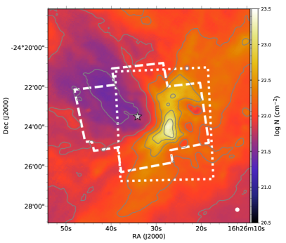
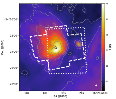
Figure 1: $\rho$ Oph A maps of the inferred molecular hydrogen (H₂) column density ($N$, left), and dust temperature ($T$, right), as derived from Herschel fluxes (see Section 3.2). The gray-colored star symbol indicates the position of Oph S1. The white dashed line and the white dotted line indicate the areas covered by HAWC+ bands C and D observations, respectively. In the left panel, the top contour represents $\log N(\mathrm{cm}^{-2})=23.1$, and the lower contours follow in subsequent steps of $\log N(\mathrm{cm}^{-2})=0.31$. In the right panel, the top contour represents a level of $T=37.5\,$K, with lower contours following in steps of $T=3.6\,$K. The circle at the bottom right of each panel represents the beam size (FWHM) of the Herschel data used to construct these maps.

2 Observations

Polarimetric data for $\rho$ Oph A were obtained using HAWC+/SOFIA (Harper et al., 2018) on May 5 2017 as part of the Guaranteed Time Observing (GTO) program. We used HAWC+ bands C ($89\,\mu$m) and D ($154\,\mu$m) that nominally provide angular resolutions of $7.8\arcsec$ and $13.6\arcsec$ FWHM (full width at half maximum), respectively. The standard matched-chop-nod method was used (Hildebrand et al., 2000) with a chopping frequency of $10.2$ Hz. For both bands, we used a chop angle of 154^∘ (measured from equatorial North and increasing to the East) and a chop throw of $480\arcsec$. These values were chosen in order to minimize the flux levels in our reference beams. A typical polarimetric observing block with HAWC+ consists of a set of 4 dithered observations, i.e., 4 independent pointings slightly displaced from each other forming a square pattern on the plane of the sky. Each such block is completed in approximately 15 minutes. The dithering displacement between individual observations was $24\arcsec$ for band C and $40\arcsec$ for band D.

The sky areas covered by the HAWC+ observations are indicated in Figure 1 using dashed lines (band C) and dotted lines (band D). This figure also shows, via color maps, the distributions of molecular hydrogen column density ($N$, left) and dust temperature ($T$, right) as derived from archival Herschel Space Observatory dust emission data (Pilbratt et al., 2010). Details of the methods we used to derive these maps are given in Section 3.2. For band C we obtained four observing blocks, with each observing block centered on a different sky position in order to increase total sky coverage. There was significant spatial overlap between the blocks. The sky area covered by our band C observations (dashed lines in Figure 1) is approximately centered on Oph S1, which roughly coincides with the location of peak dust temperature. For band D, two observing blocks were used, both with the same pointing. The band D map (dotted lines in Figure 1) is approximately centered on the cloud’s column density peak.

The polarimetry data presented here were processed using the HAWC+ data reduction pipeline version v1.3.0-beta3 (April 2018). As summarized by Harper et al. (2018), the pipeline consists of a series of sequential data processing steps,

which we briefly describe in the list below:

• Demodulation of the chopped data and removal of bad samples (due to tracking issues, half-wave-plate and nod movements, etc.);

• Flat-fielding of the demodulated data based on scans across extended sources, which were then transferred to our observations via flux measurements of an internal calibrator;

• Computation of the difference and sum of signals reflected and transmitted by the polarizer;

• Combination of fluxes from different nod positions and calculation of images for each of the Stokes parameters $I$, $Q$, and $U$;

• Application of astrometric corrections based on known pointing offsets during the observations;

• Correction for instrumental polarization;

• Rotation of the Stokes $Q$ and $U$ matrices from the instrumental to the equatorial frame;

• Flux correction based on a standard atmospheric opacity model;

• Flux calibration using observations of planets during the same flight series;

• Application of small flux offsets to individual observations in order to equalize their relative background flux levels;

• Combination of individual observations into final $I$, $Q$, and $U$ maps using a re-gridding and Gaussian smoothing technique (Houde & Vaillancourt, 2007);

• Computation of final polarization degree (including polarization de-biasing, e.g., Wardle & Kronberg, 1974) and angle maps;

• Construction of polarization maps with vectors overlaid to the Stokes $I$ image.

To check for internal consistency between different observing blocks, we calculated $\chi^{2}$ maps for $I$, $Q$, and $U$. The result showed that nominal uncertainties computed from the sample variance underestimate the scatter in the measurements by about $38\%$, so we inflated the errors accordingly. We rejected measurements that failed the $p/\sigma_{p}>3$ criterion, where $p$ is the polarization degree and $\sigma_{p}$ is the associated uncertainty. In addition, we rejected portions of the maps possibly affected by reference beam contamination. The two reference areas are symmetrically located at the two sides of the central observed region, at angular distances of $480\arcsec$ from it. $\rho$ Oph A contains significant extended emission, which means that diffuse areas of the map may be too contaminated by the flux from the reference regions, and must be rejected. In order to do this we estimated the band C and D flux maps for the two reference regions $I_{1}$ and $I_{2}$, based on modified black-body fits using Herschel data. The SED fitting procedure is identical to the one described below in Section 3.2. We then computed average reference region maps for bands C and D, $I_{\mathrm{ref},\lambda}=(I_{1}+I_{2})/2$. We require the main source to have a total flux at least ten times larger than the average fluxes from the reference regions, i.e., we rejected measurements with $I_{\lambda}<10I_{\mathrm{ref},\lambda}$, where $I_{\lambda}$ are the calibrated Stokes $I$ observations from HAWC+. This cut removes detections from low flux areas near the map borders which were showing high polarization values (typically larger than $15\%$). The final maps contain 1717 and 906 detections of polarization for bands C and D, respectively, for Nyquist spatial sampling of polarization measurements.

3 Results and Analysis

3.1 Overview of HAWC+ intensity and polarization maps

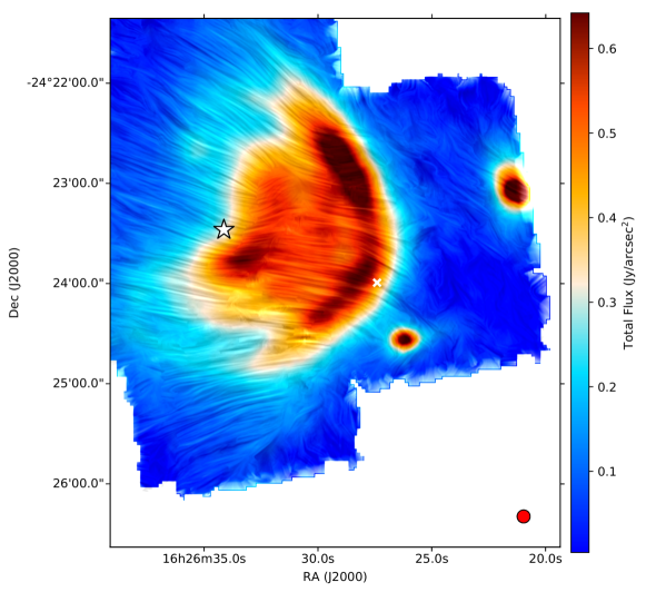
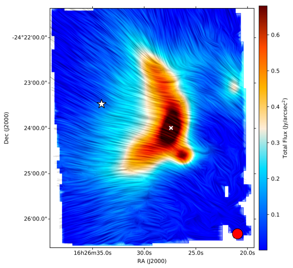
Figure 2: Line-integral-convolution maps of the inferred magnetic field direction in $\rho$ Oph A from bands C (top) and D (bottom). The colors indicate the Stokes I emission in each band. The star indicates the position of Oph S1, and the $\times$ marks the peak column density position. Notice that both maps have the same spatial scale and centering. The circle at the bottom right of each panel represents the beam size (FWHM).

From the polarization angle maps, we have generated maps of magnetic field direction using the standard assumption that the E vector of far-IR polarization is perpendicular to the component of the magnetic field in the plane of the sky (e.g., Lazarian, 2007). The maps of magnetic field direction are visualized using the Line-Integral-Convolution technique (LIC, Cabral & Leedom, 1993) in Figure 2 for bands C (top) and D (bottom). In each map, colors represent total intensity (Stokes I) for the respective band, while the overlaid LIC “texture” represents the inferred sky-projected magnetic field directions obtained from the 90-deg rotated polarization angles.

The total intensity maps for both bands exhibit large arc-shaped features approximately centered on Oph S1. However, a comparison of these two total intensity maps reveals that they have important differences. Presumably, these differences are explained by strong temperature gradients that arise due to the effects of radiation from Oph S1. Band D generally has higher fluxes near the column density peak, preferentially probing the largest column densities. In contrast, the highest fluxes in band C do not correspond to the column density peak, but instead to the warmer areas near Oph S1.

From the LIC maps, we note that, overall, the projected magnetic field is approximately perpendicular to the ridge observed in the column density map of Figure 1. This is in qualitative agreement with ground-based polarimetry at longer wavelengths, as can be seen by comparison with Figure 29 of Dotson et al. (2010) and Figure 5 of Kwon et al. (2018). There is also a general tendency for the magnetic field in the lowest density gas to extend from the Southwest to Northeast direction, as was seen by Kwon et al. (2015) in the near-infrared. However, our data, which probe deeper into the higher density material, see more of a curvature to the field in the immediate vicinity of $\rho$ Oph A itself, with field lines bending perpendicularly to the curved ridge. This effect is seen more markedly in band D, which traces more of the colder material, deeper into the ridge, as compared to band C, which provides a better probe of the warmer material near Oph S1 and in the dense ridge outer layers. This gives us some insight into the way the field changes with depth into the cloud. The band D data most closely resemble the $850\,\mu$m data of Kwon et al. (2018) that trace the coldest, densest material. Hence, we see that our data fill the gap in understanding at intermediate depths between the lowest density material and the highest.

We find a wide spread of polarization degree values (between $0\%$ and $\approx 15\%$), with median values for bands C and D at $7.5\%$ and $5.0\%$, respectively. There is a clear tendency for lower polarization values to be concentrated near the densest portions of the $\rho$ Oph A core, with median polarization values dropping to $5.1\%$ and $1.7\%$ for bands C and D, respectively, when considering only points within $30\arcsec$ of the column density peak. This trend in polarization degree will be further explored in Section 4.

3.2 Column density and dust temperature maps

The H₂ column density ($N$) and temperature ($T$) maps used in this work (Figure 1) were derived from Herschel $70$, $100$ and $160\,\mu$m PACS data (Photodetector Array Camera and Spectrometer, Poglitsch et al., 2010) obtained from the Herschel Science Archive. The $70$ and $100\,\mu$m maps were Gaussian-convolved to the same angular resolution of the $160\,\mu$m data ($11.4\arcsec$ FWHM) and re-gridded to allow a pixel-by-pixel match. A modified thermal Spectral Energy Distribution (SED) fit was applied to each pixel using a fixed dust opacity spectral index of $\beta=1.62$ (Planck Collaboration XI, 2014).

From each fit we obtain the dust temperature $T$ and the optical depth $\tau_{\lambda_{o}}$ at a reference wavelength chosen to be $\lambda_{o}=250\,\mu$m. Following Hildebrand (1983), $\tau_{\lambda_{o}}$ was then converted to H₂ column density ($N$) using the relation $\tau_{250}=\kappa_{250}\,\mu\,m_{\mathrm{H}}\,N$, where $\kappa_{250}=0.1\,$cm²g^-1 is the dust emissivity cross section per unit mass at $250\,\mu$m, $\mu=2.8$ is the mean molecular weight, and $m_{\mathrm{H}}$ is the mass of the hydrogen atom. The inclusion in our fits of more Herschel data at longer wavelengths (e.g., $250$, $350$, and $500\,\mu$m) did not cause a significant change in the values of $T$ and $N$ obtained. Therefore, to preserve angular resolution in the final $N$ and $T$ maps, the results presented here employ only $70$, $100$ and $160\,\mu$m data. It is important to point out that though we have fitted a single modified black-body to each pixel, in reality the total dust emission for any given pixel is comprised of contributions from several components along the line-of-sight (LOS) at different local temperatures. This notion will be further explored in Sections 3.4 and 3.5. In order to avoid confusion between the local temperature and the temperature that is obtained by fitting the emission from a particular LOS, we will use different terms to refer to each of these quantities. The latter quantity will be referred to as the “LOS temperature” or simply “temperature”, while the former quantity will be called the “local temperature”.

3.3 Polarization spectra

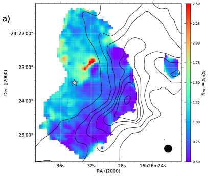
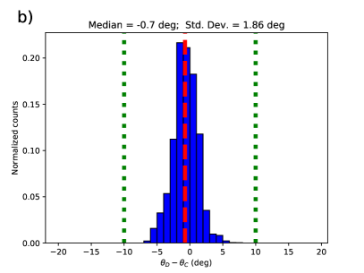
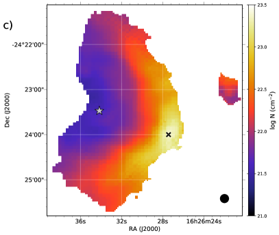
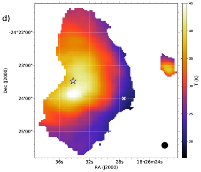
Figure 3: Polarization spectrum analysis of $\rho$ Oph A. (a) Map of $\mathcal{R}_{DC}$$=p_{D}/p_{C}$, with $\mathrm{H}_{2}$ column density ($N$) contour levels distributed between $1\times 10^{22}$ cm^-2 (lower level) and $2\times 10^{23}$ cm^-2 (upper level). (b) Histogram of the polarization angle difference between bands D and C ($\theta_{D}-\theta_{C}$); the red dashed vertical line indicates the median of the distribution ($-0.7^{\circ}$), and the green dotted lines show the $10^{\circ}$ limit as a reference. Panels (c) and (d) show the same $N$ and $T$ maps as in Figure 1, but selecting only the map areas where $\mathcal{R}_{DC}$ data are available (compare with panel (a)) – this is the “polarization spectrum map area”, and it defines the input data used for the cloud core modeling in Section 3.5. The $\times$ symbol indicates the $N$ peak and the gray-colored star symbol indicates the position of Oph S1. The circle at the bottom right of panels (a), (c), and (d) represents the corresponding beam size (FWHM).

To probe the slope of the far-infrared polarization spectrum across $\rho$ Oph A, we define the “polarization ratio” as $\mathcal{R}_{DC}=p_{D}/p_{C}$. With this definition, positive and negative spectrum slopes are indicated by $\mathcal{R}_{DC}>1$ and $\mathcal{R}_{DC}<1$, respectively. The first step in calculating $\mathcal{R}_{DC}$ is to re-generate the band C polarization maps using a merging Gaussian kernel to match the band D beam size ($13.6\arcsec$ FWHM). Next, we calculate $\mathcal{R}_{DC}$ for each sky position. The resulting polarization ratio map is shown in Figure 3a. Typically, investigations of polarization spectra of molecular cloud dust emission employ data masking to reject sky positions having large differences in polarization angles across different wave-bands. A typical threshold would be ten degrees (e.g., for our case, points having $|\theta_{D}-\theta_{C}|>10^{\circ}$ would fail this cut). As can be seen from the histogram in Figure 3b, we see a correlation in polarization angles between bands D and C that is very tight, with no corresponding detections in bands C and D having polarization angle differences larger than $10^{\circ}$. Note that although the bands C and D polarization maps independently cover sky regions well beyond the area shown in Figure 3a, we select for analysis only those sky positions for which polarization detections are available in both bands. We will refer to this ensemble of sky positions as the “polarization spectrum map area.” This same criterion is applied to the column density and temperature maps (see Figures 3c and 3d). Thus, the analysis of column density and temperature presented below will only make use of $N$ and $T$ data located within the polarization spectrum map area.

A clear spatial trend is seen for the polarization ratio across $\rho$ Oph A: North-Eastern regions (including Oph S1) typically show $\mathcal{R}_{DC}$ $>1$, while South-Western regions in general show $\mathcal{R}_{DC}$ $<1$. Interestingly, these trends observed in $\mathcal{R}_{DC}$ can be correlated with trends observed in the column density and temperature maps, which are shown in Figures 3c and 3d, respectively. It appears that lower column density (and warmer) areas are typically associated with a positive polarization spectrum slope ($\mathcal{R}_{DC}$ $>1$). Similarly, as one goes deeper into the cloud (higher column density and colder regions), a negative polarization spectrum slope ($\mathcal{R}_{DC}$ $<1$) becomes predominant. For clarity, column density contours are also included in Figure 3a.

3.4 Qualitative interpretation of the polarization ratio

Let us picture the core of $\rho$ Oph A as a dense structure embedded within a more diffuse molecular cloud, with the latter corresponding to the extended molecular complex generally known as the $\rho$ Ophiuchi cloud. We reserve the term “core” (or “cloud core”) to refer specifically to the denser structure, while the term “ambient” medium will refer to all the material along the LOS immediately outside the core, i.e., the ambient ISM corresponds to the more diffuse molecular cloud material. Finally, the term “cloud” will refer to the combination of the core plus the ambient medium.

As an initial approach to explain the negative (positive) correlation of $\mathcal{R}_{DC}$ with column density $N$ (temperature $T$), we will propose a qualitative picture based on a fall-off in grain alignment efficiency as one goes from the core’s outer edge to its inner higher density regions. As discussed in Section 1, such a fall-off is a prediction of RATs theory as well as being a leading candidate for explaining the widely observed anti-correlation between polarization fraction of emitted radiation and column density. For purposes of the discussion in this Section, we will ignore other explanations for this anti-correlation (but we reconsider this in Section 4.2). It is clear that grains in the core’s more diffuse outer layers are more exposed to UV/optical radiation and therefore are naturally expected to be warmer when compared to those in the shielded high-density core’s interior. In the context of RATs theory, the radiation not only heats the grains, but also increases grains’ efficiency for becoming aligned with respect to the magnetic field. In this case, grains located in the warm outer layers will be well aligned, with the alignment efficiency gradually decreasing towards the core center. From the observational perspective, there is strong evidence from numerous studies that indeed the alignment efficiency seems to decrease at molecular cloud’s interiors (see Section 1). In their most general form, these trends in temperature and grain alignment efficiency have been referred to as the extinction-temperature-alignment correlation (ETAC, Ashton et al., 2018). We will use this term here.

We now argue that the ETAC provides a qualitative explanation for the anti-correlation between $\mathcal{R}_{DC}$ and $N$ that we have observed. First, we introduce the term “core limb” to refer to the sky projection of the core’s outer layers, analogously to the Sun’s limb. Next consider, from the observer’s point of view, how the radiation observed at the core limb LOS differs from that observed for the LOS passing through the core’s center. The core limb LOS can be approximated as a single diffuse and warm component (neglecting for the moment the ambient medium component). On the other hand, the core center LOS includes multiple components (outermost as well as inner core regions) having very different local temperatures and grain alignment efficiencies. For the core center LOS, we have a combination of: (1) well-aligned and warm dust particles in the core’s outer layers, which favors an enhancement of the shorter wavelength polarization, $p_{C}$; with (2) poorly-aligned cold grains in the dense interior, which suppresses the longer wavelength polarized emission, $p_{D}$. This combination should lead to a smaller $\mathcal{R}_{DC}$ value toward the center LOS in comparison with the core limb where we have a single diffuse component with well-aligned warm grains (no ETAC effect). This is precisely the trend we observe in Figure 3a. Note that Hildebrand et al. (1999) were the first to propose this same basic qualitative picture. In that case, the picture served to address the tension between the predicted flat spectra and the observed falling spectra (see discussion in Section 1).

The qualitative scenario described above requires quantitative tests. To this end, as a sanity check on whether the ETAC can be considered a plausible explanation for why $\mathcal{R}_{DC}$ decreases as column density increases, we will now compare our observations with a very crude, very simple toy model in which we assume that the ETAC is the only effect causing changes in grain alignment efficiency. Our model is described in Section 3.5. Note that the very simple model presented here is not intended to correspond to the core of $\rho$ Oph A as a whole. Rather, because it uses only the $N$ and $T$ data located within the polarization spectrum map area (Figures 3c and 3d, respectively), it effectively represents only the Eastern side of the core (which faces Oph S1). This is all we can model, as this is the region for which we obtained corresponding polarization detections for both bands C and D.

3.5 Simple cloud model

3.5.1 Overview of the simple cloud model

The simple cloud model consists of a spherically symmetric core of radius $R$ embedded in a uniform ambient medium (or “background”) with H₂ column density $N_{\mathrm{b}}$ and temperature $T_{\mathrm{b}}$. We set the center of the spherical core to be located at the peak of the column density map (as indicated by the $\times$ symbol in Figures 3c and 3d). The core’s H₂ number density profile is described by a Plummer sphere: $n(r)=n_{o}/(1+r^{2}/R_{\mathrm{p}}^{2})^{5/2}$, where $r$ is the distance from the center, $n_{o}$ is the H₂ number density at the center, and $R_{\mathrm{p}}$ is the Plummer radius. Similar density profiles (e.g., Plummer and “Plummer-like”) are frequently used to describe molecular filaments (e.g., Nutter et al., 2008; Arzoumanian et al., 2011) and molecular cores (e.g., Whitworth & Ward-Thompson, 2001; Whitworth & Bate, 2002). For simplicity, the local temperature profile $T(r)$ is assumed to vary linearly between the core’s center (where $T(0)=T_{o}$) and its edge ($T(R)=T_{R})$. A schematic representation of the simple model, including the parameters described above, is shown in Figure 4. In the following analysis, we define $x$ to be the projected distance from the core center in the plane of the sky (assuming a cloud distance of $137\,$pc).

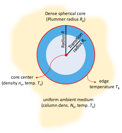
Figure 4: Schematic representation of the simple cloud model described in Section 3.5. The seven parameters $R$, $N_{\mathrm{b}}$, $T_{\mathrm{b}}$, $n_{o}$, $R_{\mathrm{p}}$, $T_{o}$, and $T_{R}$ are found by using the column density and temperature maps derived from Herschel (Section 3.2), as described in Sections 3.5.1 and 3.5.2. The transition radius $R_{t}$, described in Section 3.5.3, is introduced to test the hypothesis that grain alignment efficiency decreases toward the core center (i.e., the ETAC hypothesis): for $r<R_{t}$, the model assumes that grain particles are completely unaligned.

The seven parameters $R$, $N_{\mathrm{b}}$, $T_{\mathrm{b}}$, $n_{o}$, $R_{\mathrm{p}}$, $T_{o}$, and $T_{R}$ completely specify the wavelength-dependent total-intensity distributions in our model cloud. Our strategy here is to first use the column density and temperature maps derived from Herschel (see Section 3.2) to determine these seven parameters before proceeding to consider grain alignment, polarization, and the HAWC+ data. Since the seven parameters will depend directly on the $N$ and $T$ values derived from Herschel, it is important to note that these $N$ and $T$ values carry an intrinsic uncertainty related to the measurement errors and the inaccuracies in the technique employed in Section 3.2.

Here is a step-by-step overview of our method:

• Step 1: From the Herschel $N$ and $T$ maps, we determine “median NT curves” that represent the input column density ($N$) and temperature ($T$) data as a function of $x$, the projected distance from the core center. Using these curves we determine the core radius $R$ and the ambient medium parameters $N_{\mathrm{b}}$ and $T_{\mathrm{b}}$.

• Step 2: We compute ambient-subtracted column density and temperature maps, allowing us to determine the local temperature at the core edge ($T_{R}$).

• Step 3: We conduct a “simulated observation” of the simple model core + ambient medium, calculating “output NT curves” that can be compared to the median NT curves. This procedure involves a flux integration along the LOS through the model cloud. The three remaining input parameters ($n_{o}$, $R_{\mathrm{p}}$, $T_{o}$) are determined by minimizing the difference between the output NT curves and the median NT curves.

• Step 4: We adopt a simple prescription for the dependence of grain alignment on core depth, and then integrate the polarized fluxes along the LOS. This allows us to estimate model curves of polarization degree (in bands C and D) and $\mathcal{R}_{DC}$ as functions of column density, which can be directly compared with the polarimetric observations.

Steps 1, 2, and 3 above are described in detail in Section 3.5.2, while Step 4 is elaborated in Section 3.5.3.

3.5.2 Fixing the simple cloud model total intensity parameters

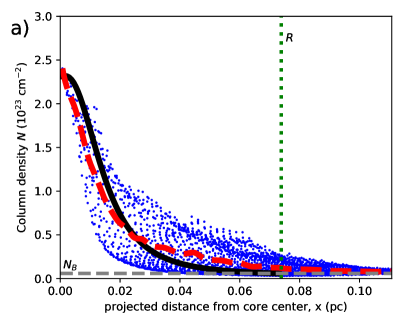
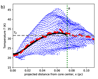
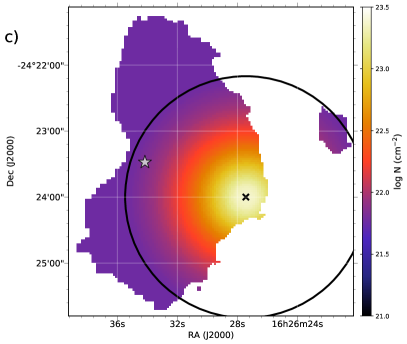
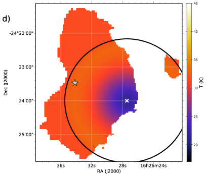
Figure 5: Spherical cloud core modeling of $\rho$ Oph A. Panels (a) and (b) show the $N$ and $T$ projected distance distributions (blue points), using data shown in Figure 3c and d, respectively. The red dashed lines are median NT curves using the blue points as inputs. The solid black lines are the model outputs for column density and dust temperature after integrating the fluxes along the LOS and simulating an observation of the spherical core (see Section 3.5.2). Gray horizontal dashed lines in panels (a) and (b) represent the column density ($N_{\mathrm{b}}$) and temperature ($T_{\mathrm{b}}$) of the model uniform ambient medium, respectively. Green vertical lines represent the core radius $R$. Mapping representations of the spherical core model (including the uniform ambient ISM) are shown in panels (c) (column density) and (d) (temperature). The $\times$ symbol and the solid circle represent the center of the core and the core radius $R$, respectively. The star symbol in panels (c) and (d) shows the corresponding position of Oph S1, and is given here just for reference to compare with Figure 3.

The determination of the seven total-intensity parameters for the simple model, following the steps listed in Section 3.5.1, is carried out as follows: First (Step 1 of Section 3.5.1), we use the column density and temperature maps to build projected distance distributions of $N$ and $T$, which are shown as blue points in Figures 5a and b, respectively. As mentioned above (Section 3.3), in these projected distance distributions we include only data located within the polarization spectrum map area (these data are shown in Figures 3c and 3d, respectively). For both the $N$ and $T$ distributions as a function of $x$, median-binned curves are computed. These are shown using red-dashed lines in 5a and b. These curves are referred to as the “median NT curves” and are denoted as $\overline{N}(x)$ and $\overline{T}(x)$. The goal is to find values for the seven total intensity parameters that reproduce these median NT curves as closely as possible.

We start by setting the limb of the model spherical core to be located at the point where $\overline{N}(x)$ falls to 5% of its peak value. This gives $R=0.074\,$pc. To find $N_{\mathrm{b}}$ and $T_{\mathrm{b}}$, respectively, we take the median of all $N$ and $T$ values at $x>R$, restricting to the polarization spectrum map area. The maximum $x$ value in this area is $1.72R$, so $N_{\mathrm{b}}$ and $T_{\mathrm{b}}$ provide suitable estimates of the ambient column density and temperature immediately outside the cloud core: $N_{\mathrm{b}}=5.7\times 10^{21}\,$cm^-2 and $T_{\mathrm{b}}=30.7\,$K. The 5% choice described above for setting $R$ corresponds to $\overline{N}(R)$ just 1$\sigma$ larger than $N_{\mathrm{b}}$, where $\sigma$ is the standard deviation of the distribution of column density values for $x>R$, which is a measure of the variation of the background column density that has a mean value of $N_{\mathrm{b}}$. (The numerical value of $\sigma$ is $5.0\times 10^{21}\,$cm^-2.) Thus, this 5% choice appropriately limits the model core to a region where core emission can be reasonably distinguished from background emission.

Keeping in mind that we now have four remaining total intensity parameters, $n_{o}$, $R_{\mathrm{p}}$, $T_{o}$, and $T_{R}$, we move to Step 2 of Section 3.5.1. We find that one of these parameters, $T_{R}$, can be directly inferred from the Herschel-derived temperature map in a straightforward way. This is because, from the observer’s perspective, the core limb LOS involves the superposition of only two cloud components: the uniform ambient medium and the layer of the core for which $r=R$. Accordingly, from $N_{\mathrm{b}}$ and $T_{\mathrm{b}}$ we compute the ambient ISM flux values $I_{\lambda,b}$ for each Herschel wavelength $\lambda$, using the same modified blackbody SED and scaling relations described in Section 3.2. We then remove this ambient contribution by subtracting these wavelength-dependent flux values from each Herschel map. Next, we compute ambient-subtracted column density and temperature maps using a procedure identical to the one described in Section 3.2. From the ambient-subtracted temperature map, we find $T_{R}=38.9\,$K by taking the median temperature value at $x=R$. For completeness, we note that the median ambient-subtracted column density at $x=R$ is $2.0\times 10^{21}\,$cm^-2.

A key ingredient in our method for setting the values for the last three parameters (Step 3 of Section 3.5.1) is our procedure for conducting a “simulated Herschel observation” of the model cloud, yielding column density and temperature profiles (“output NT curves”) that can be compared to the median NT curves ($\overline{N}(x)$ and $\overline{T}(x)$) of Figures 5a and b. First, we choose 100 values of $x$ that are uniformly distributed between $x=0$ and $x=R$, and then for each combination of one of these $x$ values and one choice of Herschel-band, we integrate the Herschel-band emission at each core radius $r$ along the line-of-sight to find the flux $I_{\lambda}(x)$:

$$I_{\lambda}(x)=\kappa_{250}\,\mu\,m_{\mathrm{H}}\,\left(\frac{\lambda_{o}}{\lambda}\right)^{\beta}\int n(r)\,B_{\lambda}(T(r))\,ds+I_{\lambda,b}$$ (1)

In the expression above, $\lambda$ is the wavelength corresponding to the Herschel-band, $s$ represents distance along the LOS, $B_{\lambda}$ is the Planck function, and the parameters $\kappa_{250}$, $\mu$, $m_{\mathrm{H}}$, and $\beta$ were defined in Section 3.2. Notice that, in contrast with our earlier treatment that is valid for arbitrary optical depth (Section 3.2), Equation 1 relies on the optically thin approximation. As discussed in Section 4.3, this introduces only a modest level of error in the final calculated polarization ratios.

Secondly, we use the simulated observed fluxes $I_{\lambda}(x)$ to compute model column density $N_{m}(x)$ and temperature $T_{m}(x)$ values for each value of $x$, using the procedure described in Section 3.2 (i.e., fitting a modified black-body function to the fluxes). Obviously this entire “simulated observation” procedure requires values for all seven total intensity parameters, including the three that have until now remained unconstrained ($n_{o}$, $R_{\mathrm{p}}$, and $T_{o}$). For a given set of parameters, we can compute curves of $N_{m}(x)$ and $T_{m}(x)$ (as exemplified in Figures 5a and 5b by the thick black curves), and compare them to the curves of $\overline{N}(x)$ and $\overline{T}(x)$ (red-dashed lines in the same figures).

To determine the best values for $n_{o}$, $R_{\mathrm{p}}$, and $T_{o}$, we ran the simulated model observation multiple times, varying these three parameters in each run, and searched for the set that minimizes the difference between the output NT curves ($N_{m}(x)$ and $T_{m}(x)$) and the median NT curves ($\overline{N}(x)$ and $\overline{T}(x)$). For each run, we calculated the quantity $\Delta_{NT}=\sum_{x}(N_{m}(x)-\overline{N}(x))^{2}\times\sum_{x}(T_{m}(x)-\overline{T}(x))^{2}$, which can be understood as the combined summed square difference between the column density and temperature curves. The quantity $\Delta_{NT}$ was minimized for the following best-fit values: $n_{o}=6.4\times 10^{6}\,$cm^-3, $R_{\mathrm{p}}=0.244\,R$, and $T_{o}=13.9\,\mathrm{K}$. The adopted values for all seven total intensity parameters are collected in Table 1. The thick black curves in Figures 5a and b show $N_{m}(x)$ and $T_{m}(x)$ as computed from these adopted parameters.

Table 1: Parameters of the simple spherically symmetric cloud-core model

Parameter	Description	Determined value
$R$	Core radius	$0.074\,$pc
$N_{\mathrm{b}}$	H2 ambient column density	$5.7\times 10^{21}\,$cm-2
$T_{\mathrm{b}}$	Ambient dust temperature	$30.7\,$K
$T_{R}$	Local dust temperature at the core edge ($r=R$)	$38.9\,$K
$n_{o}$	H2 number density at the core center ($r=0$)	$6.4\times 10^{6}\,$ cm-3
$R_{\mathrm{p}}$	Core Plummer radius	$0.244\,R$
$T_{o}$	Local dust temperature at the core center ($r=0$)	$13.9\,\mathrm{K}$
$R_{t}$	Polarization transition radius	$0.6\,R$

Lastly, using these final $N_{m}(x)$ and $T_{m}(x)$ curves, Figures 5c and d show map representations of the column density and temperature profiles, respectively, for our simple model. Given the limitations of our spherical-core approximation for $\rho$ Oph A, these maps provide something close to the best possible representation of the real cloud based on the simple model and the inputs from the Herschel observations. Comparing Figures 3c and d with Figures 5c and d, we note that some of the very general features of the column density and temperature maps are well reproduced by the simple model, e.g., the low temperatures and high column densities near the core center, as well as the lower column densities and warmer temperatures surrounding the core. However, there are many obvious differences between the real and model maps. Our simple approach provides for an initial sanity check (as discussed in Section 3.4 and also below), but in Section 4.3 we discuss ways in which the model could be improved in future investigations.

3.5.3 Polarization degree and polarization ratio for the simple cloud model

In the paradigm described in Section 3.4, based on ETAC, dust grains have gradually decreasing alignment efficiency going from the diffuse outskirts of the core towards its dense interior. For the purpose of the very simple toy model developed in this work, we choose the simplest grain alignment prescription that is consistent with ETAC: we assume that at very high densities, interior to a certain cutoff radius, dust grains are completely unaligned, so that the polarization detected toward the central parts of the dense core actually originates in the core’s more diffuse outer layers (i.e., there is no internal heating from embedded sources). Accordingly, we define a cutoff “transition radius” $R_{t}$ interior to which the alignment efficiency is set to zero. Given this assumption, the goal here is to calculate the expected values of $\mathcal{R}_{DC}$ from the model cloud, in order to compare with the observations (following Step 4 described in Section 3.5.1). For each sky-projected distance $x$ from the core center, we use the definition of polarization degree: $p_{\lambda}(x)=P_{\lambda}(x)/I_{\lambda}(x)$, where $P_{\lambda}(x)$ is the polarized flux (see below) and $I_{\lambda}(x)$ is the total flux (e.g., as might be computed using Equation 1). To account for the effect of a cutoff radius for the polarization efficiency, we calculate the polarized flux according to the following prescription:

$$P_{\lambda}(x)=p_{\lambda,o}I^{\prime}_{\lambda}(x)\ ,$$ (2)

where $I^{\prime}_{\lambda}(x)$ is calculated as in Equation 1, but excluding the region between $s=-\sqrt{R_{t}^{2}-x^{2}}$ and $s=+\sqrt{R_{t}^{2}-x^{2}}$ from the integral. Parameter $p_{\lambda,o}$ represents the ambient polarization efficiency outside the volume defined by the transition radius. For simplicity, it is assumed to be spatially uniform. For each band, $p_{\lambda,o}$ is found by taking the median polarization degree for all polarization detections within the polarization spectra map area having $x>R_{t}$.

Using this simple model, we calculate the values of polarization degree in bands D and C as a function of $x$: $p_{D,m}(x)$ and $p_{C,m}(x)$, respectively. In addition, the model polarization ratio $\mathcal{R}_{DC,m}$$(x)=p_{D,m}(x)/p_{C,m}(x)$ is computed. By combining with the $N_{m}(x)$ and $T_{m}(x)$ curves obtained in Section 3.5.2, we can find model-estimated curves of any of $p_{D,m}$, $p_{C,m}$ and $\mathcal{R}_{DC,m}$ as a function of either column density $N_{m}$ or temperature $T_{m}$.

Note that this simple polarization model for the cloud has only one free parameter, the transition radius $R_{t}$. For the purpose of this analysis we have chosen three values: $R_{t}=0.3\,R$, $0.6\,R$, and $0.9\,R$ (these values were selected since they encapsulate the full parameter space of the observations, which we will describe in more detail in Section 4.2). Comparisons between observed and model curves of polarization degree and polarization ratio are shown in Figure 6. In each panel of Figure 6, the yellow-blue-red colored background represents 2D histograms of the HAWC+ observations: $p_{C}$ vs. $\log{N}$ in panel (a), $p_{D}$ vs. $\log{N}$ in panel (b), $\mathcal{R}_{DC}$ vs. $\log{N}$ in panel (c), and $\mathcal{R}_{DC}$ vs. $T$ in panel (d). The colored curves represent the model $p_{C,m}$, $p_{D,m}$ and $\mathcal{R}_{DC,m}$ as a function of $\log{N_{m}}$ (Figures 6a, 6b, and 6c, respectively) and $\mathcal{R}_{DC,m}$ as a function of $T_{m}$ (Figure 6d) using the three chosen values of $R_{t}$, as explained above. These graphs are interpreted and discussed in Section 4.

4 Discussion

4.1 Comparison between the observed far-IR polarization spectrum
and physical dust model predictions

The $\mathcal{R}_{DC}$ map presented in Section 3.3 suggests correlations of the polarization spectrum slope with column density $N$. In the 2D histogram of the observed $\mathcal{R}_{DC}$ as a function of column density (Figure 6c), such a correlation is clearly seen: $\mathcal{R}_{DC}$ goes from $>1$ to $<1$ as $N$ increases. Given that $N$ and $T$ are highly anti-correlated within the polarization spectrum map area (compare Figures 3c and 3d) a correlation of $\mathcal{R}_{DC}$ with $T$ is also expected. In fact, viewing $\mathcal{R}_{DC}$ as a function of temperature (Figure 6d), $\mathcal{R}_{DC}$ changes from $<1$ to $>1$ as $T$ increases. Previous observations of the far-infrared polarization spectrum toward star-forming clouds have detected negative polarization spectrum slopes (Vaillancourt, 2002; Vaillancourt et al., 2008; Vaillancourt & Matthews, 2012; Zeng et al., 2013), but no clear systematic dependence on column density (or temperature) has been reported previously. In particular, the positive polarization spectrum slopes we observe toward the more diffuse areas surrounding the core provide a connection with the grain alignment models of Bethell et al. (2007), Draine & Fraisse (2009), and Guillet et al. (2018), all of which predict positive slopes for this wavelength range.

An approximate quantitative comparison between the positive polarization spectrum slopes observed toward $\rho$ Oph A and the predicted $\mathcal{R}_{DC}$ values from the models available in the literature can be made. For instance, although the modeled polarization spectra from Bethell et al. (2007) is averaged over a wide range of column densities, their mean $N$ value lies between $\approx 10^{21.5}\,$cm^-2 and $\approx 10^{22.0}\,$cm^-2. This range is similar to the lower column density coverage of the HAWC+ observations toward $\rho$ Oph A (see Figure 6c). For $\rho$ Oph A, we find a mean $\mathcal{R}_{DC}$ value of $1.1$ within this same range of column densities. From the models by Bethell et al. (2007), we estimate predicted $\mathcal{R}_{DC}$ values between $1.75$ and $2.0$ based on their Figure 13. Notice, however, that the dust temperatures assumed by Bethell et al. (2007) (in the range $\approx 5-17\,$K) are significantly colder than the temperatures in the positive-slope polarization spectrum region of $\rho$ Oph A (between $\approx 30\,$K and $\approx 45\,$K, near Oph S1 – see Figure 3d).

Guillet et al. (2018) also presented predicted polarization spectrum curves ($p$ vs. $\lambda$), although for a somewhat lower column density regime, between $\approx 10^{21.0}\,$cm^-2 and $\approx 10^{21.5}\,$cm^-2 (translucent clouds). They point out that there is a strong correlation between the dust temperature and the intensity of the interstellar radiation field (ISRF). Moreover, as shown by their Figure 15, the polarization spectrum curves are significantly affected by the ISRF level. In the range of models presented by Guillet et al. (2018) with different ISRF intensities, the ones with higher ISRF levels show $\mathcal{R}_{DC}$$\,\approx 1.1$, while models with lower ISRF intensities show $\mathcal{R}_{DC}$$\,\approx 20.0$. This suggests that the $\mathcal{R}_{DC}$ parameter within the lower column density regime is expected to be significantly affected by the level of exposure to radiation (and consequently, by the dust temperature). Given the proximity of the lower-density positive-slope regions of $\rho$ Oph A to Oph S1, it is plausible to speculate that the somewhat lower $\mathcal{R}_{DC}$ values as compared to the models might be due to the strong exposure to radiation (and warmer dust temperatures) in this area. A more accurate comparison between models and observations of the far-IR polarization spectrum slope for lower density regimes requires an accurate treatment of the ISRF, which is beyond the scope of this work. For completeness, it is worth pointing out that although the Draine & Fraisse (2009) models probe a very different regime (the diffuse ISM), they predict $\mathcal{R}_{DC}$ values between $1.4$ and $2.6$, which are also slightly higher than the mean values found in $\rho$ Oph A for the lower column density areas.

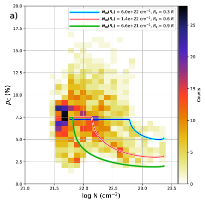
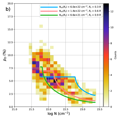
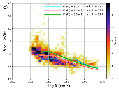
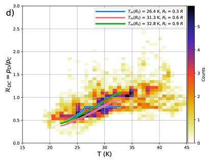
Figure 6: Comparison of the HAWC+ polarization data (colored 2D histograms), with the predictions of the simple cloud model of $\rho$ Oph A (colored curves): (a) $p_{D}$ vs. $\log N$; (b) $p_{C}$ vs. $\log N$; (c) $\mathcal{R}_{DC}$ $=p_{D}/p_{C}$ vs. $\log N$; (d) $\mathcal{R}_{DC}$ $=p_{D}/p_{C}$ vs. $T$. The blue, red and green solid lines represent three choices of the transition radius $R_{t}$: $0.3R$, $0.6R$, and $0.9R$, respectively. The legends in each panel indicate the model column densities (panels a, b, and c) and model LOS temperatures (panel d) associated with each of these $R_{t}$ values.

4.2 Analysis of the results from the simple spherical cloud model of $\rho$ Oph A

The correlations between $\mathcal{R}_{DC}$ and the column density, found in the observational data, motivated the development of our simple cloud model with the goal of investigating whether ETAC can explain the correlations or not. Below we discuss the comparison between the observational data and the curves generated from this simple model (see Figure 6). In Figures 6a and 6b, the observations exhibit a decrease of polarization degree as column density increases. This trend is commonly observed in molecular clouds (Goodman et al., 1995; Gerakines et al., 1995; Matthews et al., 2002; Whittet et al., 2008; Chapman et al., 2011; Cashman & Clemens, 2014; Alves et al., 2014; Jones et al., 2015; Fissel et al., 2016). Similarly, the simple model curves shown in blue, red, and green also exhibit a decreasing trend in the $p$ vs. $N$ graphs (Figures 6a and 6b). As noted above, we have chosen a set of three values for the free parameter $R_{t}$: $0.3\,R$, $0.6\,R$, and $0.9\,R$. The reason for these particular choices is that the extreme values ($0.3\,R$ and $0.9\,R$, green and blue curves, respectively) represent an approximate “boundary” for the spread in the observational data points of Figure 6 panels (a) and (b). Therefore, choices outside this range are probably poor fits to the data. In this sense the midpoint choice ($R_{t}=0.6\,R$, red line, and also given in Table 1) is a reasonable best fit to the observed dependence of $p_{C}$ and $p_{D}$ on $N$. Note that we can directly associate each value of the transition radius with a corresponding column density $N_{m}(R_{t})$ along the LOS. For $R_{t}=0.6\,R$ we find $N_{m}(R_{t})=1.4\times 10^{22}\,$cm^-2. For column densities larger than this value, grains are no longer aligned.

Within the range of column densities probed in the polarization spectrum map area (between $\approx 10^{21.5}\,$cm^-2 and $\approx 10^{23.4}\,$cm^-2), we detect a change in $\mathcal{R}_{DC}$ from $\approx 1.2$ to $\approx 0.6$ (i.e., approximately a factor of two). In Figure 6c, although the colored model curves do not go through the bulk of the data points, it can be seen that the change in $\mathcal{R}_{DC}$ expected from the models (approximately a factor of 1.5 to 2.0) is similar to the change seen in the observations. Keeping in mind that the seven total intensity parameters were set by considering only the column densities and temperatures derived from Herschel maps of the real cloud (see Section 3.5.2), and that $R_{t}$, the sole remaining parameter that can affect how much $\mathcal{R}_{DC}$ varies with column density, was also set without any reference to the observed values of $\mathcal{R}_{DC}$ (see Section 3.5.3), it seems surprising that our simple cloud model can reproduce the general trends seen in the $\mathcal{R}_{DC}$ observations as well as it does. We conclude that a simple cloud model which takes into account only ETAC can reasonably reproduce the observed systematic changes of the far-infrared polarization spectrum slope within the studied range of column densities. This result is consistent with the RATs explanation for the observed changes in the polarization spectrum. It is important to note, however, that an increased degree of magnetic field disorder deep inside the core provides an alternative way to obtain lower levels of polarization for light emitted from the densest central regions of a core. We cannot discard this as an explanation for all or part of the trend we have discovered, even if the near-infrared spectro-polarimetry results discussed in Section 1 suggest that in fact changes in grain alignment do play the dominant role. Disentangling field disorder from the expected loss of grain alignment due to RATs is a difficult problem that is perhaps best tackled with the help of MHD simulations (e.g., see King et al., 2018).

In the context of the ETAC interpretation that is based on RATs theory, the local temperature can be thought of as a proxy for the local intensity of the optical/near-IR radiation field and thus directly related to the dust grain alignment efficiency. Therefore, complementary to the above analysis of $\mathcal{R}_{DC}$ as a function of $N$, it is also instructive to compare the observed relation of $\mathcal{R}_{DC}$ vs. temperature $T$ with the corresponding simple model curves (Figure 6d). The observed increase in $\mathcal{R}_{DC}$ with temperature is clearly well reproduced by the model curves. Note that the temperature plotted in this figure is the LOS temperature rather than the local temperature (see Section 3.2). We can associate each value of the transition radius $R_{t}$ with a corresponding LOS temperature $T_{m}(R_{t})$. For instance, we find $T_{m}(R_{t})=31.3\,$K for $R_{t}=0.6\,R$. However, since it is the local temperature rather than the LOS temperature that serves as the better proxy for the local grain alignment efficiency, we can instead consider the local temperature $T_{l,m}(R_{t})$ corresponding to the transition radius $R_{t}$. For $R_{t}=0.3\,R$, $0.6\,R$, and $0.9\,R$, we find $T_{l,m}(R_{t})$ values of $21.4\,$K, $29.0\,$K, and $36.5\,$K, respectively. It would be interesting to test, by applying a similar analysis to other cores of high column density, whether a critical local temperature lying within this range is universal for high column density cores.

Note that we are not arguing here that high grain temperature is directly responsible for grain alignment. Indeed, there is evidence against this. Specifically, Globule 2 in the Southern Coalsack exhibits efficient grain alignment (Jones et al., 1984) despite its low temperature of $\approx 10\,$K. In the context of RATs theory, this may be attributed to the low column density of about $10^{22}\,$cm^-2, not enough to shield the cloud from the interstellar radiation field (Andersson et al., 2015). By way of comparison, we note that the peak column density in $\rho$ Oph A is larger than $10^{23}\,$cm^-2. Rather than arguing that grain temperature is directly related to grain alignment, we are instead suggesting that in $\rho$ Oph A (and perhaps in other very dense cores) local temperature can serve as a proxy for the radiation intensity, and can thereby be related to grain alignment efficiency.

The results presented in this paper introduce a new method to probe the grain alignment efficiency in molecular clouds, based on trends in the slope of the far-IR polarization spectrum. Provided a model is given for the studied cloud, one may test beyond which core depth, or below which local temperature, the grain alignment is no longer efficient. The usage of the polarization ratio as opposed to the polarization degree itself (as has been done for various previous studies in the literature) offers an advantage, because the polarization degree is affected by inclination of the magnetic field lines with respect to the LOS, whereas the polarization ratio is not. This could explain why the trends in the observed relations of $p_{C}$ and $p_{D}$ as functions of $N$ (Figures 6a and 6b, respectively) are more complicated than the trends observed in $\mathcal{R}_{DC}$ vs. $N$ (Figure 6c). For instance, both $p_{C}$ and $p_{D}$ show a clear decrease as a function of $N$ in the range $22.0<\log{N}\,(\mathrm{cm}^{-2})<23.5$, However, for $\log{N}\,(\mathrm{cm}^{-2})<22.0$, there is a wide spread in the values of $p_{C}$ and $p_{D}$, and the trend is no longer clear. This feature could potentially be due to changes in the magnetic field inclination along the LOS. The trends in $\mathcal{R}_{DC}$ are more clearly represented by a simple monotonic decrease as a function of $N$ (Figure 6c) over the full range of column densities probed by these observations. The polarization degree is also affected by unresolved field structure in the plane-of-the sky, an effect that is also cancelled when using the polarization ratio. In the context of studying the role of the magnetic field in star formation, developing new tools to probe grain alignment efficiency is critical for interpreting interstellar polarization measurements arising from molecular cloud cores and filaments.

4.3 Limitations of the simple spherical cloud model and comparison with longer wavelength polarimetry of $\rho$ Oph A

In this initial work, we have used a very simple approach to model the cloud, but differences between the model and the real cloud are obvious when comparing column density and temperature maps (e.g., compare Figures 3c and 3d to Figures 5c and 5d). There are numerous ways in which this model could be made more realistic, potentially improving the comparison between the model $\mathcal{R}_{DC}$ curves and the polarimetric observations. The most obvious improvement would be to abandon spherical symmetry, adopting a more complicated model tailored to the real cloud. Another way to add significant realism would be to introduce a gradual “turn off” of the grain alignment efficiency as one moves deeper into the core, rather than using our strict cutoff at $r=R_{t}$. In addition, the number density profile (Plummer sphere) and the local temperature profile (linear) could be modified to match the Herschel data more accurately. Finally, although the entire map shows far-infrared optical depth values less than unity, for the densest lines-of-sight this parameter reaches values high enough to invalidate the optically thin approximation used in Equation 1. For instance, at the peak column density of $\rho$ Oph A we estimate optical depths of 0.53 and 0.21 for bands C and D, respectively. This could represent a difference of up to 20% in $\mathcal{R}_{DC}$ at the peak column density, relative to the optically thin situation (see, for example, Novak et al., 1989).

Another extension of the work described here would be to expand the analysis to cover a wider wavelength range, including the $\rho$ Oph A POL-2 data at $850\,\mu$m (Kwon et al., 2018). This should be approached carefully as the HAWC+ and POL-2 datasets likely probe very different column density regimes. In the context of the simple spherical core model presented in this work, this can be verified by analyzing how the integrand of Equation 1 (i.e., the dust emission per unit volume) varies as a function of the LOS depth $s$ toward the core center (i.e., for sightline $x=0$). The HAWC+ dust emission in bands C and D peaks in the range $0.13R-0.26R$ while the $850\,\mu$m dust emission peaks at a significantly deeper core layer, near $0.04R$. This shows that POL-2 probably probes much closer to the cold core center relative to HAWC+ bands C and D. It seems unlikely that the simple sharp cutoff grain alignment prescription used here could capture the physical effects operating over such a large range of core depths. The investigation of the polarization spectrum over a wider range of wavelengths, probably using a more sophisticated grain alignment prescription, is likely to prove informative, but such a study is beyond the scope of the present investigation.

Finally, we note that after the present work was submitted for publication, we became aware of a recent publication by Pattle et al. (2019), who used the same POL-2 data from Kwon et al. (2018) to study the grain alignment efficiency in several dense regions within $\rho$ Ophiuchi, including $\rho$ Oph A. Similarly to our work, their results highlight the importance of the incident radiation field for efficient alignment of dust grains.

5 Summary and Conclusions

In this work we analyzed far-infrared polarimetric data from HAWC+/SOFIA in bands C ($89\,\mu$m) and D ($154\,\mu$m) for the densest portion of $\rho$ Ophiuchi (known as $\rho$ Oph A). The main goal was to evaluate the changes in the slope of the polarization spectrum correlated with local cloud properties (more specifically, column densities and dust temperatures). From previous molecular cloud surveys of the far-infrared polarization spectrum, the slopes were typically found to be negative in this same spectral range (Vaillancourt, 2002; Vaillancourt et al., 2008; Vaillancourt & Matthews, 2012; Zeng et al., 2013). No systematic correlation between far-infrared polarization spectrum and cloud properties has been previously reported.

We defined the polarization ratio $\mathcal{R}_{DC}$ = $p_{D}/p_{C}$ and investigated its distribution across $\rho$ Oph A. The polarization angles in bands C and D are very tightly correlated, which allowed the use of data for all sky positions for which measurements were available at both bands. The polarization ratio map covers the surroundings of the massive star Oph S1, and also includes the peak density at the cloud core. We noticed a clear correlation of $\mathcal{R}_{DC}$ with $N$ and $T$: in the range of column densities and temperatures covered by our dataset (approximately $2.8\times 10^{21}\,\mathrm{cm}^{-2}<N<2.5\times 10^{23}\,\mathrm{cm}^{-2}$ and $20\,\mathrm{K}<T<45\,\mathrm{K}$), $\mathcal{R}_{DC}$ decreases from $\approx 1.2$ (positive polarization spectrum slope) in the more diffuse portions of the core to approximately $0.6$ at the density peak (negative slope). The discovery of positive polarization spectrum slopes is consistent with published dust grain models (Bethell et al., 2007; Draine & Fraisse, 2009; Guillet et al., 2018).

We explain the dependence of $\mathcal{R}_{DC}$ on $N$ and $T$ as a consequence of the ETAC, i.e., grains in the warm and diffuse outskirts of the core are well aligned due to better exposure to radiation, while the alignment efficiency gradually decreases toward the colder and denser shielded core. For the purpose of providing a sanity check on whether the ETAC can quantitatively explain the magnitude of the observed change in $\mathcal{R}_{DC}$, we developed a very simple toy model for $\rho$ Oph A. We model the cloud as a spherically symmetric core embedded in a uniform ambient medium, and we determine the seven model parameters that determine the wavelength-dependent total intensity distributions using Herschel-derived column density and temperature maps. We assume the simplest possible grain alignment efficiency profile, i.e., the alignment is completely turned off interior to a certain radius from the core center. A range of values for cutoff radius is chosen based on the observed dependencies of $p_{D}$ and $p_{C}$ on $N$. Finally, we compare the model’s predictions for $\mathcal{R}_{DC}$ with the observed values, finding rough agreement. Based on this sanity check, we conclude that ETAC appears to be a plausible explanation for the polarization ratio trends observed. We propose that the analysis of far-infrared polarization spectra can be used as a new method to probe the loss of grain alignment within dense interstellar cores.

References

- Alves et al. (2014) Alves, F. O., Frau, P., Girart, J. M., et al. 2014, A&A, 569, L1
- Andersson et al. (2015) Andersson, B.-G., Lazarian, A., & Vaillancourt, J. E. 2015, ARA&A, 53, 501
- Andersson et al. (2011) Andersson, B.-G., Pintado, O., Potter, S. B., Straižys, V., & Charcos-Llorens, M. 2011, A&A, 534, A19
- Andersson & Potter (2010) Andersson, B.-G. & Potter, S. B. 2010, ApJ, 720, 1045
- Andre et al. (1988) Andre, P., Montmerle, T., Feigelson, E. D., Stine, P. C., & Klein, K.-L. 1988, ApJ, 335, 940
- Arce et al. (1998) Arce, H. G., Goodman, A. A., Bastien, P., Manset, N., & Sumner, M. 1998, ApJ, 499, L93
- Arzoumanian et al. (2011) Arzoumanian, D., André, P., Didelon, P., et al. 2011, A&A, 529, L6
- Ashton et al. (2018) Ashton, P. C., Ade, P. A. R., Angilè, F. E., et al. 2018, ApJ, 857, 10
- Astropy Collaboration et al. (2013) Astropy Collaboration, Robitaille, T. P., Tollerud, E. J., et al. 2013, A&A, 558, A33
- Bethell et al. (2007) Bethell, T. J., Chepurnov, A., Lazarian, A., & Kim, J. 2007, ApJ, 663, 1055
- Cabral & Leedom (1993) Cabral, B. & Leedom, L. C. 1993, in Proceedings of the 20th Annual Conference on Computer Graphics and Interactive Techniques, SIGGRAPH ’93 (New York, NY, USA: ACM), 263–270
- Cashman & Clemens (2014) Cashman, L. R. & Clemens, D. P. 2014, ApJ, 793, 126
- Chapman et al. (2011) Chapman, N. L., Goldsmith, P. F., Pineda, J. L., et al. 2011, ApJ, 741, 21
- Chiar et al. (2006) Chiar, J. E., Adamson, A. J., Whittet, D. C. B., et al. 2006, ApJ, 651, 268
- Chuss et al. (2019) Chuss, D. T., Andersson, B. G., Bally, J., et al. 2019, ApJ, 872, 187
- Dolginov & Mitrofanov (1976) Dolginov, A. Z. & Mitrofanov, I. G. 1976, Ap&SS, 43, 291
- Dotson et al. (2010) Dotson, J. L., Vaillancourt, J. E., Kirby, L., et al. 2010, ApJS, 186, 406
- Dowell et al. (2010) Dowell, C. D., Cook, B. T., Harper, D. A., et al. 2010, in Society of Photo-Optical Instrumentation Engineers (SPIE) Conference Series, Vol. 7735, Ground-based and Airborne Instrumentation for Astronomy III, 77356H
- Draine & Fraisse (2009) Draine, B. T. & Fraisse, A. A. 2009, ApJ, 696, 1
- Draine & Weingartner (1996) Draine, B. T. & Weingartner, J. C. 1996, ApJ, 470, 551
- Draine & Weingartner (1997) Draine, B. T. & Weingartner, J. C. 1997, ApJ, 480, 633
- Fissel et al. (2016) Fissel, L. M., Ade, P. A. R., Angilè, F. E., et al. 2016, ApJ, 824, 134
- Fosalba et al. (2002) Fosalba, P., Lazarian, A., Prunet, S., & Tauber, J. A. 2002, ApJ, 564, 762
- Friesen et al. (2017) Friesen, R. K., Pineda, J. E., co-PIs, et al. 2017, ApJ, 843, 63
- Frisch & Dwarkadas (2017) Frisch, P. & Dwarkadas, V. V. 2017, Effect of Supernovae on the Local Interstellar Material (Cham: Springer International Publishing), 1–33
- Gandilo et al. (2016) Gandilo, N. N., Ade, P. A. R., Angilè, F. E., et al. 2016, ApJ, 824, 84
- Gerakines et al. (1995) Gerakines, P. A., Whittet, D. C. B., & Lazarian, A. 1995, ApJ, 455, L171
- Goodman et al. (1995) Goodman, A. A., Jones, T. J., Lada, E. A., & Myers, P. C. 1995, ApJ, 448, 748
- Guillet et al. (2018) Guillet, V., Fanciullo, L., Verstraete, L., et al. 2018, A&A, 610, A16
- Hall (1949) Hall, J. S. 1949, Science, 109, 166
- Hamaguchi et al. (2003) Hamaguchi, K., Corcoran, M. F., & Imanishi, K. 2003, PASJ, 55, 981
- Harper et al. (2018) Harper, D. A., Runyan, M. C., Dowell, C. D., et al. 2018, Journal of Astronomical Instrumentation, 7, 1840008
- Heiles (1998) Heiles, C. 1998, in Lecture Notes in Physics, Berlin Springer Verlag, Vol. 506, IAU Colloq. 166: The Local Bubble and Beyond, ed. D. Breitschwerdt, M. J. Freyberg, & J. Truemper, 229–238
- Heiles (2000) Heiles, C. 2000, AJ, 119, 923
- Hildebrand (1983) Hildebrand, R. H. 1983, QJRAS, 24, 267
- Hildebrand et al. (2000) Hildebrand, R. H., Davidson, J. A., Dotson, J. L., et al. 2000, PASP, 112, 1215
- Hildebrand et al. (1999) Hildebrand, R. H., Dotson, J. L., Dowell, C. D., Schleuning, D. A., & Vaillancourt, J. E. 1999, ApJ, 516, 834
- Hiltner (1949) Hiltner, W. A. 1949, Science, 109, 165
- Hoang & Lazarian (2008) Hoang, T. & Lazarian, A. 2008, MNRAS, 388, 117
- Hosking & Whitworth (2004) Hosking, J. G. & Whitworth, A. P. 2004, MNRAS, 347, 1001
- Houde & Vaillancourt (2007) Houde, M. & Vaillancourt, J. E. 2007, PASP, 119, 871
- Hunter (2007) Hunter, J. D. 2007, CSE, 9
- Jones et al. (2001) Jones, E., Oliphant, T., & et al., P. P. 2001, SciPy: Open Source Scientific Tools for Python
- Jones et al. (2015) Jones, T. J., Bagley, M., Krejny, M., Andersson, B.-G., & Bastien, P. 2015, AJ, 149, 31
- Jones et al. (1984) Jones, T. J., Hyland, A. R., & Bailey, J. 1984, ApJ, 282, 675
- Kim & Martin (1995) Kim, S.-H. & Martin, P. G. 1995, ApJ, 444, 293
- King et al. (2018) King, P. K., Fissel, L. M., Chen, C.-Y., & Li, Z.-Y. 2018, MNRAS, 474, 5122
- Krumholz (2014) Krumholz, M. R. 2014, Phys. Rep., 539, 49
- Kwon et al. (2018) Kwon, J., Doi, Y., Tamura, M., et al. 2018, ApJ, 859, 4
- Kwon et al. (2015) Kwon, J., Tamura, M., Hough, J. H., et al. 2015, ApJS, 220, 17
- Lazarian (2007) Lazarian, A. 2007, J. Quant. Spec. Radiat. Transf., 106, 225
- Lazarian & Hoang (2007) Lazarian, A. & Hoang, T. 2007, MNRAS, 378, 910
- Lazarian & Hoang (2018) Lazarian, A. & Hoang, T. 2018, arXiv e-prints
- Li et al. (1999) Li, D., Goldsmith, P. F., & Xie, T. 1999, ApJ, 522, 897
- Li et al. (2015) Li, H.-B., Yuen, K. H., Otto, F., et al. 2015, Nature, 520, 518
- Li et al. (2014) Li, Z.-Y., Banerjee, R., Pudritz, R. E., et al. 2014, Protostars and Planets VI, 173
- Liseau et al. (2015) Liseau, R., Larsson, B., Lunttila, T., et al. 2015, A&A, 578, A131
- Matthews et al. (2002) Matthews, B. C., Fiege, J. D., & Moriarty-Schieven, G. 2002, ApJ, 569, 304
- McKee & Ostriker (2007) McKee, C. F. & Ostriker, E. C. 2007, ARA&A, 45, 565
- Motte et al. (1998) Motte, F., Andre, P., & Neri, R. 1998, A&A, 336, 150
- Mouschovias et al. (2006) Mouschovias, T. C., Tassis, K., & Kunz, M. W. 2006, ApJ, 646, 1043
- Myers et al. (2013) Myers, A. T., McKee, C. F., Cunningham, A. J., Klein, R. I., & Krumholz, M. R. 2013, ApJ, 766, 97
- Nagai et al. (1998) Nagai, T., Inutsuka, S.-i., & Miyama, S. M. 1998, ApJ, 506, 306
- Nakamura & Li (2008) Nakamura, F. & Li, Z.-Y. 2008, ApJ, 687, 354
- Novak et al. (1989) Novak, G., Gonatas, D. P., Hildebrand, R. H., Platt, S. R., & Dragovan, M. 1989, ApJ, 345, 802
- Nutter et al. (2008) Nutter, D., Kirk, J. M., Stamatellos, D., & Ward-Thompson, D. 2008, MNRAS, 384, 755
- Ortiz-León et al. (2017) Ortiz-León, G. N., Loinard, L., Kounkel, M. A., et al. 2017, ApJ, 834, 141
- Page et al. (2007) Page, L., Hinshaw, G., Komatsu, E., et al. 2007, The Astrophysical Journal Supplement Series, 170, 335
- Pattle et al. (2019) Pattle, K., Lai, S.-P., Hasegawa, T., et al. 2019, arXiv e-prints, arXiv:1906.03391
- Pattle et al. (2015) Pattle, K., Ward-Thompson, D., Kirk, J. M., et al. 2015, MNRAS, 450, 1094
- Pavel & Clemens (2012) Pavel, M. D. & Clemens, D. P. 2012, ApJ, 760, 150
- Pérez & Granger (2007) Pérez, F. & Granger, B. E. 2007, CSE, 9
- Pilbratt et al. (2010) Pilbratt, G. L., Riedinger, J. R., Passvogel, T., et al. 2010, A&A, 518, L1
- Planck Collaboration XI (2014) Planck Collaboration XI. 2014, A&A, 571, A11
- Planck Collaboration Int. XXII (2015) Planck Collaboration Int. XXII. 2015, A&A, 576, A107
- Planck Collaboration Int. XXXIV (2016) Planck Collaboration Int. XXXIV. 2016, A&A, 586, A137
- Planck Collaboration Int. XXXV (2016) Planck Collaboration Int. XXXV. 2016, A&A, 586, A138
- Poglitsch et al. (2010) Poglitsch, A., Waelkens, C., Geis, N., et al. 2010, A&A, 518, L2
- Price-Whelan et al. (2018) Price-Whelan, A. M., Sipócz, B. M., Günther, H. M., et al. 2018, AJ, 156, 123
- Santos et al. (2017) Santos, F. P., Ade, P. A. R., Angilè, F. E., et al. 2017, ApJ, 837, 161
- Santos et al. (2011) Santos, F. P., Corradi, W., & Reis, W. 2011, ApJ, 728, 104
- Santos et al. (2014) Santos, F. P., Franco, G. A. P., Roman-Lopes, A., Reis, W., & Román-Zúñiga, C. G. 2014, ApJ, 783, 1
- Santos et al. (2012) Santos, F. P., Roman-Lopes, A., & Franco, G. A. P. 2012, ApJ, 751, 138
- Serkowski et al. (1975) Serkowski, K., Mathewson, D. L., & Ford, V. L. 1975, ApJ, 196, 261
- Shariff et al. (2019) Shariff, J. A., Ade, P. A. R., Angilè, F. E., et al. 2019, ApJ, 872, 197
- Smith et al. (2000) Smith, C. H., Wright, C. M., Aitken, D. K., Roche, P. F., & Hough, J. H. 2000, MNRAS, 312, 327
- Soler et al. (2018) Soler, J. D., Bracco, A., & Pon, A. 2018, A&A, 609, L3
- Vaillancourt (2002) Vaillancourt, J. E. 2002, ApJS, 142, 53
- Vaillancourt et al. (2008) Vaillancourt, J. E., Dowell, C. D., Hildebrand, R. H., et al. 2008, ApJ, 679, L25
- Vaillancourt & Matthews (2012) Vaillancourt, J. E. & Matthews, B. C. 2012, ApJS, 201, 13
- van der Walt et al. (2011) van der Walt, S., Colbert, S. C., & Varoquaux, G. 2011, CSE, 13
- Wardle & Kronberg (1974) Wardle, J. F. C. & Kronberg, P. P. 1974, ApJ, 194, 249
- Whittet et al. (2008) Whittet, D. C. B., Hough, J. H., Lazarian, A., & Hoang, T. 2008, ApJ, 674, 304
- Whitworth & Bate (2002) Whitworth, A. P. & Bate, M. R. 2002, MNRAS, 333, 679
- Whitworth & Ward-Thompson (2001) Whitworth, A. P. & Ward-Thompson, D. 2001, ApJ, 547, 317
- Zeng et al. (2013) Zeng, L., Bennett, C. L., Chapman, N. L., et al. 2013, ApJ, 773, 29