Abstract

The fermion self-energy is calculated from the rainbow-ladder truncation of the Dyson–Schwinger equation (DSE) in quantum electrodynamics (QED) for spacelike momenta and in the complex momentum plane close to the timelike region, both using Pauli–Villars regularization. Specifically, the DSE is solved in the complex momentum plane by rotating either the energy component of the four-momentum or the magnitude of Euclidean four-momentum to reach the timelike region in Minkowski space. The coupling constant is appropriately chosen to ensure the singularities of the fermion propagator are located in the timelike region while producing significant differences from the perturbative solutions. For simplicity, we choose Feynman gauge, but the method is applicable in other covariant gauges as well. We demonstrate that the approximate spectral representation based on the fermion self-energy near the timelike region is consistent with the solution of the DSE directly in the Euclidean space.

Keywords: QED; Fermion Dyson–Schwinger Equation; Minkowski space calculations; Rainbow-ladder truncation

1 Motivation

The measurable quantities associated with the structure of a hadron state in the full possible kinematical range, which would be obtained by solving, e.g. quantum chromodynamics (QCD), require the knowledge of matrix elements of physical operators with timelike momenta. This poses a challenge to methods based on a purely Euclidean formulation of QCD, using either discretization methods such as lattice gauge theories, or continuum methods like the Dyson–Schwinger (DSE) and Bethe-Salpeter equations (BSE) [1]. To extract physical observables defined in Minkowski space, these methods have to rely on an analytic continuation from Euclidean space such that e.g. the momenta of physical hadrons are on-shell (in the timelike region). This is straightforward to do for mesons as bound states of a quark and anti-quark [2, 3], and can also been done for baryons. Furthermore, Poincaré-invariant form factors can be obtained [4, 5] in a limited momentum region without any ambiguity. However, starting from a purely Euclidean formulation, it is far from trivial to access observables defined on the light-front, such as the the parton distribution functions and their generalizations.

Here we remind the readers that with these continuum methods, it is essential to take into account the nonperturbative dressing of quark propagators and vertices, in particular for light mesons: the pions represent the Goldstone bosons associated with dynamical chiral symmetry breaking, and their Bethe–Salpeter amplitudes are closely related to the self-energies of the light quarks [6]. Thus, if one aims to explore the rich kinematical range associated with observable hadron structure, it is desirable to obtain the solution of the BSE with dressed quark propagators in Minkowski space.

To make progress with the DSEs applied to QCD, it is therefore necessary to obtain the dressed propagators in Minkowski space. The DSE for the fermion self-energy within a QED-like model and rainbow-ladder truncation has been studied extensively. Early investigations based on analytic continuation of the Euclidean DSE suggested the existence of a pair of mass-like singularities at complex-conjugate momenta [7, 8, 9]. Subsequently, the DSE was studied in Minkowski metric using the Nakanishi integral representation (NIR) [10] in Refs. [11, 12, 13]. Their results showed a complicated analytic structure of the self-energies in the timelike region, which deserves to be studied further. More recently, the solutions for DSE for the fermion propagator in Minkowski space with on-shell renormalization within quenched QED were obtained in Ref. [14].

Efforts in solving the two-boson BSE in Minkowski space with bare particles using the NIR have been undertaken since the pioneering works in Refs. [15, 16], which relied on the uniqueness of the Nakanishi weight function in the nonperturbative domain of bound states. These techniques were further developed by the introduction of the light-front projection allied to the NIR to solve the BSE’s for bosons [17, 18, 19, 20] and for fermions [21, 22, 23]. Recently we obtained the approximate two-boson Minkowski Bethe–Salpeter amplitude from the solution of the Euclidean BSE by numerically ‘un-Wick rotating’ the homogeneous integral equation towards Minkowski space [24]. The solutions found with this new approach reveal the rich analytic structure of the Bethe–Salpeter amplitude, consistent with the one obtained in Minkowski space via the Nakanishi integral representation.

Motivated by the success of the un-Wick rotation method developed for solving the BSE, and the challenge to obtain the self-energy in the timelike region, this approach is extended here to investigate the fermion self-energies both in the spacelike and the timelike regions. We use the rainbow-ladder truncation of the fermion DSE with a massive or massless exchange vector boson. In Sec. 2, the truncated DSE is presented with its representations both in Minkowski metric and in Euclidean metric. Here we restrict ourselves to Feynman gauge, but the method is applicable in any covariant gauge. We rely on Pauli–Villars (PV) regularization to eliminate ultraviolet divergences; for simplicity we do not apply any renormalization condition, so our numerical results depend on the PV mass.

We solve the truncated DSE in the complex momentum plane using two different implementations:

1. the complex-rotation of the fourth component of the Euclidean four-momenta towards the zeroth component (energy component) of the four-momenta in Minkowski metric (‘un-Wick rotation’);

2. and an analytic continuation of the magnitude of the Euclidean four-momenta to rotate the Euclidean DSE on the spacelike axis towards the pure timelike axis in Minkowski metric,

as described in Sec. 3. Both implementations give (within their numerical uncertainty) the same results in a large region of the complex momentum plane. The numerical results for the self-energies are discussed in Sect. 4. In this preliminary study, the coupling constant is chosen below the critical value for dynamical chiral symmetry breaking, but large enough to allow for nonperturbative effects. We also demonstrate that the obtained results close to the timelike axis can be used as a good approximation to the spectral representation of the self-energy.

2 DSE in Minkowski and Euclidean metric

In Minkowski metric we can write the inverse fermion propagator $S^{-1}$ as

$$S^{-1}(p) = p\!\!/A(p^{2})-B(p^{2})\;=\;A(p^{2})\,\left(p\!\!/-M(p^{2})\right)\,,$$ (1)

with $M(p^{2})=B(p^{2})/A(p^{2})$. For convenience we also define $Z(p^{2})=1/A(p^{2})$. With this notation, the fermion propagator $S$ can be written as

$$S(p) = \frac{A(p^{2})\,p\!\!/+B(p^{2})}{A(p^{2})\,p^{2}-B^{2}(p^{2})+i\epsilon}\;=\;Z(p^{2})\frac{p\!\!/+M(p^{2})}{p^{2}-M^{2}(p^{2})+i\epsilon}\,,$$ (2)

where we have introduced the $i\epsilon$ prescription to select the correct Riemann sheet when the denominator in the spectral representation vanishes. For simplicity however, we will suppress the explicit $i\epsilon$’s unless that could cause ambiguities.

Next, consider DSE for the fermion propagator in the rainbow (ladder) truncation by coupling to a vector boson with mass $\mu$ and PV regularization with mass $\Lambda$

$$S^{-1}(p) = p\!\!/-m_{0}-ig^{2}\int\frac{d^{4}k}{(2\pi)^{4}}\gamma^{\mu}\,S(k)\,\gamma^{\nu}\,\left[D_{\mu\nu}(q;\mu)-D_{\mu\nu}(q;\Lambda)\right]\,,$$ (3)

with the bare fermion mass $m_{0}$ and $q=p-k$. The (massive) vector boson in the covariant gauge can be written as [25]

$$D_{\mu\nu}(q;m) = \frac{-1}{q^{2}-m^{2}+i\epsilon}\;\left[g_{\mu\nu}-(1-\xi)\frac{q_{\mu}q_{\nu}}{q^{2}-\xi\,m^{2}+i\epsilon}\right]\,,$$ (4)

where $\xi$ is the gauge parameter. The Landau gauge is defined by $\xi=0$, while $\xi=1$ defines the Feynman gauge. For simplicity, we will only consider Feynman gauge here. Projecting out the equations for $A$ and $B$ we arrive at

$$B(p^{2}) = m_{0}+ig^{2}\int\frac{d^{4}k}{(2\pi)^{4}}\,\frac{4\,B(k^{2})}{k^{2}\,A^{2}(k^{2})-B^{2}(k^{2})}\,\frac{\Lambda^{2}-\mu^{2}}{(q^{2}-\mu^{2})(q^{2}-\Lambda^{2})}\,,$$ (5)

$$A(p^{2}) = 1+ig^{2}\int\frac{d^{4}k}{(2\pi)^{4}}\,\frac{2\,p\cdot k}{p^{2}}\,\frac{A(k^{2})}{k^{2}\,A^{2}(k^{2})-B^{2}(k^{2})}\,\frac{\Lambda^{2}-\mu^{2}}{(q^{2}-\mu^{2})(q^{2}-\Lambda^{2})}\,,$$ (6)

with implicit $i\epsilon$ prescriptions for the various propagator poles.

Solving the DSE numerically directly in Minkowski space poses the following challenges:

• the integration $\int d^{4}k$ in Minkowski metric;

• the known singularities in the denominators $(q^{2}-\mu^{2})$ and $(q^{2}-\Lambda^{2})$;

• the unknown but expected singularity in the denominator $k^{2}\,A^{2}(k^{2})-B^{2}(k^{2})$.

The first challenge can be dealt with by integrating over $k_{0}$ and $\vec{k}$ separately:

$$\int\frac{d^{4}k}{(2\pi)^{4}} = \int_{-\infty}^{\infty}\!\frac{dk_{0}}{2\pi}\;\int\frac{d^{3}\vec{k}}{(2\pi)^{3}}\,.$$ (7)

The latter two could be overcome by using an explicitly nonzero $i\,\epsilon$ in the propagators denominators. However, numerically this is not necessarily stable, in particular since the location of the singularity in the fermion propagator is determined by the solution of the DSE.

Indeed, the common practice is to perform a formal Wick rotation to Euclidean space, avoiding the singularities alltogether. Of course, the DSE can only be solved for Euclidean momenta after such a procedure, corresponding to spacelike momenta in Minkowski metric. Specifically, after applying the formal Wick rotation, we obtain the fermion DSE using Euclidean four-vectors $p{}_{\mathrm{E}}$ and $k{}_{\mathrm{E}}$

$$B(-p_{\mathrm{E}}^{2})=m_{0}+g^{2}\!\int\!\frac{d^{4}k_{\mathrm{E}}}{(2\pi)^{4}}\,\frac{4\,B(-k_{\mathrm{E}}^{2})}{k_{\mathrm{E}}^{2}\,A^{2}(-k_{\mathrm{E}}^{2})+B^{2}(-k_{\mathrm{E}}^{2})}\,\frac{\Lambda^{2}-\mu^{2}}{(q_{\mathrm{E}}^{2}+\mu^{2})(q_{\mathrm{E}}^{2}+\Lambda^{2})}\,,$$ (8)

$$A(-p_{\mathrm{E}}^{2})=1+g^{2}\!\int\!\frac{d^{4}k_{\mathrm{E}}}{(2\pi)^{4}}\,\frac{A(-k_{\mathrm{E}}^{2})}{k_{\mathrm{E}}^{2}\,A^{2}(-k_{\mathrm{E}}^{2})+B^{2}(-k_{\mathrm{E}}^{2})}\,\frac{2\,p_{\mathrm{E}}\cdot k_{\mathrm{E}}\;(\Lambda^{2}-\mu^{2})}{p_{\mathrm{E}}^{2}\,(q_{\mathrm{E}}^{2}+\mu^{2})(q_{\mathrm{E}}^{2}+\Lambda^{2})}\,.$$ (9)

Note that in Euclidean metric, $p_{\mathrm{E}}^{2}$ runs from $0$ to $+\infty$, and that results for Euclidean $p_{\mathrm{E}}^{2}\geq 0$ are equivalent to results for spacelike momenta $p^{2}=-p_{\mathrm{E}}^{2}\leq 0$ in Minkowski metric. In the next section we discuss how one can obtain the solution of the DSE for timelike momenta.

3 Solving the DSE numerically

In Euclidean space we can perform the integrations using 4-dimensional hyperspherical coordinates:

$$\int\frac{d^{4}k_{\mathrm{E}}}{(2\pi)^{4}} = \int_{0}^{\infty}\frac{k^{3}_{\mathrm{E}}\,dk_{\mathrm{E}}}{(2\pi)^{4}}\int_{0}^{\pi}\sin^{2}(\theta)\,d\theta\;\int_{0}^{\pi}\sin(\phi)\,d\phi\;\int_{0}^{2\pi}d\alpha\;.$$ (10)

The unknown functions $A$ and $B$ of the fermion propagator only depend on $k^{2}$, and there is only one nontrivial angle in the integrand, namely the angle between $k$ and $p$. Thus we can perform two of the three angular integrations analytically, with the remaining angular integral to be evaluated numerically

$$\int\frac{d^{4}k_{\mathrm{E}}}{(2\pi)^{4}}\;I(k,p) = 2\int_{0}^{\infty}\frac{k^{3}_{\mathrm{E}}\,dk_{\mathrm{E}}}{(2\pi)^{3}}\int_{0}^{\pi}\sin^{2}(\theta)\,d\theta\;I(k^{2}_{\mathrm{E}},p^{2}_{\mathrm{E}},\cos(\theta))$$ (11)

This leads to a set of coupled nonlinear integral equations in one dimension for spacelike values of $p^{2}_{\mathrm{E}}\geq 0$

$$B(-p^{2}_{\mathrm{E}}) = m_{0}+\frac{2\,g^{2}}{(2\pi)^{3}}\int_{0}^{\infty}k^{3}_{\mathrm{E}}\,dk_{\mathrm{E}}\frac{4\,B(-k^{2}_{\mathrm{E}})}{k^{2}_{\mathrm{E}}\,A^{2}(-k^{2}_{\mathrm{E}})+B^{2}(-k^{2}_{\mathrm{E}})}\;$$ (12)

$${}\times\int_{0}^{\pi}\sin^{2}\theta\,d\theta\;\frac{\Lambda^{2}-\mu^{2}}{(q^{2}_{\mathrm{E}}+\mu^{2})(q^{2}_{\mathrm{E}}+\Lambda^{2})}\,,$$

$$A(-p^{2}_{\mathrm{E}}) = 1+\frac{2\,g^{2}}{(2\pi)^{3}}\int_{0}^{\infty}k^{3}_{\mathrm{E}}\,dk_{\mathrm{E}}\frac{A(-k^{2}_{\mathrm{E}})}{k^{2}_{\mathrm{E}}\,A^{2}(-k^{2}_{\mathrm{E}})+B^{2}(-k^{2}_{\mathrm{E}})}\,$$ (13)

$${}\times\int_{0}^{\pi}\sin^{2}\theta\,d\theta\,\frac{2\,k_{\mathrm{E}}\,\cos\theta}{p_{\mathrm{E}}}\,\frac{\Lambda^{2}-\mu^{2}}{(q^{2}_{\mathrm{E}}+\mu^{2})(q^{2}_{\mathrm{E}}+\Lambda^{2})}\,.$$

It is straightforward to solve these coupled nonlinear integral equations iteratively using a suitable discretization of the integrals and an initial guess for the functions $A$ and $B$.

3.1 Un-Wick rotating from the Euclidean solution

Instead of using 4-dimensional hyperspherical coordinates, we can also integrate over the fourth (or energy) component separately, and use 3-dimensional spherical coordinates for the remaining 3 dimensions

$$\int\frac{d^{4}k_{\mathrm{E}}}{(2\pi)^{4}} = \int_{-\infty}^{\infty}\!\frac{dk_{4}}{2\pi}\;\int\frac{d^{3}\vec{k}}{(2\pi)^{3}}$$ (14)

$$= \frac{1}{(2\pi)^{3}}\int_{-\infty}^{\infty}\!dk_{4}\;\int_{0}^{\infty}\!k_{v}^{2}dkv\,\int_{0}^{\pi}\sin(\phi)\,d\phi\,,$$ (15)

where $k_{v}=|\vec{k}|$. In this case, it is convenient to write the inverse of the fermion propagator $A$ and $B$ as functions of two variables, $p_{4}$ and $p_{v}$. After doing so, we arrive at

$$B(p_{4},p_{v}) = m_{0}+\frac{g^{2}}{(2\pi)^{3}}\int_{-\infty}^{\infty}\!dk_{4}\int_{0}^{\infty}\!k_{v}^{2}dkv\,\frac{4\,B(k_{4},k_{v})}{(k_{4}^{2}+k_{v}^{2})\,A^{2}(k_{4},k_{v})+B^{2}(k_{4},k_{v})}\;$$ (16)

$${}\times\int_{0}^{\pi}\sin(\phi)\,d\phi\,\frac{\Lambda^{2}-\mu^{2}}{(q^{2}_{\mathrm{E}}+\mu^{2})(q^{2}_{\mathrm{E}}+\Lambda^{2})}\,,$$

$$A(p_{4},p_{v}) = 1+\frac{g^{2}}{(2\pi)^{3}}\int_{-\infty}^{\infty}\!dk_{0}\int_{0}^{\infty}\!k_{v}^{2}dkv\,\frac{A(k_{4},k_{v})}{(k_{4}^{2}+k_{v}^{2})\,A^{2}(k_{4},k_{v})+B^{2}(k_{4},k_{v})}\;$$ (17)

$${}\times\int_{0}^{\pi}\sin(\phi)\,d\phi\,\frac{2\,(p_{4}k_{4}+p_{v}k_{v}\cos\phi)}{p_{4}^{2}+p_{v}^{2}}\,\frac{\Lambda^{2}-\mu^{2}}{(q^{2}_{\mathrm{E}}+\mu^{2})(q^{2}_{\mathrm{E}}+\Lambda^{2})}\,,$$

where $q^{2}_{\mathrm{E}}=(p_{4}-k_{4})^{2}+(\vec{p}-\vec{k})^{2}=p_{4}^{2}-2p_{4}k_{4}+k_{4}^{2}+p_{v}^{2}-2p_{v}k_{v}\cos(\phi)+k_{v}^{2}$. We can now solve for $A$ and $B$ as functions of two variables $p_{4}$ and $p_{v}$, and up to numerical precision, we should get the same results for $A(p_{4}^{2}+p_{v}^{2})$ and $B(p_{4}^{2}+p_{v}^{2})$ as above.

We can now undo the Wick rotation by applying the transformation

$$p_{4}\to{\rm e}^{-i\delta}\,p_{4}\,,\quad k_{4}\to{\rm e}^{-i\delta}\,k_{4}\,,\quad dk_{4}\to{\rm e}^{-i\delta}\,dk_{4}\,,$$ (18)

while keeping $p_{4}$ and $k_{4}$ real, analogous to the method used in Ref. [24] to obtain the Minkowski space Bethe–Salpeter amplitudes from the Euclidean BSE. As long as the contribution from the integral along the arcs at $|k_{4}|=\pm\infty$ vanishes, true in the case of PV regularization, we only need to keep the integration over $k_{4}$ from $-\infty$ to $\infty$.

In the limit of $\delta\to\pi/2$ this transformation becomes

$$p_{4}\to-i\,p_{4}\,\equiv p_{0}\,,\quad k_{4}\to-i\,k_{4}\,\equiv k_{0}\,,\quad dk_{4}\to-i\,dk_{4}\,\equiv dk_{0}\,,$$ (19)

which recovers the DSEs in Minkowski metric, for both the spacelike and the timelike region. Indeed, applying this transformation to Eqs. (16) and (17) we obtain

$$B(p_{0},p_{v}) = m_{0}+i\frac{g^{2}}{(2\pi)^{3}}\!\!\int_{-\infty}^{\infty}\!\!dk_{0}\int_{0}^{\infty}\!\!\!k_{v}^{2}dkv\,\frac{4\,B(k_{0},k_{v})}{(k_{0}^{2}-k_{v}^{2})\,A^{2}(k_{0},k_{v})-B^{2}(k_{0},k_{v})}\;$$ (20)

$${}\times\int_{0}^{\pi}\sin(\phi)\,d\phi\frac{\Lambda^{2}-\mu^{2}}{(-q_{0}^{2}+q_{v}^{2}+\mu^{2})(-q_{0}^{2}+q_{v}^{2}+\Lambda^{2})}\,,$$

$$A(p_{0},p_{v}) = 1+i\frac{g^{2}}{(2\pi)^{3}}\int_{-\infty}^{\infty}\!dk_{0}\int_{0}^{\infty}\!k_{v}^{2}dkv\,\frac{A(k_{0},k_{v})}{(k_{0}^{2}-k_{v}^{2})\,A^{2}(k_{0},k_{v})-B^{2}(k_{0},k_{v})}\;$$

$${}\times\int_{0}^{\pi}\sin(\phi)\,d\phi\frac{p_{0}k_{0}-p_{v}k_{v}\cos\phi}{p_{0}^{2}-p_{v}^{2}}\,\frac{\Lambda^{2}-\mu^{2}}{(q_{0}^{2}-q_{v}^{2}-\mu^{2})(q_{0}^{2}-q_{v}^{2}-\Lambda^{2})}\,,$$

where $q_{0}^{2}=(p_{0}-k_{0})^{2}$ and $q_{v}^{2}=(\vec{p}-\vec{k})^{2}$. Now we can recognize $p_{0}^{2}-p_{v}^{2}$ as $p^{2}$ in Minkowski metric, and similarly for $k_{0}^{2}-k_{v}^{2}$ and $q_{0}^{2}-q_{v}^{2}$, and thus we arrive at the DSE in Minkowski space, Eqs. (5) and (6). Of course, in these expressions for the DSEs in Minkowski metric for both timelike and spacelike momenta, there are singularities in the propagators under the integral, which are understood in conjunction with $i\epsilon$ prescription.

With $\delta\in(0,\pi/2)$, the transformation given by Eq. (18) acts as the tool to interpolate the DSEs between Euclidean and Minkowski metrics. In the limit of $\delta\to\pi/2$, the Minkowski space invariant $p^{2}=p_{0}^{2}-p_{v}^{2}$ is real, and runs from $-\infty$ to $+\infty$. But for $0<\delta<\pi/2$ the ‘invariant’ $p^{2}=-{\rm e}^{-2i\delta}\,p_{4}^{2}-p_{v}^{2}$ covers a slice in the upper complex $p^{2}$ plane. As $\delta$ approaches $\pi/2$, it covers almost the entire upper complex momentum plane, and ‘collapses’ onto the real axis only in the limit $\delta\to\pi/2$. As long as there are no singularities in the upper complex $p^{2}$ plane, we can continuously connect the solution of the DSEs near the timelike region to the solution in the spacelike region. As a consistency check, for any value of $0\geq\delta\geq\pi/2$ we should obtain the same (spacelike) solution for $p_{4}=0$.

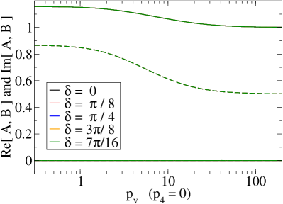
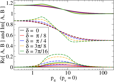
Figure 1: Real and imaginary parts of the inverse propagator functions $A$ (solid) and $B$ (dashed), at different angles $\delta$, obtained by un-Wick rotating the Euclidean solution as function of $p_{v}$ at $p_{4}=0$, corresponding to the spacelike $p^{2}$ axis (left) and as function of $p_{4}$ at $p_{v}=0$, along a line in the complex $p_{4}{\rm e}^{-i\,\delta}$ plane (right); $\delta=\pi/2$ would be the timelike axis. On the right we also show our results of rotating the magnitude of $p$ from the spacelike region towards the timelike region, which are indistinguishable at the scale shown. Parameters are $m_{0}=0.5$, $\mu=1.0$, $\Lambda=10.0$, and $\alpha=0.5$.

In Fig. 1 we present solutions of the DSE in the Feynman gauge obtained by un-Wick rotating $p_{4}$. When un-Wick rotating $p_{4}$ from Euclidean metric, we solve the DSE on a slice in the complex $p^{2}={\rm e}^{i\,2\delta}p_{4}^{2}+p_{v}^{2}$ plane; the boundaries of this slice are given by $(p_{4}=0,p_{v})$, which corresponds to the spacelike axis, and by $(p_{4},p_{v}=0)$, which approaches the timelike axis in the limit $\delta\to\pi/2$. The results for $A(p_{4}=0,p_{v})$ and $B(p_{4}=0,p_{v})$, i.e. on the spacelike axis, are indeed independent of the angle $\delta$, and purely real, as is shown in the left panel of Fig. 1. In the right panel, we show our results as function of $p_{4}$ for $p_{v}=0$, in wich case we do see a dependence on the angle $\delta$, as expected; furthermore, both $A$ and $B$ develop an imaginary part, which increases in magnitude with increasing $\delta$. However, as we approach $\delta=\pi/2$, the numerics becomes unstable due to singularities in the propagators, which prevents us from actually reaching the timelike axis.

3.2 Rotating the spacelike region to the timelike region

Alternatively, we can rotate the DSE from the Euclidean spacelike axis towards the timelike axis by applying the transformation

$$p\to{\rm e}^{-i\delta}\,p\,,\quad k\to{\rm e}^{-i\delta}\,k\,,\quad dk\to{\rm e}^{-i\delta}\,dk\,,$$ (22)

on the magnitude of the (Euclidean) four-vectors, while continuing to use 4-dimensional hyperspherical coordinates, as was done in e.g. Refs. [8, 9]. With this technique we keep $p$ and $k$ real (and positive), and we retain the 4-dimensional symmetry. As long as the contribution along the arc at $k=\infty$ vanishes (and with the explicit PV regularization it does), we can neglect the contribution along this arc, and keep only the integration over $k$ from $0$ to $\infty$.

In the limit of $\delta=\pi/2$ this transformation becomes

$$p^{2}_{\mathrm{E}}\to-p^{2}_{\mathrm{E}}=p^{2}\,,\quad k^{2}_{\mathrm{E}}\to-k^{2}_{\mathrm{E}}=k^{2}\,\quad k_{\mathrm{E}}^{3}\,dk_{\mathrm{E}}\to k_{\mathrm{E}}^{3}\,dk_{\mathrm{E}}=k^{3}\,dk\,,$$ (23)

and effectively this gives us a the DSEs on the pure timelike axis with $p^{2}\geq 0$

$$B(p^{2}) = m_{0}-\frac{2\,g^{2}}{(2\pi)^{3}}\int_{0}^{\infty}k^{3}\,dk\frac{4\,B(k^{2})}{k^{2}\,A^{2}(k^{2})-B^{2}(k^{2})}\;$$ (24)

$$\times\int_{0}^{\pi}\sin^{2}\theta\,d\theta\;\frac{\Lambda^{2}-\mu^{2}}{(q^{2}-\mu^{2})(q^{2}-\Lambda^{2})}\,,$$

$$A(p^{2}) = 1-\frac{2\,g^{2}}{(2\pi)^{3}}\int_{0}^{\infty}k^{3}\,dk\frac{A(k^{2})}{k^{2}\,A^{2}(k^{2})-B^{2}(k^{2})}\,$$ (25)

$$\times\int_{0}^{\pi}\sin^{2}\theta\,d\theta\,\frac{2\,k\cos\theta}{p}\,\frac{\Lambda^{2}-\mu^{2}}{(q^{2}-\mu^{2})(q^{2}-\Lambda^{2})}\,.$$

Note Eqs. (24) and (25) are for timelike momenta only, $p^{2}\geq 0$, $k^{2}\geq 0$, and $q^{2}=(p-k)^{2}\geq 0$ – they are different from the DSEs in Minkowski metric, Eqs. (5) and (6). (Again singularities under the integrals are specified by the $i\epsilon$ prescription.)

For any $0<\delta<\pi/2$, this method gives the DSE along a line from $0$ to $\infty$ in the upper complex $p^{2}$ plane, rather than on a slice of the upper complex momentum plane. Furthermore, it remains an integral equation in one variable, rather than in two variables as with the method described in the previous subsection. This method is therefore numerically easier to implement, and leads to better numerical precision.

In the right panel of Fig. 1, we also include our results obtained with this method. Not surprisingly, the results of the two methods are essentially indistinguishable, at least at the scale shown. However, the method of rotating the magnitude of $p$ is much more accurate (for a similar numerical effort) than the explicit un-Wick rotation of the fourth component, because when we un-Wick rotate the fourth component, we break the 4-dimensional symmetry by treating the fourth component and the 3-vector components differently. Furthermore, we solve the propagator functions $A$ and $B$ as functions of two independent real variables, $p_{4}$ and $p_{v}$, for a given angle $\delta$ (or equivalently, as function of one complex variable $p^{2}=p_{4}^{2}{\rm e}^{i\,2\delta}+p_{v}^{2}$), whereas if we rotate the magnitude of $p$ the functions $A$ and $B$ remain function of only one essentially real variable. In particular, as $\delta$ approaches $\pi/2$, in the case of the un-Wick rotation we solve the DSE in the entire upper $p^{2}$ plane, whereas if we rotate the magnitude of $p$, we solve the DSE along a line from $0$ to $\infty$ close to the timelike axis. Clearly, the latter approach is more efficient numerically.

4 Results for the self-energy in the timelike region

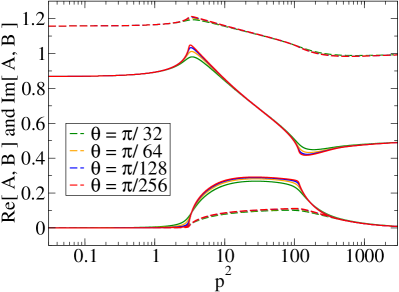
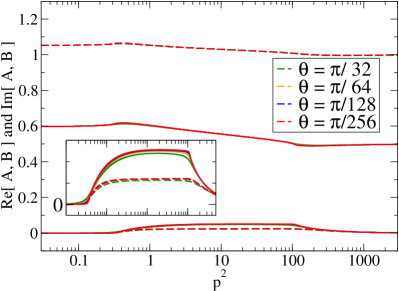
Figure 2: Real and imaginary parts of the inverse propagator functions $A$ (dashed) and $B$ (solid), at different angles $\theta$ close to the timelike axis. Both figures are with $m_{0}=0.5$ and PV mass $\Lambda=10$; and exchange mass $\mu=1.0$ and $\alpha=0.5$ (left) and massless vector boson and $\alpha=0.1$ (right).

In order to discuss our results as we approach the timelike region, it is more convenient to use $\theta=\pi/2-\delta$; with this notation the timelike axis corresponds to the limit $\theta\to 0$. For moderate values of the coupling (well below those corresponding to dynamical chiral symmetry breaking), we can achieve accurate results down to $\theta=\pi/256\approx 0.7^{\circ}$ by rotating the magnitude of $p$, whereas if we decrease $\theta$ below about $\theta=\pi/16\approx 11^{\circ}$, the un-Wick rotation becomes numerically challenging, requiring an effecient implementation on parallel high-performance computing systems.

In Fig. 2 we see that the imaginary parts of $A(p^{2})$ and $B(p^{2})$ become nonzero along the timelike axis. Furthermore, both the real parts and the imaginary parts of $A(p^{2})$ and $B(p^{2})$ develop kinks, that is, discontinuities in their derivatives. The location of these kinks is determined by the physical thresholds for the production of an exchange particle; these kinks occur at $(m_{\hbox{\scriptsize phys}}+\mu)^{2}$ and $(m_{\hbox{\scriptsize phys}}+\Lambda)^{2}$, where the pole mass $m_{\hbox{\scriptsize phys}}$ is determined from the zero of the inverse propagator, at $M(p^{2})=\sqrt{p^{2}}$.

These kinks are generally attributed to the integration over the propagator poles in Eqs. (5) and (6), where one (or more) denominator becomes zero. Mathematically, the kinks are caused by a pinch singularity due to the zeros of the exchange boson propagator and the fermion propagator in Eqs. (5) and (6).

4.1 Analytic structure and pole mass

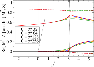
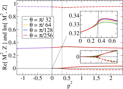
Figure 3: Real and imaginary parts of the dynamical mass squared, $M^{2}(p^{2})$ (solid), and wave function renormalization, $Z(p^{2})=1/A(p^{2})$ (dashed), in the spacelike and close to the timelike axis, again with $m_{0}=0.5$ and PV mass $\Lambda=10$. The extracted pole masses and residues are: $m=0.759$ and $Z(m^{2})=0.82$ for mass $\mu=1.0$ and $\alpha=0.5$ (left) and $m=0.58$ and $Z(m^{2})=0.34$ for massless vector boson and $\alpha=0.1$ (right).

In Fig. 3 we show our results for $M^{2}(p^{2})$ and $Z(p^{2})=1/A(p^{2})$ in the infrared region. The fermion propagator has a singularity at $p^{2}=M^{2}(p^{2})=m^{2}_{\hbox{\scriptsize phys}}$ in the timelike region. With a nonzero mass for the exchange boson, this singularity is a simple mass-pole (at least in Feynman gauge) – but neither the inverse propagator functions $A^{2}(p^{2})$ and $B(p^{2})$, nor the dynamical mass function $M(p^{2})$ shows any discontinuity or kink at this mass-pole.

The first kink or branch-point in the inverse propagator functions is located at $(m_{\hbox{\scriptsize phys}}+\mu)^{2}\geq m^{2}_{\hbox{\scriptsize phys}}$, as marked by the vertical dotted line in Fig. 3. At this kink, both the propagator itself and the inverse propagator functions have a branch-point, at which point the imaginary part becomes nonzero. With a nonzero exchange mass $\mu$, this kink occurs well beyond the mass-pole at $p^{2}=M^{2}(p^{2})$, and both the propagator and the inverse propagator functions are finite at this branch-point. However, in the limit of $\mu\to 0$, this branch-point coincides with the mass-pole singularity, as can be seen in the right panel of Fig. 3. Consequently, the propagator exhibits a more complicated singularity instead of a simple mass-pole, at which point the inverse propagator is zero, and a branch-cut starts along the timelike axis. The sign of the imaginary part is a consequence of the $i\epsilon$ prescription – or in the case of the un-Wick rotation, of the direction of the rotation.

Due to the PV regularization, the (inverse) propagator has a second kink along the timelike axis, located at $(m_{\hbox{\scriptsize phys}}+\Lambda)^{2}$, beyond which the imaginary parts fall off to zero, and the real parts of the (inverse) fermion propagator approach their bare (tree-level) values, see Fig. 2.

4.2 Spectral representation of the self-energy

With PB regularization, the integral representation for the scalar and vector self-energies can be written as

$$B(p^{2}) = m_{0}+\int_{0}^{\infty}ds\frac{\rho_{B}(s)}{p^{2}-s+i\varepsilon}\,\quad\text{with}\quad\rho_{B}(s)=-\text{Im}\left[B(s)/\pi\right]\,,$$ (26)

$$A(p^{2}) = 1+\int_{0}^{\infty}ds\frac{\rho_{A}(s)}{p^{2}-s+i\varepsilon}\,\quad\quad\text{with}\quad\rho_{A}(s)=-\text{Im}\left[A(s)/\pi\right]\,,$$ (27)

following the standard spectral representation of the propagators [25]. In principle, the spectral functions $\rho_{A,B}$ fully determine the scalar and vector self-energies, and thus the propagator.

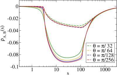
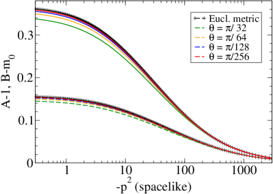
Figure 4: Left: Approximate spectral functions $\rho_{A,B}$ obtained at different angles $\theta$ close to the timelike axis for $m_{0}=0.5$, $\mu=1.0$, $\Lambda=10.0$, and $\alpha=0.5$. Right: Spacelike self-energies obtained from the approximate spectral functions, compared to the Euclidean solution.

In Fig. 4 we show on the left approximations to the spectral functions $\rho_{A,B}$ obtained from the imaginary parts of $A$ and $B$ at different angles $\theta$ close to the timelike axis. (Note that the angle $\theta$ is defined as the rotation angle for $p_{0}$ or the magnitude of $p$; in terms of the variable $s$ used in the spectral representation, this corresponds to an angle $2\theta$.) The right panel confirms that in the limit of $\theta\to 0$, these approximate spectral functions can indeed reproduce the Euclidean (spacelike) to high accuracy. With a more careful analysis and using a Mellin transformation, we can use these ‘approximate spectral representations’ at nonzero values of $\theta$ to calculate the self-energies in the entire slice of the upper complex $p^{2}$ plane, bounded by the real spacelike axis (negative $p^{2}$) and the line $p^{2}\,{\rm e}^{i\,2\theta}$. More details will be presented in Ref. [26].

5 Conclusion and outlook

This contribution presents a preliminary study of the nonperturbative fermion propagator in both the spacelike and near the timelike regions by investigating the fermion DSE in rainbow-ladder truncation in the Feynman gauge in a QED-like theory. Two methods to solve the Pauli–Villars regulated DSE were implemented to obtain the self-energies near the timelike axis, both relying on an analytic continuation of the Euclidean DSE into the complex momentum plane. In the first approach the energy component of the four-momenta are complex-rotated to bring the Euclidean formulation towards the Minkowski metric, while in the second method the magnitude of the four-vector $p$ is complex-rotated to rotate the spacelike axis towards the timelike axis. Both methods were used to compute the Dirac scalar and vector self-energies of the fermion near the timelike region. The second method showed to be much more accurate allowing calculations with angles as small as $\theta=\pi/256\approx 0.7^{\circ}$, quite close to the timelike axis. This is natural as with a fixed angle, in the first method the DSE has to be solved as function of two real variables, while in the second approach the scalar and vector self-energies depend on only one real variable, allowing a finer grid in this one variable.

The coupling constant was chosen sufficiently large for the solutions to allow for noticably nonperturbative effects, while below the value for dynamical chiral symmetry breaking. With a massive vector boson, the obtained nonperturbative fermion propagator has a mass-pole at $p^{2}=M^{2}(p^{2})=m^{2}_{\hbox{\scriptsize phys}}$ on the timelike axis, followed by a branch-cut starting at $p^{2}=(m_{\hbox{\scriptsize phys}}+\mu)^{2}$. With massless bosons, $\mu=0$, this branch-cut starts at the physical mass, and the mass-pole becomes a more complicated singularity. Finally, the imaginary part of the self-energies along the timelike axis were used to obtain the spectral densities, from which the spacelike self-energies were computed in good agreement with the Euclidean self-energies.

In the future, we intend to explore in more detail the analytic structure of the fermion propagator in the complex plane by, e.g., generalizing the spectral representation with finite $\theta$ associated with the study the solutions of Laplace equations using Mellin transform [26]; we also plan to extend these investigations to other gauges, in particular the Landau gauge, and to other theories. The next step will be to use these nonperturbative propagators in Minkowski metric for bound state calculations and to explore hadron structure directly in Minkowski space.

References

- [1] G. Eichmann, H. Sanchis-Alepuz, R. Williams, R. Alkofer and C. S. Fischer, Prog. Part. Nucl. Phys. 91, 1 (2016)
- [2] P. Maris and C. D. Roberts, Phys. Rev. C 56, 3369 (1997)
- [3] P. Maris and P. C. Tandy, Phys. Rev. C 60, 055214 (1999)
- [4] P. Maris and P. C. Tandy, Phys. Rev. C 62, 055204 (2000)
- [5] M. S. Bhagwat and P. Maris, Phys. Rev. C 77, 025203 (2008)
- [6] P. Maris, C. D. Roberts and P. C. Tandy, Phys. Lett. B 420, 267 (1998)
- [7] D. Atkinson and D. W. E. Blatt, Nucl. Phys. B 151, 342 (1979).
- [8] P. Maris, Nonperturbative analysis of the fermion propagator: Complex singularities and dynamical mass generation, Ph.D. thesis, U. of Groningen (1993)
- [9] P. Maris, Phys. Rev. D 50, 4189 (1994).
- [10] N. Nakanishi, Suppl. Prog. Theor. Phys. 43, 1 (1969)
- [11] V. Sauli, JHEP 0302, 001 (2003)
- [12] V. Sauli, Few Body Syst. 39, 45 (2006)
- [13] V. Sauli, J. Adam, Jr. and P. Bicudo, Phys. Rev. D 75, 087701 (2007)
- [14] S. Jia and M. R. Pennington, Phys. Rev. D 96, 036021 (2017)
- [15] K. Kusaka and A. G. Williams, Phys. Rev. D 51, 7026 (1995)
- [16] K. Kusaka, K. M. Simpson and A. G. Williams, Phys. Rev. D 56, 5071 (1997)
- [17] V. A. Karmanov and J. Carbonell, Eur. Phys. J. A 27, 1 (2006)
- [18] V. Sauli, Few Body Syst. 49, 223 (2010)
- [19] T. Frederico, G. Salmè and M. Viviani, Phys. Rev. D 85, 036009 (2012)
- [20] T. Frederico, G. Salmè and M. Viviani, Phys. Rev. D 89, 016010 (2014)
- [21] J. Carbonell and V. A. Karmanov, Eur. Phys. J. A 46, 387 (2010)
- [22] W. de Paula, T. Frederico, G. Salmè and M. Viviani, Phys. Rev. D 94, 071901 (2016)
- [23] W. de Paula, T. Frederico, G. Salmè, M. Viviani and R. Pimentel, Eur. Phys. J. C 77, 764 (2017)
- [24] A. Castro, E. Ydrefors, W. de Paula, T. Frederico, J. H. De Alvarenga Nogueira and P. Maris, arXiv:1901.04266 [hep-ph], to appear in the proceedings of XLI RTFNB, Maresias, Brazil, Sept. 2018
- [25] C. Itzykson and J.-B. Zuber, Quantum Field Theory, McGraw-Hill, New York, 1985.
- [26] P. Maris, S. Jia, D. C. Duarte, W. de Paula, E. Ydrefors, and T. Frederico, in preparation (2019).