Computing local intersection multiplicity of plane curves via blowup

Abstract.

We prove that intersection multiplicity of two plane curves defined by Fulton’s axioms is equivalent to the multiplicity computed using blowup. The algorithm based on the latter is presented and its complexity is estimated. We compute for polynomials over $\mathbb{Q}$ and its algebraic extensions.

1. Introduction

The classical result in algebraic geometry on plane curves, Bézout’s theorem, states that the number of intersections of two curves with no common component equals to the product of their degrees provided

• the curves are defined in projective plane,

• the intersections are computed over an algebraically closed field,

• each intersection point is counted with proper multiplicity.

The most obscure part is the computation of the multiplicity of the intersection in a particular point, which is generally a challenging task from both computational and interpretation point of view ([FOV99, BS17]), i.e. its intersection number.

During the development of the subject, several definitions of the intersection number for two curves in a given point were formulated. Nowadays, the definition by [Ful89] is probably the most known and accepted. We cite it in Section 2.3. The definition gives already an algorithm for computing the intersection number and it was implemented in Magma by [HS10]. Their algorithm lists all points of intersection of two algebraic curves, together with their multiplicities.

In [Wal04], the intersection number of two curves in a given point is described as the number of intersections that appear instead of the given one after we wiggle the curves a little bit. If one of the curves is a line (or more generally a rational curve), the intersection number can be easily computed: if $(\varphi(t),\psi(t))$ is a parametrization of one curve, we plug it into the polynomial $g$ defining the other curve and then the multiplicity of intersection in the point $(\varphi(t_{0}),\psi(t_{0}))$ is the multiplicity of the root $t_{0}$ in the equation $g(\varphi(t),\psi(t))=0$. In case none of the curves is rational, the parametrization of branches by Puiseux series can be used.

Alternatively, the intersection multiplicity of two curves can be computed using resultants ([Gib98, Wal78]). This is proven to be equivalent to the intersection number given by Fulton ([SWPD08]).

The geometric meaning of intersection multiplicity is expressed by relating it to the infinitely near points of the curve. For example, in a point in common for two curves, sharing a first order infinitely near point corresponds to sharing a tangent line and sharing also a second order infinitely near point corresponds to sharing an osculating circle. The connection between the intersection number and the shared infinitely near points is well studied in [Wal04] using Puiseux series or in [Zar38] using valuations.

The infinitely near points are looked for using birational morphism of the plane called blowup, which we briefly explain in Section 2.2. In the paper, we give a proof that the number computed by counting the shared infinitely near points with their multiplicities is the same as the intersection number defined by Fulton, and this is the main result of the paper:

Theorem 3.9. Let $f,g\in k[x,y]$ be non-constant polynomials and $P\in\mathbb{A}^{2}(k)$ be a point. Then

$$\mathcal{B}_{P}(f,g)=I_{P}(f,g),$$

where $\mathcal{B}_{P}(f,g)$ is the intersection number computed using infinitely near points at $P$ common for curves defined by $f$ and $g$, and $I_{P}(f,g)$ is the intersection number of the curves defined by Fulton.

So we can use the infinitely near points when computing the intersection number. When comparing with the algorithm by [HS10], the proposed algorithm computes the intersection multiplicity only in one point. But the tests show that in case the intersection multiplicity in the given point is high (i.e. the point is singular for one or both curves, or the curves share more geometric invariants in the point), or in case the curves themselves are of high degree, our algorithm turns out to be more effective. The performance of the algorithm is discussed at the end of the paper.

2. Preliminaries

2.1. Notation and terminology

The assertions in the paper are proven under the assumptions that the field $k$ is algebraically closed and its characteristic is 0.

In the paper, we work in the affine plane over the field $k$. A curve in $\mathbb{A}^{2}$ is defined by a single non-constant polynomial from $k[x,y]$. A curve defined by a polynomial $f$ is denoted $C_{f}$. The points on/of a curve $C_{f}$ are all roots of $f$ with coordinates in $k$. The set of all points of a curve $C_{f}$ we denote by $V(f)$. We will distinguish e.g. a curve defined by $2y-x^{2}$ and a curve defined by $(2y-x^{2})^{2}$, but we will not distinguish curves defined by $2y-x^{2}$ and $3x^{2}-6y$. So there is a bijection between plane curves defined over $k$ and proper principal ideals $(f)$ in $k[x,y]$.

Let $C_{f}$ be a plane curve and let $P=(p_{x},p_{y})\in\mathbb{A}^{2}$ be a point. We can write

$$f=a_{00}+a_{10}(x-p_{x})+a_{01}(x-p_{y})+a_{20}(x-p_{x})^{2}+a_{11}(x-p_{x})(x-p_{y})+a_{02}(x-p_{y})^{2}+\dots$$

as a polynomial in $x-p_{x}$, $y-p_{y}$ (the Taylor series of $f$ at $P$). Then the multiplicity of $C_{f}$ at $P$ is the degree of the lowest term with non-zero coefficients of the Taylor series of $f$ at $P$ with nonzero coefficient, we denote it by $m_{P}(C_{f})$ or $m_{P}(f)$. In case $P=(0,0)$, we may shorten the notation as $m(C_{f})$ or $m(f)$.

If $\varphi\colon\thinspace\mathbb{A}^{2}\to\mathbb{A}^{2}$ is an affine transform of the plane, then $f^{\varphi}$ denotes the polynomial $f\circ\varphi^{-1}$ i.e. $f^{\varphi}$ is a polynomial describing the transform of the curve $C_{f}$. In particular, the points of $C_{f^{\varphi}}$ are exactly the images of the points of $C_{f}$ under the transform $\varphi$:

$$\varphi(P)\in V(f^{\varphi})\quad\text{if and only if}\quad P\in V(f).$$

2.2. Blowup

Blowing up ([Sha13, Cut18]) is a powerful tool for resolving singularities of plane curves. However a curve can be blown up also in a regular point and we use it for computing the intersection multiplicity of the curves.

When blowing up the affine plane $\mathbb{A}^{2}$ in a point $P=(p_{1},p_{2})$, we construct a surface $X\subset\mathbb{A}^{2}\times\mathbb{P}^{1}$ given by $X=V((x-p_{1})t_{1}-(y-p_{2})t_{0})$, where $(x,y)$ are the coordinates in $\mathbb{A}^{2}$ and $(t_{0}\colon\thinspace t_{1})$ are the homogeneous coordinates in $\mathbb{P}^{1}$. The blowup of $\mathbb{A}^{2}$ is the surface $X$ together with the birational morphism

$$\pi\colon\thinspace X\to\mathbb{A}^{2},\quad(x,y;t_{0}\colon t_{1})\mapsto(x,y).$$

If $C_{f}$ is a curve in $\mathbb{A}^{2}$, its blowup is the preimage of $C_{f}$ under $\pi$, i.e. it is the curve on $X$ defined by the polynomial $\pi^{*}f=f\circ\pi$. The blowup of $C_{f}$ consists of the strict transform, which geometrically is the closure of $\pi^{-1}(V(f)\setminus\{P\})$ and algebraically it is the curve on $X$ defined by the saturation ideal $(\pi^{*}f):(x-p_{1},y-p_{2})^{\infty}$, and the exceptional line, which is the preimage of $P$. We denote the strict transform of $C_{f}$ by $C_{f}^{\prime}$. The points where the strict transform $C_{f}^{\prime}$ meets the exceptional line are the first order infinitely near points of the curve $C_{f}$ at the point $P$.

Let the curves $C_{f}$ and $C_{g}$ both pass through a point $P$ and let us consider their blowups. Each first order infinitely near point at $P$ shared by both curves corresponds to a tangent at $P$ that the curves $C_{f}$ and $C_{g}$ have in common.

When working with the strict transform of a curve $C_{f}$ contained in $X$, we pass to an affine chart of $X$ isomorphic to $\mathbb{A}^{2}$, for example the chart with $t_{0}\neq 0$. Then the strict transform $C_{f}^{\prime}$ is described by one polynomial and we will denote it $f^{\prime}$, so locally $C_{f}^{\prime}=C_{f^{\prime}}$.

Proposition 2.1.

Let $\varphi$ be an affine change of coordinates, which takes the curve $C_{f}$ to a curve $C_{g}$. Then $\varphi$ induces a linear map that takes the strict transform of $C_{f}$ after blowing up in $P\in V(f)$ to the strict transform of $C_{g}$ after blowing up in $\varphi(P)$.

Remark 2.2.

When blowing up a curve $C_{f}$ at $P$, by Proposition 2.1, we may assume $P=(0,0)$. Then we can write

(1) $$f=F+f_{1}$$

with $F$ being the form of degree $m(f)$ and $f_{1}$ containing the terms in $f$ of higher degree. The tangents of $C_{f}$ at $P=(0,0)$ correspond to the linear factors of $F$. The blowup of $C_{f}$ lays on the surface $X=V(xt_{1}-yt_{0})\subset\mathbb{A}^{2}\times\mathbb{P}^{1}$. By Proposition 2.1, we may also assume that the $y$-axis is not tangent to $C_{f}$ at $(0,0)$, so $x$ is not a factor of $F$ in (1). Then all first order infinitely near points of $C_{f}$ at $(0,0)$ are contained in the affine chart of $X$ with $t_{0}\neq 0$. Hence, the blowup of $C_{f}$ is locally described by

(2) $$f(x,xz)=x^{m(f)}(F(1,z)+xf_{2}(x,z))\quad\textrm{ for some }\quad f_{2}\in k[x,z],$$

where $z=t_{1}/t_{0}$. As usually done, we replace $z$ by $y$ in (2), so $x^{m(f)}$ corresponds to the exceptional line including its multiplicity $m(f)$ and

$$f^{\prime}(x,y)=F(1,y)+xf_{2}(x,y)$$

is a polynomial defining locally the strict transform $C_{f}^{\prime}$ with all exceptional points of $C_{f}$ at $(0,0)$ contained in the considered affine chart.

Let $C_{f}$ be a curve and $P\in V(f)$ be a point. After blowing up $C_{f}$ at $P$, we obtain $C_{f}^{\prime}$ containing the first order infinitely near points of $C_{f}$ at $P$. We can continue blowing up $C_{f}^{\prime}$ at such a point and obtain a transform of $C_{f}^{\prime}$ containing the first order infinitely near points of $C_{f}^{\prime}$ at the considered point, hence they are the second order infinitely near points of $C_{f}$ at $P$. Following the pattern, we define the infinitely near points of $C_{f}$ at $P$ of order $r$ for any $r\in\mathbb{N}^{+}=\mathbb{N}\setminus\{0\}$. In this way, we actually obtain a rooted tree of infinitely near points of $C_{f}$ at $P$. The root corresponds to the point $P$ and all other vertices correspond to infinitely near points of $C_{f}$ at $P$, where the direct descendants corresponds to all the different first order infinitely near points of the considered point. The tree is called the configuration of infinitely near points of $C_{f}$ at $P$. By the length of the configuration we refer to the number of consecutive blowups computed in order to find the configuration.

Proposition 2.3.

Let $C_{f},C_{g}$ be plane curves and let $P$ be a regular point of both $C_{f}$ and $C_{g}$. If for any $n\in\mathbb{N}^{+}$ the configurations of infinitely near points of length $n$ of $C_{f}$ and $C_{g}$ coincide, then $C_{f}$ and $C_{g}$ share a common component through $P$.

Proof.

[Lip94], Theorem 2.1. ∎

2.3. Local intersection number

We recall the basic knowledge and the definition of intersection of plane curves by [Ful89].

Theorem-Definition 2.4.

Let $C_{f},C_{g}$ be plane curves and let $P\in\mathbb{A}^{2}(k)$ be a point. There is a unique intersection number $I_{P}(f,g)$ defined for all plane curves $C_{f},C_{g}$ and all points $P\in\mathbb{A}^{2}(k)$ satisfying the following properties:

1. If $C_{f},C_{g}$ have no common component passing through $P$, then $I_{P}(f,g)$ is a non-negative integer; otherwise $I_{P}(f,g)=\infty$.

2. $I_{P}(f,g)=0$ if and only if $P\notin V(f)$ or $P\notin V(g)$.

3. If $\varphi$ is an affine change of coordinates, then $I_{P}(f,g)=I_{\varphi(P)}(f^{\varphi},g^{\varphi})$,

4. $I_{P}(f,g)=I_{P}(g,f)$.

5. $I_{P}(f,g)\geq m_{P}(f)m_{P}(g)$, where the equality occurs if and only if $C_{f}$ and $C_{g}$ have no common tangent line at $P$ (so called transversal intersection).

6. $I_{P}(f_{1}f_{2},g)=I_{P}(f_{1},g)+I_{P}(f_{2},g)$ for any $f_{1},f_{2}\in k[x,y]$.

7. $I_{P}(f,g)=I_{P}(f,g+hf)$ for any $h\in k[x,y]$.

3. Local properties of blowups of intersection.

Definition 3.1.

Let $C_{f},C_{g}$ be plane curves and let $P\in\mathbb{A}^{2}$ be a point. Let $C_{f}^{\prime},C_{g}^{\prime}$ be the strict transforms of $C_{f},C_{g}$ respectively under the blowing up the plane at the point $P$. Then, we define the number

$$\mathcal{B}_{P}(f,g)=\begin{cases}\infty,\quad\text{ if }C_{f}\text{ and }C_{g}\text{ share a component passing through }P,\\ 0,\quad\text{ if }P\notin V(f)\cap V(g),\\ m_{P}(f)m_{P}(g)+\sum_{Q}\mathcal{B}_{Q}(f^{\prime},g^{\prime})\quad\text{ otherwise},\end{cases}$$

where the sum in the last case runs through all the first order infinitely near points $Q$ common to $C_{f}$ and $C_{g}$. The number $\mathcal{B}_{P}(f,g)$ may sometimes be denoted also by $\mathcal{B}_{P}(C_{f},C_{g})$.

Lemma 3.2.

Let $C_{f},C_{g}$ be curves having no common component passing through $P$. Then the computation of $\mathcal{B}_{P}(f,g)$ according to Definition 3.1 terminates after finitely many steps. More precisely, there exist $r\in\mathbb{N}^{+}$ such that the curves $C_{f}$ and $C_{g}$ have no infinitely near point at $P$ of order $r$ in common.

Proof.

By blowing up $C_{f}$ and $C_{g}$ in $P$ and tracking the common infinitely near points at $P$, in each branch either the computation stops because there are no common infinitely near points, or after finitely many steps we arrive to the situation that we need to compute $\mathcal{B}_{P}(f,g)$, where $P$ is regular in both $C_{f}$ and $C_{g}$ ([Wal04]), Theorem 3.4.4.

So assume now that $P$ is regular in $C_{f}$ and $C_{g}$ and both curves share the common tangent at $P$. Assume that after blowing up at $P$ their strict transforms again share a tangent in the common infinitely near point, and that this situation reappears in each step. Then by Proposition 2.3 the components of $(f)$ and $(g)$ through $P$ coincide, a contradiction. ∎

Remark 3.3.

We use Lemma 3.2 in the proofs of the following propositions about $\mathcal{B}$ as follows: for given $P$, $C_{f}$ and $C_{g}$, we want to prove a claim about $\mathcal{B}_{P}(f,g)$. If $P\notin V(f)$ or $P\notin V(g)$ or $P\in V(f)\cap V(g)$ but $C_{f}$ and $C_{g}$ intersect transversally in $P$, we prove the claim about $\mathcal{B}$ directly (the start of the induction). In other cases we will prove it, provided the claim holds for $\mathcal{B}_{Q}(C_{f}^{\prime},C_{g}^{\prime})$, where $C_{f}^{\prime}$ and $C_{g}^{\prime}$ are the strict transforms of $C_{f}$ and $C_{g}$ after blowing up at $P$, and $Q$ is a common first order infinitely near point at $P$. So the induction step is to prove the claim for $\mathcal{B}_{P}(f,g)$ provided the claim is true for $\mathcal{B}_{Q}(\tilde{f},\tilde{g})$, where the configurations of the infinitely near points of $\tilde{f}$ resp. $\tilde{g}$ at $Q$ (see the commentary before Proposition 2.3) have smaller length than those of $f$ resp. $g$ at $P$. We refer to this proving style as the blowup induction.

In the rest of the section we will prove that the number $\mathcal{B}_{P}(f,g)$ computed recursively as in Definition 3.1 is exactly the intersection number $I_{P}(f,g)$. We do it by verifying that $\mathcal{B}_{P}(f,g)$ satisfies the properties in Definition 2.4.

Proposition 3.4.

If $\varphi$ is an affine change of coordinates, then

$$\mathcal{B}_{P}(f,g)=\mathcal{B}_{\varphi(P)}(f^{\varphi},g^{\varphi}).$$

Proof.

Affine change of coordinates taking $C_{f}$ to $C_{f^{\varphi}}$ and $C_{g}$ to $C_{g^{\varphi}}$ induces locally an affine change of coordinates taking $C_{f}^{\prime}$ to $C_{f^{\varphi}}^{\prime}$ and $C_{g}^{\prime}$ to $C_{g^{\varphi}}^{\prime}$ (Proposition 2.1). So the infinitely near points of $C_{f}$ are mapped to the infinitely near points of $C_{f^{\varphi}}$; the same holds for $C_{g}$ and $C_{g^{\varphi}}$.

Further, the affine change preserves the multiplicity of a curve in a point, so $m_{\varphi(P)}(f^{\varphi})=m_{P}(f)$. Hence the computation of $\mathcal{B}_{\varphi(P)}(f^{\varphi},g^{\varphi})$ is the same as the computation of $\mathcal{B}_{P}(f,g)$. ∎

Proposition 3.5.

Let $C_{f},C_{g}$ have no common component passing through $P$ and let $f=uv$. Then

$$\mathcal{B}_{P}(f,g)=\mathcal{B}_{P}(u,g)+\mathcal{B}_{P}(v,g).$$

Proof.

We note that the set of the first order infinitely near points of $C_{f}=C_{uv}$ at $P$ is the union of the sets of the first order infinitely near points of $C_{u}$ and $C_{v}$ at $P$. For, the first order infinitely near points depend only on the lowest degree form of the polynomial defining the curve, and the lowest degree form of $f$ is the product of those of $u$ and $v$.

We proceed by blowup induction, see Remark 3.3. First, let the curves $C_{f}$ and $C_{g}$ have no common first order infinitely near point at $P$. Then the pairs $C_{u},C_{g}$ and $C_{v},C_{g}$ also have no common infinitely near point at $P$. Therefore

$$\mathcal{B}_{P}(f,g)=m_{P}(f)m_{P}(g)=m_{P}(u)m_{P}(g)+m_{P}(v)m_{P}(g)=\mathcal{B}_{P}(u,g)+\mathcal{B}_{P}(v,g).$$

In a general case, we may assume $P=(0,0)$ and the $y$-axis in neither tangent to $C_{u}$, $C_{v}$ nor to $C_{g}$ at $P$, by Proposition 3.4. Then one checks easily (see Remark 2.2) that after blowing up $C_{f}$ in $P$ we have $(uv)^{\prime}=u^{\prime}v^{\prime}$ for the polynomials defining the strict transforms $C_{f}^{\prime}$. Again, since the first order infinitely near points of $C_{u}$ and $C_{v}$ are all among the first order infinitely near points of $C_{f}=C_{uv}$, it holds

(3) $$\mathcal{B}_{P}(f,g) = m_{P}(f)m_{P}(g)+\textstyle{\sum_{Q}\mathcal{B}_{Q}((uv)^{\prime},g^{\prime})}$$

$$= (m_{P}(u)+m_{P}(v))m_{P}(g)+\textstyle{\sum_{Q}\mathcal{B}_{Q}(u^{\prime}v^{\prime},g^{\prime})},$$

where the sum runs through the first order infinitely near points at $P$ that are shared by $C_{uv}$ and $C_{g}$. Now, we can continue by induction

$$(\ref{eq:5}) = m_{P}(u)m_{P}(g)+m_{P}(v)m_{P}(g)+\textstyle{\sum_{Q}\mathcal{B}_{Q}(u^{\prime},g^{\prime})}+\textstyle{\sum_{Q}\mathcal{B}_{Q}(v^{\prime},g^{\prime})}$$

$$= \mathcal{B}_{P}(u,g)+\mathcal{B}_{P}(v,g).$$

∎

We still need to verify the last property of $\mathcal{B}_{P}$. To do this, we first study a special kind of generators of an ideal $I$.

Definition 3.6.

Let $I=(f,g)\subset k[x,y]$ be an ideal. We say that $f,g$ is a max-order basis of $I$, if $m(f)\leq m(g)$ and for every $\tilde{g}\in I$ such that $(f,\tilde{g})=(f,g)$ we have that $m(\tilde{g})\leq m(g)$.

Example.

A max-order basis of the ideal is not unique: for example $x,y^{2}$ is a max-order basis of the ideal they generate, but also $x,y^{2}+x^{3}$ is a max-order basis of the same ideal. On the other hand, not every ideal has a max-order basis, for example

$$(x^{2}-x,xy)=(x^{2}-x,x^{2}y)=(x^{2}-x,x^{3}y)=\dots.$$

Lemma 3.7.

Let $C_{f},C_{g}$ be curves with no common component through $(0,0)$. Then $(f,g)$ has a max-order basis. Moreover, if $m(f)\leq m(g)$ then there exists $h\in k[x,y]$ such that $f,g+hf$ is a max-order basis.

Proof.

Consider the ideal $(f,g)$. By $F$ we denote the lowest degree form of $f$ and similarly let $G$ be the lowest degree form of $g$.

It holds that $f,g$ is a max-order basis of $(f,g)$ with $m(f)\leq m(g)$ if and only if the $G$ is not divisible by $F$.

So if $f,g$ is not a max-order basis of $(f,g)$, then $G$ factors as $G=FH$, $H$ being a form. We replace $g$ by $g+Hf$ and get a new basis of the ideal: $(f,g)=(f,g+Hf)$ with $m(g+Hf)>m(g)$. The process stops, for otherwise there would be a polynomial $\tilde{g}$ with $m(\tilde{g})>\deg(f)\deg(g)$ such that $(f,\tilde{g})=(f,g)$, which would be a contradiction to Bézout’s theorem. Hence, we arrive to $g+hf$ such that $(f,g+hf)=(f,g)$ and $f,g$ is a max-order basis, after finitely many steps . ∎

Proposition 3.8.

Let $C_{f},C_{g}$ have no common component passing through $P$. Then

$$\mathcal{B}_{P}(f,g+hf)=\mathcal{B}_{P}(f,g)$$

for any $h\in k[x,y]$.

Proof.

Again by Proposition 3.4, we assume $P=(0,0)$ and that the $y$-axis is not tangent to $C_{f}$ nor to $C_{g}$ at $P$. Hence, the strict transforms of curves constructed as described in Remark 2.2 contain all first order infinitely near points of $C_{f}$ a $C_{g}$. We proceed by the blowup induction, see Remark 3.3.

First, we solve the trivial cases.

1. Let $m(f)=m(g)=1$ with $C_{f}$ and $C_{g}$ intersecting transversally in $P=(0,0)$. Then the curves $C_{f}$ and $C_{g}$ have no infinitely near point in common. The same holds for $C_{f}$ and $C_{g+hf}$. To check it, one distinguishes two cases: if $m(h)>0$, then $g+hf$ has the same linear form as $g$, and if $m(h)=0$, the linear form of $g+hf$ is indeed different from the one of $g$ but again is no multiple of the one of $f$. So $\mathcal{B}_{P}(f,g+hf)=\mathcal{B}_{P}(f,g)=1$.

2. Let $m(f)=0$, $m(g)\geq 1$, then $\mathcal{B}_{P}(f,g)=\mathcal{B}_{P}(f,g+hf)=0$.

3. Let $m(f)\geq 1$, $m(g)=0$, then also $m(g+hf)=0$ and again $\mathcal{B}_{P}(f,g)=\mathcal{B}_{P}(f,g+hf)=0$.

Now, we use the hypothesis, that the assertion holds for $\mathcal{B}_{P}(f^{\prime},(g+hf)^{\prime})$, i.e. that

$$\mathcal{B}_{P}(f^{\prime},(g+hf)^{\prime}+\tilde{h}f^{\prime})=\mathcal{B}_{P}(f^{\prime},(g+hf)^{\prime})$$

for any $\tilde{h}\in k[x,y]$, and we prove it for $\mathcal{B}_{P}(f,g+hf)$ by case distinction.

Let $f=F+f_{1}$, where $F$ is the form consisting of lowest degree terms, so $\deg(F)=m(f)$, and $f_{1}$ is the polynomial containing the rest of $f$. Similarly, $g=G+g_{1}$ and $h=H+h_{1}$. For the polynomials locally defining the strict transforms, we have $f^{\prime}(x,y)=F(1,y)+xf_{2}(x,y)$ for some $f_{2}\in k[x,y]$, similarly for $g^{\prime}$ and $h^{\prime}$.

Case 1: Let $m(f)>m(g)$. An easy verification shows that

$$(g+hf)^{\prime}=g^{\prime}+x^{m(h)+m(f)-m(g)}h^{\prime}f^{\prime}.$$

Since the set of the first order infinitely near points of a curve at the point $P=(0,0)$ depends only on the form of the lowest degree, those of $C_{g+hf}$ are the same as those of $C_{g}$. So

$$\mathcal{B}_{P}(f,g+hf) = m(f)m(g+hf)+\textstyle{\sum_{Q}\mathcal{B}_{Q}(f^{\prime},(g+hf)^{\prime})}$$

$$= m(f)m(g)+\textstyle{\sum_{Q}\mathcal{B}_{Q}(f^{\prime},g^{\prime}+x^{m(h)+m(f)-m(g)}h^{\prime}f^{\prime})}$$

$$= m(f)m(g)+\textstyle{\sum_{Q}\mathcal{B}_{Q}(f^{\prime},g^{\prime})}$$

$$= \mathcal{B}_{P}(f,g),$$

where the sum runs through the first order infinitely near points of $C_{f}$ at $P$, and the third equality follows from the induction hypothesis.

Case 2: We assume that $f,g$ is a max-order basis of $(f,g)$ with $m(f)\leq m(g)$ and that $m(hf)\geq m(g)$, so $f,g+hf$ is also a max-order basis of $(f,g)$.

Again, we conclude that $C_{g}$ and $C_{g+hf}$ share the same first order infinitely near points at $P$ with $C_{f}$: it is straightforward, if $m(hf)>m(g)$, since in this case $C_{g}$ and $C_{g+hf}$ have the same first infinitely near points at $P$. A little more care is required if $m(hf)=m(g)$: here for sure $m(g+hf)=m(g)$ because $f,g$ is a max-order basis for $(f,g)$. Therefore, the form of degree $m(g)=m(f)+m(h)$ in $g+hf$ does not vanish and the $y$-coordinates of the infinitely near points of $g+hf$ are given by the equation $G(1,y)+H(1,y)F(1,y)=0$. From this we already easily check that the first order infinitely near points shared by $C_{f}$ and $C_{g+fh}$ are the same as the first order infinitely near points shared by $C_{f}$ and $C_{g}$.

For the polynomial defining the strict transform of $C_{g+hf}$ the direct computation shows that

$$(g+hf)^{\prime}=g^{\prime}+x^{m(f)+m(h)-m(g)}h^{\prime}f^{\prime}.$$

So we have exactly the same computation as in Case 1 showing that

$$\mathcal{B}_{P}(f,g+hf)=\mathcal{B}_{P}(f,g).$$

Case 3: We assume that $f,g$ is a max-order basis of $(f,g)$ with $m(f)\leq m(g)$ and that $m(hf)<m(g)$, so in this case $f,g+hf$ is not a max-order basis of $(f,g)$.

In this case, we have that

$$(g+hf)^{\prime}=x^{m(g)-m(f)-m(h)}g^{\prime}+h^{\prime}f^{\prime}$$

and the set of the first order infinitely near points of $C_{g+hf}$ at $P=(0,0)$ is the union of those of $C_{f}$ and those of $C_{h}$, so the following sum goes through the first order infinitely near points of $C_{f}$.

(4) $$\mathcal{B}_{P}(f,g+hf) = m(f)m(g+hf)+\textstyle{\sum_{Q}\mathcal{B}_{Q}(f^{\prime},(g+hf)^{\prime})}$$

$$= m(f)m(hf)+\textstyle{\sum_{Q}\mathcal{B}_{Q}(f^{\prime},x^{m(g)-m(f)-m(h)}g^{\prime}+h^{\prime}f^{\prime})}$$

$$= m(f)m(hf)+\textstyle{\sum_{Q}\mathcal{B}_{Q}(f^{\prime},x^{m(g)-m(f)-m(h)}g^{\prime})}$$

(5) $$= m(f)m(hf)+\textstyle{\sum_{Q}(m(g)-m(f)-m(h))\mathcal{B}_{Q}(f^{\prime},x)}+\textstyle{\sum_{Q}\mathcal{B}_{Q}(f^{\prime},g^{\prime})}$$

$$= m(f)m(hf)+(m(g)-m(f)-m(h))m(f)+\textstyle{\sum_{Q}\mathcal{B}_{Q}(f^{\prime},g^{\prime})}$$

$$= m(f)m(g)+\textstyle{\sum_{Q}\mathcal{B}_{Q}(f^{\prime},g^{\prime})}$$

(7) $$= \mathcal{B}_{p}(f,g).$$

Here (4) follows from the induction hypothesis, (5) follows from Proposition 3.5. The equality (3) follows from the fact that $C_{f}$ has exactly $m(f)$ counted with multiplicities infinitely near points at $P$ and none of them coinciding with those of $x$. Finally (7) follows from the fact that $\mathcal{B}_{Q}(f^{\prime},g^{\prime})=0$ if $Q$ does not belong to the first order infinitely near points of $C_{g}$.

Case 4: We assume that $m(f)\leq m(g)$ and neither $f,g$ nor $f,g+hf$ is a max-order basis of the ideal they generate.

By Lemma 3.7, there is $p\in k[x,y]$ such that $f,g+pf$ is a max-order basis and therefore by Case 3

$$\mathcal{B}_{P}(f,g)=\mathcal{B}_{P}(f,g+pf).$$

On the other hand $g+hf+(p-h)f=g+pf$, so again by Case 3

$$\mathcal{B}_{P}(f,g+hf)=\mathcal{B}_{P}(f,g+pf),$$

and we get

$$\mathcal{B}_{P}(f,g+hf)=\mathcal{B}_{P}(f,g).$$

∎

Theorem 3.9.

$$\mathcal{B}_{P}(f,g)=I_{P}(f,g).$$

Proof.

It is the consequence of the proven propositions and Theorem-Definition 2.4. Directly from the definition of $\mathcal{B}_{P}(f,g)$ follows, that the computed number satisfies the properties (1), (2), (4) and (5) of Theorem 2.4. The remaining properties were verified in Propositions 3.4, 3.5, and 3.8. ∎

4. The Algorithm for computing the local intersection multiplicity

We implemented our algorithm in Sage for curves given over $\mathbb{Q}$. During the computations, we need to factorize an univariate polynomial into linear factors. It might happen that the polynomial does not factor over the field we work in at the point, and so we make a suitable algebraic extension to make the factorization possible.

Function:	IntersectionMultiplicity
Input:	$f,g\in k[x,y]$ representing two curves at $\mathbb{A}^{2}(k)$,
Output:	intersection multiplicity of $f$ and $g$ in the point $(0,0)$.

1. // the intersection multiplicity is at least the product of the orders
   $m_{f}$ := the degree of the lowest term on $f$
   $m_{g}$ := the degree of the lowest term on $g$
   $I$ := $m_{f}.m_{g}$

2. // take affine charts of the blowups of $f$ and $g$ in $(0,0)$
   $f_{1}$ := $x^{-m_{f}}f(x,xy)$
   $g_{1}$ := $x^{-m_{g}}g(x,xy)$

3. // find all infinitely near points shared by both curves
   $roots:=$ roots of $gcd(f_{1}(0,y),g_{1}(0,y))$;
   (if needed, make an algebraic extension of the base field so that $gcd(f_{1}(0,y),g_{1}(0,y))$ splits into linear factors;)

4. // run the algorithm for all shared infinitely near points
   for $r\in roots$:
   $I:=I+$ IntersectionMultiplicity$(f_{1}(x,y+r),g_{1}(x,y+r))$
   endfor

5. // if the curves $f$ and $g$ are both tangent to $y$-axis at $(0,0)$
   if $x$ divides the lowest forms of both $f$ and $g$ then
   // take the other affine charts of the blowup
   $f_{1}$ := $y^{-m_{f}}f(xy,y)$
   $g_{1}$ := $y^{-m_{g}}g(xy,y)$
   $I:=I+$ IntersectionMultiplicity$(f_{1}(x,y),g_{1}(x,y))$
   end if;

6. return $I$.  

5. Examples

5.1. Circle and ellipse

Let $C_{f}$ be the ellipse given by

$$f=5x^{2}+6xy+5y^{2}-10y$$

and $C_{g}$ be the circle given by

$$g=x^{2}+(y-1)^{2}-1.$$

In the exposition and in the figures, we denote the polynomial describing the strict transform of $C_{f}$ resp. $C_{g}$ after the $i$-th blowup by $f_{i}$ resp. $g_{i}$. The restriction of the blowup morphism to an affine chart is denoted by $\pi$. The intersection multiplicity of $C_{f}$ and $C_{g}$ in $(0,0)$ is found after performing three consecutive blowups, see Figure 1.

Firstly, both curves are regular in $(0,0)$, so each has only one infinitely near point of the first order at $(0,0)$. We find them by computing the strict transforms of $f$ and $g$

$$f_{1} = 5x+6xy+5xy^{2}-10y,$$

$$g_{1} = x+xy^{2}-2y.$$

The infinitely near points are the intersections of the strict transform with $y$-axis. We see that both curves intersect the $y$-axis in the point $(0,0)$. Hence

$$I_{(0,0)}(f,g)=1.1+I_{(0,0)}(f_{1},g_{1}).$$

The point $(0,0)$ is again regular for both $f_{1}$ and $g_{1}$. After the second blowup, we have

$$f_{2} = 5+6xy+5x^{2}y^{2}-10y,$$

$$g_{2} = 1+x^{2}y^{2}-2y$$

and we see that they share the first order infinitely near point, $(0,1/2)$. So

$$I_{(0,0)}(f_{1},g_{1})=1.1+I_{(0,1/2)}(f_{2},g_{2}).$$

The point $(0,1/2)$ is regular for both $f_{2}$ and $g_{2}$ and the curves intersect transversally there. We detect this in the algorithm after blowing up the curves in the point (before doing so we shift the point $(0,1/2)$ to $(0,0)$) and checking that the strict transforms

$$f_{3} = 5x(xy+1/2)^{2}+6xy+3+5x(xy+1/2)^{2}-10y,$$

$$g_{3} = x(xy+1/2)^{2}-2y$$

have no common point on $y$-axis. Therefore

$$I_{(0,1/2)}(f_{2},g_{2})=1.1.$$

After summing up, the intersection multiplicity of $C_{f}$ and $C_{g}$ in $(0,0)$ is equal to 3.

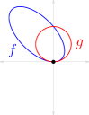
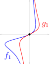
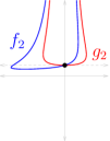
Figure 1. Computing intersection multiplicity of circle and ellipse in $(0,0)$.

5.2. Tacnode and ramphoid cusp

Let $C_{f}$ be the tacnode curve given by

$$f=2x^{4}-3x^{2}y+y^{2}-2y^{3}+y^{4}$$

and $C_{g}$ be the curve

$$g=(x/2)^{4}+(x/2)^{2}y^{2}-2(x/2)^{2}y-(x/2)y^{2}+y^{2}$$

(the ramphoid cusp). Again, after performing three consecutive blowups, the intersection multiplicity of the curves in $(0,0)$ is found, see Figure 2.

In this case, the point of intersection has multiplicity 2 for both curves. Both they have only one first order infinitely near point at $(0,0)$, namely $(0,0)$, therefore

$$I_{(0,0)}(f,g)=2.2+I_{(0,0)}(f_{1},g_{1}).$$

For curves $f_{1}$ and $g_{1}$, the point $(0,0)$ is again of multiplicity 2 in both cases. After blowing up in $(0,0)$ we see that the curve $f_{1}$ has at $(0,0)$ two first order infinitely near points: $(0,1)$ and $(0,2)$. Out of them only $(0,1)$ is shared with $g$, so

$$I_{(0,0)}(f_{1},g_{1})=2.2+I_{(0,1)}(f_{2},g_{2}).$$

Now the curves $f_{2}$ and $g_{2}$ are both regular at $(0,1)$ and they intersect transversally (i.e. share no infinitely near point), so

$$I_{(0,1)}(f_{2},g_{2})=1.1.$$

Summing up we see that $I_{(0,0)}(f,g)=9$.

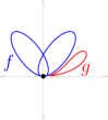
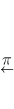
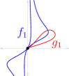
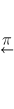
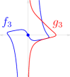
Figure 2. Computing intersection multiplicity of tacnode and ramphoid cusp in $(0,0)$.

5.3. Lemniscata of Bernoulli and the four-leaves-curve

Here, the lemniscata is given by

$$f=(x^{2}+y^{2})^{2}-(x^{2}-y^{2})$$

and the four-leaves-curve is given by

$$g=(x^{2}+y^{2})^{3}-(x^{2}-y^{2})^{2}.$$

In this case the computation of the intersection multiplicity of the two curves in $(0,0)$ proceeds

$$I_{(0,0)}(f,g) = 2.4+I_{(0,1)}(f_{1},g_{1})+I_{(0,-1)}(f_{1},g_{1})$$

$$= 8+1.2+1.2$$

$$= 12,$$

see Figure 3.

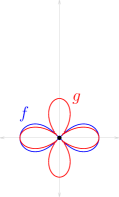
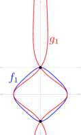
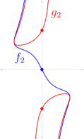
Figure 3. Computing intersection multiplicity of Bernoulli lemniscata and four-leaves-curve in $(0,0)$.

6. Performance

For comparison we implemented also the algorithm derived from axioms for the intersection number given by Fulton. When computing the intersection multiplicity of two curves in a given point using Fulton’s axioms of the intersection number, each step in the algorithm in relatively simple. The main operation there is finding new generators of the ideal $(f,g)$, $f,g\in k[x,y]$, which actually leads to a polynomial division with respect to the lexicographic ordering. The drawback of this approach is that the degrees of the polynomials are raising in each step. There are a lot of steps to be executed during the computation and there is actually no control of their number.

When computing the intersection multiplicity using blowup, we have to

• construct the strict transforms $f_{i+1}$ and $g_{i+1}$ of $f_{i}$ and $g_{i}$,

• find infinitely near points $Q_{j}$ shared by $f_{i+1}$ and $g_{i+1}$,

• move each $Q_{j}$ to $(0,0)$.

in each step. We know in advance that the $i$-th step deals with polynomials of degree $\mathcal{O}(i(\deg f+\deg g))$. We also have the upper bound for the number of steps, namely there are at most $\deg f\cdot\deg g$ steps executed during the computation. This is reflected in much better timing.

We implemented the algorithm in SageMath 8.3 ([The18]) and run it on processor x86_64, Intel(R) Core(TM) i3-3110M CPU @ 2.40GHz with memory 3.7 GiB.

In Table 1, the timings are given for both algorithms. They are obtained as the average of 10 randomly generated pairs of curves with a given degree and passing through $(0,0)$ with a given multiplicity. The intersection number is computed in $(0,0)$. The coefficients of the polynomials defining the curves are randomly generated integers from $-10$ to $10$.

	deg	m	$I(f,g)$	axioms	blowup	comment
1.	4	1	1	5.915 ms	1.452 ms	transversal intersection
2.	8	1	1	10.282 ms	1.823 ms	transversal intersection
3.	5	2	4	17.76 ms	1.169 ms	transversal intersection
4.	5	3	9	3407.24 ms	1.08 ms	transversal intersection
5.	6	3	9	–	1.412 ms	transversal intersection
6.	15	4	16	–	4.096 ms	transversal intersection
7.	5	3	10	346.75 ms	2.531 ms	a tangent in common
8.	5	3	11	113.39 ms	3.372 ms	a double tangent in common
9.	5	2	8	140.65 ms	8.107 ms	two tangents in common
10.	5	3	13,15	186.88 ms	6.113 ms	two tangents in common
11.	6	3	13	–	6.351 ms	two tangents in common
12.	15	3	13	–	24.05 ms	two tangents in common
13.	5	2	8	96.55 ms	33.23 ms	tangent cone $x^{2}+y^{2}$ in common

Table 1. “deg” – degree of the curves, “m” – multiplicity of $(0,0)$ on the curves, “$I(f,g)$” – the intersection multiplicity of the curves in $(0,0)$, “axioms” – time needed to compute the intersection multiplicity using the definition by Fulton, “blowup” – time needed to compute the intersection multiplicity via blowup, “–” – the algorithm did not finish in reasonable time

In some cases (indicated in the table) the algorithm using Fulton’s axioms for the intersection number did not finish. The last row in the table represents the situation where the extension of the field of rationals had to be constructed. Apparently this slowed the computation using blowup significantly (compare to the 9th row).

References

- [BS17] Eduard Boďa and Peter Schenzel. Local Bézout estimates and multiplicities of parameter and primary ideals. J. Algebra, 488:42–65, 2017.
- [Cut18] Steven Dale Cutkosky. Introduction to algebraic geometry, volume 188 of Graduate Studies in Mathematics. American Mathematical Society, Providence, RI, 2018.
- [FOV99] H. Flenner, L. O’Carroll, and W. Vogel. Joins and intersections. Springer Monographs in Mathematics. Springer-Verlag, Berlin, 1999.
- [Ful89] William Fulton. Algebraic curves. Advanced Book Classics. Addison-Wesley Publishing Company, Advanced Book Program, Redwood City, CA, 1989. An introduction to algebraic geometry, Notes written with the collaboration of Richard Weiss, Reprint of 1969 original.
- [Gib98] C. G. Gibson. Elementary geometry of algebraic curves: an undergraduate introduction. Cambridge University Press, Cambridge, 1998.
- [HS10] Jan Hilmar and Chris Smyth. Euclid meets Bézout: intersecting algebraic plane curves with the Euclidean algorithm. Amer. Math. Monthly, 117(3):250–260, 2010.
- [Lip94] Joseph Lipman. Proximity inequalities for complete ideals in two-dimensional regular local rings. In Commutative algebra: syzygies, multiplicities, and birational algebra (South Hadley, MA, 1992), volume 159 of Contemp. Math., pages 293–306. Amer. Math. Soc., Providence, RI, 1994.
- [Sha13] Igor R. Shafarevich. Basic algebraic geometry. 2. Springer, Heidelberg, third edition, 2013. Schemes and complex manifolds, Translated from the 2007 third Russian edition by Miles Reid.
- [SWPD08] J. Rafael Sendra, Franz Winkler, and Sonia Pérez-Díaz. Rational algebraic curves, volume 22 of Algorithms and Computation in Mathematics. Springer, Berlin, 2008. A computer algebra approach.
- [The18] The Sage Developers. SageMath, the Sage Mathematics Software System (Version 8.3), 2018. https://www.sagemath.org.
- [Wal78] Robert J. Walker. Algebraic curves. Springer-Verlag, New York-Heidelberg, 1978. Reprint of the 1950 edition.
- [Wal04] C. T. C. Wall. Singular points of plane curves, volume 63 of London Mathematical Society Student Texts. Cambridge University Press, Cambridge, 2004.
- [Zar38] Oscar Zariski. Polynomial Ideals Defined by Infinitely Near Base Points. Amer. J. Math., 60(1):151–204, 1938.