User-specified random sampling of quantum channels and its applications

Abstract

Random samples of quantum channels have many applications in quantum information processing tasks. Due to the Choi–Jamiołkowski isomorphism, there is a well-known correspondence between channels and states, and one can imagine adapting state sampling methods to sample quantum channels. Here, we discuss such an adaptation, using the Hamiltonian Monte Carlo method, a well-known classical method capable of producing high-quality samples from arbitrary, user-specified distributions. Its implementation requires an exact parameterization of the space of quantum channels, with no superfluous parameters and no constraints. We construct such a parameterization, and demonstrate its use in three common channel sampling applications.
Keywords: quantum tomography, quantum channels, quantum parameter estimation, Choi-Jamiołkowski isomorphism, error regions, plausible region, random sampling, Monte Carlo methods

I Introduction

Quantum channels, or completely positive (CP) and trace-preserving (TP) maps, are a central concept in describing the dynamics of quantum systems. They form the basic models for imperfect quantum operations used for quantum information processing (QIP). Random—according to some specified distribution—samples of quantum channels are needed in many QIP tasks, including the evaluation of the distributional average of channel-related quantities, the computation of error bars for quantum process tomography, the exploration of typical properties of quantum channels, the numerical optimization of functions of channels over a complicated landscape, and others.

Sampling from specific distributions over the quantum state space is a well-studied problem, with many different approaches, including the Monte Carlo (MC) technique for arbitrary distributions, and other methods for sampling from specific distributions Shang+1:15 ; Seah+1:15 ; Zyczkowski98 ; Zyczkowski99 ; Zyczkowski01 ; Blume10 ; Huszar12 ; YS19 . Due to the Choi–Jamiołkowski isomorphism Choi ; Jamiolkowski , which gives a correspondence between CP channels and states, these state sampling methods can be adapted to sample quantum channels. Indeed, in the recent work by Thinh et al. Thinh18 , a Metropolis–Hasting Markov chain (MHMC) MC approach was used to sample channels from arbitrary distributions, by sampling the purification of the Choi–Jamiołkowski state corresponding to the channel. References Geometry and Bruzda09 discuss a procedure for generating samples of quantum channels with a specific distribution on the channel space by making use of the channel-state correspondence. An alternative way of generating the same distribution of channels is to couple the input state and an ancilla initially in an arbitrary pure state by a Haar-random unitary operator and then taking the partial trace over the ancilla. See Ref. Bruzda10 for more discussion on the properties of the distribution of channels generated by these two procedures.

As a general method for sampling from arbitrary distributions, MC methods stand out in their wide-ranging applicability and efficiency. The MHMC variety of MC methods used, for example, in Ref. Thinh18 , however, suffer from strong correlations between sample points, and one requires large samples for reliable answers not biased by these correlations. This was observed, for instance, in the MHMC state sampling algorithm of Ref. Shang+1:15 . A significant improvement in the quality of the samples was seen when we switched to the Hamiltonian Monte Carlo (HMC) approach Seah+1:15 , reaffirming the advantage of HMC over MHMC MC also observed in other settings Neal96 ; Hajian07 ; Porter14 ; Neal11 ; Duane87 .

The HMC method requires the availability of a parameterization of the domain space with exactly the right number of parameters, with no superfluous parameters and no constraints. The parameterization of the channel/state space used in Ref. Thinh18 , which has superfluous parameters, cannot be used for HMC. The exact parameterization of states used in the HMC algorithm in Ref. Seah+1:15 gives, through the Choi–Jamiołkowski isomorphism, a parameterization of the set of all CP, but not necessarily TP, maps. The TP property has to be imposed as an explicit constraint, thus rendering the parameterization unsuitable in a HMC algorithm for sampling CPTP channels.

In this work, we construct one exact parameterization of the space of CPTP maps, with no superfluous parameters, and no constraints. This can then be used in a HMC procedure for sampling from arbitrary, user-specified, distributions over the channel space. To illustrate the usefulness of our parameterization and the HMC algorithm, we apply our methods to three quantum sampling problems. Our examples are focused on problems in quantum process tomography, reflecting the interests of the authors; our parameterization and the HMC method, however, are just as useful for sampling problems in other areas of QIP. As an aside, our construction exactly parameterizes the space of all bipartite mixed quantum states with the completely mixed state for one of the parties.

Here is the brief outline of our paper. We first review the Choi–Jamiołkowski isomorphism in Sec. II. Section III explains our main contribution: the exact parameterization of the space of CPTP channels. In Sec. IV, we illustrate the use of our parameterization in a HMC sampling algorithm through three examples from quantum process tomography: (a) the construction of error regions in process estimation; (b) marginal likelihood for estimating specific properties of the channel; (c) model selection among candidate channel families. The reader is referred to Ref. Seah+1:15 or Appendix A for an introduction to the HMC algorithm used here. We conclude in Sec. V.

II The channel-state duality

There are many ways of writing the CPTP map of a quantum channel. Given our desire to make the connection with the sampling of quantum states, we make use of the channel-state duality and describe the quantum channel by a state via the Choi–Jamiołkowski isomorphism. Here, we remind the reader of this isomorphism, and, in the process, define the notation used throughout the article.

We begin with the $d$-dimensional Hilbert space $\mathcal{H}$ describing the state vectors (pure states) of the system. We define a map $*:\mathcal{H}\rightarrow\mathcal{H}$,

$$*(|\psi\rangle)\equiv|\overline{\psi}\rangle\in\mathcal{H},\quad\textrm{for }|\psi\rangle\in\mathcal{H},$$ (1)

such that

$$\langle\overline{\psi}|\overline{\phi}\rangle=\langle\phi|\psi\rangle,\quad\forall|\psi\rangle,|\phi\rangle\in\mathcal{H},$$ (2)

and $*$ is “$*$-linear”, i.e.,

$$*\Bigl{(}\sum_{i}c_{i}|\psi_{i}\rangle\Bigr{)}=\sum_{i}c_{i}^{*}|\overline{\psi}_{i}\rangle,$$ (3)

where $c_{i}^{*}$ is the complex conjugate of $c_{i}$. Note that Eq. (2) specifies the $*$ map only up to a unitary transformation of no consequence. One specific realisation of the $*$ map, and what we use in our numerical examples below, is to first pick a basis $\{|i\rangle\}$ on $\mathcal{H}$, define $|\overline{i}\rangle\equiv|i\rangle$, and then extend the action of $*$ to arbitrary vectors using the $*$-linearity property. See also Sec. 3.1 in Ref. MUB10 for qubit examples of the $*$ map.

We extend the action of the $*$ map to adjoint vectors, $*(\langle\psi|)=\langle\overline{\psi}|=(|\overline{\psi}\rangle)^{\dagger}=[*(|\psi\rangle)]^{\dagger}$, and further to the set of operators on $\mathcal{H}$, denoted as $\mathcal{B}(\mathcal{H})$,

$$*\Bigl{(}\sum_{ij}c_{ij}|\psi_{i}\rangle\langle\phi_{j}|\Bigr{)}\equiv\sum_{ij}c_{ij}^{*}|\overline{\psi}_{i}\rangle\langle\overline{\phi}_{j}|.$$ (4)

We write $*(X)\equiv\overline{X}$, for any $X\in\mathcal{B}(\mathcal{H})$. Note that $\overline{X^{\dagger}}=(\overline{X})^{\dagger}$, and we denote $X^{\mathcal{T}}\equiv\overline{X}^{\dagger}$, a basis-independent transpose operation. If $X$ is non-negative, then so is $X^{\mathcal{T}}$.

Using the $*$ map, we define the vectorization map, a linear map from operators to vectors in a vector space $\mathcal{V}$, $\textrm{vec}:\mathcal{B}(\mathcal{H})\rightarrow\mathcal{V}$,

$$\textrm{vec}(|\psi\rangle\langle\phi|)\equiv*(|\phi\rangle)\otimes|\psi\rangle=|\overline{\phi}\rangle\otimes|\psi\rangle=|\overline{\phi}\,\psi\rangle,$$ (5)

for any $|\psi\rangle,|\phi\rangle\in\mathcal{H}$ and extended to all operators by linearity. We write, for any $X\in\mathcal{B}(H)$, $\textrm{vec}(X)\equiv|X\rangle\!\rangle\in\mathcal{V}$. Note the useful identity,

$$\textrm{vec}(ABC)=(C^{\mathcal{T}}\otimes A)\,\textrm{vec}(B).$$ (6)

Also, if $\{|i\rangle\}$ is an orthonormal basis for $\mathcal{H}$, then so is $\{|\overline{i}\rangle\}$. Consequently, the vectorized identity operator, $|\mathbbm{1}\rangle\!\rangle=\textrm{vec}(\mathbbm{1})=\sum_{i=1}^{d}|\overline{i}i\rangle$, can be regarded as a bipartite maximally entangled (unnormalized) state on $\mathcal{H}\otimes\mathcal{H}$.

Now, we are ready to state the channel-state duality. Consider a CP map, $\mathcal{E}:\mathcal{B}(\mathcal{H})\rightarrow\mathcal{B}(\mathcal{H})$, acting as $\mathcal{E}(\cdot)=\sum_{a}E_{a}(\cdot)E_{a}^{\dagger}$ for a (nonunique) set of Kraus operators $\{E_{a}\}$. We define

$$\rho_{\mathcal{E}} \equiv\sum_{a}|E_{a}\rangle\!\rangle\langle\!\langle E_{a}|=\sum_{a}(\mathbbm{1}\otimes E_{a})|\mathbbm{1}\rangle\!\rangle\langle\!\langle\mathbbm{1}|(\mathbbm{1}\otimes E_{a}^{\dagger})$$

$$=(\mathbbm{1}\otimes\mathcal{E}){\left(|\mathbbm{1}\rangle\!\rangle\langle\!\langle\mathbbm{1}|\right)},$$ (7)

where we have used the identity in Eq. (6); the $\mathbbm{1}$ in $\mathbbm{1}\otimes\mathcal{E}$ denotes the identity map. Thus defined, $\rho_{\mathcal{E}}$ is a nonnegative operator on $\mathcal{V}$; it can also be regarded as an unnormalized state (density operator) on the bipartite Hilbert space $\mathcal{H}\otimes\mathcal{H}\equiv\mathcal{H}_{1}\otimes\mathcal{H}_{2}$, labelling the two subsystems by $1$ and $2$. In the latter picture, one regards $|\mathbbm{1}\rangle\!\rangle\langle\!\langle\mathbbm{1}|$ as the density operator for a maximally entangled state on $\mathcal{H}\otimes\mathcal{H}$, and $\rho_{\mathcal{E}}$ is the density operator that results from the action of the map $\mathbbm{1}\otimes\mathcal{E}$ on it.

That $\rho_{\mathcal{E}}$ is invariant under a change of Kraus representation for the $\mathcal{E}$ is manifest in the last line of Eq. (II). We can turn the logic around: Any bipartite state on $\mathcal{H}\otimes\mathcal{H}$ possesses a spectral decomposition into eigenvectors, and the identification of those eigenvectors, with their corresponding (square root of the) eigenvalues, as vectorized Kraus operators immediately gives an associated CP map on $\mathcal{B}(\mathcal{H})$. Equation (II) hence states a duality between CP maps $\mathcal{E}$ and states $\rho_{\mathcal{E}}\geq 0$. $\rho_{\mathcal{E}}$ is sometimes called the “Choi state” of the CP map $\mathcal{E}$. Observe that

$$\mathcal{E}(X)=\textrm{tr}_{1}\{\rho_{\mathcal{E}}(X^{\mathcal{T}}\otimes\mathbbm{1})\}.$$ (8)

We are primarily interested in CP maps that are also TP. In this case, the state $\rho_{\mathcal{E}}$ dual to the CP and TP channel satisfies the partial trace condition,

$$\textrm{tr}_{2}(\rho_{\mathcal{E}})=\mathbbm{1},$$ (9)

i.e., $\mathcal{E}$ is CPTP if and only if $\rho_{\mathcal{E}}\geq 0$ and $\textrm{tr}_{2}(\rho_{\mathcal{E}})=\mathbbm{1}$. A simple count verifies that we have just the right number of parameters: A CP $\mathcal{E}$ is represented by $d^{4}$ real parameters—a positivity-preserving map that specifies how a $d^{2}$-element basis of operators on $\mathcal{H}$ is mapped back to itself—and this is the same number of real parameters needed to specify an unnormalized non-negative $\rho_{\mathcal{E}}$; the TP condition removes $d^{2}$ parameters, leaving $d^{2}(d^{2}-1)$ real parameters for a CPTP map, i.e., a quantum channel. Note that the set of $\rho_{\mathcal{E}}$s corresponding to quantum channels form a convex set of states, each with trace $d$. We denote the convex set of all $\rho_{\mathcal{E}}$ that satisfy Eq. (9) by $\mathscr{S}_{\mathrm{TP}}$, and refer to $\rho_{\mathcal{E}}\in\mathscr{S}_{\mathrm{TP}}$ as a TP state.

This duality between quantum channels and states enables us to sample quantum channels with algorithms for sampling quantum states (see the next section). Furthermore, the problem of process tomography—the estimation of the full description of a quantum channel acting on a quantum system—can be re-cast as that of state tomography. As the applications of our channel sampling algorithm discussed below are related to estimating quantum channels, we use the remainder of this section to recall this connection between state and process tomography, stemming from the channel-state duality MLEreview .

Quantum process tomography seeks to discover the full description of some unknown quantum channel $\mathcal{E}$, through $N$ uses of the channel. Standard strategies involve choosing a set of input states $\{\rho^{(i)}\}$, sending $N^{(i)}$ copies of state $\rho^{(i)}$ through the channel $\mathcal{E}$, and then measuring the output state using a POVM $\Pi^{(i)}\equiv\{\Pi_{k}^{(i)}\}$. For each $i$, the tomographic outcome probabilities come from the Born rule,

$$p_{k}^{(i)}=\textrm{tr}\{\Pi_{k}^{(i)}\mathcal{E}(\rho^{(i)})\}=\textrm{tr}\Bigl{\{}\rho_{\mathcal{E}}\Lambda_{k}^{(i)}\Bigr{\}},$$ (10)

where $\Lambda_{k}^{(i)}\equiv(\rho^{(i)})^{\mathcal{T}}\otimes\Pi_{k}^{(i)}$. Written in this manner, the expression for $p_{k}^{(i)}$ reminds one of the situation of state tomography of $\rho_{\mathcal{E}}$, where the set $\{\Lambda_{k}^{(i)}\}$ forms a pseudo-POVM in that $\Lambda_{k}^{(i)}\geq 0\ \forall k,i$, and $\sum_{k}\Lambda_{k}^{(i)}=\rho^{(i)}\otimes\mathbbm{1}$ for any $i$. Note that $\sum_{k}p_{k}^{(i)}=1$, as guaranteed by the TP condition in Eq. (9) together with the normalization $\textrm{tr}(\rho^{(i)})=1$.

The likelihood function for the data $D=\{D^{(i)}=(n_{1}^{(i)},n_{2}^{(i)},\ldots)\}$—$n_{k}^{(i)}$ denotes the number of clicks in detector $\Pi_{k}^{(i)}$ when $\rho^{(i)}$ is sent, and ${\sum_{k}n_{k}^{(i)}=N^{(i)}}$—collected is

$$L(D|\rho_{\mathcal{E}})=\prod_{i}L(D^{(i)}|\rho_{\mathcal{E}})=\prod_{i}{\left[\prod_{k}(p_{k}^{(i)})^{n_{k}^{(i)}}\right]},$$ (11)

where we omit the combinatorial factors that are needed for proper normalization but are not important here. Disregarding quantum constraints, the likelihood is maximized, over all $\{p_{k}^{(i)}\}$, by setting ${p_{k}^{(i)}=\frac{\mbox{\footnotesize$n_{k}^{(i)}$}}{\mbox{\footnotesize$N^{(i)}$}}}$; with quantum constraints, a constrained maximization of $L(D|\rho_{\mathcal{E}})$ over all permissible probabilities—those $p^{(i)}_{k}$s that could have come from a nonnegative $\rho_{\mathcal{E}}$ and which satisfy ${\sum_{k}p_{k}^{(i)}=1\ \forall i}$—yields what is known as the maximum-likelihood estimator (MLE) for $\rho_{\mathcal{E}}$ MLEreview .

III Parameterizing channels

III.1 Arbitrary channels

To obtain a sample of quantum channels according to some specified distribution, we generate Choi states $\rho_{\mathcal{E}}$ with the HMC algorithm. The HMC method demands a parameterization of the state space (in this case the space of $\rho_{\mathcal{E}}$) with no superfluous parameters and no external constraints. In Ref. Seah+1:15 , the ability to sample quantum states with the HMC algorithm was demonstrated using a parameterization of the full quantum state space. Because of the TP condition, sampling of quantum channels demands a parameterization of, not the full quantum state space as in Ref. Seah+1:15 , but only of the set $\mathscr{S}_{\mathrm{TP}}$ of TP states. Here, as our central result, we explain how to accomplish this.

We first choose a product basis $\{|\overline{i}j\rangle\}_{i,j=1}^{d}$ on $\mathcal{H}\otimes\mathcal{H}$ and represent $\rho_{\mathcal{E}}$ as a $d^{2}\times d^{2}$ matrix—also denoted as $\rho_{\mathcal{E}}$, to simplify notation—with complex entries. Positivity of $\rho_{\mathcal{E}}$ means that we can write $\rho_{\mathcal{E}}=A^{\dagger}A$, where $A$ is a $d^{2}\times d^{2}$ upper triangular complex matrix with real entries in the last column. The $d^{2}$ columns of $A$ are labelled using a double index,

$$A=\begin{pmatrix}|&|&&|\\ \varphi_{11}&\varphi_{12}&\dots&\varphi_{dd}\\ |&|&&|\end{pmatrix},$$ (12)

so that $\rho_{\mathcal{E}}=\sum_{ijkl=1}^{d}\varphi_{ij}^{\dagger}\varphi_{kl}|\overline{i}j\rangle\langle\overline{k}l|$, as the abstract, basis-independent object. Stacking the columns of $A$ to form columns with $d^{3}$ entries,

$$\varphi_{i}\equiv\begin{pmatrix}\varphi_{i1}\\ \varphi_{i2}\\ \vdots\\ \varphi_{id}\end{pmatrix},\quad\textrm{for }i=1,2,\ldots,d,$$ (13)

permits writing the TP condition in Eq. (9), that is ${\textrm{tr}_{2}(\rho_{\mathcal{E}})=\sum_{ij}{\left(\sum_{k}\varphi_{ik}^{\dagger}\varphi_{jk}\right)}|\overline{i}\rangle\langle\overline{j}|=\mathbbm{1}=\sum_{ij}\delta_{ij}|\overline{i}\rangle\langle\overline{j}|}$, as an orthonormality condition on the $\varphi_{i}$s,

$$\varphi_{i}^{\dagger}\varphi_{j}=\delta_{ij}\quad\textrm{for }i,j=1,2,\ldots,d.$$ (14)

Hence, to sample quantum channels, we simply need to find a parameterization for the orthonormal set $\{\varphi_{i}\}_{i=1}^{d}$.

Let us count the number of parameters needed. Since $A$ is upper triangular, $\varphi_{ik}$ has $(ik)+1$ generically nonzero entries, where $(ik)\equiv(i-1)d+(k-1)$ is a $d$-nary number. Each $\varphi_{i}$ thus has $K_{i}\equiv\sum_{k}[(ik)+1]=id^{2}-\frac{1}{2}d(d-1)$ nonzero entries. These nonzero entries are all complex, except for the $d^{2}$ of them in $\varphi_{dd}$, which are real. The orthonormality conditions on the $\varphi_{i}$s remove $d^{2}$ real parameters. Altogether then, the $\varphi_{i}$s are described by $2\sum_{i}K_{i}-d^{2}-d^{2}=d^{2}(d^{2}-1)$ real parameters, exactly the number needed to describe a quantum channel.

To specify an appropriate parametrization of the $\varphi_{i}$ set, it is convenient to reshuffle the rows of $\varphi_{i}$ so that all the identically-zero entries of each $\varphi_{i}$ are collected together. We first define the matrix

$$\Phi\equiv\begin{pmatrix}|&|&&|\\ \varphi_{1}&\varphi_{2}&\dots&\varphi_{d}\\ |&|&&|\end{pmatrix}.$$ (15)

Observe that the orthonormality conditions on the $\varphi_{i}$s translate into the requirement that $\Phi^{\dagger}\Phi=\mathbbm{1}$. Let $P$ be a $d^{3}\times d^{3}$ permutation matrix such that

$$\Psi\equiv P\Phi=\begin{pmatrix}|&|&&|\\ \psi_{1}&\psi_{2}&\dots&\psi_{d}\\ |&|&&|\end{pmatrix}$$ (16)

has columns $\psi_{i}$s, each of which is a reshuffled $\varphi_{i}$ with all identically zero entries located below the generically nonzero ones, i.e., the $k$th entry of $\psi_{i}$, which we denote as $\psi_{ik}$, is generally nonzero for $k=1,\ldots,K_{i}$, and zero for $k=K_{i}+1,\ldots,d^{3}$. Such a $P$ matrix exists because $A$ is upper triangular. Requiring $\Phi^{\dagger}\Phi=\mathbbm{1}$ is equivalent to demanding $\Psi^{\dagger}\Psi=\Phi^{\dagger}P^{-1}P\Phi=\mathbbm{1}$.

We are now ready to state the parameterization for the $\psi_{i}$s, thereby giving a parameterization for $\mathscr{S}_{\mathrm{TP}}$. We begin with $\psi_{d}$, parameterizing it with spherical coordinates so that it is normalized,

$$\psi_{dk}\equiv{\left\{\begin{array}[]{ll}\textrm{e}^{\textrm{i}\phi_{k}}(\cos\theta_{k-1})S_{k}&\textrm{for }k=1,\ldots,K_{d}\\ 0&\textrm{for }k=K_{d}+1,\ldots,d^{3}\end{array}\right.},$$ (19)

where $\theta_{0}\equiv 0$ fixed, and the $S_{k}$s are recursively defined as $S_{k}=(\sin\theta_{k})S_{k+1}$, with $S_{K_{d}}=1$. Here, the $\phi_{k}$s for the $\psi_{dk}$s that come from the real entries of $\varphi_{dd}$ are understood to be set to zero (which ones they are, depends on the choice of $P$). $\psi_{d}$ is hence parameterized by real parameters $\theta_{1},\ldots,\theta_{K_{d}-1}$, and $K_{d}-d^{2}$ $\phi_{k}$ (real) parameters, giving $2K_{d}-1-d^{2}$ real parameters in all. Note the identity,

$$\sum_{k=1}^{m}|\psi_{dk}|^{2}=S_{m}^{2},\quad\textrm{for any }m=1,2,\ldots,K_{d},$$ (20)

so that the norm-square of $\psi_{d}$ is simply $\psi_{d}^{\dagger}\psi_{d}=\sum_{k=1}^{K_{d}}|\psi_{dk}|^{2}=S_{K_{d}}^{2}=1$, i.e., $\psi_{d}$ has length 1.

Next, let $v_{n}$, for $n=1,\ldots,K_{d-1}-1$, be the $d^{3}$-long column vector with the $k$th entry defined as

$$v_{nk} \equiv\frac{\mbox{\footnotesize$1$}}{\mbox{\footnotesize$S_{n+1}$}}{\left\{\begin{array}[]{ll}\psi_{dk}\big{|}_{\theta_{n}\rightarrow\theta_{n}+\frac{\pi}{2}}&\textrm{for }k=1,\ldots,n+1\\[4.30554pt] 0&\textrm{for }k=n+2,\ldots,d^{3}\end{array}\right.}$$ (23)

$$=\frac{\mbox{\footnotesize$1$}}{\mbox{\footnotesize$S_{n+1}$}}{\left\{\begin{array}[]{ll}\psi_{dk}\frac{\mbox{\footnotesize$\cos\theta_{n}$}}{\mbox{\footnotesize$\sin\theta_{n}$}}&\textrm{for }k=1,\ldots,n\\[4.30554pt] \psi_{d(n+1)}\frac{\mbox{\footnotesize$-\sin\theta_{n}$}}{\mbox{\footnotesize$\cos\theta_{n}$}}&\textrm{for }k=n+1\\[4.30554pt] 0&\textrm{for }k=n+2,\ldots,d^{3}\end{array}\right.}.$$ (27)

Observe that $v_{n}$ is orthogonal to $\psi_{d}$, for every $n$, since

$$S_{n+1}v_{n}^{\dagger}\psi_{d} =\frac{\mbox{\footnotesize$\cos\theta_{n}$}}{\mbox{\footnotesize$\sin\theta_{n}$}}\sum_{k=1}^{n}|\psi_{dk}|^{2}-\frac{\mbox{\footnotesize$\sin\theta_{n}$}}{\mbox{\footnotesize$\cos\theta_{n}$}}|\psi_{d(n+1)}|^{2}$$ (28)

$$=\cos\theta_{n}\sin\theta_{n}S_{n+1}^{2}-\sin\theta_{n}\cos\theta_{n}S_{n+1}^{2}=0.$$

One can check, in a similar manner, that the $v_{n}$ column vectors form an orthonormal set.

The span of $\{v_{n}\}_{n=1}^{K_{d-1}-1}$ lies in the orthogonal subspace of $\psi_{d}$. $\psi_{1},\psi_{2},\ldots\psi_{d-1}$ are to be orthogonal to $\psi_{d}$, so we can set them to be in the linear span of $\{v_{n}\}$. Note the both $\psi_{d-1}$ and $v_{K_{d-1}-1}$ have the same number ($=K_{d-1}$) of nonzero entries, the largest among the $\psi_{i}$s ($i=1,\ldots,{d-1}$) and $v_{n}$s. Specifically, we define

$$\begin{pmatrix}|&|&&|\\ \psi_{1}&\psi_{2}&...&\psi_{d-1}\\ |&|&&|\end{pmatrix}\equiv V\widetilde{\Psi},$$ (29)

where $V$ is the (non-square) matrix with columns $v_{1},v_{2},\ldots,v_{K_{d-1}-1}$. $\widetilde{\Psi}$ is defined such that its columns are the coefficients of the $\psi_{i}$s when expressed as a linear combination of the $v_{n}$s, i.e., $\psi_{i}=V\widetilde{\psi}_{i}=\sum_{n}\widetilde{\psi}_{in}v_{n}$, where $\widetilde{\psi}_{i}$ is the $i$th column of $\widetilde{\Psi}$, and $\widetilde{\psi}_{in}$ are its entries. Note that $V$ is a $d^{3}\times(K_{d-1}-1)$ matrix with the last $d^{3}-K_{d-1}$ rows completely zero, while $\widetilde{\Psi}$ is a $(K_{d-1}-1)\times(d-1)$ matrix.

Observe that the orthonormality of the $\psi_{i}$s, for $i=1,\ldots,{d-1}$ is equivalent to the orthonormality of the columns of $\widetilde{\Psi}$, i.e., $\widetilde{\Psi}^{\dagger}\widetilde{\Psi}=\mathbbm{1}$. This is then the same problem as before, for $\Psi$, with now one fewer column. We hence repeat the procedure above, parameterizing $\widetilde{\psi}_{d-1}$ using a new set of spherical coordinates ($\theta$s and $\phi$s; note that none of the $\phi$s are set to zero as the $\psi_{i\neq d}$s are generally complex), defining new $v$ vectors orthogonal to it, getting a new $\widetilde{\Psi}$, and so forth. We do this recursively until all $\psi_{i}$s are parameterized.

Let us check that the recursive procedure yields the right number of parameters for the full set of orthonormal $\psi_{i}$s. As mentioned earlier, in the first round, $\psi_{d}$ (and the $V$ there) is parameterized by $2K_{d}-1-d^{2}$ parameters, that subtraction of $d^{2}$ coming from the $d^{2}$ zero $\phi_{k}$s done for $\psi_{d}$ only. In the next round, $\psi_{d-1}$ is parameterized by an additional (on top of the ones that go into $V$) $2(K_{d-1}-1)-1$ real parameters; in yet the next round, $\psi_{d-2}$ is parameterized by an additional $2(K_{d-2}-2)-1$ real parameters; and so forth. Altogether then, we have $-d^{2}+\sum_{i=0}^{d-1}{\left[2(K_{d-i}-i)-1\right]}=d^{4}-d^{2}$ real parameters, exactly the right number needed for parameterizing $d$-dimensional quantum channels.

To illustrate how one applies the above parameterization, the case of qutrit channels is discussed in Appendix B. In the following sections, we make use of our parameterization in a HMC algorithm to sample quantum channels according to specified distributions, and demonstrate the usefulness of these samples in different applications. Before we get to that, however, let us mention a parameterization designed specifically for unital qubit channels, useful for one of our examples below.

III.2 Unital qubit channels

A useful class of quantum channels is the set of unital channels, those that preserve the identity operator, $\mathcal{E}(\mathbbm{1})=\mathbbm{1}$. The unitality condition can be stated in terms of the Choi state as the requirement

$$\textrm{tr}_{1}(\rho_{\mathcal{E}})=\mathbbm{1}.$$ (30)

A unital quantum channel thus has $\rho_{\mathcal{E}}$ such that $\textrm{tr}_{i}(\rho_{\mathcal{E}})=\mathbbm{1}$ for $i=1,2$, stating both the TP and unitality conditions. This is generally a difficult pair of conditions to impose, for a parameterization of unital channels with exactly the right number of parameters, as needed for HMC.

For unital qubit channels, however, this can be done in a straightforward manner, as we describe here MagicBasis . The Choi state of a qubit channel is a two-qubit state. Any two-qubit state (normalized to trace 2) can be written as

$$\rho=\tfrac{1}{2}(\mathbbm{1}+\bm{\sigma}\cdot\bm{s}+\bm{t}\cdot\bm{\tau}+\bm{\sigma}\cdot\bm{C}\cdot\bm{\tau}),$$ (31)

where $\bm{\sigma}=(\sigma_{x},\sigma_{y},\sigma_{z})$ is the vector of Pauli operators for the first qubit and $\bm{\tau}=(\tau_{x},\tau_{y},\tau_{z})$ is the vector of Pauli operators for the second qubit. (Here, the word “vector” is used in the physicist’s sense of a three-dimensional spatial vector.) $\bm{s}$ and $\bm{t}$ are the Bloch vectors for qubits 1 and 2, respectively; $\bm{C}$ is a dyadic, representable by a $3\times 3$ matrix of real numbers corresponding to the coefficients of $\sigma_{i}\tau_{j}$, for $i,j=x,y,z$. The TP condition requires $\bm{s}=0$; the unitality condition demands $\bm{t}=0$. The Choi state of a unital qubit channel thus takes the form

$$\rho_{\mathcal{E}}=\tfrac{1}{2}(\mathbbm{1}+\bm{\sigma}\cdot\bm{C}\cdot\bm{\tau}).$$ (32)

Up to local unitary transformation, the dyadic $\bm{C}$ can always be chosen to be diagonal $\bm{C}_{\text{diag}}$. For $\rho_{\mathcal{E}}$ to be positive semi-definite, the three diagonal entries of $\bm{C}_{\text{diag}}$ must lie within a tetrahedron with the vertices

$$\bm{v}_{1}=(-1,-1,-1),$$

$$\bm{v}_{2}=(-1,1,1),$$

$$\bm{v}_{3}=(1,-1,1),$$

and $$\bm{v}_{4}=(1,1,-1),$$ (33)

where each vertex corresponds to one of four pairwise orthogonal maximally entangled two-qubit states. We parameterize the three entries of $\bm{C}_{\text{diag}}$ by the convex combination of the four vertices

$$(c_{1},c_{2},c_{3})=\alpha_{1}\bm{v}_{1}+\alpha_{2}\bm{v}_{2}+\alpha_{3}\bm{v}_{3}+\alpha_{4}\bm{v}_{4},$$ (34)

where

$$\alpha_{1}=\cos^{2}\theta_{1}$$

$$\alpha_{2}=\sin^{2}\theta_{1}\cos^{2}\theta_{2}$$

$$\alpha_{3}=\sin^{2}\theta_{1}\sin^{2}\theta_{2}\cos^{2}\theta_{3}$$

$$\alpha_{4}=\sin^{2}\theta_{1}\sin^{2}\theta_{2}\sin^{2}\theta_{3}.$$ (35)

Generally, the dyadic $\bm{C}$ can be written as

$$\bm{C}=\bm{R_{1}}\bm{C}_{\text{diag}}\bm{R_{2}}^{T}$$ (36)

where $\bm{R_{1}}$ and $\bm{R_{2}}$ are the rotation matrices representing the local unitary transformations (equivalently, spatial rotations in the Bloch-ball picture) of qubits 1 and 2, respectively. $\bm{R_{1}}$ and $\bm{R_{2}}$ can each be parameterized by three rotation angles. Altogether, we have a parameterization of the set of all unital qubit channels, specified by nine angle parameters.

IV Applications

The HMC algorithm is a method for generating random samples from any target distribution by making use of pseudo-Hamiltonian dynamics in a mock phase space. Upon identifying the parameters in the parameterizations given in Sec. III—which satisfy the requirements of not having superfluous parameters and no constraints—as the position variables in the mock phase space, we can employ the HMC algorithm. We give a brief review of the HMC algorithm in Appendix A. A more detailed discussion can be found in Ref. Seah+1:15 . In this section, we demonstrate the use of random samples of channels in three applications related to process tomography. That the examples are related to tomography simply reflects the authors’ original motivation and source of interest in the matter of channel sampling. The channel parameterization invented here and the resulting ability to sample according to a user-specified distribution using a HMC algorithm are applicable beyond tomography tasks.

IV.1 Error regions for process estimation

Whether one chooses to use the MLE or some other estimator for $\rho_{\mathcal{E}}$, the point estimator will not coincide exactly with the true $\rho_{\mathcal{E}}$ with finite data. It is important then to endow the point estimators with error regions expressing the uncertainty in our knowledge of the identity of the channel. Here, we adopt as error regions the notion of smallest credible regions (SCRs) proposed in Ref. OER13 . SCRs were originally proposed for the estimation of quantum states, whether they are TP states or not, but completely analogous notions can be defined for $\mathscr{S}_{\mathrm{TP}}$. Here, we examine the construction of SCRs for the task of quantum process estimation, as an application of our channel sampling algorithm. We first recall a few key points about SCRs pertinent to our discussion here; the reader is referred to OER13 for further details.

The SCR is the region—a set of states—in $\mathscr{S}_{\mathrm{TP}}$ with the smallest size for a chosen credibility. Size is the prior content of a region in $\mathscr{S}_{\mathrm{TP}}$, i.e., the prior (before any data are taken) probability that the true state is in the region; credibility is the posterior (after incorporating the data) content of that region. The SCRs are bounded-likelihood regions (BLRs), i.e., regions $\mathcal{R}_{\lambda}$ comprising all states with likelihood no smaller than a threshold fraction $\lambda\in[0,1]$ of the maximum likelihood $L_{\max}(D)$,

$$\mathcal{R}_{\lambda}(D)=\{\rho\in\mathscr{S}_{\mathrm{TP}}:L(D|\rho)\geq\lambda L_{\max}(D)\},$$ (37)

with $\mathcal{R}_{0}=\mathscr{S}_{\mathrm{TP}}$. The size $s_{\lambda}$ of the BLR $\mathcal{R}_{\lambda}$ is its prior content, and its credibility $c_{\lambda}$ is its posterior content,

$$s_{\lambda}(D)=\!\int\limits_{\mathcal{R}_{\lambda}(D)}\!\!(\textrm{d}\rho)\quad\textrm{and}\quad c_{\lambda}(D)=\!\int\limits_{\mathcal{R}_{\lambda}(D)}\!\!(\textrm{d}\rho)\,\frac{L(D|\rho)}{L(D)},$$ (38)

with ${s_{0}=c_{0}=1}$ when ${\lambda=0}$. The volume element $(\textrm{d}\rho)$ expresses the prior distribution; $(\textrm{d}\rho)\frac{\mbox{\footnotesize$L(D|\rho)$}}{\mbox{\footnotesize$L(D)$}}$ is the posterior distribution. $L(D)\equiv\int_{\mathcal{R}_{0}}(\textrm{d}\rho)L(D|\rho)$, a normalizing factor, is the likelihood of obtaining the data $D$ for the chosen prior. For tomography problems, it is often natural to state the prior distribution in terms of the POVM-induced probabilities [see Eq. (10)],

$$(\textrm{d}\rho)=(\textrm{d}p)\,w_{0}(p),$$ (39)

where $w_{0}(p)$ is the prior density, nonzero only for $p\equiv(p_{1}^{(1)},p_{1}^{(2)},\ldots,p_{2}^{(1)},\ldots)$ that corresponds to a $\rho\in\mathscr{S}_{\mathrm{TP}}$, and $(\textrm{d}p)\equiv\textrm{d}p_{1}^{(1)}\textrm{d}p_{1}^{(2)}\cdots~{}$.

To report the error region for an experiment with data $D$, following the scheme of Ref. OER13 , $s_{\lambda}$ and $c_{\lambda}$ are calculated for all values of $\lambda$. The error regions are reported by plotting $s_{\lambda}$ and $c_{\lambda}$ as functions of $\lambda$. For a desired level of credibility, the $\lambda$ value is read off, and the error region is the $\mathcal{R}_{\lambda}$ for that value of $\lambda$. The size and credibility of a BLR [see Eq. (38)] cannot, in general, be computed analytically, due to the complicated integration region. Instead, we make use of MC integration: We generate random samples using HMC according to the prior and posterior distributions; the size and credibility are then the fractions of points contained in the BLR for the two distributions.

A related concept is the plausible region Evans:15 . This is the set of all points in $\mathscr{S}_{\mathrm{TP}}$, for which the data provide evidence in favor of—${L(D|\rho)>L(D)}$. The plausible region is in fact a BLR, with a critical value of $\lambda$,

$$\lambda_{\text{crit}}(D)=\frac{L(D)}{L_{\text{max}}(D)}.$$ (40)

Once we have computed the size and credibility curves, we can also identify the plausible region for the data.

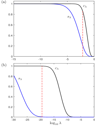
Figure 1: Size $s_{\lambda}$ and credibility $c_{\lambda}$ of the BLRs $\mathcal{R}_{\lambda}$, plotted against $\log_{10}\lambda$, for (a) the qubit amplitude-damping channel, and (b) the qutrit amplitude-damping channel. The red vertical dashed lines mark the respective critical $\lambda$ values, ${\lambda_{\text{crit}}=0.0073}$ for (a), and ${\lambda_{\text{crit}}=3.5598\times 10^{-20}}$ for (b). These identify the plausible regions.

As a first example, we look at single-qubit channels. The input states $\rho^{(i)}$ for process tomography are taken to be the tetrahedron states,

$$\rho^{(i)}=\tfrac{1}{2}(\mathbbm{1}+\bm{a}_{i}\cdot\bm{\sigma}),\quad i=1,2,3,\textrm{ and }4,$$ (41)

where $\bm{a}_{i}=3^{-1/2}\bm{v}_{i}$ with the vertex vectors of Eq. (III.2). For every $i$, we use the same POVM, the four-outcome tetrahedron measurement, with outcomes

$$\Pi_{k}=\tfrac{1}{4}(\mathbbm{1}+\bm{a}_{k}\cdot\bm{\sigma}),\quad k=1,2,3,\textrm{ and }4.$$ (42)

We simulate data using an amplitude-damping channel described by the Kraus operators

$$E_{0}\equiv{\left(\begin{array}[]{cc}1&0\\ 0&\sqrt{1-\gamma}\end{array}\right)}\quad\textrm{and}\quad E_{1}\equiv{\left(\begin{array}[]{cc}0&\sqrt{\gamma}\\ 0&0\end{array}\right)},$$ (43)

where $\gamma$, the damping parameter, is set to $0.4$. The matrices above refer to the computational basis. For the matrices appear in the rest of this paper, it should be assumed that they refer to the computational basis as well. 24 copies of each input state $\rho^{(i)}$ are measured (simulated), giving a total of 96 counts over the four input states. The simulated data are reported in Table 1.

Table 1: Simulated data for the first example in Sec. IV.1. Each entry $n_{k}^{(i)}$ represents the number of clicks in detector $\Pi_{k}$ when the input state $\rho^{(i)}$ is sent.

$\rho^{(i)}$

$\Pi_{k}$ 1 2 3 4 1 7 5 6 6 2 3 13 4 4 3 2 7 8 7 4 3 7 8 6

For the prior distribution, we choose the conjugate prior,

$$(\textrm{d}p)\,w_{0}(p)\propto(\textrm{d}p)\prod_{i,k=1}^{4}\bigl{(}p_{k}^{(i)}\bigr{)}^{48\bar{p}_{k}^{(i)}},$$ (44)

where ${\bar{p}=\{\bar{p}_{k}^{(i)}\}}$ corresponds to the Born probabilities [see Eq. (10)] for an amplitude-damping channel with $\gamma=0.5$, expressing our prior belief that that is the actual channel. Figure 1(a) shows the size and credibility curves, obtained from MC integration using 500,000 sample points generated from HMC with the channel parameterization of Sec. III. The critical $\lambda$ value for the plausible region is indicated with a red dashed line, with size value $s=0.2102$ and credibility value $c=0.8586$. The true channel is contained in all BLRs with $\lambda<0.0302$ and $c_{\lambda}>0.5511$, and is thus in the plausible region.

Now, qubit channels are simple to characterize and there are many ways of sampling from the space of qubit channels. It is hence useful to see how our sampling algorithm works for examples beyond the qubit situation, for which proper sampling is more challenging. As a second example, we consider an amplitude-damping qutrit (three-dimensional quantum system) channel with the Kraus operators

$$E_{0}\equiv{\left(\begin{array}[]{ccc}1&0&0\\ 0&\sqrt{1-\gamma_{1}}&0\\ 0&0&\sqrt{1-\gamma_{2}}\end{array}\right)},$$ (48)

$$E_{1}\equiv{\left(\begin{array}[]{ccc}0&\sqrt{\gamma_{1}}&0\\ 0&0&0\\ 0&0&0\end{array}\right)},\quad\textrm{and}\quad E_{2}\equiv{\left(\begin{array}[]{ccc}0&0&\sqrt{\gamma_{2}}\\ 0&0&0\\ 0&0&0\end{array}\right)},$$ (55)

for $\gamma_{1}=0.1$ and $\gamma_{2}=0.5$.

The POVM used is one of the symmetric, informationally complete POVM (SIC-POVM) from the one-parameter family of qutrit SIC-POVMs. It can be described by a set of states $\{\ket{\mu_{i}}\}$; when written in the computational basis, they are given explicitly by

$$\begin{pmatrix}\ket{\mu_{1}}\ket{\mu_{2}}\cdots\ket{\mu_{9}}\end{pmatrix}$$

$$\equiv\frac{1}{\sqrt{2}}\begin{pmatrix}1&1&1&0&0&0&\omega&\omega^{*}&1\\ \omega&\omega^{*}&1&1&1&1&0&0&0\\ 0&0&0&\omega&\omega^{*}&1&1&1&1\end{pmatrix},$$ (56)

where $\omega=\textrm{e}^{\textrm{i}{2\pi/3}}$, $\omega^{*}=\omega^{2}$, and $1+\omega+\omega^{2}=0$. The POVM elements are

$$\Pi_{i}=\frac{1}{3}\ket{\mu_{i}}\bra{\mu_{i}},\quad i=1,2,\cdots,9.$$ (57)

The input states are

$$\rho^{(i)}=\ket{\mu_{i}}\bra{\mu_{i}},\quad i=1,2,\cdots,9.$$ (58)

For each of the input states, the number of copies measured is 27, giving a total of 243 counts. The simulated data are reported in Table 2.

Table 2: Simulated data for the second example in Sec. IV.1. Each entry $n_{k}^{(i)}$ represents the number of clicks in detector $\Pi_{k}$ when the input state $\rho^{(i)}$ is sent.

$\rho^{(i)}$

$\Pi_{k}$ 1 2 3 4 5 6 7 8 9 1 8 1 4 1 8 2 1 2 0 2 3 10 3 1 1 2 3 3 1 3 1 1 9 1 2 2 3 5 3 4 8 3 3 4 0 1 4 3 1 5 2 3 3 1 10 2 4 2 0 6 3 4 4 2 0 8 2 2 2 7 3 2 4 2 0 2 9 4 1 8 2 0 4 0 0 2 6 8 5 9 3 3 3 1 5 0 1 3 8

The prior is the primitive prior, i.e., $w_{0}(p)$ is a constant wherever it is nonzero. Figure 1(b) shows the size and credibility curves, obtained from MC integration with 100,000 sample points using HMC and our channel parameterization. As before, the critical $\lambda$ value for the plausible region is indicated by the vertical dashed line. The size and credibility of the plausible region are $s=0.0032$ and $c=0.9990$ respectively. The true channel is contained in all BLRs with $\lambda<1.1560\times 10^{-6}$, and is thus in the plausible region.

IV.2 Marginal likelihood for channel properties

Often, one is only interested in certain properties of a channel, like the fidelity between the output of the channel and its input, rather than a full channel description in the form of its process matrix. If one could directly measure that one quantity of interest, one expects to accomplish the estimation task with significantly fewer uses of the channel than needed for full tomography. However, a direct measurement of the quantity of interest may be difficult to design and implement, while the process tomography measurement is often standard procedure. Even in the latter case, one should still estimate the quantity of interest directly from the tomography data, rather than first estimating the full process matrix and then computing the quantity of interest from that estimate OEI16 .

The key ingredient in making inferences about a property $F$ of a channel from tomographic data $D$ is the marginal likelihood, obtained by integrating the full likelihood $L(D|p)$ over the irrelevant parameters,

$$L(D|F) = \frac{\int(\mathrm{d}p)\,w_{r}(p)\,\delta\bigl{(}F-f(p)\bigr{)}\,L(D|p)}{\int(\mathrm{d}p)\,w_{r}(p)\,\delta\bigl{(}F-f(p)\bigr{)}}$$ (59)

$$\equiv \frac{W_{r,D}(F)}{W_{r,0}(F)},$$

where $W_{r,D(0)}(F)$ is the integral in the numerator(denominator). $f(p)$ is the function that expresses $F$ in terms of the tomographic probabilities $p$, and $w_{r}(p)$ is the prior density on $p$, which induces a prior density on $F$. $\delta\bigl{(}F-f(p)\bigr{)}$ is the Dirac delta function that enforces ${f(p)=F}$. Once we have the marginal likelihood, we can proceed in an analogous way as in Sec. IV.1 to construct the smallest credible interval (SCI) and the plausible interval for $F$, as well as perform other statistical inference tasks based on the marginal likelihood.

We thus need a general procedure for computing the marginal likelihood $L(D|F)$. In Ref. OEI16 , an iterative algorithm was developed for that purpose, requiring the use of random samples according to specified distributions. The reader is referred to Ref. OEI16 for the full description of the iterative algorithm, and to Appendix C for the details relevant for our examples below. Here, we give only a brief account of the basic ideas. The delta functions in the defining equation (59) are difficult to handle in a numerical evaluation of the integrals. Instead, we evaluate the antiderivatives $P_{r,i}(F)$, with respect to $F$, of $W_{r,i}(F)$,

$$P_{r,i}(F)\equiv\int\textrm{d}F\,W_{r,i}(F),\quad i=D,0,$$ (60)

with step functions in place of the delta functions. $P_{r,i}$ can be computed by MC integration. The results are closely fitted with several-parameter functions, and then differentiated to give $W_{r,i}$, and hence the marginal likelihood. This procedure works, in principle; in practice, one runs into numerical accuracy problems. If $w_{r}(p)$ has little weight over some range of $F$, a rather generic situation, $P_{r,0}$ will be very flat there, and its derivative cannot be reliably estimated. To overcome this problem, the crux is to note that, because of the delta functions, the marginal likelihood is invariant under the replacement $w_{r}(p)\rightarrow w_{r}(p)g(f(p))$ for any function $g(F)$ positive over the entire range of $F$. We thus have the freedom to choose the $w_{r}(p)$ used to evaluate $L(D|F)$. This freedom of choice is exploited in the iterative procedure described in Ref. OEI16 , where the estimate of $W_{r,0}$ is successively improved by using an $w_{r}(p)$ modified by the previous (possibly inaccurate) estimate of $W_{r,0}$, until the desired convergence level is reached. Each iterative step requires the ability to sample according to the new $w_{r}(p)$; that is where the HMC algorithm, permitting sampling in accordance to a user-specified distribution, comes in.

Below, we carry out the iterative algorithm and compute the marginal likelihood for two common channel properties, average fidelity $F_{\mathrm{avg}}$ and minimum fidelity $F_{\mathrm{min}}$. We make use of the HMC algorithm made possible by our channel parameterization of Sec. III. Both examples are for qubit channels, and use the same (simulated) tomographic data obtained from tetrahedron input states [see Eq. (41)] and the tetrahedron POVM [see Eq. (42)] for the true channel

$$\mathcal{E}_{\mathrm{Pauli}}(\cdot)\equiv\Bigl{(}1-\sum_{i=x,y,z}p_{i}\Bigr{)}(\cdot)+\sum_{i=x,y,z}p_{i}\sigma_{i}(\cdot)\sigma_{i},$$ (61)

a Pauli channel. Here, the $\sigma_{i}$s are the standard Pauli operators, and $(p_{x},p_{y},p_{z})=(0.05,0.15,0.2)$. The data are generated from 96 uses of the channel. The simulated data are reported in Table 3.

Table 3: Simulated data for the examples in Sec. IV.2. Each entry $n_{k}^{(i)}$ represents the number of clicks in detector $\Pi_{k}$ when the input state $\rho^{(i)}$ is sent.

$\rho^{(i)}$

$\Pi_{k}$ 1 2 3 4 1 9 4 4 7 2 6 6 3 9 3 3 5 10 6 4 8 4 5 7

We regard the Pauli channel as noise acting on our quantum system. We are interested in the fidelity measures, $F_{\mathrm{avg}}$ and $F_{\mathrm{min}}$, quantifying the effect of this noise channel on our system.

IV.2.1 Average Fidelity

The average fidelity $F_{\mathrm{avg}}$ is defined here as the (squared-)fidelity between the input and output of the channel $\mathcal{E}$, averaged over all input pure states according to the Haar measure. We write $F(\psi,\rho)\equiv\langle\psi|\rho|\psi\rangle$ for the square of the fidelity between a pure state $\psi\equiv|\psi\rangle\langle\psi|$ and an arbitrary state $\rho$. Then, the average fidelity for the channel $\mathcal{E}$ is

$$F_{\mathrm{avg}}(\mathcal{E}) \equiv\int\textrm{d}\psi\,\langle\psi|\mathcal{E}(\psi)|\psi\rangle$$

$$=\langle\psi_{0}{\left[\int\textrm{d}U\,U^{\dagger}\mathcal{E}(U\psi_{0}U^{\dagger})U\right]}|\psi_{0}\rangle$$

$$=\frac{1}{d}{\left[1+(d-1)q\right]}.$$ (62)

Here, $\textrm{d}U$ is the Haar measure for the space of unitary operators, and $\psi_{0}$ is some fiducial pure state. In arriving at the last line, we have used a standard result of the twirling operation Emerson05 (namely, the expression in the brackets in the second-to-last line), with $q$ given by

$$q\equiv\frac{1}{d^{2}-1}\sum_{i}\textrm{tr}{\left(\rho_{\mathcal{E}}(O_{i}^{\mathcal{T}}\otimes O_{i})\right)},$$ (63)

where $O_{i}$s are all the traceless elements of an orthonormal (according to the Hilbert-Schmidt inner product) operator basis, containing an element proportional to the identity operator, for the $d$-dimensional $\mathcal{H}$. In the qubit case, $q$ has the explicit formula,

$$q=\frac{1}{3}\textrm{tr}\bigl{(}\rho_{\mathcal{E}}(\sigma_{x}\otimes\sigma_{x}-\sigma_{y}\otimes\sigma_{y}+\sigma_{z}\otimes\sigma_{z})\bigr{)},$$ (64)

where we have chosen the $*$ map such that $|\overline{i}\rangle=|i\rangle$ for $\{|i\rangle\}_{i=0}^{1}$, the $\sigma_{z}$-basis for the qubit (see comment about this choice in the second paragraph of Sec. II).

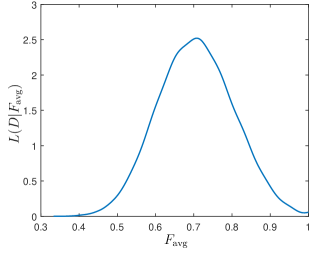
Figure 2: The marginal likelihood $L(D|F_{\mathrm{avg}})$, computed using the iterative procedure of Ref. OEI16 and HMC with our channel parameterization.

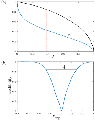
Figure 3: (a) Size (blue) and credibility (green) curves for the bounded likelihood intervals for $F_{\mathrm{avg}}$. The red vertical dashed line marks the critical value of $\lambda$, at ${\lambda_{\text{crit}}=0.3819}$. (b) SCI for $F_{\mathrm{avg}}$. The blue curve indicates the boundaries of the SCIs for different credibility values. The black horizontal line marks the plausible interval and the arrow indicates the true value of ${F_{\mathrm{avg}}=0.7333}$.

We use the iterative procedure of Ref. OEI16 to compute the marginal likelihood $L(D|F_{\mathrm{avg}})$, for $F\equiv F_{\mathrm{avg}}$. The final result is shown in Fig. 2; the intermediate steps of the iterative algorithm are described in Appendix D.1. With the marginal likelihood at hand, as an example of its usefulness, we can construct, as in Sec. IV.1, the SCI for our estimate of $F_{\mathrm{avg}}$. Figure 3(a) gives the size and credibility curves, as well as the critical $\lambda$ value for the plausible region. Figure 3(b) shows the SCI for $F_{\mathrm{avg}}$ for different credibility values. The horizontal black line specifies the plausible interval, which includes the true value of ${F_{\mathrm{avg}}=0.7333}$ (indicated with an arrow).

IV.2.2 Minimum fidelity of unital qubit channels

As a second example, also to illustrate the use of the parameterization of the unital qubit channels of Sec. III.2, we look at the minimum, or worst-case, (squared-)fidelity of a unital channel. The minimum fidelity for a channel $\mathcal{E}$ is the fidelity of the output of $\mathcal{E}$ with its (pure) input, minimized over all input states, i.e.,

$$F_{\mathrm{min}}\equiv\min_{\ket{\psi}}F\bigl{(}\psi,\mathcal{E}(\psi)\bigr{)}.$$ (65)

In the qubit case, $F_{\mathrm{min}}$ can be written explicitly using the Bloch-ball representation as

$$F_{\mathrm{min}}=\min_{\bm{s}:|\bm{s}|=1}\tfrac{1}{2}(1+\bm{s}\cdot\bm{s}_{\mathcal{E}})$$ (66)

where $\bm{s}$ is the Bloch vector of the input state $\psi$, and $\bm{s}_{\mathcal{E}}$ is that of the output $\mathcal{E}(\psi)$. For a unital qubit channel, $\bm{s}_{\mathcal{E}}$ is the image of a linear map on the Bloch vector: $\bm{s}_{\mathcal{E}}=\bm{Ms}$. The minimum fidelity can thus be written simply as

$$F_{\mathrm{min}}=\min_{\bm{s}:|\bm{s}|=1}\tfrac{1}{2}{\left(1+\bm{s}^{T}\bm{Ms}\right)}=\frac{1}{2}(1+\mu_{\text{min}}),$$ (67)

where $\mu_{\text{min}}$ is the smallest eigenvalue of $\frac{1}{2}(\bm{M}+\bm{M}^{\dagger})$. This provides the direct connection between the unital qubit channel and $F_{\mathrm{min}}$, and, in particular, allows us to express $F_{\mathrm{min}}$ in terms of the tomographic probabilities associated with a channel $\mathcal{E}$.

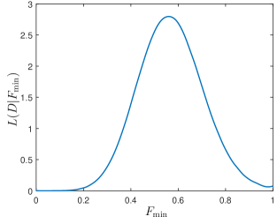
Figure 4: The marginal likelihood $L(D|F_{\mathrm{min}})$, computed using the iterative procedure of Ref. OEI16 and HMC with our channel parameterization.

Here, we assume the promise that the unknown channel is a unital one; the Pauli channel used to simulated the data is indeed unital. In effect, this unitality assumption restricts the relevant space of Choi states dual to the channels, to a strict subset of $\mathscr{S}_{\mathrm{TP}}$, namely, to those that also satisfy Eq. (30). Any channel sampling is thus done only from this subset. Using the parameterization of Sec. III.2, we employ HMC integration to compute the marginal likelihood $L(D|F_{\mathrm{min}})$. The result is given in Fig. 4; the intermediate steps are provided in Appendix D.2. With this marginal likelihood, one can construct the corresponding SCIs and the plausible region, as well as perform other statistical inferences about the unital qubit channel.

IV.3 Model selection

Table 4: Comparison of results based on AIC, BIC, and RBR criteria, with different number of measured copies $N$. Candidate models are nested channel families (see main text). Each row below collects the counts for each family of true channels; each column collects the counts for the model that a criterion selects as the best fit for the data.

		true	# cases where the best-fit model is
		family	Dephasing	Pauli	SUnital	Unital	General
		Dephasing	947	43	10	0	0
		Pauli	583	408	9	0	0
		SUnital	629	319	52	0	0
		Unital	562	405	31	2	0
		General	596	372	30	2	0
		Dephasing	983	17	0	0	0
		Pauli	721	279	0	0	0
		SUnital	795	200	5	0	0
		Unital	741	256	3	0	0
		General	762	235	3	0	0
		Dephasing	712	62	93	56	77
		Pauli	224	271	173	140	192
		SUnital	239	151	315	117	178
		Unital	191	164	215	234	196
$N={20}$	RBR     BIC   AIC	General	166	156	180	164	334
		Dephasing	935	42	21	2	0
		Pauli	305	644	45	6	0
		SUnital	343	429	213	13	2
		Unital	257	534	148	57	4
		General	278	531	115	33	43
		Dephasing	995	4	1	0	0
		Pauli	539	461	0	0	0
		SUnital	646	328	26	0	0
		Unital	601	393	6	0	0
		General	586	404	10	0	0
		Dephasing	823	52	68	22	35
		Pauli	158	404	139	129	170
		SUnital	155	197	376	140	132
		Unital	91	185	222	343	159
$N={50}$	RBR     BIC   AIC	General	75	178	139	176	432
		Dephasing	938	41	18	1	2
		Pauli	173	733	72	16	6
		SUnital	141	368	455	30	6
		Unital	87	409	264	215	25
		General	78	442	147	93	240
		Dephasing	998	2	0	0	0
		Pauli	367	631	2	0	0
		SUnital	427	471	102	0	0
		Unital	357	593	42	8	0
		General	363	609	26	2	0
		Dephasing	905	43	33	11	8
		Pauli	129	578	105	94	94
		SUnital	76	210	506	126	82
		Unital	55	196	223	394	132
$N={100}$	RBR     BIC   AIC	General	34	132	118	190	526

		true	# cases where the best-fit model is
		family	Dephasing	Pauli	SUnital	Unital	General
		Dephasing	933	40	18	7	2
		Pauli	22	866	79	26	7
		SUnital	0	64	818	87	31
		Unital	0	10	85	811	94
		General	0	2	3	47	948
		Dephasing	1000	0	0	0	0
		Pauli	77	923	0	0	0
		SUnital	27	231	742	0	0
		Unital	3	179	250	568	0
		General	2	113	105	112	668
		Dephasing	987	12	1	0	0
		Pauli	36	936	20	8	0
		SUnital	1	92	864	35	8
		Unital	0	18	122	837	23
$N={1\,000}$	RBR     BIC   AIC	General	0	4	7	106	883
		Dephasing	911	49	29	6	5
		Pauli	2	846	99	34	19
		SUnital	0	1	868	94	37
		Unital	0	0	3	889	108
		General	0	0	0	1	999
		Dephasing	1000	0	0	0	0
		Pauli	11	989	0	0	0
		SUnital	0	11	989	0	0
		Unital	0	0	37	963	0
		General	0	0	0	17	983
		Dephasing	999	1	0	0	0
		Pauli	6	993	1	0	0
		SUnital	0	7	985	8	0
		Unital	0	2	60	919	19
$N={10\,000}$	RBR     BIC   AIC	General	0	0	7	86	907
		Dephasing	921	44	27	6	2
		Pauli	1	848	97	37	17
		SUnital	0	0	865	102	33
		Unital	0	0	0	898	102
		General	0	0	0	0	1000
		Dephasing	1000	0	0	0	0
		Pauli	2	998	0	0	0
		SUnital	0	1	999	0	0
		Unital	0	0	1	999	0
		General	0	0	0	1	999
		Dephasing	1000	0	0	0	0
		Pauli	1	999	0	0	0
		SUnital	0	4	994	2	0
		Unital	0	0	68	924	8
$N={100\,000}$	RBR     BIC   AIC	General	0	0	7	80	913

Often, one may not need the full generality of a CPTP channel to describe the dynamics of a quantum system. Instead, a simpler model with fewer parameters may suffice. Simpler models are computationally easier to work with, are likely more easily motivated from a physical standpoint, and may already describe the tomographic data well. One can phrase this problem as one of model selection in statistics, where the best model, among a few candidate models, is chosen, given the available data. Here, we discuss the quantum problem of model selection for channel families. Our sampling algorithm is used for two purposes here: (1) to evaluate a criterion—based on the notion of relative belief—for the “best” model; (2) to assess and compare the performance of different model selection criteria by testing them on many randomly chosen true channels.

Two criteria for model selection commonly used in classical problems are the Akaike Information Criterion (AIC) AIC and the Bayesian Information Criterion (BIC) BIC . The AIC is based on the quantity (which we denote also as “AIC”),

$$\textrm{AIC}=2k-2\log(L_{\text{max}}),$$ (68)

where $k$ is the number of parameters in the model and $L_{\max}$ is the maximum value of the likelihood of the model for the data. The best model is the one with the smallest AIC value. The BIC is defined in a similar manner, but uses the value of $N$, the number of copies measured,

$$\textrm{BIC}=k\log(N)-2\log(L_{\text{max}}).$$ (69)

The best model according to this criterion is again the one with the smallest BIC value.

Another approach to model selection is based on the relative belief ratio (RBR) of Ref. Evans:15 . The RBR of a model $M$ is the ratio of its posterior to prior probabilities,

$$\textrm{RBR}(M|D)=\frac{P(M|D)}{P(M)},$$ (70)

where

$$P(M|D)=\!\int\limits_{M}\!\!(\textrm{d}\rho_{\mathcal{E}})\,\frac{L(D|\rho_{\mathcal{E}})}{L(D)}\quad\textrm{and}\quad P(M)=\!\int\limits_{M}\!\!(\textrm{d}\rho_{\mathcal{E}}).$$ (71)

If the posterior probability for a model $M$ increases after the data, i.e. ${\textrm{RBR}(M|D)>1}$, the data provide evidence in favor of the model; the data provide evidence against the model if ${\textrm{RBR}(M|D)<1}$. It is also useful to have a measure of strength of evidence, since the data might provide evidence in favor of more than one model from our candidate set, and one would like some basis of choosing among those models. The RBR value by itself is not a measure of the strength of evidence (see Ref. Evans:15 for a discussion of various aspects, and also Ref. Evans19 ). We supplement it with the posterior probability

$$P_{M_{0}}\equiv P\bigl{(}[\textrm{RBR}(M|D)=\textrm{RBR}(M_{0}|D)]\,|\,D\bigr{)},$$ (72)

for the model $M_{0}$ in question, and $M$ ranges over the set of candidate models. If ${\textrm{RBR}(M_{0}|D)>1}$ and $P_{M_{0}}$ is large, then there is strong evidence in favor of $M_{0}$. The best model, according to the RBR criterion of relative belief ratio, is the one with the largest posterior probability $P_{M}$, among all candidate models with ${\textrm{RBR}(M|D)>1}$.

As an example, we consider as candidate models five nested qubit channel families: dephasing channels $\subset$ Pauli channels $\subset$ symmetric unital channels $\subset$ unital channels $\subset$ general CPTP channels; see Fig. 5. The smallest set is the 1-parameter family of dephasing channels,

$$\Bigl{\{}\mathcal{D}_{p}(\cdot)\equiv(1-p)(\cdot)+p\sigma_{z}(\cdot)\sigma_{z},p\in[0,1]\Bigr{\}},$$ (73)

and its Choi state is given by

$$\rho_{\mathcal{E}}={\left(\begin{array}[]{cccc}1&0&0&1-2p\\ 0&0&0&0\\ 0&0&0&0\\ 1-2p&0&0&1\end{array}\right)}.$$ (74)

The set of Pauli channels is a 3-parameter family,

$${\left\{\textrm{Pauli}_{\mathbf{p}}(\cdot)\equiv{\Bigl{(}1-\sum_{i}p_{i}\Bigr{)}}(\cdot)+\sum_{i}p_{i}\sigma_{i}(\cdot)\sigma_{i}\right\}},$$ (75)

for $\mathbf{p}\equiv(p_{x},p_{y},p_{z})$, $p_{i}\geq 0$, and $\sum_{i}p_{i}\leq 1$. The Choi state of a Pauli channel is of the form

$$\rho_{\mathcal{E}}={\left(\begin{array}[]{cccc}p_{I}+p_{z}&0&0&p_{I}-p_{z}\\ 0&p_{x}+p_{y}&p_{x}-p_{y}&0\\ 0&p_{x}-p_{y}&p_{x}+p_{y}&0\\ p_{I}-p_{z}&0&0&p_{I}+p_{z}\end{array}\right)},$$ (76)

where $p_{I}=1-p_{x}-p_{y}-p_{z}$. The 6-parameter family of symmetric unital channels refers to the subset of unital qubit channels such that $\bm{R_{1}}=\bm{R_{2}}$ in Eq. (36). We then have the 9-parameter family of unital qubit channels, and lastly, the 12-parameter set of all CPTP qubit channels.

Figure 5: The hierarchy of the five candidate models for the example in Sec. IV.3.

Table 5: A check for bias in the prior. 1000 random channels from each of the channel families are drawn, and data for with different number of measured copies $N$ are simulated for each true channel. The table shows the fraction of instances with evidence against each of the channel families.

true fraction with evidence against family Dephasing Pauli SUnital Unital General Dephasing 0.233 0.812 0.746 0.798 0.810 Pauli 0.724 0.413 0.531 0.401 0.495 SUnital 0.687 0.558 0.398 0.455 0.515 Unital 0.767 0.518 0.508 0.316 0.406 $N={20}$ General 0.779 0.524 0.552 0.384 0.350 Dephasing 0.127 0.802 0.827 0.911 0.916 Pauli 0.786 0.322 0.588 0.511 0.638 SUnital 0.785 0.578 0.326 0.454 0.642 Unital 0.876 0.561 0.503 0.276 0.488 $N={50}$ General 0.892 0.610 0.658 0.448 0.311 Dephasing 0.042 0.844 0.911 0.964 0.978 Pauli 0.826 0.228 0.623 0.672 0.780 SUnital 0.874 0.613 0.249 0.508 0.793 Unital 0.925 0.658 0.573 0.260 0.596 $N={100}$ General 0.948 0.715 0.731 0.576 0.266 Dephasing 0.003 0.966 0.998 1 1 Pauli 0.946 0.028 0.930 0.981 0.999 SUnital 0.992 0.878 0.088 0.868 0.983 Unital 1 0.974 0.821 0.088 0.913 $N={1\,000}$ General 1 0.995 0.983 0.868 0.077 Dephasing 0.001 0.996 1 1 1 Pauli 0.992 0.006 0.996 1 1 SUnital 1 0.992 0.011 0.989 1 Unital 1 0.998 0.930 0.073 0.981 $N={10\,000}$ General 1 1 0.991 0.907 0.092 Dephasing 0 0.999 1 1 1 Pauli 0.999 0.001 1 1 1 SUnital 1 0.996 0.006 0.998 1 Unital 1 1 0.932 0.076 0.992 $N={100\,000}$ General 1 1 0.993 0.920 0.086

A natural prior on the model space is one that puts equal weights on each family. This is easily defined by the sampling procedure: the prior sample is constructed by generating 500,000 sample points with the primitive prior for each family. For the dephasing channel, the sample is generated by sampling $p$ uniformly from $[0,1]$. For the Pauli channel, we obtain the sample by generating $(p_{x},p_{y},p_{z})$ uniformly from the 3-simplex. For the symmetric unital, the unital, and the general channels, we make use of HMC and the parameterizations in Sec. III to generate the sample points. Note that in the numerical procedure that generates the samples for, say, the set of Pauli channels, we will never come across a sample point that is exactly a dephasing channel with ${p_{x}=0=p_{y}}$. Thus, even though the channel families are nested sets, one can consider each family to have prior probability of $\frac{1}{5}$. We use this prior to compute the RBR criterion for simulated data of different sizes. For our choice of prior, $P(M)=\frac{1}{5}$ for all models and $P(M|D)$ is calculated by taking the average of $\frac{L(D|\rho)}{L(D)}$ over the sample points for each model. $P_{M_{0}}$ is computed by summing the posterior probabilities $P(M|D)$ of all the models $M$ with the same RBR as model $M_{0}$. Typically, $P_{M_{0}}=P(M_{0}|D)$.

To assess the performance of the three model-selection criteria, for each family of channels, we randomly (according to the primitive prior, as described above) draw 1000 channels. For each channel, we simulate data—with tetrahedron input states and a tetrahedron measurement [see Eqs. (41) and (42)]—for ${N=20}$, $50$, $100$, $1\,000$, $10\,000$, and $100\,000$ copies measured, and evaluate the AIC, BIC, and RBR criteria for that data. Table 4 shows the conclusions when the three criteria are applied to the simulated data. When the number of measured copies is very small, i.e., $N=20$, the results based on AIC and BIC show a strong bias towards simpler (i.e., fewer-parameters) models. In particular, both criteria rarely identify the right model when the true channel comes from the unital or general families. Results based on RBR, however, show significantly more instances where the correct model is identified for the more complex (i.e., more parameters) models. For a moderate number of measured copies, i.e. ${N=1\,000}$, AIC and RBR give equally good results, whereas BIC shows a slight bias towards the simpler models. When the number of measured copies is very large, i.e., ${N=100\,000}$, results based on BIC are most accurate whereas results based on AIC have a slight bias to the more complex models. RBR also performs well in this regime.

Another aspect that we can check easily with our sampling procedure is the bias in the prior. This is particularly important for model selection based on the RBR criterion, to be sure that the probability of drawing a wrong conclusion is low. For example, for data that are typical for a unital channel, if we were to conclude regularly that there is evidence in favor of the general CPTP model and evidence against the unital model, there is bias in favor of the general CPTP model and bias against the unital model. To check for the bias, we draw 1000 random channels from each of the channel families and simulate data based on these true channels. The number of instances where the simulated data provide evidence against each of the four candidate models are calculated. The results are shown in Table 5. As can be seen from the table, there is no significant bias in the prior when $N\geq 100$, and the bias decreases as the number of measured copies increases.

V Conclusions

In this work, we constructed one exact parameterization for the space of CPTP channels. This parameterization has no superfluous parameters, and requires no imposition of any added constraints. These features make it possible to use the parameterization in a HMC algorithm, for producing high-quality—in terms of low correlations—samples of CPTP channels from a user-specified distribution. We demonstrated the usefulness of our parameterization in sampling applications taken from quantum process tomography. The method applies to general quantum channel sampling problems.

While our parameterization serves the purpose, it is, of course, just one of the many parameterizations that could be used in a HMC algorithm for sampling from the quantum channel space. For example, it is conceivable that a useful parameterization of a channel can be given in terms of the marginals and the copula of the respective Choi state copula . This is unexplored territory.

A useful extension of this work will be to discover also an exact parameterization for the case of CPTP and unital channels. As discussed above, this additional requirement of unitality presents difficulties that can be easily overcome only in the qubit situation. The parameterization for the space of CPTP, unital channels beyond the qubit case, remains an open problem. Note that such a parameterization will give also a possibly useful description of the space of all bipartite mixed quantum states with completely mixed states on both the single-party states; our current parameterization gives the larger space of states where only one of the two single-party states is completely mixed.

Appendix A Hamiltonian Monte Carlo (HMC)

HMC makes use of pseudo-Hamiltonian dynamics in a mock phase space. The parameters of interest are identified as the position variables $\theta$ and fictitious momentum variables $\vartheta$ are introduced. The Hamiltonian is defined as

$$H(\theta,\vartheta)=\frac{1}{2}\sum_{j}\vartheta_{j}^{2}-\log w(\theta),$$ (77)

where $w(\theta)$ is the target distribution. Any reasonable target distribution is permitted and, therefore, one can sample in accordance with any $w(\theta)$.

The HMC algorithm generates a set of sample points which follows the target distribution $w(\theta)$. The HMC algorithm is stated as follows Seah+1:15 :

HMC algorithm

1. Set $j=1$ and choose an arbitrary starting point $\theta^{(1)}$.

2. Generate $\vartheta^{(j)}$ from a multivariate Gaussian distribution with mean zero and unit variance.

3. Solve the Hamiltonian equations of motion

   $$\frac{\mathrm{d}}{\mathrm{d}t}\theta_{i}=\frac{\partial}{\partial\vartheta_{i}}H,\quad\frac{\mathrm{d}}{\mathrm{d}t}\vartheta_{i}=-\frac{\partial}{\partial\theta_{i}}H$$ (78)

   with the initial conditions $(\theta,\vartheta)|_{t=0}=(\theta^{(j)},\vartheta^{(j)})$ to obtain $(\theta^{*},\vartheta^{*})=(\theta,-\vartheta)|_{t=T}$.

4. Calculate the acceptance ratio

   $$a=\min\{1,e^{H(\theta^{(j)},\vartheta^{(j)})-H(\theta^{*},\vartheta^{*})}\}.$$ (79)

5. Draw a random number $b$ uniformly from $[0,1]$. If $b<a$, set $\theta^{(j+1)}=\theta^{*}$; otherwise, set $\theta^{(j+1)}=\theta^{(j)}$.

6. Set $j=j+1$. If $j$ equals the desired number of samples, escape the loop; otherwise, return to step 2.

Note that the $\vartheta$ distribution in step 2 is proportional to the kinetic-energy factor in $\textrm{e}^{-H(\theta,\vartheta)}$; the HMC algorithm enforces a $\theta$ distribution proportional to the potential-energy factor in $\textrm{e}^{-H(\theta,\vartheta)}$, which is $\textrm{e}^{\log w(\theta)}=w(\theta)$, the target distribution. If the differential equations in (78) can be solved exactly, then the acceptance ratio $a=1$. In practice, the differential equations must be discretized. This is done by the leapfrog method. Due to the discretization error, the acceptance ratio will not be 1 generally. The leapfrog method should be implemented such that the acceptance ratio is around the optimal value of $65\%$ Neal11 .

Appendix B Parameterizing qutrit channels

Here, we report an explicit application of the parameterization of Sec. III, for the case of qutrit channels. We start with the permutation matrix $P$ that reshuffles $\varphi_{i}$s into $\psi_{i}$s, with the identically zero entries located below the generically nonzero ones. A $P$ that can accomplish this is one such that

$$P\begin{pmatrix}\begin{smallmatrix}\\ 1\\ 2\\ 3\\ 4\\ 5\\ 6\\ 7\\ 8\\ 9\\ 10\\ 11\\ 12\\ 13\\ 14\\ 15\\ 16\\ 17\\ 18\\ 19\\ 20\\ 21\\ 22\\ 23\\ 24\\ 25\\ 26\\ 27\\ \end{smallmatrix}\end{pmatrix}=\begin{pmatrix}\begin{smallmatrix}\\ 1\\ 10\\ 11\\ 19\\ 20\\ 21\\ 2\\ 3\\ 4\\ 12\\ 13\\ 14\\ 22\\ 23\\ 24\\ 5\\ 6\\ 7\\ 15\\ 16\\ 17\\ 25\\ 26\\ 27\\ 8\\ 9\\ 18\\ \end{smallmatrix}\end{pmatrix}.$$ (80)

After the permutation, we have

$$\psi_{1}=\begin{pmatrix}\psi_{1,1}\\ \vdots\\ \psi_{1,6}\\ 0\\ \vdots\\ 0\end{pmatrix},\quad\psi_{2}=\begin{pmatrix}\psi_{2,1}\\ \vdots\\ \psi_{2,15}\\ 0\\ \vdots\\ 0\end{pmatrix},\quad\psi_{3}=\begin{pmatrix}\psi_{3,1}\\ \vdots\\ \psi_{3,24}\\ 0\\ 0\\ 0\end{pmatrix}.$$ (81)

To parameterize the $\psi_{i}$s such that they are orthonormal, we first parameterize $\psi_{3}$, of unit length,

$$\psi_{3}=\begin{pmatrix}\textrm{e}^{\textrm{i}{\phi_{1}}}\sin\theta_{1}\sin\theta_{2}\cdots\sin\theta_{22}\sin\theta_{23}\\ \textrm{e}^{\textrm{i}{\phi_{2}}}\cos\theta_{1}\sin\theta_{2}\cdots\sin\theta_{22}\sin\theta_{23}\\ \vdots\\ \textrm{e}^{\textrm{i}{\phi_{23}}}\cos\theta_{22}\sin\theta_{23}\\ \textrm{e}^{\textrm{i}{\phi_{24}}}\cos\theta_{23}\\ 0\\ 0\\ 0\end{pmatrix}.$$ (82)

Recalling that $\varphi_{33}$ [see Eq. (12)] is a $d^{2}$-entry real column, and with the $P$ given above, $\psi_{3,4}$, $\psi_{3,5}$, $\psi_{3,6}$, $\psi_{3,13}$, $\psi_{3,14}$, $\psi_{3,15}$, $\psi_{3,22}$, $\psi_{3,23}$, $\psi_{3,24}$ are real. Thus, $\phi_{4}$, $\phi_{5}$, $\phi_{6}$, $\phi_{13}$, $\phi_{14}$, $\phi_{15}$, $\phi_{22}$, $\phi_{23}$, $\phi_{24}$ are set to zero. Then, we define $\{v_{n}\}_{n=1}^{14}$ which lie in the orthogonal subspace of $\psi_{3}$ as follows,

$$v_{1} =\begin{pmatrix}\textrm{e}^{\textrm{i}{\phi_{1}}}\cos\theta_{1}\\ -\textrm{e}^{\textrm{i}{\phi_{2}}}\sin\theta_{1}\\ 0\\ \vdots\\ 0\end{pmatrix},\quad v_{2}=\begin{pmatrix}\textrm{e}^{\textrm{i}{\phi_{1}}}\sin\theta_{1}\cos\theta_{2}\\ \textrm{e}^{\textrm{i}{\phi_{2}}}\cos\theta_{1}\cos\theta_{2}\\ -\textrm{e}^{\textrm{i}{\phi_{3}}}\sin\theta_{2}\\ 0\\ \vdots\\ 0\end{pmatrix},~{}\cdots,$$

$$v_{14} =\begin{pmatrix}\textrm{e}^{\textrm{i}{\phi_{1}}}\sin\theta_{1}\sin\theta_{2}\cdots\sin\theta_{13}\cos\theta_{14}\\ \textrm{e}^{\textrm{i}{\phi_{2}}}\cos\theta_{1}\sin\theta_{2}\cdots\sin\theta_{13}\cos\theta_{14}\\ \vdots\\ \textrm{e}^{\textrm{i}{\phi_{14}}}\cos\theta_{13}\cos\theta_{14}\\ -\textrm{e}^{\textrm{i}{\phi_{15}}}\sin\theta_{14}\\ 0\\ \vdots\\ 0\end{pmatrix}.$$ (83)

To make $\psi_{1}$ and $\psi_{2}$ orthogonal to $\psi_{3}$, we set them to be in the span of $\{v_{n}\}$,

$$\begin{pmatrix}|&|\\ \psi_{1}&\psi_{2}\\ |&|\end{pmatrix} \equiv V\widetilde{\Psi}=\begin{pmatrix}|&|&&|\\ v_{1}&v_{2}&...&v_{14}\\ |&|&&|\end{pmatrix}\begin{pmatrix}|&|\\ \widetilde{\psi}_{1}&\widetilde{\psi}_{2}\\ |&|\end{pmatrix}$$ (84)

The orthonormality of $\psi_{1}$ and $\psi_{2}$ is equivalent to the orthonormality of $\widetilde{\psi}_{1}$ and $\widetilde{\psi}_{2}$. We simply need to repeat the previous procedure. We parameterize $\widetilde{\psi}_{2}$ to be of unit length,

$$\widetilde{\psi}_{2}=\begin{pmatrix}\textrm{e}^{\textrm{i}{\widetilde{\phi}_{1}}}\sin\widetilde{\theta}_{1}\sin\widetilde{\theta}_{2}\cdots\sin\widetilde{\theta}_{12}\sin\widetilde{\theta}_{13}\\ \textrm{e}^{\textrm{i}{\widetilde{\phi}_{2}}}\cos\widetilde{\theta}_{1}\sin\widetilde{\theta}_{2}\cdots\sin\widetilde{\theta}_{12}\sin\widetilde{\theta}_{13}\\ \vdots\\ \textrm{e}^{\textrm{i}{\widetilde{\phi}_{13}}}\cos\widetilde{\theta}_{12}\sin\widetilde{\theta}_{13}\\ \textrm{e}^{\textrm{i}{\widetilde{\phi}_{14}}}\cos\widetilde{\theta}_{13}\\ \end{pmatrix}.$$ (85)

Next, we define $\{u_{n}\}_{n=1}^{4}$, each orthogonal to $\psi_{2}$,

$$u_{1} =\begin{pmatrix}\textrm{e}^{\textrm{i}{\widetilde{\phi}_{1}}}\cos\widetilde{\theta}_{1}\\ -\textrm{e}^{\textrm{i}{\widetilde{\phi}_{2}}}\sin\widetilde{\theta}_{1}\\ 0\\ \vdots\\ 0\end{pmatrix},\qquad u_{2}=\begin{pmatrix}\textrm{e}^{\textrm{i}{\widetilde{\phi}_{1}}}\sin\widetilde{\theta}_{1}\cos\widetilde{\theta}_{2}\\ \textrm{e}^{\textrm{i}{\widetilde{\phi}_{2}}}\cos\widetilde{\theta}_{1}\cos\widetilde{\theta}_{2}\\ -\textrm{e}^{\textrm{i}{\widetilde{\phi}_{3}}}\sin\widetilde{\theta}_{2}\\ 0\\ \vdots\\ 0\end{pmatrix},~{}\ldots,$$

$$u_{4} =\begin{pmatrix}\textrm{e}^{\textrm{i}{\widetilde{\phi}_{1}}}\sin\widetilde{\theta}_{1}\sin\widetilde{\theta}_{2}\sin\widetilde{\theta}_{3}\cos\widetilde{\theta}_{4}\\ \textrm{e}^{\textrm{i}{\widetilde{\phi}_{2}}}\cos\widetilde{\theta}_{1}\sin\widetilde{\theta}_{2}\sin\widetilde{\theta}_{3}\cos\widetilde{\theta}_{4}\\ \textrm{e}^{\textrm{i}{\widetilde{\phi}_{4}}}\cos\widetilde{\theta}_{2}\sin\widetilde{\theta}_{3}\cos\widetilde{\theta}_{4}\\ \textrm{e}^{\textrm{i}{\widetilde{\phi}_{4}}}\cos\widetilde{\theta}_{3}\cos\widetilde{\theta}_{4}\\ -\textrm{e}^{\textrm{i}{\widetilde{\phi}_{5}}}\sin\widetilde{\theta}_{4}\\ 0\\ \vdots\\ 0\end{pmatrix}.$$ (86)

Finally, to have $\widetilde{\psi}_{1}$ normalized and orthogonal to $\widetilde{\psi}_{2}$, we set

$$\widetilde{\psi}_{1} \equiv U\bar{\psi}_{1}=\begin{pmatrix}|&|&&|\\ u_{1}&u_{2}&...&u_{4}\\ |&|&&|\end{pmatrix}\bar{\psi}_{1},$$ (87)

where

$$\bar{\psi}_{1}=\begin{pmatrix}\textrm{e}^{\textrm{i}{\bar{\phi}_{1}}}\sin\bar{\theta}_{1}\sin\bar{\theta}_{2}\sin\bar{\theta}_{3}\\ \textrm{e}^{\textrm{i}{\bar{\phi}_{2}}}\cos\bar{\theta}_{1}\sin\bar{\theta}_{2}\sin\bar{\theta}_{3}\\ \textrm{e}^{\textrm{i}{\bar{\phi}_{3}}}\cos\bar{\theta}_{2}\sin\bar{\theta}_{3}\\ \textrm{e}^{\textrm{i}{\bar{\phi}_{4}}}\cos\bar{\theta}_{3}\end{pmatrix}.$$ (88)

We check that we have the right number of parameters. The parameters used above are $\theta_{1},...,\theta_{23}$, $\phi_{1},...,\phi_{24}$ (nine of these are set identically to zero), $\widetilde{\theta}_{1},...,\widetilde{\theta}_{13}$, $\widetilde{\phi}_{1},...,\widetilde{\phi}_{14}$, $\bar{\theta}_{1},\bar{\theta}_{2},\bar{\theta}_{3}$, and $\bar{\phi}_{1},...,\bar{\phi}_{4}$, giving a total of $72=3^{2}(3^{2}-1)$ parameters, as needed for specifying qutrit channels.

Appendix C Iterative algorithm for estimating the marginal likelihood

To estimate the marginal likelihood reliably, we follow the procedure in Ref. OEI16 . For the following discussion, we assume

$$0\leq f(p)\leq 1,$$ (89)

for the sake of simplicity. First, we note that the integrands in (59) are ill-suited for MC integration due to the presence of the Dirac delta factors. We consider the antiderivatives

$$P_{r,0}(F)=\int(\mathrm{d}p)\,w_{r}(p)\eta\bigl{(}F-f(p)\bigr{)}$$ (90)

and

$$P_{r,D}(F)=\frac{1}{L(D)}\int(\mathrm{d}p)\,w_{r}(p)\eta\bigl{(}F-f(p)\bigr{)}L(D|p).$$ (91)

With a sample of $w_{r}(p)$ and $\frac{\mbox{\footnotesize$w_{r}(p)L(D|p)$}}{\mbox{\footnotesize$L(D)$}}$, we can evaluate the antiderivatives for various values of $F$ and fit them with several-parameters functions. From the fitted functions, we can then calculate the derivatives

$$W_{r,0}(F)=\frac{\partial}{\partial F}P_{r,0}(F)=\int(\mathrm{d}p)\,w_{r}(p)\delta\bigl{(}F-f(p)\bigr{)}$$ (92)

and

$$W_{r,D}(F) =\frac{\partial}{\partial F}P_{r,D}(F)$$

$$=\frac{1}{L(D)}\int(\mathrm{d}p)\,w_{r}(p)\delta\bigl{(}F-f(p)\bigr{)}L(D|p)$$ (93)

and obtain the marginal likelihood by

$$L(D|F)=\frac{W_{r,D}(F)}{W_{r,0}(F)}.$$ (94)

A problem arises when $P_{r,0}(F)$ is very close to a constant over some range of values of $F$. The common situation is that $P_{r,0}(F)$ is very close to zero for a range of values near ${F=0}$ and very close to one for a range of values near ${F=1}$. MC integration is not precise enough to distinguish ${P_{r,0}(F)\gtrsim 0}$ from ${P_{r,0}(F)=0}$ and ${P_{r,0}(F)\lesssim 1}$ from ${P_{r,0}(F)=1}$. As a result, the estimated value of $W_{r,0}(F)$ will be equal to zero over those range of values. We cannot get a reliable estimation of $L(D|F)$ in this situation since $W_{r,0}(F)$ is the denominator in Eq. (94). To overcome this problem, we note that we can do the replacement

$$w_{r}(p)\rightarrow w_{r}(p)g\bigl{(}f(p)\bigr{)}$$ (95)

with an arbitrary function ${g(F)>0}$ without changing the value of $L(D|F)$.

The procedure for obtaining a reliable estimation of $L(D|F)$ is as follows:

1. Sample according to $w_{r}(p)$. Use this sample to calculate $P_{r,0}(F)$. Fit a several-parameters function to $P_{r,0}(F)$ and obtain $W_{r,0}(F)$ by differentiating the fitted function.

2. Sample according to $\widetilde{w}_{r}(p)=\frac{\mbox{\footnotesize$w_{r}(p)$}}{\mbox{\footnotesize$W_{r,0}\bigl{(}f(p)\bigr{)}$}}$. Use this sample to calculate

   $$\widetilde{P}_{r,0}(F)=\int(\mathrm{d}p)\,\widetilde{w}_{r}(p)\eta\bigl{(}F-f(p)\bigr{)}.$$ (96)

   Fit a several-parameters function to $\widetilde{P}_{r,0}(F)$ and obtain $\widetilde{W}_{r,0}(F)$ by differentiating the fitted function.

3. Sample according to $\frac{\mbox{\footnotesize$\widetilde{w}_{r}(p)L(D|p)$}}{\mbox{\footnotesize$L(D)$}}=\frac{\mbox{\footnotesize$w_{r}(p)L(D|p)$}}{\mbox{\footnotesize$W_{r,0}\bigl{(}f(p)\bigr{)}L(D)$}}$. Use this sample to calculate

   $$\qquad\quad\widetilde{P}_{r,D}(F)=\int(\mathrm{d}p)\widetilde{w}_{r}(p)\eta\bigl{(}F-f(p)\bigr{)}L(D|p).$$ (97)

   Fit a several-parameters function to $\widetilde{P}_{r,D}(F)$ and obtain $\widetilde{W}_{r,D}(F)$ by differentiating the fitted function.

4. Obtain the marginal likelihood from

   $$L(D|F)=\frac{\widetilde{W}_{r,D}(F)}{\widetilde{W}_{r,0}(F)}.$$ (98)

The reason that we can have a reliable estimation of $L(D|F)$ using $\widetilde{W}_{r,0}(F)$ obtained in step 2 is as follows. Suppose the exact value of $W_{r,0}(F)$ is known, $\widetilde{W}_{r,0}(F)$ will be equal to $1$ and $\widetilde{P}_{r,0}(F)$ will be equal to $F$. If the exact values of $W_{r,0}(F)$ are not known, but we have a good approximation for $W_{r,0}(F)$ from step 1 and use it for the calculation of $\widetilde{P}_{r,0}(F)$ in step 2, the $\widetilde{P}_{r,0}(F)$ that we obtain will still be quite close to $F$ and $\widetilde{W}_{r,0}(F)$ will be nonzero for all range of $F$ values.

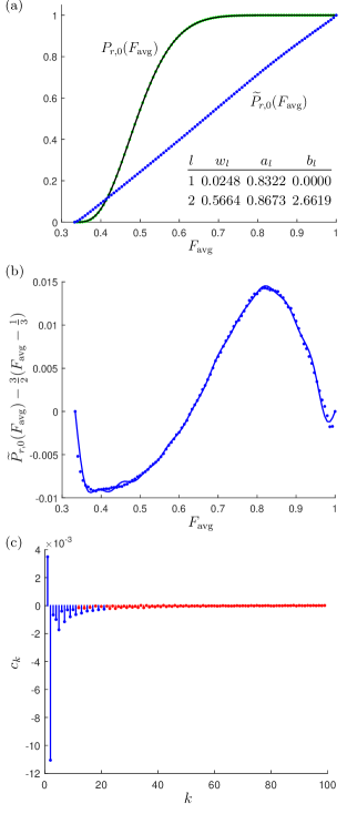
Figure 6: Average gate fidelity. (a) The green dots depict the MC values of $P_{r,0}(F_{\mathrm{avg}})$, and the black curve is fitted to them; the inset table reports the fitting parameters. The values of $\tilde{P}_{r,0}(F_{\mathrm{avg}})$ are traced out by the blue dots. (b) The blue dots show the MC-values of $\tilde{P}_{r,0}(F_{\mathrm{avg}})$ after subtracting the straight line ${\frac{3}{2}(F_{\mathrm{avg}}-\frac{1}{3})}$. The blue curve, a truncated Fourier series, is fitted to the dots. (c) Fourier amplitudes for $\tilde{P}_{r,0}(F_{\mathrm{avg}})$. The high-frequency noise is removed from the fit in (b) by discarding the red amplitudes whose magnitude is less than $2\%$ of that of largest amplitude.

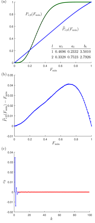
Figure 7: Minimum gate fidelity. (a) The green dots depict the MC values of $P_{r,0}(F_{\mathrm{min}})$, and the black curve is fitted to them; the inset table reports the fitting parameters. The values of $\tilde{P}_{r,0}(F_{\mathrm{min}})$ are traced out by the blue dots. (b) The blue dots show the MC-values of $\tilde{P}_{r,0}(F_{\mathrm{min}})$ after subtracting the straight line $F_{\mathrm{min}}$. The blue curve, a truncated Fourier series, is fitted to the dots. (c) Fourier amplitudes for $\tilde{P}_{r,0}(F_{\mathrm{min}})$. The high-frequency noise is removed from the fit in (b) by discarding the red amplitudes whose magnitude is less than $2\%$ of that of largest amplitude.

In step 1, $P_{r,0}(F)$ can be fitted with a linear combination of regularized incomplete beta functions

$$I_{a,b}(x)=\frac{\int_{0}^{x}t^{a-1}(1-t)^{b-1}\mathrm{d}t}{\int_{0}^{1}t^{a-1}(1-t)^{b-1}\mathrm{d}t},$$ (99)

that is

$$P_{r,0}(F)= w_{1}I_{a_{\text{min}},b_{1}}(F)+w_{2}I_{a_{1},b_{\text{min}}}(F)$$

$$+w_{3}I_{a_{2},b_{2}}(F)+\dots$$

$$+\left(1-\sum_{i=1}^{N-1}w_{i}\right)I_{a_{N-1},b_{N-1}}(F),$$ (100)

with the fitting parameters $a_{1},\dots,a_{N-1},$ $b_{1},\dots,b_{N-1},$ $w_{1},\dots,w_{N-1}$. $a_{\text{min}}$ and $b_{\text{min}}$ are fixed by the power laws satisfy by $P_{r,0}(F)$ near $F=0$ and $F=1$,

$$P_{r,0}(F)\propto F^{a_{\text{min}}}\quad\text{for}\;F\gtrsim 0,$$ (101)

and

$$1-P_{r,0}(F)\propto(1-F)^{b_{\text{min}}}\quad\text{for}\;F\lesssim 1.$$ (102)

In step 2, a truncated Fourier series of the form

$$\widetilde{P}_{r,0}(F)\simeq F +c_{1}\sin(\pi F)+c_{2}\sin(2\pi F)$$

$$+c_{3}\sin(3\pi F)+\cdots$$ (103)

is usually a good fitting function. In step 3, $\widetilde{P}_{r,D}(F)$ can be fitted with a smoothing spline.

Appendix D Intermediate results for the estimation of the marginal likelihood

D.1 Average gate fidelity

The green dots in Fig. 6(a) show the values of $P_{r,0}(F_{\mathrm{avg}})$ obtained by a MC integration with $1\,000\,000$ sample points. The MC integration is not precise enough to distinguish ${P_{r,0}(F_{\mathrm{avg}})\gtrsim 0}$ from ${P_{r,0}(F_{\mathrm{avg}})=0}$ near ${F_{\mathrm{avg}}=\frac{1}{3}}$ and to distinguish ${P_{r,0}(F_{\mathrm{avg}})\lesssim 1}$ from ${P_{r,0}(F_{\mathrm{avg}})=1}$ near ${F_{\mathrm{avg}}=1}$. Therefore, a reliable approximation for $W_{r,0}(F_{\mathrm{avg}})=\frac{\mbox{\footnotesize$\partial$}}{\mbox{\footnotesize$\partial F_{\mathrm{avg}}$}}P_{r,0}(F_{\mathrm{avg}})$ cannot be obtained. To overcome this problem, we follow the procedure stated in Appendix C. First, we fit the green dots with a three-term fitting function of the form of Eq. (C) with ${F=\frac{3}{2}(F_{\mathrm{avg}}-\frac{1}{3})}$, ${a_{\text{min}}=3}$ and ${b_{\text{min}}=\frac{21}{2}}$. The black curve is the fitted curve of $P_{r,0}(F_{\mathrm{avg}})$. The fitting parameters are shown in the inset table. $\widetilde{P}_{r,0}(F_{\mathrm{avg}})$ is obtained from a MC integration with $1\,500\,000$ sample points and shown as the blue dots in Fig. 6(a).

The $\widetilde{P}_{r,0}(F_{\mathrm{avg}})$ is quite close to the straight line ${\frac{3}{2}(F_{\mathrm{avg}}-\frac{1}{3})}$. The $\widetilde{P}_{r,0}(F_{\mathrm{avg}})$ after subtracting the straight line ${\frac{3}{2}(F_{\mathrm{avg}}-\frac{1}{3})}$ is shown as the blue dots in Fig. 6(b). The blue curve shows the fitting curve, a truncated Fourier series whose Fourier amplitudes are reported in Fig. 6(c).

$\widetilde{P}_{r,D}(F_{\mathrm{avg}})$ is evaluated by a MC integration with $1\,500\,000$ sample points and it can be fitted with a smoothing spline. The marginal likelihood shown in Fig. 2 is obtained from the ratio of $\widetilde{W}_{r,D}(F_{\mathrm{avg}})$ and $\widetilde{W}_{r,0}(F_{\mathrm{avg}})$.

D.2 Worst-case fidelity of a unital qubit channel

The green dots in Fig. 7(a) show the values of $P_{r,0}(F_{\mathrm{min}})$ from a MC integration with $1\,000\,000$ sample points. The MC integration is not precise enough to distinguish ${P_{r,0}(F_{\mathrm{min}})\gtrsim 0}$ from ${P_{r,0}(F_{\mathrm{min}})=0}$ near ${F_{\mathrm{min}}=0}$ and to distinguish ${P_{r,0}(F_{\mathrm{min}})\lesssim 1}$ from ${P_{r,0}(F_{\mathrm{min}})=1}$ near ${F_{\mathrm{min}}=1}$. Therefore, a reliable approximation for ${W_{r,0}(F_{\mathrm{min}})=\frac{\mbox{\footnotesize$\partial$}}{\mbox{\footnotesize$\partial F_{\mathrm{min}}$}}P_{r,0}(F_{\mathrm{min}})}$ cannot be obtained. To overcome this problem, we follow the procedure stated in Appendix C. First, we fit the green dots with a three-term fitting function of the form in Eq. (C) with ${F=F_{\mathrm{min}}}$, ${a_{\text{min}}=4}$, and ${b_{\text{min}}=\frac{15}{2}}$. The black curve is fitted to the numerical values for $P_{r,0}(F_{\mathrm{min}})$. The fitting parameters are shown in the inset table. $\widetilde{P}_{r,0}(F_{\mathrm{min}})$ is obtained by a MC integration with $1\,500\,000$ sample points and shown as the blue dots in Fig. 7(a).

The values of $\widetilde{P}_{r,0}(F_{\mathrm{min}})$ are quite close to the straight line $F_{\mathrm{min}}$. The corresponding values after subtracting this straight line make up the blue dots in Fig. 7(b). The blue fitting curve is a truncated Fourier series with the Fourier amplitudes of Fig. 7(c).

$\widetilde{P}_{r,D}(F_{\mathrm{min}})$ is evaluated by a MC integration with $1\,500\,000$ sample points and it can be fitted with a smoothing spline. The marginal likelihood shown in Fig. 4 is the ratio of $\widetilde{W}_{r,D}(F_{\mathrm{min}})$ and $\widetilde{W}_{r,0}(F_{\mathrm{min}})$.

References

- (1) J. Shang, Y.-L. Seah, H. K. Ng, D. J. Nott, and B.-G. Englert, Monte Carlo sampling from the quantum state space. I, New J. Phys. 17, 043017 (2015).
- (2) Y.-L. Seah, J. Shang, H. K. Ng, D. J. Nott, and B.-G. Englert, Monte Carlo sampling from the quantum state space. II, New J. Phys. 17, 043018 (2015).
- (3) K. Życzkowski, P. Horodecki, A. Sanpera, and M. Lewenstein, Volume of the set of separable states, Phys. Rev. A 58, 883 (1998).
- (4) K. Życzkowski, Volume of the set of separable states. II, Phys. Rev. A 60, 3496 (1999).
- (5) K. Życzkowski, and H.-J. Sommers, Induced measures in the space of mixed quantum states, J. Phys. A: Math. Gen. 34, 7111 (2001).
- (6) R. Blume-Kohout, Optimal, reliable estimation of quantum states, New J. Phys. 12, 043034 (2010).
- (7) F. Huszár and N. M. T. Houlsby, Adaptive Bayesian quantum tomography, Phys. Rev. A 85, 052120 (2012).
- (8) C. Oh, Y. S. Teo, and H. Jeong, Efficient Bayesian credible-region certification for quantum-state tomography, Phys. Rev. A 100, 012345 (2019).
- (9) M.-D. Choi, Completely positive linear maps on complex matrices, Linear Algebra Appl. 10, 285 (1975).
- (10) A. Jamiołkowski, Linear transformations which preserve trace and positive semidefiniteness of operators, Rep. Math. Phys. 3, 275 (1972).
- (11) L. P. Thinh, P. Faist, J. Helsen, D. Elkouss, and S. Wehner, Practical and reliable error bars for quantum process tomography, Phys. Rev. A 99, 052311 (2019).
- (12) I. Bengtsson and K. Życzkowski, Geometry of Quantum States: An Introduction to Quantum Entanglement (Cambridge University Press, Cambridge, 2006 and 2017).
- (13) W. Bruzda, V. Cappellini, H.-J. Sommers, and K. Życzkowski, Random Quantum Operations, Phys. Lett. A 373, 320 (2009).
- (14) W. Bruzda, M. Smaczyński, V. Cappellini, H.-J. Sommers, and K. Życzkowski, Universality of spectra for interacting quantum chaotic systems, Phys. Rev. E 81, 066209 (2010).
- (15) R. M. Neal, Bayesian Learning for Neural Networks, Lecture Notes in Statistics, Vol. 118. (Springer, Heidelberg, 1996).
- (16) A. Hajian, Efficient cosmological parameter estimation with Hamiltonian Monte Carlo technique, Phys. Rev. D 75, 083525 (2007).
- (17) E. K. Porter and J. Carré, A Hamiltonian Monte Carlo method for Bayesian Inference of Supermassive Black Hole Binaries, Class. Quant. Grav. 31, 145004 (2014).
- (18) R. M. Neal, MCMC using Hamiltonian dynamics, in: Handbook of Markov Chain Monte Carlo, edited by S. Brooks, A. Gelman, G. Jones and X.-L. Meng (Chapman and Hall, Boca Raton, 2011), Chapter 5.
- (19) S. Duane, A. D. Kennedy, B. J. Pendleton, and D. Roweth, Hybrid Monte Carlo, Phys. Lett. B 195, 216 (1987).
- (20) T. Durt, B.-G. Englert, I. Bengtsson, and K. Życzkowski, On Mutually Unbiased Bases, Int. J. Quant. Phys. 8, 535 (2010).
- (21) Z. Hradil, J. Řeháček, J. Fiurášek, and M. Ježek, Maximum-Likelihood Methods in Quantum Mechanics, in: Quantum State Estimation, edited by M. Paris and J. Řeháček, Lecture Notes in Physics, Vol. 649 (Springer, Heidelberg, 2004), Chapter 3.
- (22) An alternative, equally straightforward, parameterization exploits that the two-qubit Choi states for unital channels have real matrices in the “magic basis” Hill-Wootters97 , composed of the singlet state and the three triplet states , , and .
- (23) J. Shang, H. K. Ng, A. Sehrawat, X. Li, and B.-G. Englert, Optimal error regions for quantum state estimation, New J. Phys. 15, 123026 (2013).
- (24) M. Evans, Measuring Statistical Evidence Using Relative Belief, Monographs on Statistics and Applied Probability, Vol. 144 (CRC Press, Boca Raton, 2015).
- (25) X. Li, J. Shang, H. K. Ng, and B.-G. Englert, Optimal error intervals for properties of the quantum state, Phys. Rev. A 94, 062112 (2016).
- (26) J. Emerson, R. Alicki, and K. Życzkowski, Scalable Noise Estimation with Random Unitary Operators, J. Opt. B: Quantum Semiclass. Opt. 7, S347 (2005).
- (27) H. Akaike, Information theory and an extension of the maximum likelihood principle, in: Proceedings of the 2nd International Symposium on Information Theory, edited by B. N. Petrov and F. Cáski (Akadémiai Kiadó, Budapest, 1973).
- (28) G. Schwarz, Estimating the dimension of a model, Ann. Stat. 6, 461 (1978).
- (29) M. Evans and Y. Guo, Measuring and Controlling Bias for Some Bayesian Inferences and the Relation to Frequentist Criteria, eprint arXiv:1903.01696 [math.ST] (2019).
- (30) S. Hill and W. K. Wootters, Entanglement of a Pair of Quantum Bits, Phys. Rev. Lett. 78, 5022 (1997).
- (31) A. Lovas and A. Andai, On the notion of quantum copulas, eprint arXiv:1902.08460 [math-ph] (2019).